Time-dependent calculations of transfer ionization by
fast proton-helium collision in one-dimensional kinematics

Abstract

We analyze a transfer ionization (TI) reaction in the fast proton-helium collision $\rm H^{+}+He\to H^{0}+He^{2+}+e^{-}$ by solving a time-dependent Schrödinger equation (TDSE) under the classical projectile motion approximation in one-dimensional kinematics. In addition, we construct various time independent analogues of our model using lowest order perturbation theory in the form of the Born series. By comparing various aspects of the TDSE and the Born series calculations, we conclude that the recent discrepancies of experimental and theoretical data may be attributed to deficiency of the Born models used by other authors. We demonstrate that the correct Born series for TI should include the momentum space overlap between the double ionization amplitude and the wave function of the transferred electron.

I Introduction

The transfer ionization (TI) reaction in a fast proton-helium collision $\rm H^{+}+He\to H^{0}+He^{2+}+e^{-}$ has been studied thoroughly, both experimentally and theoretically, for a long time. Experimental observation of the fully differential momentum distribution of the ejected electron Mergel et al (2001) revealed the potential of this reaction to examine radial and angular correlations in the helium atom ground state. This potential was further explored in Schmidt-Böcking et al (2003); Schmidt-Böking et al (2003). Later on, the experimental set up was improved to detect the complete three-particle coincidence $\rm H-He^{2+}-e^{-}$ and to map three-dimensional ejected electron momentum distributions Schöffler et al (2013a, b); Godunov et al (2005). On the theoretical side, various calculations were performed employing the lowest order perturbation theory in the form of the Born series. The initial first Born results Godunov et al (2004, 2005) confirmed that the fully differential cross sections for TI were indeed a sensitive probe of the ground state correlation in the helium atom ground state. By employing ground state wave functions of various level of sophistication, better or worse agreement with the experiment could be achieved. A more detailed comparison with experimental data, in the form of the fully differential cross sections, was not possible at the time. Indeed, in the earlier experiments Mergel et al (2001); Schmidt-Böcking et al (2003), the momentum distribution of the ionized electron was derived from the momentum and energy conservation with other collision partners, but not directly measured as in the latest experiments Schöffler et al (2013a, b). Nevertheless, the authors of Ref. Godunov et al (2004) continued their quest and included the second Born corrections into their model in the form of the closure term Godunov et al (2008). Improvement to the first Born results was marginal in terms of their agreement with the experimental data.

A similar first Born model of another group of authors Houamer et al (2010) was used to interpret three-dimensional electron-momentum distributions in a series of joint experimental and theoretical works Schöffler et al (2013a, b). Similarly to the initial studies by Godunov et al Godunov et al (2004, 2005, 2008), a strong sensitivity of the calculated results was demonstrated to the quality of the helium atom ground state wave function. However, agreement with the experimental data was qualitative at best. It was hoped that extension of the theoretical model to the second Born treatment would have improved this agreement. However, such an extension reported earlier Godunov et al (2008) was not very efficient. General utility of the second Born corrections is discussed in Kheifets et al (1999).

In their perturbative treatment, both groups of authors identified three terms in the first Born amplitude of the TI reaction. These terms can be associated with various terms of the interaction potential $V_{p1}+V_{p2}+V_{Np}$ when this amplitude is expressed in its prior form. This potential describes the interaction of the projectile proton with the two target electrons and the nucleus.

The first term, associated with $V_{p1}$ and denoted by $A_{1}$ in Houamer et al (2010); Schöffler et al (2013a, b) or termed “transfer first” in Godunov et al (2004, 2005, 2008), is shown to be identical to the Oppenheimer, Brinkmann, and Kramers (OBK) amplitude and describes the collision between the target electron labeled 1 and the proton followed by the capture of this electron by the projectile. The second electron, labeled 2, is released due to rearrangement in the helium atom, known as the shake-off (SO) process. In principle, in the $\rm e-H^{+}$ interaction can be factored out from the OBK term $A_{1}$ Schöffler et al (2013a). The remaining SO amplitude provides a simplified theoretical treatment of TI that was applied in Schmidt-Böcking et al (2003); Schmidt-Böking et al (2003). The second term, associated with $V_{p2}$ and denoted by $A_{2}$ or termed as “ionization first”, describes the process in which the proton knocks off a target electron 1 into the continuum, followed by capturing the remaining electron 2 from the helium atom. The third term, associated with $V_{pN}$ and denoted by $A_{3}$ represents an initial interaction between the projectile and the helium nucleus followed by the electron capture. Similarly to $A_{1}$, the second electron is also released due to the sudden rearrangement in the helium ion.

Unlike the other authors, Voitkiv et al Voitkiv et al (2008); Voitkiv (2008); Voitkiv and Ma (2012) expressed the first Born amplitude in the post form which contained a different interaction potential $V_{N1}+V_{p2}+V_{12}+V_{Np}\ .$ They identified an additional electron-electron Auger mechanism of TI associated with the term $V_{12}$. In this mechanism, the electron to be transferred rids itself of the excess energy not via the coupling to the radiation field, as in the radiative capture process, but by interaction with the other electron. In their comment on Voitkiv and Ma (2012), Popov et al (2014) argued that since both the prior and post forms of the first Born amplitude should be identical, the newly discovered electron-electron Auger mechanism was, in fact, contained in the long-known OBK amplitude. In their reply, Voitkiv and Ma (2014) retorted this argument by appealing to the physical intuition and analogy between the TI and other related processes. Other than this appeal, no quantitative arguments were provided.

Outside the first Born treatment lies the process of repeated interaction of the projectile with the target in which both the target electrons are ejected in sequence. This sequential process is known in the electron-impact ionization and double photoionization as the two-step-2 process McGuire (1997). For the purpose of the present study we will call it binary encounter (BE). The signatures of the SO and BE processes in TI can be found in the momentum distribution of the ejected electron. In the BE process, the ejected electron flies predominantly in the forward direction (in the direction of the projectile), due to the momentum transferred from the projectile. In the SO process, the emitted electron flies predominantly backwards because the instantaneous momenta of an electron pair in the helium atom ground state are aligned in the opposite directions. The SO process is contained in the first Born amplitude while the BE process can be only accommodated by further terms in the Born series. At small velocities of the projectile, the BE mechanism dominates whereas at large velocities it is the SO mechanism that becomes dominant.

In the absence of a rigorous theoretical treatment, when the Born series calculations cannot reproduce the experimental data on a quantitative level, an additional insight into the TI reaction can be gained by a non-perturbative approach based on solving the time-dependent Schrödinger equation (TDSE). For a four-body Coulomb problem like TI, the TDSE cannot be solved in its full dimensionality and additional approximations should be made. In the experiments Mergel et al (2001); Schöffler et al (2013a, b), the projectile proton had the velocity $v_{p}\simeq 5$ a.u. and the momentum $p_{p}\simeq 10^{4}$ a.u. This corresponds to the wavelength $\lambda_{p}\sim 10^{-3}$ a.u. which is much less then the atom size. Due to this fact and because of a small relative change of the projectile velocity, the classical projectile motion approximation (CPA) should be sufficiently accurate. The TI reaction in this approximation is described by a six-dimensional TDSE which can be solved, in principle, using modern computational facilities. Nevertheless, for the purpose of the present work, we further simplify the problem and restrict the motion of all the particles to one dimension (1D). We compare results of thus restricted TDSE calculation with various perturbative Born calculations, also reduced to 1D. By analyzing various aspects of the TDSE and the Born series calculations, we conclude that the recent discrepancies of experimental and theoretical data may be explained by deficiency of theoretical approach used by other authors. We demonstrate that the correct Born series for TI should include the momentum space overlap between the ionization amplitude and the wave function of the transferred electron.

II Theoretical model

Within the scope of the CPA, the full-dimensional TDSE takes the form

$$i\frac{\partial\Psi(\mathbf{r}_{1},\mathbf{r}_{2},t)}{\partial t} = \left[\hat{H}_{0}-\frac{1}{|\mathbf{r}_{1}-\mathbf{R}(t)|}-\frac{1}{|\mathbf{r}_{2}-\mathbf{R}(t)|}\right]$$ (1)

$$\hskip 14.22636pt\times\Psi(\mathbf{r}_{1},\mathbf{r}_{2},t)\ ,$$

with the initial condition

$$\Psi(\mathbf{r}_{1},\mathbf{r}_{2},t_{0})=\Phi_{0}(\mathbf{r}_{1},\mathbf{r}_{2})\exp(-iE_{0}t_{0});\quad t_{0}\to-\infty.$$ (2)

Here $\mathbf{R}(t)=(b,0,v_{p}t)$ is a current position of a proton, $b$ is an impact parameter, $\Phi_{0}(\mathbf{r}_{1},\mathbf{r}_{2})$ is the target ground state function, and $\hat{H}_{0}$ is target Hamiltonian, which for the helium atom has the form

$$\hat{H}_{0}=-\frac{1}{2}\nabla_{1}^{2}-\frac{1}{2}\nabla_{2}^{2}-\frac{1}{r_{1}}-\frac{1}{r_{2}}+\frac{1}{|\mathbf{r}_{2}-\mathbf{r}_{1}|}.$$ (3)

For a one-dimensional kinematics, Eq. (1) is reduced to two-dimensional TDSE

$$i\frac{\partial\psi(x_{1},x_{2},t)}{\partial t} = \left[\hat{H}_{0}+U_{1}(x_{1}-v_{p}t)+U_{1}(x_{2}-v_{p}t)\right]$$ (4)

$$\hskip 14.22636pt\times\psi(x_{1},x_{2},t)$$

with the initial condition

$$\psi(x_{1},x_{2},t_{0})=\varphi_{0}(x_{1},x_{2})\exp(-iE_{0}t_{0});\quad t_{0}\to-\infty$$ (5)

and the Hamiltonian

$$\hat{H}_{0} = -\frac{1}{2}\frac{\partial^{2}}{\partial x_{1}^{2}}-\frac{1}{2}\frac{\partial^{2}}{\partial x_{2}^{2}}+U_{2}(x_{1})+U_{2}(x_{2})$$ (6)

$$\hskip 85.35826pt+U_{-1}(x_{2}-x_{1}).$$

Here the effective potentials $U_{Z}(x\to\pm\infty)=-Z/|x|$ is taken in the form of a shifted Coulomb potential

$$U_{Z}(x)=-\frac{Z}{|x|+|Z|^{-1}}\ .$$ (7)

With this potential, the He⁺ ion is described by a 1D equation

$$\left[-\frac{1}{2}\frac{\partial^{2}}{\partial x^{2}}+U_{Z}(x)\right]\varphi^{Z}_{n}(x)=\epsilon^{Z}_{n}\varphi^{Z}_{n}(x)$$ (8)

with the ground state energy $\epsilon^{Z}_{0}=-Z^{2}/2$ being equal to the ground state energy of a conventional 3D ion. The ground state wave function

$$\varphi^{Z}_{0}(x)=\sqrt{\frac{2Z}{5}}(1+Z|x|)\exp(-Z|x|)\ ,$$ (9)

when Fourier transformed to the momentum space

$$\varphi^{Z}_{0}(x)=\frac{1}{\sqrt{2\pi}}\int_{-\infty}^{\infty}u^{Z}_{0}(\varkappa)e^{i\varkappa x}d\varkappa\ ,$$ (10)

becomes

$$u^{Z}_{0}(p)=\frac{4}{\sqrt{5\pi Z}}\frac{1}{[1+(p/Z)^{2}]^{2}}\ .$$ (11)

This only differs by a normalization constant from a conventional ground state wave function of a hydrogenic ion in the momentum space

$$u_{100}(p)=\frac{2\sqrt{2}}{\pi Z^{3/2}}\frac{1}{[1+(p/Z)^{2}]^{2}}\ .$$

It is a useful property that allows one to maintain the correct dependence of the TI cross-section on $v_{p}$ which is determined by the momentum space overlap. The Fourier transform of the potential (7)

$$V_{Z}(q) = \int_{-\infty}^{\infty}e^{-iq\xi}U_{Z}(\xi)d\xi,$$

$$= 2Z\left(\sin\left|\frac{q}{Z}\right|\mathrm{Ssi}\left|\frac{q}{Z}\right|+\cos\left|\frac{q}{Z}\right|\mathrm{Ci}\left|\frac{q}{Z}\right|\right),$$

can be expressed via the cosine integral $\mathrm{Ci}\,(x)$ and the shifted sine integral $\mathrm{Ssi}\,(x)$

The wave function of the electron captured by the projectile is

$$\psi_{\text{tr}}(x,t)=\varphi^{1}_{0}(x-v_{p}t)\exp\left[iv_{p}x-i\left(\frac{v_{p}^{2}}{2}+\epsilon^{1}_{0}\right)t\right].$$ (13)

If the second electron is ejected with the momentum $k$, the two-electron wave function of the final state can be written as

$$\psi_{k\text{H}}(x_{1},x_{2},t) = \frac{1}{\sqrt{2}}\times$$

$$\left[\psi_{\text{tr}}(x_{1},t)\varphi_{k}^{2(-)}(x_{2})+\psi_{\text{tr}}(x_{2},t)\varphi_{k}^{2(-)}(x_{1})\right]e^{-i\frac{k^{2}}{2}t}\ ,$$

where $\varphi^{Z(-)}_{k}(x)$ is the continuum state function for the ejected electron with the energy $\epsilon=k^{2}/2$. The amplitude of TI is given by the following expression

$$A(k)=\lim_{t\to\infty}\int_{-\infty}^{\infty}\int_{-\infty}^{\infty}\psi_{k\text{H}}^{*}(x_{1},x_{2},t)\psi(x_{1},x_{2},t)dx_{1}dx_{2}.$$ (15)

In the 1D case, the role of differential cross-section of TI is assumed by the probability density

$$P^{(1)}(k)=\frac{dP}{dk}=|A(k)|^{2}\ .$$ (16)

Using the exchange symmetry of the two-electron wave function $\psi(x_{2},x_{1},t)=\psi(x_{1},x_{2},t)$ , we can split the integration in Eq. (15) in two steps. First, we calculate the wave function of the second electron when the first electron is transferred

$$\chi(x_{2},t)=\sqrt{2}\int_{-\infty}^{\infty}\psi_{\text{tr}}^{*}(x_{1},t)\psi(x_{1},x_{2},t)dx_{2}\ .$$ (17)

Next, we calculate the amplitude of ejection of the second electron

$$A(k)=\lim_{t\to\infty}\int\limits_{-\infty}^{\infty}\varphi^{2(-)*}_{k}(x)\exp\left(i\frac{k^{2}}{2}t\right)\chi(x,t)dx\ .$$ (18)

In the second step, for extraction of the ionization amplitudes from $\chi(x_{2},t)$, we used the e-surff method Serov et al (2013). Eq. (4) was solved numerically using the simplest 3-point finite difference scheme for evaluation of the space derivatives, and the split-step method for the time evolution. The target ground state function $\varphi_{0}(x_{1},x_{2})$ was calculated using the evolution in the imaginary time providing the ground state energy $E_{0}=-3.35$ a.u.

To compare the role of the SO and BE processes, we also performed calculations for the case of zero inter-electron potential. In such a case, the SO is absent and only the BE contributes to TI. For that reason we named this approximation BECPA. In this approximation, Eq. (4) can be split in two identical equations

$$i\frac{\partial\psi(x,t)}{\partial t}=\left[\hat{h}_{0}+U_{1}(x-v_{p}t)\right]\psi(x,t)$$ (19)

with

$$\hat{h}_{0}=-\frac{1}{2}\frac{\partial^{2}}{\partial x^{2}}+U_{2}(x)$$ (20)

and the initial condition

$$\psi(x,t_{0})=\varphi^{2}_{0}(x)e^{-i\epsilon^{2}_{0}t_{0}};\quad t_{0}\to-\infty.$$ (21)

The wave function of a non-transferred electron in this approximation is

$$\chi(x,t)=\sqrt{2}C_{\text{tr}}[\psi(x,t)-C_{\text{tr}}\psi_{\text{tr}}(x,t)]\ ,$$ (22)

where the transfer amplitude is

$$C_{\text{tr}}=\lim\limits_{t\to\infty}\int_{-\infty}^{\infty}\psi_{\text{tr}}^{*}(x,t)\psi(x,t)dx.$$ (23)

III Results and discussion

The probability density $P^{(1)}(k)$ (16) as a function of the ejected electron momentum is shown in Fig. 1 for the three selected proton velocities $v_{p}=3$ a.u. (top), 5 a.u. (middle) and 10 a.u. (bottom). Results of the full CPA and BECPA are shown with the black solid line and red dashed line, respectively. The probability density displays two peaks near $k=0$ and $k=2v_{p}$. The origin of the second peak is clear if we consider TI in the rest frame of the projectile. In this frame, the initial electron wave packet is scattered on the proton and part of it is reflected back. This reflected part of the wavepacket has velocity $2v_{p}$ in the laboratory frame. The peak near $k=0$ is splitted by the kinematic node at $k=0$. This node is a characteristic feature for 1D systems with attractive potentials.

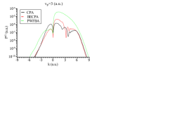
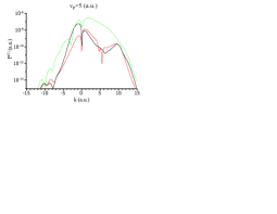
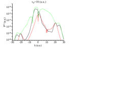
Figure 1: (Color online) The TI probability density $P^{(1)}(k)$ as a function of the ejected electron momentum for the proton velocities $v_{p}=3$ a.u. (top), 5 a.u. (middle) and 10 a.u. (bottom). Various calculations are displayed with the following line styles: the full CPA (black solid line), the BECPA (red dashed line) and the PWFBA (green dotted line).

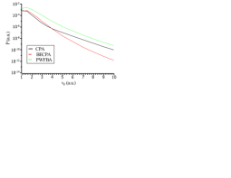
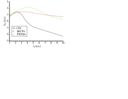
Figure 2: (Color online) The TI probability $P$ (top) and the mean momentum of ejected electrons $\langle k\rangle$ (bottom) as functions of the projectile velocity $v_{p}$. Various calculations are shown as CPA (black solid line), BECPA (red dashed line), PWFBA (green dotted line).

The most essential feature of the experimental differential cross-sections reported by Schöffler et al Schöffler et al (2013a, b) is the shift of the maximum of the ejected electron momentum distribution in the direction opposite to the projectile motion. In the meantime, the 1st Born cross-sections, reported in the same works, display the main peak which is largely centered around the zero momentum.

It is clearly seen in Fig. 1 that the CPA results demonstrate the same backward shift of the main peak, except for the case of the smallest $v_{p}=3$ a.u. The BECPA results demonstrate the forward shift for all $v_{p}$. It is easy to explain this behavior by the following qualitative arguments. In the BE process, both the electrons are pushed by projectile, and ionization occurs irrespective of transfer. Since the momentum transferred from the projectile is directed forward, main peak in the ionization probability is also shifted forward. In the SO process, the second electron is preferably ejected in the direction opposite to the first electron motion which is captured by projectile. The resulting preferable ejection direction depends on the relative weighting of the BE and SO process. Since the SO appears in the first term of the Born series over the projectile-target interaction, and the BE can only be accommodated by the second and further terms, the SO is dominant at larger $v_{p}$, where the ejected electron should be emitted preferentially in the direction opposite to the projectile motion.

To compare the relative contributions of the BE and SO processes and the direction of the preferred emission of the ejected electron depending on $v_{p}$, we calculated the total probability of TI and the mean momentum of the ejected electron

$$P = \int_{-\infty}^{\infty}P^{(1)}(k)dk$$ (24)

$$\langle k\rangle = \frac{1}{P}\int_{-\infty}^{\infty}kP^{(1)}(k)dk.$$ (25)

By comparing the CPA and BECPA results shown in Fig. 2, it is clearly seen the the BE is dominant at $v_{p}<4$ while for larger $v_{p}$ it is the SO that dominates. In about the same momentum range, the mean momentum $\langle k\rangle$ changes its sign. At larger $v_{p}$, the mean momentum becomes large and negative. This indicates that the present CPA results are consistent with the experimental observations. One may suggest that in the first Born approximation (FBA) this preferred backward emission would be even more prominent feature. However, the plane wave first Born approximation (PWFBA) Houamer et al (2010) strongly overestimates forward emission.

This implies that the deviations of the PWFBA calculations from the experiment Schöffler et al (2013a, b) may be attributed to the shortcomings of this specific implementation rather than contribution from the further Born terms.

III.1 Plane-wave first-Born approximation

Let us construct a 1D analogue of the PWFBA. In this approximation, the transitional amplitude takes the form

$$A(k)=\langle p_{H}f|U_{1}(x_{1}-x_{p})+U_{1}(x_{2}-x_{p})-2U_{1}(x_{p})|p_{p}0\rangle\ ,$$ (26)

where the initial state wave function

$$\langle x_{1},x_{2},x_{p}|p_{p}0\rangle = \frac{1}{\sqrt{v_{p}}}e^{ip_{p}x_{p}}\varphi_{0}(x_{1},x_{2})\ .$$ (27)

Following Houamer et al (2010), we express the final state wave function in its asymptotic form

$$\langle x_{1},x_{2},x_{p}|p_{H}f\rangle = \frac{1}{\sqrt{2v_{H}}}e^{ip_{f}x_{p}}\times$$

$$\left[e^{iv_{H}x_{1}}\varphi^{1}_{0}(x_{1}-x_{p})\varphi_{k}^{2(-)}(x_{2})+e^{iv_{H}x_{2}}\varphi^{1}_{0}(x_{2}-x_{p})\varphi_{k}^{2(-)}(x_{1})\right]\ .$$

Here $v_{H}$ is the velocity of the neutral hydrogen atom, $p_{f}=mv_{H}$ is the proton momentum in the final state. The continuum state wave functions are normalized by the 1D factors $v_{p}^{-1/2}$ and $v_{H}^{-1/2}$. The continuum normalization for various dimensionality is addressed in Landau and Lifshitz (1985).

The momentum transfer from the projectile to the target can be expressed as

$$q=p_{p}-p_{f}=m(v_{p}-v_{H})\simeq\frac{1}{v_{p}}\left[\frac{v_{p}^{2}}{2}+\epsilon^{1}_{0}+\frac{k^{2}}{2}-E_{0}\right].$$ (29)

Similarly to Houamer et al (2010), we introduce the momentum difference of the proton projectile and the neutral hydrogen atom.

$$Q=p_{H}-p_{p}=(m+1)v_{H}-mv_{p}=v_{H}-q.$$ (30)

We note that in Houamer et al (2010) this quantity is denoted by $q$ which is reserved in the present work to $q=v_{H}-Q$. Following the cited paper, we split Eq. (26) into the three distinct terms and express them by using the Fourier transform of the functions $\varphi^{1*}_{0}(x-x_{p})$ and $U_{1}(x)$:

$$A_{1}(k)=\sqrt{2}\iiint\limits_{-\infty}^{\hskip 8.53581pt+\infty}dx_{1}dx_{2}dx_{p}e^{iqx_{p}-iv_{H}x_{1}}$$

$$\times \varphi^{1*}_{0}(x_{1}-x_{p})\varphi_{k}^{2(-)*}(x_{2})U_{1}(x_{1}-x_{p})\varphi_{0}(x_{1},x_{2})$$

$$=\int_{-\infty}^{\infty}u^{1*}_{0}(\varkappa)V_{1}(q-\varkappa)I_{k}(v_{H}-q,0)d\varkappa$$

$$A_{2}(k)=\sqrt{2}\iiint\limits_{-\infty}^{\hskip 8.53581pt+\infty}dx_{1}dx_{2}dx_{p}e^{iqx_{p}-iv_{H}x_{1}}$$

$$\times \varphi^{1*}_{0}(x_{1}-x_{p})\varphi_{k}^{2(-)*}(x_{2})U_{1}(x_{2}-x_{p})\varphi_{0}(x_{1},x_{2})$$

$$=\int_{-\infty}^{\infty}u^{1*}_{0}(\varkappa)V_{1}(q-\varkappa)I_{k}(v_{H}-\varkappa,-q+\varkappa)d\varkappa$$

$$A_{3}(k)=-2\sqrt{2}\iiint\limits_{-\infty}^{\hskip 8.53581pt+\infty}dx_{1}dx_{2}dx_{p}e^{iqx_{p}-iv_{H}x_{1}}$$

$$\times \varphi^{1*}_{0}(x_{1}-x_{p})\varphi_{k}^{2(-)*}(x_{2})U_{1}(x_{p})\varphi_{0}(x_{1},x_{2})$$

$$=-2\int_{-\infty}^{\infty}u^{1*}_{0}(\varkappa)V_{1}(q-\varkappa)I_{k}(v_{H}-\varkappa,0)d\varkappa$$

Here we introduced the notation

$$I_{k}(\kappa_{1},\kappa_{2}) = \frac{\sqrt{2}}{(2\pi)^{1/2}}\int_{-\infty}^{\infty}\varphi_{k}^{2(-)*}(x_{2})e^{-i\kappa_{2}x_{2}}$$

$$\times \left[\int_{-\infty}^{\infty}e^{-i\kappa_{1}x_{1}}\varphi_{0}(x_{1},x_{2})dx_{1}\right]dx_{2}.$$

Finally, Eq. (26) takes the form

$$A(k) = \frac{1}{\sqrt{v_{p}v_{H}}}\int_{-\infty}^{\infty}d\varkappa u^{1*}_{0}(\varkappa)V_{1}(v_{H}-Q-\varkappa)$$

$$\left[I_{k}(Q,0)+I_{k}(v_{H}-\varkappa,-v_{H}+Q+\varkappa)-2I_{k}(v_{H}-\varkappa,0)\right]$$

Which, apart from notations, coincides with Eq.(2) of Houamer et al (2010)

In Fig. 1 we display the probability density calculated with the PWFBA. It is clear that this calculation deviates strongly from the non-perturbative CPA calculation. In the PWFBA, the probability density displays a peak at $k>0$ which overshoots strongly the CPA peak, both by the magnitude and the width. As is seen on the bottom panel of Fig. 2, this overestimation leads to the mean momentum $\langle k\rangle>0$ even at large $v_{p}$. Hence, the 1D implementation of the PWFBA displays the same characteristic feature as the original implementation used in Schöffler et al (2013a, b).

In order to elucidate the origin of this behaviour, we express the PWFBA amplitude neglecting the inter-electron interaction. In this case, $\varphi_{0}(x_{1},x_{2})=\varphi^{2}_{0}(x_{1})\varphi^{2}_{0}(x_{2})$ and

$$I_{k}(\kappa_{1},\kappa_{2}) = \frac{\sqrt{2}}{(2\pi)^{1/2}}\int_{-\infty}^{\infty}\varphi_{k}^{2(-)*}(x_{2})e^{-i\kappa_{2}x_{2}}\varphi^{2}_{0}(x_{2})dx_{2}$$

$$\times\int_{-\infty}^{\infty}e^{-i\kappa_{1}x_{1}}\varphi^{2}_{0}(x_{1})dx_{1}=\sqrt{2}u^{2}_{0}(\kappa_{1})I_{k}(\kappa_{2}),$$

where

$$I_{k}(\kappa)=\int_{-\infty}^{\infty}\varphi_{k}^{2(-)*}(x)e^{-i\kappa x}\varphi^{2}_{0}(x)dx\ .$$

Then Eq. (III.1) takes the form

$$A(k) = \frac{\sqrt{2}}{\sqrt{v_{p}v_{H}}}\int_{-\infty}^{\infty}u^{1*}_{0}(\varkappa-v_{H})V_{1}(\varkappa-Q)$$

$$\left[u^{2}_{0}(Q)I_{k}(0)+u^{2}_{0}(\varkappa)I_{k}(Q-\varkappa)-2u^{2}_{0}(\varkappa)I_{k}(0)\right]d\varkappa\ .$$

Since $I_{k}(0)=0$, the only second term survives under the integral sign, i.e.

$$A(k) = A_{2}(k)$$

$$=\frac{\sqrt{2}}{\sqrt{v_{p}v_{H}}}\int_{-\infty}^{\infty}u^{1*}_{0}(\varkappa-v_{H})V_{1}(\varkappa-Q)I_{k}(Q-\varkappa)u^{2}_{0}(\varkappa)d\varkappa.$$

The authors of Ref. Houamer et al (2010); Schöffler et al (2013a, b) claim that this term is responsible for the BE process. However, BE should be zero in the FBA. The projectile can only act on one of the target electrons and the second electron makes no transition in the absence of the inter-electron interaction. The reason why the term $A_{2}$ is not zero becomes clear if we write it in its original form as the coordinate integral

$$A_{2}(k) = \sqrt{2}\int_{-\infty}^{\infty}dx_{p}e^{iqx_{p}}\int_{-\infty}^{\infty}dx_{1}e^{-iv_{H}x_{1}}\varphi^{1*}_{0}(x_{1}-x_{p})\varphi^{2}_{0}(x_{1})$$

$$\hskip 14.22636pt\times\int_{-\infty}^{\infty}\varphi_{k}^{2(-)*}(x_{2})U_{1}(x_{2}-x_{p})\varphi^{2}_{0}(x_{2})dx_{2}\ .$$

One can see that the projectile interaction causes ionization (the integral over $x_{2}$) and the transfer takes place due to the non-orthogonality of the initial and final state wave functions

$$\langle\varphi^{2}_{0}(x)|\,e^{iv_{H}x}\varphi^{1}_{0}(x-x_{p})\rangle\neq 0$$

Thus $A_{2}$ is the artifact of the approximation employed in Houamer et al (2010); Schöffler et al (2013a, b).

Note that the term $A_{3}$ appears due to proton-nucleus interaction. In CPA, the proton-nucleus potential only adds an overall time-dependent phase factor to the wave function, and thus is unable to produce change of the electronic state. In the Jackson–Schiff (JS) theory of a related process of simple transfer, an introduction of the proton-nucleus potential compensates a spurious term appearing due to the non-orthogonality of the initial and final states Bates (1952, 1958). For transfer ionization, $A_{3}$ plays an analogous role, but it does not provide the full compensation.

It is possible to eliminate the spurious electron transfer by orthogonalizing the single-particle initial and captured electron states. For this purpose, in Eqs. (III.1), (III.1) and (III.1) one shall replace $\varphi_{0}(x_{1},x_{2})$ by

$$\tilde{\varphi}_{0}(x_{1},x_{2},x_{p})\equiv\varphi_{0}(x_{1},x_{2})$$

$$\hskip 14.22636pt-\langle e^{iv_{H}x_{1}}\varphi^{1}_{0}(x_{1}-x_{p})|\varphi_{0}(x_{1},x_{2})\rangle e^{iv_{H}x_{1}}\varphi^{1}_{0}(x_{1}-x_{p})\ .$$

It is easy to see that $A_{2}\equiv 0$ and $A_{3}\equiv 0$ after this replacement. However, this operation does not assure that $A_{1}$ gives the correct result.

III.2 Other theoretical models of TI in 1D

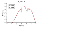
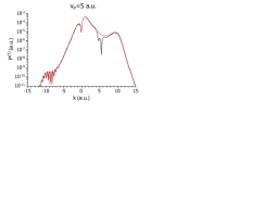
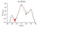
Figure 3: (Color online) Ionization probability density $P^{(1)}(k)$ as a function of the momentum of the ejected electron for the proton velocities $v_{p}=3$ a.u. (top), 5 a.u. (middle) and 10 a.u. (bottom). The following calculations are shown: CPA (black solid line) and FBA (red dashed line).

For further insight, we reduce TI to ionization and transfer of just one electron. The FBA amplitude in this case can be expressed as

$$A_{\text{SI1B}}(k) = \langle p_{f}k|U_{1}(x-x_{p})|p_{p}0\rangle$$

$$=\frac{1}{\sqrt{v_{p}v_{f}}}\langle k|\exp\left(iqx\right)|0\rangle V_{1}(q)=\frac{1}{\sqrt{v_{p}v_{f}}}V_{1}(q)I_{k}(-q)\ ,$$

where the momentum transfer is $q\simeq(k^{2}/2-\epsilon^{2}_{0})/v_{p}$ and the initial and final state wave functions take the form

$$\langle x,x_{p}|p_{p}0\rangle = \frac{1}{\sqrt{v_{p}}}e^{ip_{p}x_{p}}\varphi^{2}_{0}(x);$$ (37)

$$\langle x,x_{p}|p_{f}k\rangle = \frac{1}{\sqrt{v_{f}}}e^{ip_{f}x_{p}}\varphi_{k}^{2(-)}(x).$$ (38)

One can see from Fig. 3 that the FBA and CPA results are quite close except for the electron momenta $k\approx v_{p}$ where the FBA overshoots CPA rather strongly. For these momenta, the electrons are captured by the protons quite efficiently which is not accounted by FBA.

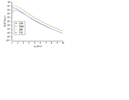
Figure 4: (Color online) Transfer probability as a function of the proton velocity $v_{p}$: CPA (black solid line), OBK (red dashed line), JSB (green dotted line), TSI (blue dot-dashed line).

Now let us consider capture. The OBK amplitude in 1D kinematics has the form

$$C_{\text{OBK}} = \langle p_{f}f|U_{1}(x-x_{p})|p_{p}0\rangle$$

$$= \frac{1}{\sqrt{v_{p}v_{H}}}u^{2}_{0}(v_{H}-q)\int_{-\infty}^{\infty}u^{1*}_{0}(\eta-q)V_{1}(\eta)d\eta\ ,$$

where the momentum transfer $q\simeq(v_{p}^{2}/2+\epsilon^{1}_{0}-\epsilon^{2}_{0})/v_{p}$, and the final state wave function describes the hydrogen atom flying away with the velocity $v_{H}$

$$\langle x,x_{p}|p_{H}f\rangle = \frac{1}{\sqrt{v_{H}}}e^{ip_{f}x_{p}+iv_{H}x}\varphi^{1}_{0}(x-x_{p}).$$ (40)

It is seen from Fig. 4 that the OBK overshoots CPA quite considerably. Now let us check if we can improve the OBK result by a simple orthogonalization of the initial and final state wave functions.

$$\langle x,x_{p}|f_{O}\rangle = e^{iv_{H}x}\varphi^{1}_{0}(x-x_{p})$$

$$- \langle\varphi^{2}_{0}(x)|\,e^{iv_{H}x}\varphi^{1}_{0}(x-x_{p})\rangle\varphi^{2}_{0}(x)$$

It is easy to show that the orthogonalization is equivalent to the OBK formula with the original non-orthogonalized wave functions modified by a perturbation potential

$$C_{\text{JSB}} = \langle p_{f}f|U_{1}(x-x_{p})-\bar{U}_{1}(x_{p})|p_{p}0\rangle\ ,$$ (42)

where the balancing potential

$$\bar{U}_{1}(x_{p}) = \langle 0|U_{1}(x-x_{p})|0\rangle\ .$$ (43)

The balancing potential $\bar{U}_{1}(x_{p})\approx U_{1}(x_{p})$, where $-U_{1}(x_{p})$ can be considered as proton-nucleus potential. Hence, for transfer from the neutral hydrogen, Eq. (42) is close to the JS approximation. Here we consider transfer from the helium ion, and a formal application of the JS approximation for this case gives a perturbation potential $U_{1}(x-x_{p})-U_{2}(x_{p})$. But Bates Bates (1952, 1958) and, lately, Lin et al (1978) have shown that advantage of JS over OBK lie in the fact that the nuclear potential compensates a spurious term from the non-orthogonality of the initial and final state functions. The balancing potential should be used instead of the nuclear potential in a general case Lin et al (1978). For this reasons, the approach given by Eq. (42) can be considered as an improved JS approximation, and we named it as Jackson–Schiff–Bates (JSB) approximation. It is clear from Fig. 4 that the OBK and JSB results differ only at small $v_{p}$, but at large $v_{p}$ both calculations significantly overshoot the CPA.

Now let us tackle the problem from another side. Suppose that, before capture, a real ionization takes place and the ionized electron is captured whose momentum distribution coincides with the momentum space components of the electron bound to the proton. In this case, the TI amplitude will be equal to the overlap integral

$$C_{\text{trSI}} = \int_{-\infty}^{\infty}u^{1*}_{0}(k-v_{H})A_{\text{SI1B}}(k)dk.$$ (44)

We call this approach the transfer via single ionization (TSI) in the first Born approximation. By inspecting Fig. 4 one can conclude that the TSI and CPA results are practically coincident at large $v_{p}$.

In the time-dependent formalism, the TSI is equivalent to solving the following TDSE

$$i\frac{\partial\psi_{1}(x,t)}{\partial t}=\hat{h}_{0}\psi_{1}(x,t)+U_{1}(x-v_{p}t)\varphi^{2}_{0}(x)e^{-i\epsilon^{2}_{0}t}.$$ (45)

and subsequent projection of the solution $\psi_{1}(x,t)$ to the function

$$\tilde{\psi}_{\text{tr}}(x,t)=\int_{-\infty}^{\infty}u^{1}_{0}(k-v_{H})\varphi_{k}^{2(-)}(x)\exp\left(-i\frac{k^{2}}{2}t\right)dk$$ (46)

instead of the function (13). Since the proton potential in Eq. (45) acts solely as a perturbation, the bound state of the proton and electron cannot be described by this equation. The function (46) describes the outgoing wavepacket, but unlike Eq. (13) it is a solution of Eq. (45) at $t\to\infty$. More broadly, the major difference of TSI and OBK/JS is that the Born matrix element is calculated in the former between the eigenfunctions of the same Hamiltonian $\hat{h}_{0}$, whereas in the latter these functions belong to different Hamiltonians.

III.3 Transfer ionization via double ionization

Similarly TSI for simple transfer, we develop a method to calculate TI via double ionization (TIDI). The double ionization amplitude in the FBA has the form

$$A_{\text{DI1B}}(k_{1},k_{2})=\langle p_{H}k_{1}k_{2}|U_{1}(x_{1}-x_{p})+U_{1}(x_{2}-x_{p})|p_{p}0\rangle$$ (47)

where the initial and final state wave functions

$$\langle x_{1},x_{2},x_{p}|p_{p}0\rangle = \frac{1}{\sqrt{v_{p}}}e^{ip_{p}x_{p}}\varphi_{0}(x_{1},x_{2});$$ (48)

$$\langle x_{1},x_{2},x_{p}|p_{H}k_{1}k_{2}\rangle = \frac{1}{\sqrt{v_{f}}}e^{ip_{f}x_{p}}\varphi_{k_{1}k_{2}}^{(-)}(x_{1},x_{2}).$$ (49)

After integration over $x_{p}$ we obtain

$$A_{\text{DI1B}}(k_{1},k_{2})=\frac{1}{\sqrt{v_{p}v_{f}}}\langle k_{1}k_{2}|\exp\left(iqx_{1}\right)+\exp\left(iqx_{2}\right)|0\rangle V_{1}(q),$$ (50)

where the momentum transfer

$$q=p_{p}-p_{f}\simeq\frac{1}{v_{p}}\left(\frac{k_{1}^{2}}{2}+\frac{k_{2}^{2}}{2}-E_{0}\right).$$ (51)

The TI amplitude is calculated as

$$A_{\text{trDI}}(k) = \sqrt{2}\int_{-\infty}^{\infty}u^{1*}_{0}(k_{1}-v_{H})A_{\text{DI1B}}(k_{1},k)dk_{1}.$$ (52)

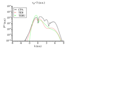
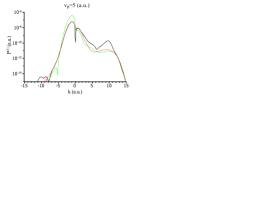
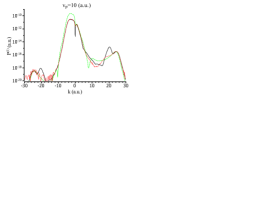
Figure 5: (Color online) TI probability density $P^{(1)}(k)$ as a function of the momentum of the transferred electron for the proton velocities $v_{p}=3$ a.u. (top), 5 a.u. (middle) and 10 a.u. (bottom). Various calculations are shown as CPA (black solid line), TIDI (red dotted line), TIDIU (green dashed line).

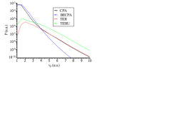
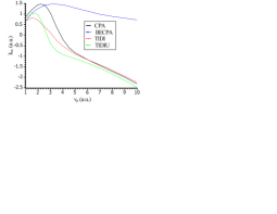
Figure 6: (Color online) The total TI probability $P$ (top) and the mean momentum of ejected electron $\langle k\rangle$ (bottom) as functions of $v_{p}$. Various calculations are shown as CPA (black solid line), TIDI (red dotted line), TIDIU (green dashed line), BECPA (blue dash-dotted line).

From Fig. 5 it is obvious that at large $v_{p}$ and small $k$ the TIDI and CPA results are practically coincident. And from Fig. 6 it is clear that both the total TI probability $P$ and the mean elected electron momentum $\langle k\rangle$, are also very close between the TIDI and CPA in the whole region of dominance of the SO. On the top panel of Fig. 6 the cross-over between the BE and SO mechanisms is seen most graphically: at $v_{p}<4$ the CPA curves is close to that of the BECPA, whereas at $v_{p}>4$ to that of the TIDI.

From Fig. 5 one can observe that for large $k$ the difference between TIDI and CPA is much more prominent. This is explained by a large contribution of the BE process to TI at large $k$ even at large $v_{p}$. By comparing the bottom panels of Fig. 1 and Fig. 5 one can discern some interesting details explaining the origin of a double peak near $k=2v_{p}$. As we mentioned before, this peak appears due to the reflection of the ejected electrons by the proton potential. It is clearly seen on the bottom panel of Fig. 1 the first half of this peak (at lower momenta) is due to the BE process, and from the bottom panel of Fig. 5 it is clear that the second half (at larger momenta) is due to the SO. In the latter case, the sequence events giving rise to TI is the following. First, the impinging proton reflects the electron which flies away with the velocity $k=2v_{p}$, then the second electron, emitted due to the SO, is captured by the proton.

In 3D kinematics, TI can proceed via the nuclear or electron Thomas processes Briggs and Taulbjerg (1979). In these processes, the electron scattered by the proton acquires a velocity $v_{p}$ or $\sqrt{2}v_{p}$ and then, in the secondary scattering from, respectively, the nucleus or the second electron, receives a velocity $\mathbf{v}_{p}$ to be captured by the proton. The Thomas processes are not possible in 1D kinematics because the electron scattered on the proton acquires either zero or $2v_{p}$ velocity in this case.

To pinpoint the role of inter-electron interaction in the final state, we also performed calculations with uncorrelated wave functions of the two-electron continuum orthogonalized to the initial state

$$\tilde{\varphi}_{k_{1}k_{2}}^{(-)}(x_{1},x_{2})=\chi_{k_{1}k_{2}}^{(-)}(x_{1},x_{2})-\langle\chi_{k_{1}k_{2}}^{(-)}|0\rangle\varphi_{0}(x_{1},x_{2}),$$ (53)

where

$$\chi_{k_{1}k_{2}}^{(-)}(x_{1},x_{2})=\frac{1}{\sqrt{2}}\times$$

$$\left[\varphi_{k_{1}}^{2(-)}(x_{1})\varphi_{k_{2}}^{2(-)}(x_{2})+\varphi_{k_{2}}^{2(-)}(x_{1})\varphi_{k_{1}}^{2(-)}(x_{2})\right].$$

This approximation is labeled as TIDIU.

From Fig. 6, it is clear that the TIDIU overestimate significantly the value of $P$. The mean momentum $\langle k\rangle$ is rather close to the exact solution, only slightly overestimated in the negative region. It is seen in Fig. 5 that overestimated $P$ is due to a strong growth of the peak at small $k<0$, whereas at small $k>0$ the TIDIU calculation is close to both the TIDI and CPA. Thus, we can conclude that the inter-electron correlation in the final state suppresses partially the backward emission and works out of sync with the correlation in the initial state.

IV Conclusion

We have performed time-dependent calculations of transfer ionization in the fast proton scattering on the helium atom. We solved a time-dependent Schrödinger equation under the classical projectile motion approximation in one-dimensional kinematics. To gain deeper physical insight into specific mechanisms of the TI reaction, we also performed various perturbative 1D calculations which mimicked realistic first Born calculations performed by other authors. We identified a strong effect of the non-orthogonality of the initial and final states which may lead to some spurious unphysical terms. This term may be responsible for poor performance of the FBA employed by other authors.

Among various approximate perturbative TI schemes, the most accurate calculation is obtained by overlapping the double ionization amplitude with the momentum profile of the final state wave function. This indicates that the most probable scenario of TI involves double ionization and subsequent capture of those of the ionized electrons which falls into the attractive potential well of the proton by matching its velocity.

Because both Godunov et al Godunov et al (2004, 2005, 2008), and Popov et al Houamer et al (2010); Schöffler et al (2013a, b) employ a very similar formalism based on the Jackson–Schiff approximation, our remarks on possible flaws of the FBA concern both groups of authors. More broad is the question of using non-orthogonal initial and final states belonging to different Hamiltonians in perturbative calculations. This question goes beyond the scope of the present work. The same question was a matter of discussion in theory of simple transfer much earlier Lin (1978); Lin et al (1978); Bates (1952, 1958).

In future, we intend to extend our 1D model to full dimensionality under the same classical projectile motion approximation.

We acknowledge Markus Schöffler and Reinhard Dörner for critical reading of the manuscript and Yuri Popov for useful and stimulating discussions. V.V.S. acknowledges support from the Russian Foundation for Basic Research (Grant No. 14-01-00420-a).

References

- Mergel et al (2001) V. Mergel, R. Dörner, K. Khayyat, M. Achler, T. Weber, O. Jagutzki, H. J. Lüdde, C. L. Cocke, and H. Schmidt-Böcking, Strong correlations in the He ground state momentum wave function observed in the fully differential momentum distributions for the transfer ionization process, Phys. Rev. Lett. 86, 2257 (2001).
- Schmidt-Böcking et al (2003) H. Schmidt-Böcking, V. Mergel, R. Dörner, C. L. Cocke, O. Jagutzki, L. Schmidt, T. Weber, H. J. Ludde, E. Weigold, Y. V. Popov, et al., Revealing the non- contributions in the momentum wave function of ground state He, Europhys. Lett. 62(4), 477 (2003).
- Schmidt-Böking et al (2003) H. Schmidt-Böking, V. Mergel, R. Dörner, H. J. Lüdde, L. Schmidt, T. Weber, E. Weigold, and A. S. Kheifets, Many-particle quantum dynamics in atomic and molecular fragmentation (Springer, Heidelberg, 2003), chap. Fast -He transfer ionization processes: A window to reveal the non- contributions in the momentum wave function of ground state He, pp. 353–378.
- Schöffler et al (2013a) M. S. Schöffler, O. Chuluunbaatar, Y. V. Popov, S. Houamer, J. Titze, T. Jahnke, L. P. H. Schmidt, O. Jagutzki, A. G. Galstyan, and A. A. Gusev, Transfer ionization and its sensitivity to the ground-state wave function, Phys. Rev. A 87, 032715 (2013a).
- Schöffler et al (2013b) M. S. Schöffler, O. Chuluunbaatar, S. Houamer, A. Galstyan, J. N. Titze, L. P. H. Schmidt, T. Jahnke, H. Schmidt-Böcking, R. Dörner, Y. V. Popov, et al., Two-dimensional electron-momentum distributions for transfer ionization in fast proton-helium collisions, Phys. Rev. A 88, 042710 (2013b).
- Godunov et al (2005) A. L. Godunov, C. T. Whelan, H. R. J. Walters, V. S. Schipakov, M. Schöffler, V. Mergel, R. Dörner, O. Jagutzki, L. P. H. Schmidt, J. Titze, et al., Transfer ionization process with the ejected electron detected in the plane perpendicular to the incident beam direction, Phys. Rev. A 71, 052712 (2005).
- Godunov et al (2004) A. L. Godunov, C. T. Whelan, and H. R. J. Walters, Fully differential cross sections for transfer ionization — a sensitive probe of high level correlation effects in atoms, J. Phys. B 37(10), L201 (2004).
- Godunov et al (2008) A. L. Godunov, C. T. Whelan, and H. R. J. Walters, Effect of angular electron correlation in He: Second-order calculations for transfer ionization, Phys. Rev. A 78, 012714 (2008).
- Houamer et al (2010) S. Houamer, Y. V. Popov, and C. Dal Cappello, Failure of the multiple peaking approximation for fast capture processes at milliradian scattering angles, Phys. Rev. A 81, 032703 (2010).
- Kheifets et al (1999) A. S. Kheifets, I. Bray, and K. Bartschat, Convergent calculations for simultaneous electron-impact ionization-excitation of helium, J. Phys. B 32(15), L433 (1999).
- Voitkiv et al (2008) A. B. Voitkiv, B. Najjari, and J. Ullrich, Mechanism for electron transfer in fast ion-atomic collisions, Phys. Rev. Lett. 101, 223201 (2008).
- Voitkiv (2008) A. B. Voitkiv, Electron-electron interaction and transfer ionization in fast ion-atom collisions, J. Phys. B 41(19), 195201 (2008).
- Voitkiv and Ma (2012) A. B. Voitkiv and X. Ma, Dynamics of transfer ionization in fast ion-atom collisions, Phys. Rev. A 86, 012709 (2012).
- Popov et al (2014) Y. V. Popov, V. L. Shablov, K. A. Kouzakov, and A. G. Galstyan, Comment on “dynamics of transfer ionization in fast ion-atom collisions”, Phys. Rev. A 89, 036701 (2014).
- Voitkiv and Ma (2014) A. B. Voitkiv and X. Ma, Reply to “comment on ‘dynamics of transfer ionization in fast ion-atom collisions’ ”, Phys. Rev. A 89, 036702 (2014).
- McGuire (1997) J. H. McGuire, Electron Correlation Dynamics in Atomic Collisions, Cambridge Monographs on Atomic, Molecular and Chemical Physics (Cambridge University Press, Cambridge, 1997).
- Serov et al (2013) V. V. Serov, V. L. Derbov, T. A. Sergeeva, and S. I. Vinitsky, Hybrid surface-flux method for extraction of the ionization amplitude from the calculated wave function, Phys. Rev. A 88, 043403 (2013).
- Landau and Lifshitz (1985) L. D. Landau and E. M. Lifshitz, Quantum Mechanics (Non-relativistic theory), vol. 3 of Course of theoretical physics (Pergamon press, Oxford, 1985), 3rd ed.
- Bates (1952) D. R. Bates, A. Dalgarno, Electron Capture I: Resonance Capture from Hydrogen Atoms by Fast Protons, Proc. Phys. Soc. A 65, 919 (1952).
- Bates (1958) D. R. Bates, Electron Capture in Fast Collisions, Proc. R. Soc. Lond. A 247, 294 (1958).
- Lin et al (1978) C. D. Lin, S. C. Soong, L. N. Tunnell, Two-state atomic expansion methods for electron capture from multielectron atoms by fast protons, Phys. Rev. A 17, 1646 (1978).
- Briggs and Taulbjerg (1979) J. S. Briggs, K. Taulbjerg, Charge transfer by a double-scattering mechanism involving target electrons, J. Phys. B: Atom. Molec. Phys. 12, 2565 (1979).
- Lin (1978) C. D. Lin, Electron capture for ion-atom collisions at intermediate energies, J. Phys. B 11, L185 (1978).