Ensemble inequivalence in a mean-field XY model with ferromagnetic and nematic couplings

Abstract

We explore ensemble inequivalence in long-range interacting systems by studying an XY model of classical spins with ferromagnetic and nematic coupling. We demonstrate the inequivalence by mapping the microcanonical phase diagram onto the canonical one, and also by doing the inverse mapping. We show that the equilibrium phase diagrams within the two ensembles strongly disagree within the regions of first-order transitions, exhibiting interesting features like temperature jumps. In particular, we discuss the coexistence and forbidden regions of different macroscopic states in both the phase diagrams.

Recent years have seen extensive studies of systems with long-range interactions that have the two-body potential in $d$ dimensions decaying at large separation $r$ as $1/r^{\alpha};0\leq\alpha\leq d$ Campa:2009 ; Bouchet:2010 ; Levin:2014 ; Campa:2014 . Examples span a wide variety, from bacterial population Sopik:2005 , plasmas Nicholson:1992 , dipolar ferroelectrics and ferromagnets Landau:1960 , to two-dimensional geophysical vortices Chavanis:2002 , self-gravitating systems Paddy:1990 , etc. A striking feature of long-range systems distinct from short-range ones is that of non-additivity, whereby thermodynamic quantities scale superlinearly with the system size. Non-additivity manifests in static properties like negative microcanonical specific heat Lynden-Bell:1968 ; Thirring:1970 , inequivalence of statistical ensembles Kiessling:1997 ; Barre:2001 ; Ispolatov:2001 ; Barre:2007 ; Mukamel:2005 ; Venaille:2009 ; Venaille:2011 ; Teles:2014 , and other rich possibilities Bouchet:2005 . As for the dynamics, long-range systems often exhibit broken ergodicity Mukamel:2005 ; Bouchet:2008 , and slow relaxation towards equilibrium Chavanis:2002 ; Mukamel:2005 ; Ruffo:1995 ; Yamaguchi:2004 ; Campa:2007 ; Joyce:2010 .

Here, we demonstrate ensemble inequivalence in a model of long-range systems that has mean-field interaction (i.e., $\alpha=0$) and two coupling modes. This so-called Generalized Hamiltonian Mean-Field (GHMF) model, a long-range version with added kinetic energy of the model of Ref. Lee:1985 , has $N$ interacting particles with angular coordinates $\theta_{i}\in[0,2\pi]$ and momenta $p_{i}$, $i=1,2,\ldots,N$, which are moving on a unit circle Teles:2012 . The GHMF Hamiltonian is

$$H=\sum\limits_{i=1}^{N}\frac{p_{i}^{2}}{2}+\frac{1}{2N}\sum\limits_{i,j=1}^{N}\Big{[}1-\Delta\cos\theta_{ij}-(1-\Delta)\cos 2\theta_{ij}\Big{]},$$ (1)

where $\theta_{ij}\equiv\theta_{i}-\theta_{j}$. Here, $\cos\theta_{ij}$ is an attractive interaction minimized by the particles forming a cluster, so that $\theta_{ij}=0\;(\text{mod }2\pi)$, while $\cos 2\theta_{ij}$ with two minima at $\theta_{ij}=0,\,\pi\;(\text{mod }2\pi)$ promotes a two-cluster state. The parameter $\Delta\in[0,1]$ sets the relative strength of the two coupling modes. The potential energy in (1) is scaled by $N$ to make the energy extensive, following the Kac prescription Kac:1963 , but the system remains non-additive. In terms of the $XY$-spin vectors ${\bf S}_{i}\equiv(\cos~{}\theta_{i},\sin~{}\theta_{i})$, the interactions have the form of a mean-field ferromagnetic interaction $\sim-\Delta{\bf S}_{i}\cdot{\bf S}_{j}$, and a mean-field coupling $\sim-(1-\Delta)({\bf S}_{i}\cdot{\bf S}_{j})^{2}$ promoting nematic ordering. For $XY$ lattice models with this type of ferro-nematic coupling, see Lee:1985 ; Carpenter:1989 ; Park:2008 ; Qi:2013 . The system (1) has Hamilton dynamics: $d\theta_{i}/dt=p_{i},dp_{i}/dt=-\partial H/\partial\theta_{i}$. For $\Delta=1$, when no nematic ordering exists, the GHMF model becomes the Hamiltonian mean-field (HMF) model Ruffo:1995 , a paradigmatic model of long-range systems Campa:2009 .

In this work, we report on striking and strong inequivalence of statistical ensembles for the GHMF model. The system has three equilibrium phases: ferromagnetic, paramagnetic, and nematic, with first and second-order transitions. Let us note that ref. Antoni:2002 studied another model with long-range interactions, which also shows paramagnetic, ferromagnetic and nematic-like phases. For the GHMF model, by comparing the phase diagrams in the canonical and microcanonical ensembles (the latter is derived in Teles:2012 ), we show in the regions of first-order transitions that the phase diagrams differ significantly. We analyze the inequivalence in two ways, by mapping the microcanonical phase diagram onto the canonical one, as is usually done Barre:2001 ; Ispolatov:2001 ; Barre:2007 ; Mukamel:2005 ; Venaille:2009 ; Venaille:2011 ; Teles:2014 , and also by doing the inverse mapping of the canonical onto the microcanonical one; in particular, we discuss the coexistence and forbidden regions of different macroscopic states. This study demonstrates the subtleties and intricacies of the presence of different stability regions of macroscopic states in long-range systems in microcanonical and canonical equilibria. It is worth noting that compared to the the pure para-ferro transition, the phenomenology here due to presence of the additional nematic phase is much more rich. We will show that the region where the three phases meet, within both microcanonical and canonical ensembles, is the one exhibiting ensemble inequivalence.

We now turn to derive our results. Rotational symmetry of the Hamiltonian (1) allows to choose, without loss of generality, the ordering direction in the equilibrium stationary state to be along $x$ (there are no stationary states with a non-zero angle between the directions of ferromagnetic and nematic order), and to define as order parameters the equilibrium averages

$$R_{m}\equiv\langle\cos~{}m\theta\rangle;~{}~{}m=1,2,$$ (2)

where $m=1$ (respectively, $2$) stands for the ferromagnetic (respectively, nematic) order. The canonical partition function is $Z=\prod_{i}\int dp_{i}d\theta_{i}\exp(-\beta H)$, with $\beta=1/T$ being the inverse of the temperature $T$ measured in units of the Boltzmann constant. Since Eq. (1) is a mean-field system, in the thermodynamic limit $N\to\infty$, one follows the standard Hubbard-Stratonovich transformation and a saddle-point approximation to evaluate $Z$ Campa:2009 . One then obtains expressions for $R_{m}$’s, and the average energy per particle, given by $\langle\varepsilon\rangle=\partial(\beta f)/\partial\beta$, where $f$ is the free energy per particle. One has, with $m=1,2$,

$$R_{m}=\frac{\int d\theta~{}\cos~{}m\theta~{}e^{\beta[\Delta R_{1}\cos~{}\theta+(1-\Delta)R_{2}\cos~{}2\theta]}}{\int d\theta~{}e^{\beta[\Delta R_{1}\cos~{}\theta+(1-\Delta)R_{2}\cos~{}2\theta]}},$$ (3)

$\langle\varepsilon\rangle=1/(2\beta)+1/2-(1/2)\left(\Delta R_{1}^{2}+(1-\Delta)R_{2}^{2}\right)$, and

$$f = -\frac{1}{2\beta}\ln\Big{(}\frac{2\pi}{\beta}\Big{)}+\frac{1}{2}+\frac{1}{2}\left(\Delta R_{1}^{2}+(1-\Delta)R_{2}^{2}\right)$$ (4)

$$-\frac{1}{\beta}\ln\left(\int d\theta~{}e^{\beta[\Delta R_{1}\cos~{}\theta+(1-\Delta)R_{2}\cos~{}2\theta]}\right).$$

The canonical phase diagram in the $\Delta$ – $T$ plane is obtained by plotting the equilibrium values of $R_{1}$ and $R_{2}$ that solve Eq. (3) and minimize the free energy (4).

We now describe a practical way to obtain the canonical phase diagram, by introducing auxiliary variables $R$, $\alpha$, as

$$\begin{cases}R\equiv\sqrt{(\beta\Delta R_{1})^{2}+(\beta(1-\Delta)R_{2})^{2}},\\ \cos~{}\alpha\equiv\beta\Delta R_{1}/R,\quad\sin~{}\alpha\equiv\beta(1-\Delta)R_{2}/R\;.\end{cases}$$ (5)

Then, the argument of the exponential in Eq. (3) becomes $R(\cos\alpha~{}\cos\theta+\sin\alpha~{}\cos 2\theta)$, and the integrals on the right hand side of Eq. (3) evaluate to two quantities $C_{m}(R,\alpha)$ that depend on the introduced auxiliary variables. Using $R_{m}=C_{m}(R,\alpha)$ we obtain, by virtue of Eq. (5), all the parameters in a parametric form in terms of the introduced auxiliary variables:

$$\beta=\frac{R\cos~{}\alpha}{C_{1}}+\frac{R\sin~{}\alpha}{C_{2}},\quad\Delta=1-T\frac{R\sin~{}\alpha}{C_{2}}.$$ (6)

Once $R_{1,2},\beta,\Delta$ are determined, one can use Eq. (4) to find the free energy of the solution. Varying $R\geq 0$ and $\alpha\in[0,\pi/2)$ give all solutions of Eq. (3), while Eq. (4) yields the stable branches. We note that in Ref. Komarov:2013 studying a nonequilibrium version of our model, a different and more useful method of finding $C_{1,2}$, based on the Fourier mode representation of an equivalent Fokker-Planck equation, is used; in our equilibrium setup, however, exploiting the integrals (3) is simpler. For the pure nematic phase (that has $R_{1}=0$), one sets $\alpha=\pi/2$, so that the only auxiliary parameter is $R$; one finds $R_{2}=C_{2}(R)$ from Eq. (3), and the temperature from $\beta=R/(R_{2}(1-\Delta))$.

In contrast to Eq. (3), the order parameters within a microcanonical ensemble, derived in Teles:2012 , satisfy

$$R_{m}=\frac{\int d\theta~{}\cos~{}m\theta~{}\exp\left[\frac{\Delta R_{1}\cos~{}\theta+(1-\Delta)R_{2}\cos~{}2\theta}{q(\varepsilon)}\right]}{\int d\theta~{}\exp\left[\frac{\Delta R_{1}\cos~{}\theta+(1-\Delta)R_{2}\cos~{}2\theta}{q(\varepsilon)}\right]}.$$ (7)

Here, $\varepsilon$ is the energy per particle, and $q(\varepsilon)\equiv 2\varepsilon-1+\Delta R_{1}^{2}+(1-\Delta)R_{2}^{2}$. For given values of $\varepsilon$ and $\Delta$, the equilibrium values of $R_{1}$ and $R_{2}$ are obtained as a particular solution of Eq. (7) that maximizes the entropy Teles:2012

$$s(\varepsilon)=\frac{1}{2}\ln{2\pi}+\frac{1}{2}+\frac{\ln q(\varepsilon)}{2}-\frac{1}{2}\Big{(}\frac{\Delta R_{1}^{2}+(1-\Delta)R_{2}^{2}}{q(\varepsilon)}\Big{)}$$

$$+\ln\int d\theta~{}\exp\left[\frac{\Delta R_{1}\cos~{}\theta+(1-\Delta)R_{2}\cos~{}2\theta}{q(\varepsilon)}\right].$$ (8)

The averages (7) are the same as (3) on making the identification of the microcanonical energy $\varepsilon$ with the average energy $\langle\varepsilon\rangle$ in the canonical ensemble, so that the inverse temperature $\beta$ in (3) is

$$\beta^{-1}=q(\varepsilon)=2\varepsilon-1+\Delta R_{1}^{2}+(1-\Delta)R_{2}^{2}.$$ (9)

This constitutes a link between the phase diagrams in the two ensembles. Using then the integrals (3), we get the following parametric representation in the $\Delta$ – $\varepsilon$ plane for the microcanonical ensemble: After finding $R_{1}=C_{1}(R,\alpha)$ and $R_{2}=C_{2}(R,\alpha)$, we get $R\cos~{}\alpha=\Delta R_{1}/q(\varepsilon),R\sin~{}\alpha=(1-\Delta)R_{2}/q(\varepsilon)$, or, explicitly,

$$\begin{cases}\Delta=\frac{R_{2}\cos~{}\alpha}{R_{2}\cos~{}\alpha+R_{1}\sin~{}\alpha},\\ \varepsilon=\frac{1}{2}\Big{[}\frac{(1-\Delta)R_{2}}{R\sin~{}\alpha}-\Delta R_{1}^{2}-(1-\Delta)R_{2}^{2}+1\Big{]}.\end{cases}$$ (10)

Once $R_{1,2},\varepsilon,\Delta$ have been determined, one can use Eq. (8) to find the entropy of the solution. For the pure nematic phase, $\alpha=\pi/2$, and $R_{2}^{2}=1+(1-2\varepsilon)/(1-\Delta)$.

Summarizing, expressions (3,6) and (7,10) provide self-consistent stationary state solutions for the order parameters in the canonical and the microcanonical ensemble, respectively. Stable branches of these solutions correspond respectively to the minimum of the free energy (4) and to the maximum of the entropy (8).

We now present results of the phase diagrams for the two ensembles in Fig. 1. Both diagrams are qualitatively similar, with three phases: paramagnetic, ferromagnetic, and nematic. For large values of the parameter $\Delta$, on decreasing the energy/temperature, one observes a second-order transition from the paramagnetic to the ferromagnetic phase; only at lower values of $\Delta$ this phase transition becomes of first order. For low values of $\Delta$, decreasing the energy/temperature results in a second-order transition from the paramagnetic to the purely nematic phase for which $R_{1}$ is zero; a further decrease results in either a second-order transition (for very small values of $\Delta$), or, a first-order transition (for $\Delta\approx 1/2$), to the ferromagnetic phase that has non-zero $R_{1}$.

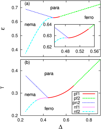
Figure 1: (Color online) Comparison of the canonical and the microcanonical phase diagram. Here, pf1 means first-order para-ferro transition, etc. (a) Phase diagram in the $\Delta$ – $\varepsilon$ plane in the microcanonical ensemble, Eqs. (7) and (8). The two tricritical points are at $\Delta\approx 0.545$, $\varepsilon\approx 0.636$, and at $\Delta\approx 0.477$, $\varepsilon\approx 0.628$, while there is a critical end point at $\Delta\approx 0.487$, $\varepsilon\approx 0.628$. The inset shows a zoom into the central part. (b) Phase diagram in the $\Delta$ – $T$ plane in the canonical ensemble, Eqs. (3) and (4). There are two tricritical points at $\Delta\approx 0.667$, $T\approx 0.333$, and at $\Delta\approx 0.34$, $T\approx 0.267$. The critical end point is at $\Delta\approx 0.441$, $T\approx 0.279$.

While the phase diagrams in Fig. 1 look simple, their mappings onto each other (Fig. 2) reveal nontrivial inequivalence between the canonical and microcanonical descriptions. This inequivalence is because while the self-consistent solutions (3,6) and (7,10) are the same for both the ensembles and transform onto one another by using Eq. (9), they are nevertheless stable in different parameter regimes. Thus, using the mapping, Eq. (9), two situations can arise: either a gap, i.e., a region of inaccessible states, or an overlap, i.e., a region of multiple stable solutions. Note that the second-order transition to the nematic phase is the same in both the descriptions.

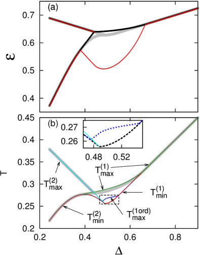
Figure 2: (Color online) Inequivalence of phase diagrams in the two ensembles. (a) Canonical phase diagram Fig. 1(b) mapped onto the $\Delta$ – $\varepsilon$ plane (the microcanonical diagram is in background in gray). Between the bold black and the thin red lines, there is no canonical equilibrium state possible. (b) Microcanonical phase diagram Fig. 1(a) mapped onto the $\Delta$ – $T$ plane (the canonical diagram is in the background in gray). $T^{(1)}_{\rm min}$ (red) is the minimal temperature at which the paramagnetic phase exists. $T^{(1)}_{\rm max}$ (green) is the maximum temperature at which the ferromagnetic phase exists. $T^{(2)}_{\rm max}$ (cyan) (respectively, $T^{(2)}_{\rm min}$ (brown)) is the maximum (respectively, minimum) temperature at which the nematic phase exists. The blue line for $T^{\rm(1ord)}_{\rm max}$ shows the splitting of the first-order microcanonical transition in the region $0.477<\Delta<0.545$ (another line that belongs to this splitting is masked by $T^{(1)}_{\rm min}$ and $T^{(2)}_{\rm min}$). The inset shows a zoom into this middle region, where black dashed and blue dotted lines correspond to the two values of the temperature at the microcanonical jump.

As Fig. 2(a) shows, mapping of the canonical phase diagram onto the $\Delta$ – $\varepsilon$ plane yields a gap. In the domain of $\Delta$ where a first-order canonical transition occurs, the canonical transition line splits into two lines when mapped onto the $\Delta$ – $\varepsilon$ plane. Between these lines, there is no stable canonical state for a given $\varepsilon$ (cf. Fig. 3).

A more nontrivial situation arises due to the mapping of the microcanonical phase diagram onto the $\Delta$ – $T$ plane, as shown in Fig. 2(b). Here, two features are evident. First, in regions where the microcanonical transition is of second order but the canonical transition is of first order, there are three microcanonically stable values of $R_{1,2}$ at temperatures between the lines $T^{(1)}_{\rm max}$ (green line) and $T^{(1)}_{\rm min}$ (red line), and those between the lines $T^{(1)}_{\rm max}$ and $T^{(2)}_{\rm min}$ (brown line). Second, in regions of a first-order microcanonical transition, the transition line splits into two lines, denoted $T^{({\rm 1ord})}_{\rm max}$ (blue line) and $T^{({\rm 1ord})}_{\rm min}$ (black dashed line), with the latter coinciding with either $T^{(1)}_{\rm min}$ or $T^{(2)}_{\rm min}$, such that for temperatures in between, there are two microcanonically stable values of $R_{1,2}$, see the inset of Fig. 2(b) and cuts of the $\Delta$ – $T$ phase diagram at fixed values of $\Delta$ in Fig. 3. Thus, in the whole domain of $\Delta$ where the canonical transition is of first-order, one observes a multiplicity of microcanonically stable states in the $\Delta$ – $T$ plane. Remarkably, the tricritical points are different in the two ensembles.

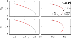
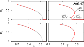
Figure 3: (Color online) Stable solutions of $R_{1,2}$ vs. temperature $T$ in the canonical ensemble and energy $\varepsilon$ in the microcanonical ensemble (dotted grey lines); red solid lines are stable “imports” from another ensemble (canonically stable states on left column panels and microcanonically stable states on right column panels); $\Delta$ equals $0.49$ (top panel), and $0.47$ (bottom panel). The values of $T^{(1)}_{\rm max},T^{(1)}_{\rm min},T^{(2)}_{\rm max},T^{(2)}_{\rm min},T^{({\rm 1ord})}_{\rm max}$ marked by arrows coincide with those in Fig. 2.

In Fig. 4, we employ relation (9) to draw the temperature-energy relation $T(\varepsilon)$ for $\Delta=0.5$. Both for the microcanonical and the canonical ensemble, this curve has two branches: a high-energy branch, and a low-energy branch. At the point where the two branches intersect, the two entropies in the microcanonical ensemble and the two free energies in the canonical ensemble become equal. In the region where the canonical curve shows a jump in the energy at a given temperature, characteristic of a first-order transition that here occurs between the paramagnetic and the ferromagnetic phase (see Fig. 1(b)), the microcanonical curve shows a region of negative specific heat ($\partial T/\partial\varepsilon<0$). Since the canonical specific heat is always positive, being given by the fluctuations in the energy of the system, the negative microcanonical specific heat is a further indication of ensemble inequivalence for the model under study.

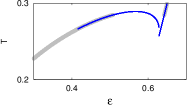
Figure 4: (Color online) Plot of the dependence $\varepsilon$-$T$ for $\Delta=0.5$, showing regions of microcanonical energies that are inaccessible canonically. Bold grey lines: canonically stable states, blue solid lines: microcanonically stable states.

To conclude, we addressed the issue of ensemble inequivalence in long-range interacting systems, by studying an XY model of classical spins with linear and quadratic coupling, and evolving under Hamilton dynamics. In this so-called Generalized Hamiltonian mean-field model, we compared exact equilibrium phase diagrams in the microcanonical and canonical ensembles. We showed that within the region of first-order transitions, the two ensembles show very different behaviors. Nevertheless, let us remark that when plotted using appropriate variables, the arrangement of critical points and transition lines is similar in the phase diagrams of the two ensembles. One may study how the relaxation to equilibrium differs in the two ensembles, a behavior investigated earlier in the microcanonical ensemble in Ref. Teles:2012 . In that paper, it was shown that an isolated system described by the Hamiltonian (1) relaxes to quasi-stationary states (QSSs) which also have paramagnetic, ferromagnetic, and nematic phases. The phase diagram of QSS, however, is very different from the one predicted by the equilibrium statistical mechanics in the microcanonical ensemble, Fig. 1. Nevertheless, we expect that since the life-time of QSS scales with the number of particles in the system, a finite system will eventually relax to the Boltzmann-Gibbs equilibrium. In the thermodynamic limit, however, this relaxation might take longer than the age of the Universe. It will be of interest to explore such dynamical behavior in the canonical ensemble.

Finally, we mention that an overdamped nonequilibrium version of the GHMF is a Kuramoto-type model of synchronization of globally coupled oscillators (just as an overdamped nonequilibrium version of the HMF model is the standard Kuramoto model Gupta:20141 ; Gupta:20142 ), where transitions to synchronization are of major interest. In the context of synchronization, nematic and ferromagnetic phases correspond respectively to two-cluster and one-cluster synchronization patterns (see Ref. Komarov:2013 ), but their stability is obtained from dynamical and not from free energy/entropy considerations.

AP is supported by the grant from the agreement of August 27, 2013, number 02.В.49.21.0003 between the Ministry of Education and Science of the Russian Federation and the Lobachevsky State University of Nizhni Novgorod. SG is supported by the CEFIPRA Project 4604-3. The authors thank the Galileo Galilei Institute for Theoretical Physics, Florence, Italy for the hospitality and the INFN for partial support during the completion of this work. SG and AP acknowledge useful discussions with M. Komarov. This work was partially supported by the CNPq, FAPERGS, INCT-FCx, and by the US-AFOSR under the grant FA9550-12-1-0438.

References

- (1) A. Campa, T. Dauxois and S. Ruffo, Phys. Rep. 480, 57 (2009).
- (2) F. Bouchet, S. Gupta and D. Mukamel, Physica A 389, 4389 (2010).
- (3) Y. Levin, R. Pakter, F. B. Rizzato, T. N. Teles and F. P. C. Benetti, Phys. Rep. 535, 1 (2014).
- (4) A. Campa, T. Dauxois, D. Fanelli and S. Ruffo, Physics of Long-Range Interacting Systems (Oxford University Press, Oxford, 2014).
- (5) J. Sopik, C. Sire and P. H. Chavanis, Phys. Rev. E 72, 026105 (2005).
- (6) D. R. Nicholson, Introduction to Plasma Physics (Krieger Publishing Company, Florida, 1992).
- (7) L. D. Landau and E. M. Lifshitz Electrodynamics of Continuous Media (Pergamon, London, 1960).
- (8) P. H. Chavanis Dynamics and Thermodynamics of Systems with Long-range Interactions (Lecture Notes in Physics vol. 602) edited by T. Dauxois, S. Ruffo, E. Arimondo and M. Wilkens (Springer-Verlag, Berlin, 2002).
- (9) T. Padmanabhan, Phys. Rep. 188, 285 (1990).
- (10) D. Lynden-Bell and R. Wood, Mon. Not. R. Astron. Soc. 138, 495 (1968).
- (11) W. Thirring, Z. Phys. 235, 339 (1970).
- (12) M. K. H. Kiessling and J. L. Lebowitz, Lett. Math. Phys. 42, 43 (1997).
- (13) J. Barré, D. Mukamel and S. Ruffo, Phys. Rev. Lett. 87, 030601 (2001).
- (14) I. Ispolatov and E. G. D. Cohen, Physica A 295, 475 (2001).
- (15) J. Barré and B. Gonçalves, Physica A 386, 212 (2007).
- (16) D. Mukamel, S. Ruffo and N. Schreiber, Phys. Rev. Lett. 95, 240604 (2005).
- (17) A. Venaille and F. Bouchet, Phys. Rev. Lett. 102, 104501 (2009).
- (18) A. Venaille and F. Bouchet, J. Stat. Phys. 143, 346 (2011).
- (19) T. N. Teles, D. Fanelli and Stefano Ruffo, Phys. Rev. E 89, 050101(R) (2014).
- (20) F. Bouchet and J. Barré, J. Stat. Phys. 118 1073 (2005).
- (21) F. Bouchet, T. Dauxois, D. Mukamel and S. Ruffo, Phys. Rev. E 77, 011125 (2008).
- (22) M. Antoni and S. Ruffo, Phys. Rev. E 52, 2361 (1995).
- (23) Y. Y. Yamaguchi, J. Barré, F. Bouchet, T. Dauxois and S. Ruffo, Physica A 337, 36 (2004).
- (24) A. Campa, A. Giansanti and G. Morelli, Phys. Rev. E 76, 041117 (2007).
- (25) M. Joyce and T. Worrakitpoonpon, J. Stat. Mech.: Theory Exp. P10012 (2010).
- (26) D. H. Lee and G. Grinstein, Phys. Rev. Lett. 55, 541 (1985).
- (27) T. N. Teles, F. P. C Benetti, R. Pakter R and Y. Levin, Phys. Rev. Lett. 109, 230601 (2012).
- (28) M. Kac, G. E. Uhlenbeck and P. C. Hemmer, J. Math. Phys. 4, 216 (1963).
- (29) K. Qi, M. H. Qin, X. T. Jia and J.-M. Liu, J. Magn. Magn. Mater., 340, 127 (2013).
- (30) D. B. Carpenter and J. T. Chalker, J. Phys.: Condens. Matter, 1, 4907 (1989)
- (31) J.-H. Park, S. Onoda, N. Nagaosa and J. H. Han, Phys. Rev. Lett., 101, 167202 (2008)
- (32) M. Antoni, S. Ruffo and A. Torcini, Phys. Rev. E 66, 025103(R) (2002).
- (33) M. Komarov and A. Pikovsky, Phys. Rev. Lett. 111, 204101 (2013); Physica D 289, 18 (2014); V. Vlasov, M. Komarov and A. Pikovsky, arXiv:1411.3204.
- (34) S. Gupta, A. Campa and S. Ruffo, Phys. Rev. E 89, 022123 (2014).
- (35) S. Gupta, A. Campa and S. Ruffo, J. Stat. Mech.: Theory Exp. R08001 (2014).