Low temperature dynamics of nonlinear Luttinger liquids

Abstract

We generalize nonlinear Luttinger liquid theory to describe the dynamics of one-dimensional quantum critical systems at low temperatures. Analyzing density-matrix renormalization group results for the spin autocorrelation function in the XXZ chain we provide, in particular, direct evidence for spin diffusion in sharp contrast to the exponential decay in time predicted by conventional Luttinger liquid theory. Furthermore, we discuss how the frequencies and exponents of the oscillatory contributions from the band edges are renormalized by irrelevant interactions and obtain excellent agreement between our finite temperature nonlinear Luttinger liquid theory and the numerical data.

Introduction—The dynamics of quantum critical systems at finite temperatures is an outstanding challenge in many-body physics sachdev . Understanding the combined effects of thermal fluctuations and interactions is crucial for the interpretation of experiments that probe frequency-dependent responses and scattering cross sections. Addressing this problem has become even more pressing since fascinating new experiments in cold atomic gases fukuhara ; hild ; knap ; langen and condensed matter bisogni have given us access to correlation functions directly in the time domain.

Much of the interest in real time evolution of many-body states has focused on one-dimensional (1D) models. In particular, the difference in the nonequilibrium dynamics of integrable versus nonintegrable systems is currently a hotly debated topic kinoshita ; rigol ; cazalilla ; gangardt ; fagotti . In parallel, studies of ground state dynamical correlations have recently forced us to revise our understanding of quasiparticles in critical 1D systems rozhkov ; carmelo ; pustilnik ; pereira2006 ; khodas2007 ; imambekovscience ; furusaki ; matveev , culminating with the development of the nonlinear Luttinger liquid (NLL) theory imambekov . This theory provides a framework for calculating exponents of edge singularities in dynamical response functions based on a picture of fermionic quasiparticles with nonlinear dispersion, reminiscent of elementary excitations in Bethe ansatz (BA) solvable models pereira2008 ; essler10 . NLL theory predicts that the long-time decay of correlation functions is dominated by excitations involving particles or holes near band edges, explaining the high-frequency oscillations observed numerically pereira2008 ; pereira2009 and confirmed by an exact form factor approach kitanine .

The purpose of this Letter is to extend NLL theory to describe the low temperature, long time decay of correlation functions of 1D quantum fluids. Determining the precise effects of temperature is certainly relevant for experiments aimed at testing the phenomenology of NLLs. Another motivation for this work is to provide analytic expressions to examine numerical results for time dependent correlation functions, accessible by finite-temperature versions sirkerklumper ; barthel ; karrasch ; karrasch2 ; barthel2 of time-dependent tdmrg1 ; tdmrg2 ; tdmrg3 ; tdmrg4 ; tdmrg5 density matrix renormalization group (tDMRG) methods white ; dmrgrev , and for the thermal broadening of edge singularities in the frequency domain panfil . In the following we will generalize NLL theory to $T>0$ and compare the predictions with state-of-the-art tDMRG results. We will concentrate on the spin autocorrelation function $G(t)$ of the XXZ model at zero magnetic field, but our approach can easily be generalized to other correlations and 1D models. We stress that the time decay of correlation functions in the XXZ model at finite $T$ is still an open problem despite the integrability of the model korepin ; korepinbook . Our main results are: (i) $G(t)$ at intermediate times $t$ is well described by a generalization of NLL theory that takes into account the effects of irrelevant operators on the dispersion of high-energy quasiparticles and on their coupling to low energy modes; (ii) at long times, $G(t)$ contains a non-oscillating, $\sim 1/\sqrt{t}$ decaying diffusive term, in sharp contrast to the exponential decay predicted by Luttinger liquid theory. Diffusive behavior in spins chains has been invoked to explain the spin-lattice relaxation rate thurber and muon-spin relaxation xiao measured in quasi-1D antiferromagnets and is attributed to inelastic umklapp scattering sirker . However, fingerprints of spin diffusion have so far only been found indirectly in the current-current correlation function sirker ; karrasch ; drudepaper2 and in the imaginary time dependence of the dynamical susceptibility brenig . Here we provide the first direct numerical evidence of spin diffusion in the autocorrelation function.

Model—Consider the 1D XXZ Hamiltonian

$$H=\sum_{j=1}^{L}\left(S_{j}^{x}S_{j+1}^{x}+S_{j}^{y}S_{j+1}^{y}+\Delta S_{j}^{z}S_{j+1}^{z}\right),$$ (1)

where $S_{j}^{a}$ are spin-$1/2$ operators, $\Delta$ is the anisotropy parameter, and periodic boundary conditions are assumed. This model can be realized, for instance, in the Mott insulating phase of two-component Bose mixtures in 1D optical lattices duan ; fukuhara . The spin autocorrelation function at temperature $T$ is defined by

$$G(t)=\langle S^{z}_{j}(t)S^{z}_{j}(0)\rangle=\textrm{Tr}\{S^{z}_{j}(t)S^{z}_{j}(0)e^{-H/T}\}/Z,$$ (2)

where $Z=\textrm{Tr}\,e^{-H/T}$ is the partition function. The XXZ model is equivalent to spinless fermions, $c^{(\dagger)}_{j}$, via a Jordan-Wigner transformation with $S_{j}^{z}\to c_{j}^{\dagger}c^{\phantom{\dagger}}_{j}-1/2$, so that $\Delta$ plays the role of a nearest-neighbor density-density interaction giamarchi .

Noninteracting case—For $\Delta=0$, the XXZ model reduces to a free fermion model. The autocorrelation factorizes into a product of free particle and hole Green’s functions and is given exactly by sirkerprb2006

$$G^{(0)}(t)=\langle c_{j}^{\phantom{\dagger}}(t)c_{j}^{\dagger}(0)\rangle\langle c_{j}^{\dagger}(t)c_{j}^{\phantom{\dagger}}(0)\rangle=\left(\int_{-\pi}^{\pi}\frac{dk}{2\pi}\,f_{k}e^{i\epsilon_{k}t}\right)^{2},$$ (3)

with dispersion $\epsilon_{k}=-\cos k$ and Fermi distribution $f_{k}=1/(e^{\epsilon_{k}/T}+1)$ at half-filling.

Let us discuss an approximation that captures the asymptotic long time decay of $G^{(0)}(t)$. First note that $G^{(0)}(t)$ oscillates at arbitrary temperatures due to saddle points of the integrand where $d\epsilon_{k}/dk=0$, which occur at $k=0$ and $k=\pi$. In the low-temperature regime $T\ll 1$, we employ a mode expansion of the fermion field which keeps only states within sub-bands near the smeared Fermi surface and near the saddle points, in the form $c_{j=x}\sim\psi_{R}(x)e^{i\pi x/2}+\psi_{L}(x)e^{-i\pi x/2}+\bar{d}^{\dagger}(x)+e^{i\pi x}d(x)$. Here $\psi_{R,L}$ are the low-energy right- and left-moving components, while $\bar{d}$ and $d$ are high-energy modes: $\bar{d}^{\dagger}$ creates a hole at the bottom of the band ($k=0$), and $d$ annihilates a particle at the top of the band ($k=\pi$).

The mode expansion reduces the problem to the calculation of free propagators for $\psi_{R,L}$ and $d,\bar{d}$. The low energy modes have linear dispersion, thus their propagator at $T\ll 1$ is given by the standard conformal field theory result $\langle\psi^{\phantom{\dagger}}_{R,L}(x,t)\psi^{\dagger}_{R,L}(x,0)\rangle\sim\pi T/\sinh(\pi Tt)$. On the other hand, the high-energy modes do not feel the temperature, up to an exponentially small correction in the Fermi distribution. Since the dispersion is parabolic near the band edges, $\epsilon_{k}\approx 1-k^{2}/2$, the propagator of $d,\bar{d}$ decays slowly, $\langle d(x,t)d^{\dagger}(x,0)\sim e^{-it}/\sqrt{t}$. Substituting the contributions from low and high energy modes into Eq. (3), we obtain the asymptotic decay of $G^{(0)}(t)$:

$$G^{(0)}(t)\approx\frac{ie^{-i2t}}{2\pi t}+\frac{\sqrt{2}Te^{-i(t+\pi/4)}}{\sqrt{\pi t}\sinh(\pi Tt)}-\frac{T^{2}}{\sinh^{2}(\pi Tt)}.$$ (4)

The first term stems from the contribution in which both particle and hole are high-energy modes. The second term is due to a high-energy particle (hole) plus a low-energy hole (particle) at either one of the Fermi points. The latter decays exponentially for $t\gg 1/T$. The third contribution is due only to the low-energy modes $\psi_{R,L}$, and decays more rapidly than the oscillating terms. Therefore, $G^{(0)}(t)$ for $t\gg 1/T$ is dominated by the term oscillating with frequency $\omega=2$ and decaying as $1/t$.

Interacting case: NLL theory—We focus on the regime $0<\Delta<1$ corresponding to a critical phase of fermions with repulsive interactions. The factorization of $G(t)$ as in Eq. (3) is then a priori lost. However, we can investigate the long time decay of $G(t)$ using the framework of NLL theory imambekov . The idea is to keep the mode expansion with both low and high energy modes, which are now identified as quasiparticles in a renormalized band. The ground state is a vacuum of $d$ and $\bar{d}$, and the spin operator $S_{j}^{z}\sim c^{\dagger}_{j}c_{j}^{\phantom{\dagger}}$ creates at most one $d$ particle and/or one $\bar{d}$ hole. At low temperatures, we neglect an exponentially small thermal population of the band edge modes. The $d,\bar{d}$ quasiparticles can then be treated as mobile “impurities” distinguishable from the low energy modes.

At $T=0$ the dynamics is described by an effective field theory with Hamiltonian density pereira2008

$$\mathcal{H} = d^{\dagger}\left(\varepsilon+\frac{\partial_{x}^{2}}{2m}\right)d+\bar{d}^{\dagger}\left(\varepsilon+\frac{\partial_{x}^{2}}{2m}\right)\bar{d}+Vd^{\dagger}d\,\bar{d}^{\dagger}\bar{d}$$ (5)

$$+ \frac{v}{2}[(\partial_{x}\theta)^{2}+(\partial_{x}\phi)^{2}]+\frac{v\alpha}{\sqrt{\pi K}}\partial_{x}\phi(d^{\dagger}d-\bar{d}^{\dagger}\bar{d}).$$

Here $\varepsilon$ is the energy and $m$ the absolute value of the effective mass of the band edge modes, $V$ is the impurity-impurity interaction, $\phi(x)$ and $\theta(x)$ are dual fields representing the bosonized low-energy modes giamarchi and obey $[\phi(x),\partial_{x^{\prime}}\theta(x^{\prime})]=i\delta(x-x^{\prime})$. $v$ is the spin velocity, $K$ the Luttinger parameter, and $\alpha$ the dimensionless coupling constant of the impurity-boson interaction. For the integrable XXZ model one finds $v=\varepsilon=\frac{1}{m}=\frac{\pi\sqrt{1-\Delta^{2}}}{2\arccos\Delta}$, $K=1-\frac{\alpha}{2\pi}=\frac{\pi/2}{\pi-\arccos\Delta}$, while $V\approx-4\Delta$ for $\Delta\ll 1$.

Eq. (5) must be regarded as a fixed point Hamiltonian which includes all marginal interactions allowed by symmetry. This model can be solved exactly by performing a unitary transformation that decouples the impurities from the bosonic modes, but attaches “string” operators to the $d,\bar{d}$ fields, i.e. $d(x)\to d(x)e^{-i\alpha\theta(x)/\sqrt{\pi K}}$ pustilnik . This allows one to predict the long time decay of $G(t)$ at $T=0$, up to non-universal amplitudes pereira2008 .

We now extend NLL theory to $0<T\ll\varepsilon$ (low temperatures compared to the renormalized bandwidth), using Eq. (5) as a starting point. We obtain the leading $T$ dependence by analyzing the effects of irrelevant interactions. The leading corrections to the oscillating terms in $G(t)$ allowed by symmetry supplem stem from the irrelevant dimension-three operators

$$\delta\mathcal{H} = g[(\partial_{x}\theta)^{2}+(\partial_{x}\phi)^{2}](d^{\dagger}d+\bar{d}^{\dagger}\bar{d})$$ (6)

$$+g^{\prime}[(\partial_{x}\theta)^{2}-(\partial_{x}\phi)^{2}](d^{\dagger}d+\bar{d}^{\dagger}\bar{d})$$

$$-\mu_{+}\partial^{2}_{x}\theta\left(d^{\dagger}d-\bar{d}^{\dagger}\bar{d}\right)$$

$$+\mu_{-}\partial_{x}\theta\left(-id^{\dagger}\partial_{x}d+i\bar{d}^{\dagger}\partial_{x}\bar{d}+h.c.\right).$$

Substituting the mode expansion into Hamiltonian (1) and bosonizing the low-energy modes, we find for $\Delta\ll 1$: $g\approx-\Delta$ , $\mu_{-}\approx-\Delta/\sqrt{\pi}$, while $g^{\prime}$ and $\mu_{+}$ are not generated to first order in $\Delta$. The $g^{\prime}$ interaction is particularly important: it can be identified with a three-body scattering process khodas2007 ; pereira2008 and gives rise to a nonzero impurity decay rate for $T>0$ castroneto ; karzig . However, by imposing nontrivial conservation laws in the XXZ model we can show that $g^{\prime}=0$ exactly supplem ; KluemperSakai , as expected from the lack of three-body scattering in integrable models.

We calculate the impurity self-energy $\Sigma$ and effective impurity-boson interaction $\tilde{\alpha}$ by perturbation theory in the irrelevant operators. The leading $T$ dependence is determined by loop diagrams which contain only one irrelevant coupling constant but arbitrary factors of the bare $\alpha$. In the calculation of loop diagrams, it is convenient to treat the quadratic term in the impurity dispersion (which is also a dimension-three operator) as a perturbation, expanding the internal impurity propagators in powers of $1/m$. We find

$$\Sigma(T)\approx c_{\Sigma}T^{2}/v^{2},\quad\tilde{\alpha}(T)\approx\alpha(1+c_{\alpha}T/v^{2}).$$ (7)

The prefactors $c_{\Sigma}$ and $c_{\alpha}$ are linear functions of $g,\mu_{+},\mu_{-}$. Bearing in mind that $g,\mu_{-}\sim\mathcal{O}(\Delta)$, $\mu_{+}\sim\mathcal{O}(\Delta^{2})$ for $\Delta\ll 1$ , we obtain the weak coupling approximation

$$c_{\Sigma}\approx\frac{\pi g}{3}+\frac{\alpha^{2}}{12Km},\quad c_{\alpha}\approx-2g+\frac{\alpha^{2}}{2\pi Km}.$$ (8)

Omitted terms are $\mathcal{O}(\Delta^{3})$ or higher. To first order in $\Delta$, the self-energy and vertex correction are both governed by $g\approx-\Delta$. For $0<\Delta\ll 1$, Eq. (7) thus implies that the effective impurity energy $\tilde{\varepsilon}(T)=\varepsilon+\Sigma(T)$ decreases $\sim T^{2}$, whereas the effective coupling $\tilde{\alpha}$ increases linearly with $T$. Phenomenologically, we find $g=\frac{\pi v^{2}}{2K}\frac{\partial^{2}\varepsilon}{\partial h^{2}}\big{|}_{h=0}$ relating the coupling constant $g$ in Eq. (6) to a change in the impurity energy when applying a magnetic field $h$. This allows one to obtain $g(\Delta)$ exactly using the BA and Wiener-Hopf techniques. Unfortunately, the corrections of higher order in $\alpha$ in Eq. (7) quickly become of the same order as the $\mathcal{O}(g)$ term making it impossible to fix $c_{\Sigma}$, $c_{\alpha}$ beyond the lowest order in $\Delta$. Importantly however, the $T$ dependence does hold for arbitrary $0<\Delta<1$, as long as the temperature is small enough.

The renormalization of the impurity-impurity interaction appears at order $g^{2}$. The basic process involves a two-boson loop connecting two impurity lines. The correction depends on the momentum and frequency exchange between the impurities: $\tilde{V}(q,\omega,T)\approx V+\frac{2\pi g^{2}T^{2}\omega}{3v^{4}q}$, where we simplified the result in the physically relevant regime $\omega\ll vq$ for impurities with parabolic dispersion.

We can now describe the decay of $G(t)$ using the methods of NLL theory with renormalized parameters at $T>0$. First, consider the contribution from the excitation with a single impurity, equivalent to the second term in Eq. (4). The unitary transformation introduces a “string” operator whose scaling dimension depends on temperature through $\tilde{\alpha}(T)$. The result is

$$G_{1}(t)\approx\frac{A(T)}{\sqrt{t}}\left[\frac{\pi T}{\sinh(\pi Tt)}\right]^{\tilde{\eta}(T)}e^{-i[\tilde{\varepsilon}(T)t+\tilde{\varphi}(T)]},$$ (9)

where $\tilde{\eta}(T)=\frac{K}{2}+\frac{1}{2K}\left[1-\frac{\tilde{\alpha}(T)}{2\pi}\right]^{2}$, $\tilde{\varphi}(T)=\frac{\pi}{2}\left[\tilde{\eta}(T)-\frac{1}{2}\right]$, and $A(T)$ is the unknown prefactor. Note that $\tilde{\alpha}(T)>\alpha$ for $0<\Delta\ll 1$ implies that $\tilde{\eta}(T)$ decreases with temperature, slightly slowing down the decay of $G_{1}(t)$.

The two-impurity contribution to $G(t)$, analogous to the first term in Eq. (4), is strongly modified by the $V$ interaction. At $T=0$, the $1/t$ decay for $\Delta=0$ changes to $1/t^{2}$ for $\Delta>0$ and $t\gg 1/V^{2}$ pereira2008 . This asymptotic behavior is associated with two impurities scattering in a ladder series with small energy and momentum transfer, $\omega\sim q^{2}/m\ll\varepsilon$. Neglecting the renormalization of $V$ for $\omega\ll vq$, we obtain the two-impurity contribution

$$G_{2}(t)\approx\frac{B(T)}{t^{2}}\,e^{-i2\tilde{\varepsilon}(T)t},$$ (10)

where $B(T)$ is the unknown prefactor. For generic models, Eq. (10) must be modified to include the exponential decay due to relaxation by the three-body process $g^{\prime}$.

Diffusive decay—At temperatures $T\ll 1$, conventional Luttinger liquid theory predicts that the non-oscillating terms in $G(t)$, associated only with the low-energy modes $\psi_{R,L}$, are given in the interacting case by $A^{\prime}[\pi T/\sinh(\pi Tt)]^{2}+B^{\prime}[\pi T/\sinh(\pi Tt)]^{2K}$, where the amplitudes $A^{\prime},B^{\prime}$ are known lukyanov . However, we must also consider how irrelevant operators affect the low-energy contributions. In sirker it was shown that the formally irrelevant umklapp scattering

$$\delta\mathcal{H}_{U}=\lambda\cos(4\sqrt{\pi K}\phi)$$ (11)

qualitatively changes the long time decay of the low-energy, long-wavelength contribution to $G(t)$. There appears a new time scale set by the decay rate $\gamma\propto\lambda^{2}T^{8K-3}$. For the XXZ model, $\gamma$ can be calculated exactly lukyanov ; sirker . At low $T$ and long times $t\gg 1/\gamma\gg 1/T$, we find a diffusive contribution

$$G_{\textrm{diff}}(t)=\frac{\Gamma}{\sqrt{t}}\quad,\quad\Gamma=\frac{KT}{\pi v^{2}}\sqrt{\frac{\gamma}{2\pi}}.$$ (12)

Strikingly, this diffusive ($\sim 1/\sqrt{t}$) decay in the autocorrelation function coexists with ballistic transport sirker ; prosen . Eqs. (9, 12) are the two contributions to $G(t)$ which are dominant at intermediate and long times, respectively.

Numerical results—In order to test our theory, we now turn to a comparison with tDMRG results for finite system size. Non-zero temperatures are incorporated via a purification of the density matrix. By using the disentangler introduced in Ref. karrasch and exploiting time translation invariance $\langle S^{z}_{j}(t)S^{z}_{j}(0)\rangle=\langle S^{z}_{j}(t/2)S^{z}_{j}(-t/2)\rangle$ barthel2 we can substantially extend the accessible time scale. Details of the algorithm are described in Refs. karrasch2 ; dmrgrev . By varying both the system size and the bound for the maximally discarded weight we ensure that the finite size and truncation errors are smaller than the symbol size for all data presented in the following.

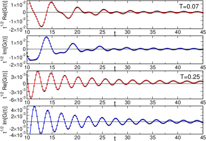
Figure 1: $\sqrt{t}G(t)$ at $\Delta=0.3$: tDMRG data (symbols) and fits (lines) for $t\geq 10$. Here $\lim_{t\to\infty}\sqrt{t}G(t)=\Gamma$ with $\Gamma_{\textrm{fit}}(T=0.07)\approx 0$ [$\Gamma_{\textrm{th}}(T=0.07)=2.1\cdot 10^{-5}$] and $\Gamma_{\textrm{fit}}(T=0.25)\approx 6.3\cdot 10^{-4}$ [$\Gamma_{\textrm{th}}(T=0.25)=7.9\cdot 10^{-4}$].

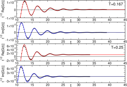
Figure 2: Same as Fig. 1 for $\Delta=0.8$ with $\Gamma_{\textrm{fit}}(T=0.167)\approx 3.3\cdot 10^{-4}$ [$\Gamma_{\textrm{th}}(T=0.167)=5.6\cdot 10^{-4}$] and $\Gamma_{\textrm{fit}}(T=0.25)\approx 9.9\cdot 10^{-4}$ [$\Gamma_{\textrm{th}}(T=0.25)=1.3\cdot 10^{-3}$].

We find a striking difference between the weakly interacting case, Fig. 1, and the strongly interacting case, Fig. 2. While the data for $\Delta=0.8$ can be very well fitted by a sum of the single impurity contribution (9) and the diffusive part (12), it is necessary to also include the two-impurity contribution (10) for $\Delta=0.3$. In the latter case, we also allow for a decay rate $\rho$ by multiplying Eq. (10) by $e^{-\rho t}$. The fits yield very small decay rates which seem to be of order $\sim\text{e}^{-1/T}$ and could possibly be related to thermal excitations at the band edges which we have neglected in our analysis supplem . At $T=0.25$ we find for both $\Delta$ values clear evidence for spin diffusion with diffusion constants $\Gamma_{\textrm{fit}}$ close to the theoretically predicted values, $\Gamma_{\textrm{th}}$, see Eq. (12). In agreement with theory we also find numerically that the diffusive contribution seems to vanish for magnetic fields $h\gg T$ (data not shown) where the Umklapp term (11) is oscillating and should be dropped from the effective theory sirker . The oscillation frequency $\tilde{\varepsilon}(T)$ and exponent $\tilde{\eta}(T)$, obtained from fits of tDMRG data at $\Delta=0.3$, are shown in Fig. 3.

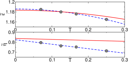
Figure 3: $\tilde{\varepsilon}(T)$ and $\tilde{\eta}(T)$ for $\Delta=0.3$ from fits of tDMRG data (symbols). Dashed lines: quadratic and linear least square fits, respectively; solid lines: $\mathcal{O}(\Delta)$ theoretical result, Eq. (7).

The data confirm that $\tilde{\varepsilon}\sim-T^{2}$ and $\tilde{\eta}\sim-T$ while the prefactors, even for $\Delta=0.3$, already seem to deviate significantly from the lowest order result, Eq. (8).

Exact parameters—The integrability of the XXZ model raises the question whether parameters such as the frequency $\tilde{\varepsilon}(T)$ can be determined exactly, beyond the lowest order in Eq. (7). At $T=0$ the exact $\varepsilon$ is identified with the half bandwidth of the elementary excitations computable by BA pereira2008 . The natural extension to $T>0$ should be based on the energies of excitations on top of an equilibrium state in the thermodynamic Bethe ansatz (TBA) approach takahashi72 ; puga . However, by solving TBA nonlinear integral equations numerically supplem we find that the bandwidth of the dressed energy for a single-hole excitation increases with $T$, whereas the perturbative expression (7) and the tDMRG results in Fig. 3 show that $\tilde{\varepsilon}(T)$ decreases with $T$. This disagreement is rather puzzling given that a generalized TBA approach has been shown to be applicable even to nonequilibrium dynamics caux .

Conclusion—Finite temperatures and quantum fluctuations lead to large non-perturbative effects on dynamical correlations in NLL’s. The exponents of oscillating contributions are renormalized by temperature while umklapp scattering leads to spin diffusion dominating the long-time asymptotics. These predictions are in excellent agreement with tDMRG calculations which provide, in particular, the first direct evidence for spin diffusion in the XXZ model and show striking changes in the one- and two-impurity contributions as a function of temperature and interaction strength. The theory is easily extended to models such as the Bose gas and can also be used to study the propagation of an impurity through a 1D quantum fluid at finite temperatures. We expect, in particular, that these results will help to set up and interpret experiments in ultracold atoms aiming at an observation of spin diffusion knap ; hild .

We thank F.H.L. Essler, L.I. Glazman, A. Klümper and M. Panfil for helpful discussions. J.S. acknowledges support by the Collaborative Research Centre SFB/TR49, the Graduate School of Excellence MAINZ (DFG, Germany), as well as NSERC (Canada). R.G.P. acknowledges support by CNPq (Brazil). C.K. acknowledges support by Nanostructured Thermoelectrics program of LBNL.

Supplemental Material:
“Low temperature dynamics of nonlinear Luttinger liquids”
by C. Karrasch, R. G. Pereira, and J. Sirker

.1 1. Irrelevant impurity-boson interactions

In this section we discuss how discrete symmetries and integrability of the XXZ model constrain the coupling constants of irrelevant operators in the effective impurity model.

Particle-hole ($C$) and parity ($P$) transformations act on the bosonic fields and impurity fields as follows lukyanov :

$$C:\left\{\begin{array}[]{ccc}\theta&\to&-\theta\\ \phi&\to&-\phi\\ d&\to&\bar{d}\\ \bar{d}&\to&d\end{array}\right.\quad,\quad P:\left\{\begin{array}[]{ccc}x&\to&-x\\ \theta&\to&\theta\\ \phi&\to&-\phi\\ d&\to&d\\ \bar{d}&\to&\bar{d}\end{array}\right..$$ (1)

The Hamiltonian can only contain operators that are invariant under $C$ and $P$. Let us denote by $H_{a}^{(n)}=\int dx\,\mathcal{H}_{a}^{(n)}(x)$, $a=1,2,\dots$, a particular term in the Hamiltonian such that $\mathcal{H}_{a}^{(n)}$ is an operator with scaling dimension $n$. Up to dimension four, we have a list of 14 operators allowed by symmetry:

$$\mathcal{H}_{1}^{(2)} = \frac{v}{2}\left[(\partial_{x}\theta)^{2}+(\partial_{x}\phi)^{2}\right],$$

$$\mathcal{H}_{2}^{(1)} = \varepsilon\left(d^{\dagger}d+\bar{d}^{\dagger}\bar{d}\right),$$

$$\mathcal{H}_{3}^{(3)} = -\frac{1}{2m}\left(\partial_{x}d^{\dagger}\partial_{x}d+\partial_{x}\bar{d}^{\dagger}\partial_{x}\bar{d}\right),$$

$$\mathcal{H}_{4}^{(2)} = \frac{v\alpha}{\sqrt{\pi K}}\partial_{x}\phi\left(d^{\dagger}d-\bar{d}^{\dagger}\bar{d}\right),$$

$$\mathcal{H}_{5}^{(2)} = -Vd^{\dagger}d\bar{d}^{\dagger}\bar{d},$$

$$\mathcal{H}_{6}^{(3)} = g\left[(\partial_{x}\theta)^{2}+(\partial_{x}\phi)^{2}\right]\left(d^{\dagger}d+\bar{d}^{\dagger}\bar{d}\right),$$

$$\mathcal{H}_{7}^{(3)} = g^{\prime}\left[(\partial_{x}\theta)^{2}-(\partial_{x}\phi)^{2}\right]\left(d^{\dagger}d+\bar{d}^{\dagger}\bar{d},\right)$$ (2)

$$\mathcal{H}_{8}^{(3)} = \mu_{+}\partial_{x}\theta\,\partial_{x}\left(d^{\dagger}d-\bar{d}^{\dagger}\bar{d}\right),$$

$$\mathcal{H}_{9}^{(3)} = -i\mu_{-}\partial_{x}\theta\left(d^{\dagger}\partial_{x}d-\partial_{x}d^{\dagger}d-\bar{d}^{\dagger}\partial_{x}\bar{d}+\partial_{x}\bar{d}^{\dagger}\bar{d}\right),$$

$$\mathcal{H}_{10}^{(4)} = \vartheta_{+}\left(d^{\dagger}\partial_{x}d\partial_{x}d^{\dagger}d+\bar{d}^{\dagger}\partial_{x}\bar{d}\partial_{x}\bar{d}^{\dagger}\bar{d}\right),$$

$$\mathcal{H}_{11}^{(4)} = \vartheta_{-}\left(d^{\dagger}\partial_{x}d-\partial_{x}d^{\dagger}d\right)\left(\bar{d}^{\dagger}\partial_{x}\bar{d}-\partial_{x}\bar{d}^{\dagger}\bar{d}\right),$$

$$\mathcal{H}_{12}^{(4)} = i\kappa_{1}\partial_{x}^{2}\phi\left(d^{\dagger}\partial_{x}d-\partial_{x}d^{\dagger}d-\bar{d}^{\dagger}\partial_{x}\bar{d}+\partial_{x}\bar{d}^{\dagger}\bar{d}\right),$$

$$\mathcal{H}_{13}^{(4)} = i\kappa_{2}\partial_{x}\phi\partial_{x}\theta\left(d^{\dagger}\partial_{x}d-\partial_{x}d^{\dagger}d+\bar{d}^{\dagger}\partial_{x}\bar{d}-\partial_{x}\bar{d}^{\dagger}\bar{d}\right),$$

$$\mathcal{H}_{14}^{(4)} = \kappa_{3}\partial_{x}\phi\left(\partial_{x}d^{\dagger}\partial_{x}d-\partial_{x}\bar{d}^{\dagger}\partial_{x}\bar{d}\right).$$

All the operators in Eq. (2) conserve the total number of particles and holes in the high-energy subbands. In the above list we have omitted operators which couple the impurity modes to umklapp type operators. The lowest dimension operator in this family is $(d^{\dagger}d+\bar{d}^{\dagger}\bar{d})\cos(4{\sqrt{\pi K}\phi})$, whose scaling dimension varies continuously from $5$ at $\Delta=0$ to $3$ at $\Delta=1$. The set of constraints on the coupling constants that we shall derive in the following is not affected by this family of operators.

The integrability of the XXZ model affects the effective impurity model by constraining the coupling constants of irrelevant interactions. Following pereira2006 , we shall examine the consequences of integrability by imposing the existence of nontrivial conservation laws. For the XXZ model, it is fortunate that the first nontrivial conserved quantity can be identified with the energy current operator $J_{E}$, which is defined from the continuity equation for the Hamiltonian density KluemperSakai . In the continuum limit, the energy current density is given by

$$\partial_{x}j(x)=i[\mathcal{H}(x),H],$$ (3)

where $H=\int dx\,\mathcal{H}(x)=\sum_{a}\int dx\,\mathcal{H}_{a}$ is the total Hamiltonian. The energy current operator is $J_{E}=\int dx\,j(x)$. Let us denote by $j_{a,b}$, with $a<b$, the contribution to the energy current density obtained by taking the commutator of terms $\mathcal{H}_{a}$ and $\mathcal{H}_{b}$ in the Hamiltonian as follows:

$$\partial_{x}j_{a,b}^{(n+m-2)}=i\int dy\,\left\{\left[\mathcal{H}_{a}^{(n)}(x)\mbox{,}\mathcal{H}_{b}^{(m)}(y)\right]+\left[\mathcal{H}_{b}^{(m)}(x)\mbox{,}\mathcal{H}_{a}^{(n)}(y)\right]-\delta_{ab}\left[\mathcal{H}_{a}^{(n)}(x)\mbox{,}\mathcal{H}_{a}^{(n)}(y)\right]\right\}.$$ (4)

The notation implies that when we take the commutator of a dimension-$n$ operator with another dimension-$m$ operator, the corresponding contribution to $J_{E}$ (when nonvanishing) has dimension $n+m-2$.

To check that $J_{E}=\sum_{a<b}J_{a,b}$ is conserved, we need to take the commutator with all the terms in $H$ again:

$$\left[J_{a,b}^{(n+m-2)},H_{c}^{(l)}\right]=\int dx\,\mathcal{O}_{a,b,c}^{(n+m+l-1)}(x).$$ (5)

We organize the expansion by operator dimension. In order to find nontrivial relations between the coupling constants in Eq. (2), it suffices to compute $[J_{E},H]$ to the level of dimension-four operators. For this we need to consider up to dimension-three operators in $J_{E}$. We find the following list of operators

$$j_{1,1}^{(2)} = -v^{2}\partial_{x}\theta\partial_{x}\phi$$

$$j_{2,3}^{(2)} = \frac{i\varepsilon}{m}\left(d^{\dagger}\partial_{x}d+\bar{d}^{\dagger}\partial_{x}\bar{d}\right)$$

$$j_{1,4}^{(2)} = -\frac{\alpha v^{2}}{\sqrt{\pi K}}\partial_{x}\theta\left(d^{\dagger}d-\bar{d}^{\dagger}\bar{d}\right)$$

$$j_{3,4}^{(3)} = \frac{i\alpha v}{2m\sqrt{\pi K}}\partial_{x}\phi\left(d^{\dagger}\partial_{x}d-\partial_{x}d^{\dagger}d-\bar{d}^{\dagger}\partial_{x}\bar{d}+\partial_{x}\bar{d}^{\dagger}\bar{d}\right)$$

$$j_{3,5}^{(3)} = -\frac{iV}{2m}\left[\bar{d}^{\dagger}\bar{d}\left(d^{\dagger}\partial_{x}d-\partial_{x}d^{\dagger}d\right)+d^{\dagger}d\left(\bar{d}^{\dagger}\partial_{x}\bar{d}-\partial_{x}\bar{d}^{\dagger}\bar{d}\right)\right]$$

$$j_{1,6}^{(3)} = -4gv\partial_{x}\theta\partial_{x}\phi\left(d^{\dagger}d+\bar{d}^{\dagger}\bar{d}\right)$$

$$j_{1,8}^{(3)} = -\mu_{+}v\partial_{x}\phi\partial_{x}\left(d^{\dagger}d-\bar{d}^{\dagger}\bar{d}\right)$$

$$j_{1,9}^{(3)} = i\mu_{-}v\partial_{x}\phi\left(d^{\dagger}\partial_{x}d-\partial_{x}d^{\dagger}d-\bar{d}^{\dagger}\partial_{x}\bar{d}+\partial_{x}\bar{d}^{\dagger}\bar{d}\right)$$ (6)

$$j_{2,9}^{(2)} = 2\mu_{-}\varepsilon\partial_{x}\theta\left(d^{\dagger}d-\bar{d}^{\dagger}\bar{d}\right)$$

$$j_{4,9}^{(3)} = \frac{2\mu_{-}\alpha v}{\sqrt{\pi v}}\partial_{x}\theta\partial_{x}\phi\left(d^{\dagger}d+\bar{d}^{\dagger}\bar{d}\right)-\frac{i\mu_{-}\alpha v}{\sqrt{\pi v}}\left[d^{\dagger}d\left(\bar{d}^{\dagger}\partial_{x}\bar{d}-\partial_{x}\bar{d}^{\dagger}\bar{d}\right)+(d\leftrightarrow\bar{d})\right]$$

$$j_{2,11}^{(3)} = 2i\vartheta_{-}\varepsilon\left[d^{\dagger}d\left(\bar{d}^{\dagger}\partial_{x}\bar{d}-\partial_{x}\bar{d}^{\dagger}\bar{d}\right)+(d\leftrightarrow\bar{d})\right]$$

$$j_{2,12}^{(3)} = 2\kappa_{1}\varepsilon\partial_{x}\phi\partial_{x}\left(d^{\dagger}d-\bar{d}^{\dagger}\bar{d}\right)$$

$$j_{2,13}^{(3)} = -2\kappa_{2}\varepsilon\partial_{x}\theta\partial_{x}\phi\left(d^{\dagger}d+\bar{d}^{\dagger}\bar{d}\right)$$

$$j_{2,14}^{(3)} = -i\kappa_{3}\varepsilon\partial_{x}\phi\left(d^{\dagger}\partial_{x}d-\partial_{x}d^{\dagger}d-\bar{d}^{\dagger}\partial_{x}\bar{d}+\partial_{x}\bar{d}^{\dagger}\bar{d}\right).$$

The calculation of the commutators in Eq. (5) is tedious but straightforward. To simplify the result, we use the known relations for the XXZ model $\varepsilon=1/m=v$. We find that the conservation law $[J_{E},H]=0$ imposes the constraints

$$g = -\frac{V}{4},$$ (7)

$$g^{\prime} = 0,$$ (8)

$$\mu_{-} = -\frac{\alpha v}{2\sqrt{\pi K}},$$ (9)

$$\mu_{+} = 2\kappa_{1},$$ (10)

$$\kappa_{2} = -\frac{\alpha^{2}v}{2\pi K},$$ (11)

$$\kappa_{3} = 0.$$ (12)

Most importantly, integrabiliy rules out the $g^{\prime}$ interaction. This is precisely the operator considered in castroneto which accounts for a finite decay rate of a mobile impurity in a Luttinger liquid at finite temperatures.

.2 2. Excitation energies from the thermodynamic Bethe ansatz

In this section we describe the calculation of dressed energies using the thermodynamic Bethe ansatz (TBA) approach to the XXZ model takahashi72 ; takahashi .

Bethe ansatz states are parametrized by a set of rapidities $\{x_{j}^{\alpha}\}$ which satisfy the Bethe equations. Here $j$ labels the type of string and $\alpha$ specifies a particular rapidity. More precisely, $x_{j}^{\alpha}$ refers to the real part of the rapidity, since the imaginary part is fixed by the string hypothesis takahashi72 ; takahashi . Strings with length $n_{j}>1$ are interpreted as bound states of $n_{j}$ particles. For simplicity, we choose the anisotropy parameter to be $\Delta=\cos(\pi/\nu)$, with $\nu\in\mathbb{Z}$. In this case, we can restrict ourselves to a finite number of strings $j=1,2,\dots,\nu$. The strings with $j=1,2,\dots,\nu-1$ have length $n_{j}=j$ and parity $\upsilon_{j}=+1$; the string with $j=\nu$ has length $n_{\nu}=1$ and parity $\upsilon_{\nu}=-1$.

The Bethe equations (in logarithmic form) for a chain of length $N$ and periodic boundary conditions read

$$Nt_{j}(x_{\alpha}^{j})=2\pi I_{\alpha}^{j}+\sum_{k=1}^{\nu}\sum_{\beta=1}^{M_{k}}\Theta_{jk}(x_{\alpha}^{j}-x_{\beta}^{k}),\qquad\alpha=1,\dots,M_{j},$$ (13)

where $M_{j}$ is the number of strings of type $j$ in the Bethe ansatz state and $I_{\alpha}^{j}$ are integers (for $M_{j}$ odd) or half-integers (for $M_{j}$ even). A particular Bethe ansatz wave function is determined by the set of $I_{\alpha}^{j}$’s. The functions $t_{j}(x)$ and the scattering phase shifts $\Theta_{jk}(x)$ are given by

$$t_{j}(x) = f(x;n_{j},v_{j}),$$ (14)

$$\Theta_{jk}(x) = f(x;|n_{j}-n_{k}|,v_{j}v_{k})+f(x;n_{j}+n_{k},v_{j}v_{k})+2\sum_{l=1}^{\textrm{Min}(n_{j},n_{k})-1}f(x;|n_{j}-n_{k}|+2l,v_{j}v_{k}),$$ (15)

where we define the function

$$f(x;n,v)=\left\{\begin{array}[]{cc}0\,,&\textrm{ if }n/\nu\in\mathbb{Z},\\ 2v\arctan\left[(\cot(n\pi/2\nu))^{v}\tanh(\pi x/2\nu)\right],&\textrm{otherwise}.\end{array}\right.$$ (16)

In the TBA approach, we take the limit $N\to\infty$ and characterize the macroscopic state by the density of particles $\rho(x)$ and density of holes $\rho^{h}(x)$ in rapidity space. The equilibrium state is obtained by minimizing the free energy as a functional of $\rho(x)$ and $\rho^{h}(x)$. This leads to a set of coupled nonlinear integral equations for the dressed energies

$$\varepsilon_{j}(x)=-2\nu\sin(\pi/\nu)a_{j}(x)+\frac{1}{\beta}\sum_{k=1}^{\nu}\upsilon_{k}\int_{-\infty}^{+\infty}dy\,T_{jk}(x-y)\ln[1+e^{-\beta\varepsilon_{k}(y)}],$$ (17)

where $\beta=1/T$ is the inverse temperature and

$$a_{j}(x) = \frac{1}{2\pi}\frac{dt_{j}}{dx},$$ (18)

$$T_{jk}(x) = \frac{1}{2\pi}\frac{d\Theta_{jk}}{dx}.$$ (19)

Eq. (17) can be solved numerically by iteration. In the limit $T\to 0$, the dressed energy for $j=1$ (the even-parity one-string) reduces to the dispersion of the single-hole excitation over the ground state.

The dressed energies can be used to calculate the free energy and other thermodynamic properties takahashi . They also show up as the energies of elementary excitations over the equilibrium state korepin . The thermal excitation spectrum for the gapless phase of the XXZ model was calculated by Puga puga . The energy required to create a single hole with rapidity $x$ in the density of type-$j$ strings is

$$\Delta E_{j}(x)=-\varepsilon_{j}(x)+\frac{1}{\beta}\sum_{k=1}^{\nu}\frac{\Theta_{kj}(\infty)}{\pi}\ln[1+e^{-\beta\varepsilon_{k}(\infty)}].$$ (20)

Notice that the excitation energies $\Delta E_{j}(x)$ differ from the dressed energies in Eq. (17) by a constant term that involves all strings.

Fig. 4 shows the excitation energy for the $j=1$ string for three different values of temperature. We are particularly interested in the bandwidth, which is given by $\Delta E_{1}(0)$. At $T=0$, the bandwidth is known analytically, $\lim_{T\to 0}\Delta E_{1}(0)=\frac{\pi\sqrt{1-\Delta^{2}}}{2\arccos\Delta}$. The important point is that the bandwidth calculated from the TBA dressed energies increases with temperature, contrary to the behavior of the frequencies predicted by the effective field theory and observed numerically using a tDMRG algorithm.

Figure 4: Energy of single one-string excitation as a function of rapidity $x$ for $\Delta=0.5$ and three different values of temperature. From bottom to top: $T=10^{-3}$, $T=0.25$, and $T=5$.

.3 3. Fits of the DMRG data

We have fitted the tDMRG data using the fit function

$$\sqrt{t}G(t)=\Gamma+A\left(\frac{\pi T}{\sinh(\pi Tt)}\right)^{\tilde{\eta}}\text{e}^{-i(\tilde{\varepsilon}t+\tilde{\varphi})}+B\,t^{-3/2}\text{e}^{-2i\tilde{\varepsilon}t}\text{e}^{-\rho t}$$ (21)

where $A,B,\tilde{\eta},\tilde{\varepsilon},\tilde{\varphi},\rho,\Gamma$ are real fitting parameters. The first, constant term $\Gamma$ is the diffusive contribution. The second term is the single impurity contribution, Eq. (9) in the main text, while the third term represents the two-impurity contribution, Eq. (10), where we have allowed for a small decay rate which seems to be of order $\sim\text{e}^{-1/T}$ and might possibly be related to thermal excitations at the band edges. In table 1 we present the fit parameters for the fits shown in Fig. 2 and Fig. 3 of the main text.

	$\Delta$	$T$	$t$ fit range	$\Gamma$	$A$	$\tilde{\eta}$	$\tilde{\varepsilon}$	$\tilde{\varphi}$	$B$	$\rho$
theory	0.3	0	—	0	—	0.838	1.1835	0.530	—	—
theory, $\mathcal{O}(\Delta)$	0.3	0.07	—	$2.11\cdot 10^{-5}$	—	0.831	1.1825	0.520	—	—
fit	0.3	0.07	$t\geq 10$	$\sim 0$	0.275	0.796	1.185	0.751	-0.202	0
theory, $\mathcal{O}(\Delta)$	0.3	0.25	—	$7.94\cdot 10^{-4}$	—	0.814	1.1709	0.493	—	—
fit	0.3	0.25	$t\geq 10$	$6.3\cdot 10^{-4}$	0.421	0.713	1.165	1.990	-0.242	0.016
theory	0.8	0	—	0	—	0.629	1.465	0.202	—	—
theory, $\mathcal{O}(\Delta)$	0.8	0.167	—	$5.58\cdot 10^{-4}$	—	0.533	1.457	0.052	—	—
fit	0.8	0.167	$t\geq 15$	$3.26\cdot 10^{-4}$	0.161	0.403	1.503	-0.238	0	—
theory, $\mathcal{O}(\Delta)$	0.8	0.25	—	$1.26\cdot 10^{-3}$	—	0.492	1.448	-0.013	—	—
fit	0.8	0.25	$t\geq 15$	$9.88\cdot 10^{-4}$	0.210	0.387	1.525	-0.397	0	—

Table 1: Parameters obtained by fitting the tDMRG data presented in the main text, see Figs. 2, 3.

One of our main findings based on the analysis of the numerical data is that the two-impurity contribution becomes very small for large interaction strengths leading to a fit parameter $B$ for $\Delta=0.8$ which is essentially zero. To further support that $B$ for the considered temperatures is strongly reduced with interaction, we present in Fig. 5 below tDMRG data and fits for intermediate interaction strength $\Delta=0.5$.

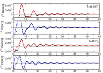
Figure 5: $\sqrt{t}G(t)$ at $\Delta=0.5$: tDMRG data (symbols) and fits (lines) for $t\geq 15$. The fit parameters are given in table 2.

Here a two-impurity contribution is still visible but the amplitude $B$ is already very small, see table 2. In order to illustrate the sensitivity of the fit parameters on the fit interval we concentrate on the case $\Delta=0.5$, $T=0.167$ and show in table 2 parameters for fits using three different time intervals.

	$\Delta$	$T$	$t$ fit range	$\Gamma$	$A$	$\tilde{\eta}$	$\tilde{\varepsilon}$	$\tilde{\varphi}$	$B$	$\rho$
theory	0.5	0	—	0	—	3/4	1.30	0.393	—	—
theory, $\mathcal{O}(\Delta)$	0.5	0.167	—	$3.98\cdot 10^{-4}$	—	0.710	1.2919	0.329	—	—
fit 1	0.5	0.167	$t\geq 10$	$1.68\cdot 10^{-4}$	0.277	0.575	1.294	0.853	-0.086	0.019
fit 2	0.5	0.167	$t\geq 15$	$1.49\cdot 10^{-4}$	0.199	0.527	1.287	1.406	-0.099	0.020
fit 3	0.5	0.167	$t\geq 20$	$1.51\cdot 10^{-4}$	0.284	0.558	1.285	1.853	-0.093	0.019
theory, $\mathcal{O}(\Delta)$	0.5	0.25	—	$1.09\cdot 10^{-3}$	—	0.690	1.2829	0.299	—	—
fit	0.5	0.25	$t\geq 15$	$7.19\cdot 10^{-4}$	0.266	0.501	1.272	2.196	-0.091	0.041

Table 2: Parameters for various fits of the tDMRG data at $\Delta=0.5$.

Except for the phase shift $\tilde{\varphi}$, and, to a lesser extent, the amplitude $\tilde{A}$, all fit parameters show little variation implying, in particular, that it is possible to extract the temperature dependence of $\tilde{\varepsilon}(T)$ and $\tilde{\eta}(T)$ with reasonably accuracy from the tDMRG data. On the other hand, we want to emphasize that the phase shift $\tilde{\varphi}$ cannot be fixed reliably from numerical data even at zero temperature, see Refs. pereira2008 ; pereira2009 .

References

- (1) S. Sachdev, Quantum Phase Transitions (Cambridge University Press, Cambridge, England, 1999).
- (2) T. Fukuhara et al., Nat. Phys. 9, 235 (2013).
- (3) M. Knap, A. Kantian, T. Giamarchi, I. Bloch, M. D. Lukin, and E Demler, Phys. Rev. Lett. 111, 147205 (2013).
- (4) T. Langen, R. Geiger, M. Kuhnert, B. Rauer, and J. Schmiedmayer, Nat. Phys. 9, 640 (2013).
- (5) S. Hild et al., arXiv:1407.6934.
- (6) V. Bisogni et al., Phys. Rev. Lett. 112, 147401 (2014).
- (7) T. Kinoshita et al., Nature (London) 440, 900 (2006).
- (8) M. Rigol, V. Dunjko, V. Yurovsky, and M. Olshanii, Phys. Rev. Lett. 98, 050405 (2007).
- (9) M. A. Cazalilla, Phys. Rev. Lett. 97, 156403 (2006).
- (10) D. M. Gangardt and M. Pustilnik, Phys. Rev. A 77, 041604(R) (2008).
- (11) P. Calabrese, F. H. L. Essler, and M. Fagotti, Phys. Rev. Lett. 106, 227203 (2011).
- (12) A. Rozhkov, Eur. Phys. J. B 47, 193 (2005).
- (13) J. M. P. Carmelo, K. Penc, and D. Bozi, Nucl. Phys. B 725, 421 (2005); Nucl. Phys. B (erratum) 737, 351 (2006).
- (14) M. Pustilnik, M. Khodas, A. Kamenev, and L. I. Glazman, Phys. Rev. Lett. 96, 196405 (2006).
- (15) R. G. Pereira, J. Sirker, J.-S. Caux, R. Hagemans, J. M. Maillet, S. R. White, and I Affleck, Phys. Rev. Lett. 96, 257202 (2006); J. Stat. Mech. P08022 (2007).
- (16) M. Khodas, M. Pustilnik, A. Kamenev, and L. I. Glazman, Phys. Rev. B 76, 155402 (2007).
- (17) A. Imambekov and L. I. Glazman, Science 323, 228 (2009).
- (18) K. A. Matveev and A. Furusaki, Phys. Rev. Lett. 111, 256401 (2013).
- (19) M. Pustilnik and K. A. Matveev, Phys. Rev. B 89, 100504(R) (2014).
- (20) A. Imambekov, T. L. Schmidt, and L. I. Glazman, Rev. Mod. Phys. 84, 1253 (2012).
- (21) R. G. Pereira, S. R. White, and I. Affleck, Phys. Rev. Lett. 100, 027206 (2008).
- (22) F. H. L. Essler, Phys. Rev. B 81, 205120 (2010).
- (23) R. G. Pereira, S. R. White, and I. Affleck, Phys. Rev. B 79, 165113 (2009).
- (24) N. Kitanine, K. K. Kozlowski, J. M. Maillet, N. A. Slavnov and V. Terras, J. Stat. Mech. P09001 (2012).
- (25) J. Sirker and A. Klümper, Phys. Rev. B 71, 241101(R), (2005).
- (26) T. Barthel, U. Schollwöck, and S. R. White, Phys. Rev. B 79, 245101 (2009).
- (27) C. Karrasch, J. Bardarson, and J. Moore, Phys. Rev. Lett. 108, 227206 (2012).
- (28) C. Karrasch, J. Bardarson, and J. Moore, New J. Phys. 15, 083031 (2013).
- (29) T. Barthel, U. Schollwöck, and S. Sachdev, arXiv:1212.3570.
- (30) G. Vidal, Phys. Rev. Lett. 93 040502 (2004).
- (31) S. R. White and A. E. Feiguin, Phys. Rev. Lett. 93 076401 (2004).
- (32) A. Daley, C. Kollath, U. Schollwöck, and G. Vidal, J. Stat. Mech. (2004) P04005.
- (33) P. Schmitteckert, Phys. Rev. B 70 121302(R) (2004).
- (34) M. C. Bañuls, M. B. Hastings, F. Verstraete, and J. I. Cirac, Phys. Rev. Lett. 102 240603 (2009).
- (35) S. R. White, Phys. Rev. Lett 69 2863 (1992).
- (36) U. Schollwöck, Ann. Phys. 326, 96 (2011).
- (37) M. Panfil and J.-S. Caux, Phys. Rev. A 89, 033605 (2014).
- (38) V. E. Korepin and O. I. Patu, PoSSolvay:006 (2006).
- (39) V. E. Korepin, N. M. Bogoliubov and A. G. Izergin, Quantum Inverse Scattering Method and Correlation Functions, Cambridge University Press (1993).
- (40) K. R. Thurber, A. W. Hunt, T. Imai, and F. C. Chou, Phys. Rev. Lett. 87, 247202 (2001).
- (41) F. Xiao et al., arXiv:1406.3202.
- (42) J. Sirker, R. G. Pereira, and I. Affleck, Phys. Rev. Lett. 103, 216602 (2009); Phys. Rev. B 83, 035115 (2011).
- (43) C. Karrasch, J. Hauschild, S. Langer, and F. Heidrich-Meisner, Phys. Rev. B 87 245128 (2013).
- (44) S. Grossjohann and W. Brenig, Phys. Rev. B 81, 012404 (2010).
- (45) L.-M. Duan, E. Demler, and M. D. Lukin, Phys. Rev. Lett. 91, 090402 (2003).
- (46) T. Giamarchi, Quantum Physics in One Dimension (Claredon Press, Oxford, 2004).
- (47) J. Sirker, Phys. Rev. B 73, 224424 (2006).
- (48) See supplementary material for a list of irrelevant operators allowed by symmetry, details of the numerical results, and solution of TBA equations.
- (49) A. Klümper and K. Sakai, J. Phys. A 35, 2173 (2002).
- (50) A. H. Castro Neto and M. P. A. Fisher, Phys. Rev. B 53, 9713 (1996).
- (51) T. Karzig, L. I. Glazman, and F. von Oppen, Phys. Rev. Lett. 105, 226407 (2010).
- (52) S. Lukyanov and V. Terras, Nucl. Phys. B 654, 323 (2003).
- (53) T. Prosen, Phys. Rev. Lett. 106, 217206 (2011).
- (54) M. Takahashi and M. Suzuki, Prog. Theor. Phys. 48, 2187 (1972).
- (55) M. W. Puga, J. Math. Phys. 21, 2307 (1980).
- (56) J.-S. Caux and F. H. L. Essler, Phys. Rev. Lett. 110, 257203 (2013).
- (57) M. Takahashi, Thermodynamics of One-Dimensional Solvable Models (Cambridge University Press, Cambridge, England, 1999).