Non extensive thermodynamics and neutron star properties

Abstract

In the present work we apply non extensive statistics to obtain equations of state suitable to describe stellar matter and verify its effects on microscopic and macroscopic quantities. Two snapshots of the star evolution are considered and the direct Urca process is investigated with two different parameter sets. $q$-values are chosen as 1.05 and 1.14. The equations of state are only slightly modified, but the effects are enough to produce stars with slightly higher maximum masses. The onsets of the constituents are more strongly affected and the internal stellar temperature decreases with the increase of the $q$-value, with consequences on the strangeness and cooling rates of the stars.

1 Introduction

A type II supernova explosion is triggered when massive stars ($8~{}M_{\odot}<M<30~{}M_{\odot}$ ) exhaust their fuel supply, causing the core to be crushed by gravity. The remnant of this gravitational collapse is a compact star or a black hole, depending on the initial condition of the collapse. Newly-born protoneutron stars (PNS) are hot and rich in leptons, mostly $e^{-}$ and $\nu_{e}$ and have masses of the order of $1-2~{}M_{\odot}$ Lattimer2004 ; keil1995 . During the very beginning of the evolution, most of the binding energy, of the order of $10^{53}$ ergs is radiated away by the neutrinos. During the temporal evolution of the PNS in the so-called Kelvin-Helmholtz epoch, the remnant compact object changes from a hot and lepton-rich PNS to a cold and deleptonized neutron star pons . The neutrinos already present or generated in the PNS hot matter escape by diffusion because of the very high densities and temperatures involved. At zero temperature no trapped neutrinos are left in the star because their mean free path would be larger than the compact star radius. Simulations have shown that the evolutionary picture can be understood if one studies three snapshots of the time evolution of a compact star in its first minutes of life Prakash:1996xs . At first, the PNS is warm (represented by fixed entropy per particle) and has a large number of trapped neutrinos (represented by fixed lepton fraction). As the trapped neutrinos diffuse, they heat up the star. Finally, the star is considered cold.

To describe these three snapshots, appropriate equations of state (EOS) have to be used. These EOS are normally parameter dependent and are adjusted so as to reproduce nuclear matter bulk properties, as the binding energy at the correct saturation density and incompressibility as well as ground state properties of some nuclei sw ; glen00 ; Haensel . Until recently, when two stars with masses of the order of 2$M_{\odot}$ were confirmed demorest ; antoniadis , most EOS were expected to produce maximum stellar masses just larger than 1.44$M_{\odot}$ and radii of the order of 10 to 13 km. The new measurements imposed more rigid constraints on the EOS.

On the other hand, the effects of non extensive statistical mechanics Tsallis88 ; TsallisBook have been explored both in high-energy physics Bediaga ; Deppman12 and astrophysical problems lavagno . The $q$-deformed entropy functional that underlines non extensive statistics depends on a real parameter ($q$) that determines the degree of nonadditivity of the functional and in the limit $q\rightarrow 1$, it becomes additive and the standard Boltzmann-Gibbs entropy is recovered. The results of High Energy Physics (HEP) experiments have shown that non extensive statistics can play an important role in the description of collisions with energy above $\sqrt{s}\sim$ 10 GeV Bediaga ; Beck ; CW . In fact the well-known Hagedorn’s theory Hagedorn can be extended to include non extesive statistics, resulting in a Non Extensive Self-Consistent Thermodynamics (NESCT) predicting a limiting temperature, $T_{o}$, a characteristic entropic index, $q_{o}$, for the hot hadronic system obtained at HEP experiments and a new hadron mass spectrum formula.

Systematic analyses of HEP data have shown that indeed a limiting temperature is obtained, with $T_{o}=61$ GeV and $q_{o}=1.14$ CW ; Lucas ; Lucas2 ; Sena . In addition it was shown that the new hadron mass spectrum formula describes very well the known hadronic states masses with values for $T_{o}$ and $q_{o}$ that are in agreement with those found in HEP data analysis. These results show that the main aspects of high energy collisions can be described by the NESCT approach.

With the values for $T_{o}$ and for $q_{o}$ one obtains the entire thermodynamical description according to the non extensive theory for null chemical potential, $\mu$, as expected to happen in HEP. In fact most of the Lattice QCD (LQCD) calculations are perfomed with $\mu=0$. A comparison between NESCT and LQCD results was done in Deppman2 showing that there was a fair agreement between the results from both approaches considering the large differences in the results from different LQCD calculations. Notice that LQCD does not include non extensivity explicitly, so a conclusion one can get from here is that non extensivity is an emerging feature for QCD interacting systems.

The extension of NESCT to finite chemical potential was performed in ours (see also Megias:2014tha ; Deppman:2015cda ), where it was also obtained the partition function for a non extensive quantum ideal gas. This work opens the possibility to use NESCT in systems very different from those in HEP. The study of neutron stars, where low temperature hadronic matter at extremely high densities can give rise to a phase transition that is in many aspects similar to that observed in HEP experiment, is a potential candidate.

In the present work we investigate how the consideration of non extensive statistics affects hadronic matter at finite temperature and large densities by applying it to PNS. Based on an extensive study of parameter dependent relativistic models jirina and on the mentioned 2$M_{\odot}$ stars, we have opted to work with two parametrizations of the non-linear Walecka model sw , namely GM1 gm1 and IUFSU iufsu . Hence, we also check how parameter dependent the stellar matter microscopic (EOS, particle fractions, strangeness, internal temperature, direct Urca process onset) and macroscopic (radius, gravitational and baryonic masses, central energy density) properties are when Tsallis statistics is used.

The work is organized as follows: in Section 2, the basic equations necessary to follow the EOS calculations both with standard hadrodynamics and with non extensive statistics are outlined. In Section 3 our results are displayed and discussed, and finally the main conclusions are drawn in Section 4.

2 The Formalism

2.1 Standard quantum hadrodynamics

In this section we present the hadronic equations of state (EOS) used in this work. We describe hadronic matter within the framework of the relativistic non-linear Walecka model (NLWM) sw . In this model the nucleons are coupled to neutral scalar $\sigma$, isoscalar-vector $\omega_{\mu}$ and isovector-vector $\vec{\rho}_{\mu}$ meson fields. We also include a $\rho-\omega$ meson coupling term as in iufsu ; hor01 ; fsu because it was shown to have important consequences in neutron star properties related to the symmetry energy and its slope cp2014 .

The Lagrangian density reads

$${\cal L} = \sum_{j}{\bar{\psi}_{j}\left[~{}{\gamma_{\mu}\left({i\partial^{\mu}-g_{\omega j}\,\omega^{\mu}-g_{\rho j}\,\vec{\tau}_{j}\,.\,\vec{\rho}^{\,\mu}}\right)-m_{j}^{*}~{}}\right]\psi_{j}}$$ (1)

$$+ \frac{1}{2}{\partial_{\mu}\sigma\partial^{\mu}\sigma-\frac{1}{2}m_{\sigma}^{2}\sigma^{2}}-\frac{1}{{3!}}k\sigma^{3}-\frac{1}{{4!}}\lambda\sigma^{4}$$

$$- \frac{1}{4}\Omega_{\mu\nu}\,\Omega^{\mu\nu}+\frac{1}{2}m_{\omega}^{2}\,\omega_{\mu}\omega^{\mu}+\frac{1}{4!}\xi g_{\omega}^{4}(\omega_{\mu}\omega^{\mu})^{2}$$

$$- \frac{1}{4}\vec{R}_{\mu\nu}\,.\,\vec{R}^{\mu\nu}+\frac{1}{2}m_{\rho}^{2}\,\vec{\rho}_{\mu}\,.\,\vec{\rho}^{\,\mu}$$

$$+ \Lambda_{\rm v}(g_{\rho}^{2}\;\vec{\rho}_{\mu}\,.\,\vec{\rho}^{\,\mu})(g_{\omega}^{2}\;\omega_{\mu}\omega^{\mu})\;$$

$$+ \sum\limits_{l}{\bar{\psi}_{l}\left({i\gamma_{\mu}\partial^{\mu}-m_{l}}\right)\psi_{l}}\;,$$

where

$$m_{j}^{*}=m_{j}-g_{\sigma j}\sigma$$ (2)

is the baryon effective mass, $\Omega_{\mu\nu}=\partial_{\mu}\omega_{\nu}-\partial_{\nu}\omega_{\mu}$ , $\vec{R}_{\mu\nu}=\partial_{\mu}\vec{\rho}_{\nu}-\partial_{\nu}\vec{\rho}_{\mu}-g_{\rho}\left({\vec{\rho}_{\mu}\,\times\,\vec{\rho}_{\nu}}\right)$, $g_{ij}=X_{i}g_{i}$ are the coupling constants of mesons $i=\sigma,\omega,\rho$ with baryon $j$, $m_{i},i=\sigma,\omega,\rho$ is the mass of meson $i$ and $l$ represents the leptons $e^{-}$ and $\mu^{-}$ and respective neutrinos. The couplings $k$ ($k=2\,M_{N}\,g_{\sigma}^{3}\,b$) and $\lambda$ ($\lambda=6\,g_{\sigma}^{4}\,c$) are the weights of the non-linear scalar terms, $\Lambda$ is the weight of the cross $\omega-\rho$ interaction and $\vec{\tau}$ is the isospin operator. The sum over $j$ in (1) can be extended over neutrons and protons only or over the lightest eight baryons $\{n,p,\Lambda,\Sigma^{-},\Sigma^{0},\Sigma^{+},\Xi^{-},\Xi^{0}\}$. The coupling constants $\{g_{\sigma j}\}_{j=\Lambda,\Sigma,\Xi}$ of the hyperons with the scalar meson $\sigma$ can be constrained by the hyper-nuclear potentials in nuclear matter to be consistent with hyper-nuclear data hyp1 ; lopes2014 , but we next consider $X_{\sigma}$=0.7 and $X_{\omega}=X_{\rho}$=0.783 and equal for all the hyperons as in glen00 . As it is well known that the softness/stiffness of the EOS dependes on the value of these unknown quantitites, we restrict ourselves just to one possible case. In Table 1 we give the symmetric nuclear matter properties at saturation density as well as the parameters of the models used in the present work.

Applying the Euler-Lagrange equations to (1), assuming translacional and rotational invariance, static mesonic fields and using the mean-field approximation ($\sigma\to\langle\sigma\rangle=\sigma_{0}~{};\;\omega_{\mu}\to\langle\omega_{\mu}\rangle=\delta_{\mu 0}\,\omega_{0}~{};\;\vec{\rho}_{\mu}\to\langle\vec{\rho}_{\mu}\rangle=\delta_{\mu 0}\,\delta^{i3}\rho_{0}^{3}\equiv\delta_{\mu 0}\,\delta^{i3}\rho_{03}$), we obtain the following equations of motion for the meson fields:

$$m_{\sigma}^{2}\,\sigma_{0}=-\frac{k}{2}\sigma_{0}^{2}-\frac{\lambda}{6}\sigma_{0}^{3}+\sum\limits_{j}g_{\sigma j}\,n_{j}^{s}\;,$$

$$m_{\omega}^{2}\,\omega_{0} =-\dfrac{\xi g_{\omega}^{4}}{6}\omega_{0}^{3}+\sum\limits_{j}g_{\omega j}\,n_{j}-2\Lambda_{\rm v}\,g_{\rho}^{2}\,g_{\omega}^{2}\,\rho_{03}^{2}\,\,\omega_{0}\;,$$

$$m_{\rho}^{2}\,\rho_{03} =\sum\limits_{j}g_{\rho j}\,\tau_{3j}\,n_{j}-2\Lambda_{\rm v}\,g_{\rho}^{2}\,g_{\omega}^{2}\,\omega_{0}^{2}\,\,\rho_{03}\;,$$ (3)

where

$$n_{j}^{s}=\int\frac{d^{3}p}{(2\pi)^{3}}\frac{{m_{j}^{*}}}{E_{j}^{*}}(f_{j+}+f_{j-})\;,$$ (4)

is the baryon scalar density of particle $j$ and the respective baryon density

$$n_{j}=\frac{2}{(2\pi)^{3}}\int\limits{d^{3}p\,(f_{j+}-f_{j-})},\qquad n_{B}=\sum_{j}n_{j},$$ (5)

and $f_{j\pm}$ is the Fermi distribution for the baryons (+) and anti-baryons (-) $j$:

$$f_{j\pm}=\frac{1}{e^{\beta(E_{j}^{*}\mp\nu_{j})}+1},$$ (6)

with $\beta=1/T$, $E_{j}^{*}=({\mathbf{p}}_{j}^{2}+m_{j}^{*\,2})^{1/2}$ and the effective chemical potential of baryon $j$ is given by

$$\nu_{j}=\mu_{j}-g_{\omega j}\omega_{0}-\tau_{3j}\,g_{\rho j}\,\rho_{03}\;.$$ (7)

The EOS can then be calculated and reads:

$$P =\frac{1}{3\pi^{2}}{\sum\limits_{j}{\int}{\frac{p^{4}dp}{\sqrt{p^{2}+m_{j}^{*2}}}}}(f_{j+}\,+\,f_{j-})+\frac{{m_{\omega}^{2}}}{2}\omega_{0}^{2}+\frac{\xi}{24}\omega_{0}^{4}$$

$$+\frac{{m_{\rho}^{2}}}{2}\rho_{03}^{2}-\frac{m_{\sigma}^{2}}{2}\sigma_{0}^{2}-\frac{k}{6}\sigma_{0}^{3}-\frac{\lambda}{24}\sigma_{0}^{4}+\Lambda_{\rm v}\,g_{\rho}^{2}\,g_{\omega}^{2}\,\omega_{0}^{2}\,\rho_{03}^{2}$$

$$+\frac{1}{3\pi^{2}}{\sum\limits_{l}{\int}{\frac{p^{4}dp}{\sqrt{p^{2}+m_{l}^{2}}}}}(f_{l+}\,+\,f_{l-}),$$ (8)

$${\cal E} =\frac{1}{\pi^{2}}{\sum\limits_{j}{\int{p^{2}dp\sqrt{p^{2}+m_{j}^{*2}}}}(f_{j+}\,+\,f_{j-})}+\frac{{m_{\omega}^{2}}}{2}\omega_{0}^{2}+\frac{\xi}{8}\omega_{0}^{4}$$

$$+\frac{{m_{\rho}^{2}}}{2}\rho_{03}^{2}+\frac{{m_{\sigma}^{2}}}{2}\sigma_{0}^{2}+\frac{k}{6}\sigma_{0}^{3}+\frac{\lambda}{{24}}\sigma_{0}^{4}+3\Lambda_{\rm v}\,g_{\rho}^{2}\,g_{\omega}^{2}\,\omega_{0}^{2}\,\rho_{03}^{2}\qquad$$

$$+\frac{1}{\pi^{2}}{\sum\limits_{l}{\int}{p^{2}dp\sqrt{p^{2}+m_{l}^{2}}}}(f_{l+}\,+\,f_{l-}),$$ (9)

where the last terms in Eqs.(8) and (9) are due to the inclusion of leptons as a free gas in the system and their distribution functions are given by

$$f_{l\pm}=\frac{1}{e^{\beta(E_{l}\mp\mu_{l})}+1},$$ (10)

with $E_{l}=({\mathbf{p}}_{l}^{2}+m_{l}^{2})^{1/2}$.

The entropy per particle (baryon) can be calculated through the thermodynamical expression

$$\frac{\cal S}{n_{B}}=\frac{{\cal E}+P-\sum_{j}\mu_{j}n_{j}}{Tn_{B}}.$$ (11)

When the hyperons are present we define the strangeness fraction:

$$f_{s}=\frac{1}{3}\frac{\sum_{j}|s_{j}|n_{j}}{n_{B}}\;,$$ (12)

where $s_{j}$ is the strangeness of baryon $j$ and $n_{B}$ is the total baryonic density given in eq. (5).

	IU-FSU iufsu	GM1 gm1
$n_{0}$ (fm-3)	0.155	0.153
$K$ (MeV)	231.2	300
$m^{*}/m$	0.62	0.70
$m$ (MeV)	939	938
-$B/A$ (MeV)	16.4	16.3
${\cal E}_{\rm sym}$ (MeV)	31.3	32.5
$L$ (MeV)	47.2	94
$m_{\sigma}$ (MeV)	491.5	512
$m_{\omega}$ (MeV)	782.5	783
$m_{\rho}$ (MeV)	763	770
$g_{\sigma}$	9.971	8.910
$g_{\omega}$	13.032	10.610
$g_{\rho}$	13.590	8.196
$b$	0.001800	0.002947
$c$	0.000049	-0.001070
$\xi$	0.03	0
$\Lambda_{\rm v}$	0.046	0

Table 1: Parameter sets used in this work and corresponding saturation properties.

2.2 Non extensive statistics

In order to introduce non extensivity in the NS problem we use the NESCT approach in obtaining the EOS for the hadronic matter. The extension for finite chemical potential given in Ref. ours is the most appropriate framework since we expect $\mu\neq 0$ for the NS matter. The starting point is the partition function ours

$$\begin{split}\log\Xi_{q}(V,T,\mu)&=-\xi V\int\frac{d^{3}p}{{(2\pi)^{3}}}\sum_{r=\pm}\Theta(rx)\\ &\times\log^{(-r)}_{q}\bigg{(}\frac{e_{q}^{(r)}(x)-\xi}{e_{q}^{(r)}(x)}\bigg{)}\,,\end{split}$$ (13)

where $x=\beta(E_{p}-\mu)$, we take $\xi=\pm 1$ for bosons and fermions respectively, $\Theta$ is the step function, and the q-logarithm

$$\begin{cases}&\log^{(+)}_{q}(x)=\frac{x^{q-1}-1}{q-1},\quad x\geq 0,\\ &\log^{(-)}_{q}(x)=\frac{x^{1-q}-1}{1-q},\quad x<0\end{cases}$$ (14)

is the inverse function of the q-exponential given by

$$\begin{cases}&e_{q}^{(+)}(x)=[1+(q-1)x]^{1/(q-1)}\qquad\;\;\,\,\,\,\,\,\,\,\,\,\,\,\,\,\,\,\,\,\,\,\,\,\,\,\,,\;x\geq 0\,,\\ &e_{q}^{(-)}(x)=\frac{1}{e_{q}^{(+)}(|x|)}=[1+(1-q)x]^{1/(1-q)}\qquad\,,\;x<0\,.\end{cases}$$ (15)

From the definition of $q$-deformed entropy Plastino , we can write the distribution functions:

$$\begin{cases}&n_{q}^{(+)}(x)=\frac{1}{(e_{q}^{(+)}(x)+1)^{q}},\quad x\geq 0,\\ &n_{q}^{(-)}(x)=\frac{1}{(e_{q}^{(-)}(x)+1)^{2-q}},\quad x<0.\end{cases}$$ (16)

From here one gets the entropy density

$${\cal S} = \frac{1}{\pi^{2}(q-1)}\sum_{j}\sum_{r=\pm}\int p^{2}dp\,\Theta(rx_{j})r$$ (17)

$$\qquad\times\bigg{[}1-n_{q}^{(r)}(x_{j})-\left(1-\tilde{n}_{q}^{(r)}(x_{j})\right)^{\tilde{q}}\bigg{]}\,,$$

where

$$\tilde{q}=\begin{cases}&q\qquad\quad\;\;\,\,,\,\,\,x\geq 0\,,\\ &2-q\qquad\,,\,\,\,x<0\,,\end{cases}$$ (18)

and we have defined $\tilde{n}_{q}^{(\pm)}(x)\equiv 1/(e_{q}^{(\pm)}(x)+1)$.

Before analysing the non extensive thermodynamics applied to a stellar system it is worthwhile to discuss some differences between the approach used here and the one used in Ref. lavagno . The $q$-exponential functions defined in Eq. (15) are the same as the ones used by Lavagno and Pigato lavagno , but the distribution function derived from the partition function adopted in the present work, as shown in Eq. (16), differs from the corresponding function in Ref. lavagno in the region $x<0$. Here the exponent in the denominator is $2-q$ while in their work Lavagno and Pigato used the exponent $q$. There are in addition some typos in Plastino , as discussed in ours , which remain unmodified in lavagno . It is important to notice that Eq. (16) is consistently obtained from the partition function and entropy proposed in ours . These comments refer to the regime $q>1$. The case $q<1$ is not discussed in details in the present work, but we give some insight at the end of this section. An interesting analysis of the several non extensive versions of a quantum ideal gas has been recently done in Ref. rozynek .

Notice that the distribution function $n_{q}^{(-)}(x)$ is a direct result of the application of the usual formalism of Thermodynamics to the proposed partition function, and the exponent $2-q$ is not introduced deliberately, but results from the usual calculations. Therefore $q$ in the equation for the distribution function has the same value as in other parts of the paper. It is worth to mention that there are recent approaches to this problem that avoids the discontinuity in the second derivatives of thermodynamical functions Biro2015 .

The pressure is

$$P=\frac{T}{\pi^{2}}\sum_{j}\sum_{r=\pm}\int p^{2}dp\,\Theta(rx_{j})\log^{(-r)}_{q}\bigg{(}\frac{1}{1-\tilde{n}^{(r)}_{q}(x_{j})}\bigg{)}\,,$$ (19)

the baryonic density

$${\cal N}=\begin{cases}&\frac{1}{\pi^{2}}\sum_{j}\int p^{2}dp\,n_{q}^{(+)}(x_{j})\,,\quad x_{j}\geq 0,\\ &\frac{1}{\pi^{2}}\sum_{j}\int p^{2}dp\,n_{q}^{(-)}(x_{j})+2C_{n}\,,\quad x_{j}<0\end{cases}$$ (20)

with

$$C_{n}=\frac{\mu_{j}T\sqrt{\mu_{j}^{2}-{M_{j}^{*}}^{2}}}{2\pi^{2}}\frac{(2^{q-1}+2^{1-q}-2)}{q-1}\theta(\mu_{j}-M^{*}_{j})$$

and the energy density:

$${\cal E}=\begin{cases}&\frac{1}{\pi^{2}}\sum_{j}\int p^{2}dp~{}E~{}~{}n_{q}^{(+)}(x_{j})\,,\quad x_{j}\geq 0,\\ &\frac{1}{\pi^{2}}\sum_{j}\int p^{2}dp~{}E~{}~{}n_{q}^{(-)}(x_{j})+2C_{e}\,,\quad x_{j}<0,\end{cases}$$ (21)

with

$$C_{e}=\mu_{j}C_{n}$$

and where $x_{j}=\beta(E_{j}^{*}-\mu_{j})$.

The constants $C_{n}$ and $C_{e}$ were introduced in Ref ours to tackle the jump in $n^{(\pm)}(x)$ at $x=0$. As observed in Ref. rozynek such a jump could be related to the excess of particles and the deficiency of anti-particles at the border of the Fermi surface, what is not observed at high energy. For a deeper discussion on this regard the reader is addressed to Ref. rozynek . It is also worth noting that in the numerical results presented next, these constants play practically no role.

When non extensive statistical mechanics is used instead of the usual Fermi-Dirac expressions for the gas part of the EOS presented in the last section, the expressions for pressure and energy density are rewritten in such a way that the first and last terms in equations (8) and (9) are substituted by equations (19) and (21) respectively. Moreover, the usual baryonic density given in eq. (5) is replaced by eq. (20). In the equations of motion, the scalar density eq. (4) is replaced by

$${n^{s}_{j}}=\begin{cases}&\frac{1}{\pi^{2}}\int p^{2}dp\frac{m^{*}_{j}}{E^{*}_{j}}n_{q}^{(+)}(x_{j})\qquad x_{j}\geq 0,\\ &\frac{1}{\pi^{2}}\int p^{2}dp\frac{m^{*}_{j}}{E^{*}_{j}}n_{q}^{(-)}(x_{j}).\qquad x_{j}<0\end{cases}$$ (22)

Notice that thermodynamical consistency, shown in Ref. ours for non-interaction particles, is also achieved in the presence of interaction hadrons.

2.2.1 Super and sub-extensive regimes

Before we proceed by applying the above results to neutron stars, it is important to comment on possible choices for the $q$ value. We can expand the entropy as ${\cal S}(q)={\cal S}(q=1)+O(q-1)+O((q-1)^{2})+\cdots+O((q-1)^{4})+\cdots$, which is possible to compute for both $q$ larger and smaller than 1.

In order to exemplify the results, we add two figures for a fixed temperature of $T=20$ MeV and fixed chemical potential $\mu_{B}=1.016$ GeV. This temperature is chosen because it is of interest in the applications to protoneutrostars that follows. It was obtained in ours that at this value of the chemical potential a chemical freeze-out takes place at $T=20$ MeV. In Fig. 1a, we compare the results for the entropy density with $q>1$ and full computation, obtained from Eq. (17), with the results obtained from the expansion above for $q>1$ and $q<1$ up to order $(q-1)$. In Fig. 1b the expansion goes up to order $(q-1)^{4}$, showing a very good agreement with the full result. For $q$ values lower than 1, the full computation would give complex results, but the expansion would still be possible. Had we decided to use $q<1$, as in lavagno , the thermodynamic quantities would have to be expanded, at least, up to order $q-1$.

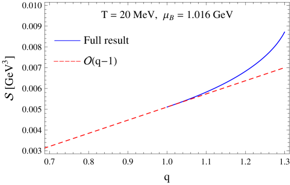
(a)

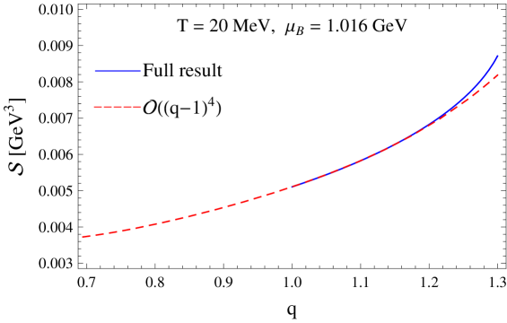
(b)

Figure 1: Entropy density for different $q$ values with a fixed temperature of $T=20$ MeV and a fixed chemical potential $\mu_{B}=1.016$ GeV. The continuous blue line represents the full results and the dashed red lines the expansions up to a) $(q-1)$ and b) $(q-1)^{4}$.

We also display in Fig. 2 the total baryonic density ${\cal N}$, defined in Eq. (20), for different values of $q$ as a function of the particle mass for fixed temperatures and the same chemical potential as in the graphs for the entropy. Up to a certain mass, of the order of 1.05 GeV at $T=20$ MeV and 1.1 GeV at $T=30$ MeV, non extensivity plays almost no role, but as $q$ and $T$ increase, heavier particles are favored. Of course, the value of the chosen chemical potential defines the mass value for which non extensivity becomes important and the chosen chemical potential is of the order of the baryon chemical potencials of the particles in stellar medium that will be investigated in the next sections.

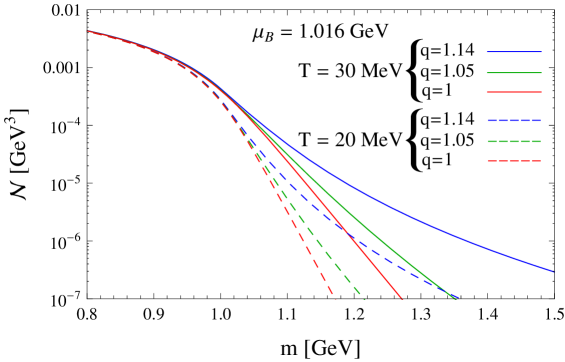
(a)

Figure 2: Baryonic density as a function of baryon mass for different $q$ values, $T=20$ and 30 MeV and $\mu_{B}=1.016$ GeV.

2.3 Stellar matter

In stellar matter there are two conditions that have to be fulfilled, namely, charge neutrality and $\beta$-stability and they read:

$$\sum_{j}q_{j}n_{j}+\sum_{l}q_{l}n_{l}=0,$$ (23)

where $q_{type},type=j,l$ stand for the electric charge of baryons and leptons respectively and

$$\mu_{j}=q_{j}\mu_{n}-q_{e}(\mu_{e}-\mu_{\nu}),\qquad\mu_{\mu}=\mu_{e}.$$ (24)

We have also used the non extensive statistics for the leptons, which enter the calculation as free particles obeying the above mentioned conditions.

The three snapshots of the time evolution of a neutron star in its first minutes of life are given by:

• ${\cal S}/n_{B}=1$, $Y_{l}=0.3$,

• ${\cal S}/n_{B}=2$, $\mu_{\nu}=0$,

• ${\cal S}/n_{B}=0$, $\mu_{\nu}=0$,

where

$$Y_{l}=\frac{\sum_{l}n_{l}}{n_{B}},$$ (25)

which, according to simulations Burrows:1986me , can reach $Y_{l}\simeq 0.3-0.4$. In the present work we are interested in finite temperature systems and hence, most of the results refer to the first two snapshots.

Another aspect of the evolution of compact stars that is worth investigating is the direct Urca (DU) process, $n\to p+e^{-}+\bar{\nu}_{e}$ urca . It is known that the cooling of the star by neutrino emission can occur relatively fast if it is allowed, what happens when the proton fraction exceeds a critical value $x_{\rm\scriptscriptstyle DU}$urca , evaluated in terms of the leptonic fraction as klaen06 :

$$x_{\rm\scriptscriptstyle DU}=\frac{1}{1+(1+x_{e}^{1/3})^{3}}\>,$$ (26)

where $x_{e}=n_{e}/(n_{e}+n_{\mu})$ is the electron leptonic fraction, $n_{e}$ is the number density of electrons and $n_{\mu}$ is the number density of muons. Cooling rates of neutron stars seem to indicate that this fast cooling process does not occur and, therefore, a constraint is set imposing that the direct Urca process is only allowed in stars with a mass larger than $1.5\,M_{\odot}$, or a less restrictive limit, $1.35\,M_{\odot}$ klaen06 . The DU process can also occur for hyperons, if they are taken into account in the EOS. Although the neutrino luminosities in these processes are much smaller than the ones obtained in the nucleon direct Urca process, they play an important role if they occur at densities below the nucleon direct Urca process urca2 . The process $\Lambda\to p+e+\bar{\nu}$, for instance, may occur at densities below the nucleon DU onset. In the next section we also investigate the effects of non extensive statistics on the onset of the DU process.

To make our results depend as little as possible on too many degrees of freedom, we start by analysing the EOS with nucleons only for different values of $q$. We also investigate the effects of non extensivity on a free Fermi gas at finite temperature, where nucleons and leptons are only subject to the conditions of $\beta$-equilibrium and charge neutrality. As it is widely accepted that hyperons should be present inside (proto)neutron stars, they are also included and the effects of using different $q$ values, always larger than one, are checked.

3 Results

We now calculate and analyze stellar properties obtained with two different values of the non extensive statistics $q$ parameter, namely $q=1.05$ and 1.14. Our results are then compared with the ones shown in Ref. lavagno . We have chosen values larger than one because lower values produce a slightly softer EOS, which result in lower maximum stellar masses as compared with the standard non-linear Walecka model, as can be seen in Ref. lavagno and therefore, may not useful if we want to explain massive compact objects. In addition, in Ref. Beck it was shown that there is an upper limit for the entropic index at $q_{max}=11/9$. On the other hand, all experimental information on hadronic systems show that $q>1$. Since our main goal is to check whether 2$M_{\odot}$ stars can be attained with the help of non extensive thermodynamics when the traditional one fails, we restrict ourselves to values that go in the desired direction. In Ref. Lucas , the entropic index $q$, is taken as a fixed property of the hadronic matter with its value determined as $q=1.14$ from the analysis of $p_{T}$-distributions and in the study of the hadronic mass spectrum. The value $q=1.05$ is used because it is slightly larger than the value used in lavagno , where the authors used $q=1.03$ that represents just a small deviation from the standard stellar matter physics. We have checked that the results obtained with $q=1.03$ and $q=1.05$ are numerically very similar. Had we plotted the next figures with both of them, the curves would be practically undistinguishable.

In all graphs shown next, the GM1 parametrization was used, but the qualitative results are the same for the IU-FSU parameter set, despite the inclusion of the $\omega-\rho$ interaction. Another aspect that we should mention is that quantum hadrodynamic models cannot describe the very low density part of the EOS well and they are usually linked to an appropriate EOS named BPS bps at low densities and zero temperature. In the present work we have chosen not to use the BPS, which does not affect the macroscopic quantities we are interested in analyse. Moreover, non extensive thermodynamics is only valid at finite temperature, where the BPS would only be an approximate EOS.

We start by showing the EOS for the first two snapshots of the star evolution in Fig. 3 for the cases with nucleons only and also with hyperons. As it is always the case, hyperons make the EOS softer for a fixed $q$ value. It is difficult to distinghish the curves for our choice of $q$’s because numerically they are indeed very close, but not identical. The deviation obtained with non extensive statistics is very small, but larger at high densities for the $q$-values we have considered, with consequences in the maximum stellar masses, which will be seen later. It is important to observe that, for a fixed $q$-value, the EOS is slightly harder for ${\cal S}/n_{B}=2$, $\mu_{\nu}=0$ than for ${\cal S}/n_{B}=1$, $Y_{l}=0.3$ when only nucleons are taken as internal neutron star constituents, but it is softer when the hyperons are considered. Nevertheless, this behaviour is valid also for the usual thermodynamics, when $q=1$ and hence, it is not a consequence of the use of non extensivity.

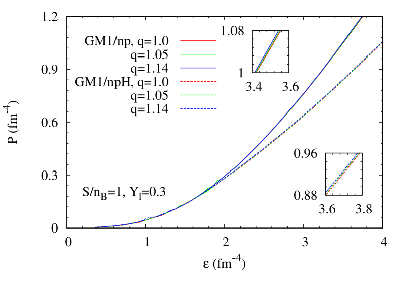
(a)

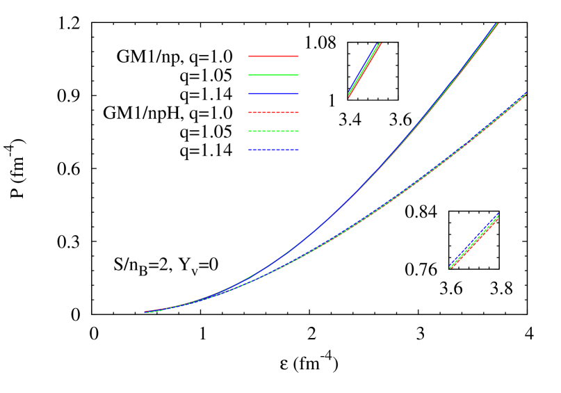
(b)

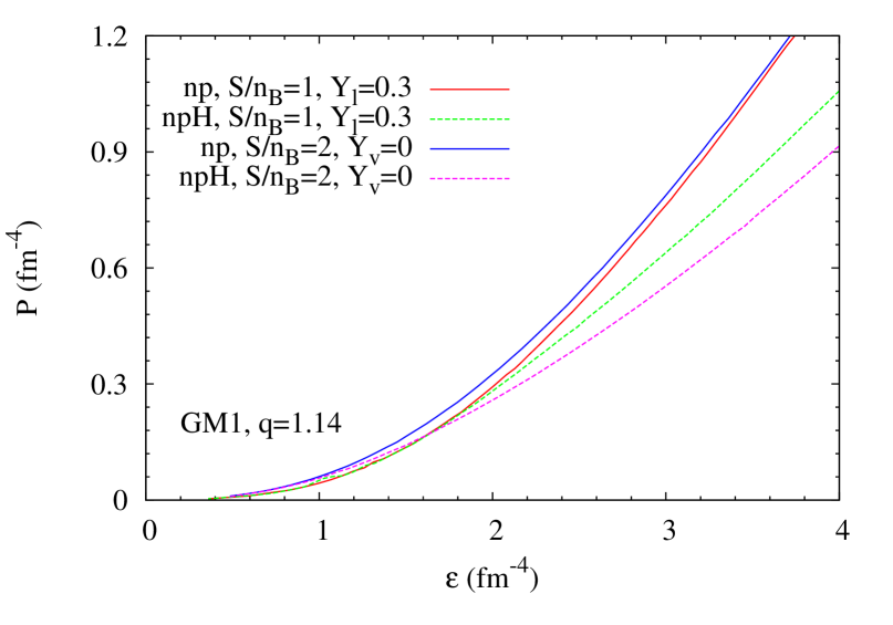
(c)

Figure 3: Equation of state for hadronic matter constituted by nucleons only (np) and including the lightest eight baryons (npH) for different values of $q$ and a) first b) second snapshot of the star evolution c) for $q=1.14$ only and both snapshots.

We then analyze the effects of non extensivity on the internal stellar temperature by plotting the temperature as a function of density again for the first two snapshots of the star evolution in Fig. 4 for both parametrizations investigated in the present work. We display temperature results for densities higher than nuclear matter saturation density because at subsaturation densities, the EOS would be more similar to the one of a free Fermi gas and at very low densities a BPS-like EOS would have to be employed, what we have not done. Nevertheless, we can see from Tables 2 and 3 that the effects of non extensivity on a free gas at fixed temperature are very small, which means that the curves would tend to get closer to each other as the density and the temperature decrease. Then, we clearly see that the temperature decreases with the increase of $q$, a behavior already expected from the calculations performed in ours (see, for instance figs. 2 and 6 of that reference). At densities of the order of 5 times nuclear saturation density, the temperature decreases by approximately 25% in average, with important consequences in the neutrino diffusion during the Kevin-Helmholtz epoch, when the star evolves from a hot and lepton rich object to a cold and deleptonized compact star. The cooling would be faster for larger $q$ values. However, in Ref. lavagno , the behavior is exactly the opposite, i.e. the temperature increases with the increase of the $q$- value, a result that we do not reproduce. We do not believe that the use of a different expression for the partition function, as we have commented in section 2.2 is responsible for this opposite behaviour.

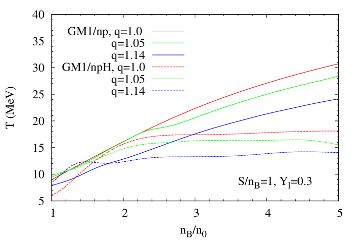
(a)

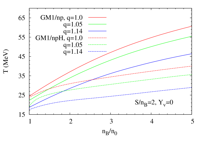
(b)

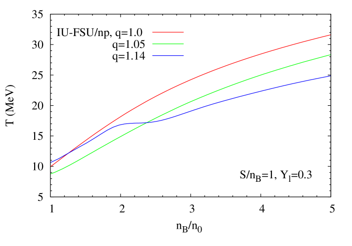
(c)

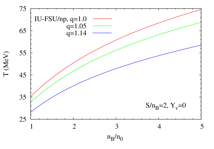
(d)

Figure 4: Temperature as a function of density (in units of nuclear matter saturation density) for different values of $q$ and a) GM1 and first b) GM1 and second c) IU-FSU and first and D) IU-FSU and second snapshot of the star evolution.

In order to see how the internal constitution of the star is affected by non extensivity, we plot in Fig. 5 the particle fractions when the hyperons are considered and the related strangeness content in Fig. 7. We do not include the particle concentrations for the case with nucleons only because, they are affected very little by non extensivity, as shown in Ref. lavagno . From the figures we plot, we can see that as $q$ increases, the amount of strangeness decreases, which means that the EOS becomes harder, resulting in larger maximum masses. On the other hand, we already knew that in a free system, heavier particles are favored when $q$ becomes larger than one, as seen in Fig. 2, a behaviour that is also observed in Fig. 5, i.e., the onset of hyperons takes place at lower densities. But stellar matter is also subject to charge neutrality, $\beta$-equilibrium and different values of temperature at different densities and the final balance results in a system with a slightly smaller strangeness content for larger $q$ values. The numbers used in Fig 7 for the case $S/n_{B}=2$ at $n_{B}/n_{0}\simeq 3$ tell us that as $q$ goes from 1 to 1.05, the decrease in the strangeness content is 2.5%, when it goes from 1.05 to 1.14, it reaches 4.7% and from $q=1$ to $q=1.14$, the decrease is of the order of 7.1%. This decrease makes the EOS harder and hence the explanation for the slightly larger maximum masses obtained with non extensivity.

Neutrinos also play an important role when the lepton fraction is fixed, during the first snapshot of the star evolution. If hyperons are included, neutrinos help in making the EOS harder, but affect very little the EOS if only nucleons are present in the system. This is a well known result for $q=1$. In Fig. 6 we plot only the neutrino fraction, so that its behaviour with $q$ becomes evident. Non extensivity practically does not change the amount of neutrinos. In the difusion approximation normally used in the calculation of the temporal evolution of protoneutron stars in the Kelvin-Helmholtz phase, the neutrino mean free path depends on the diffusion coefficientes, obtained from the EOS and dependent of the neutrino fraction and distribution function. Hence, any change in the neutrino content would certainly influence the stellar evolution, but non extensivity seems not to affect this quantity in a non-neglectable way.

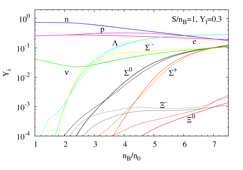
(a)

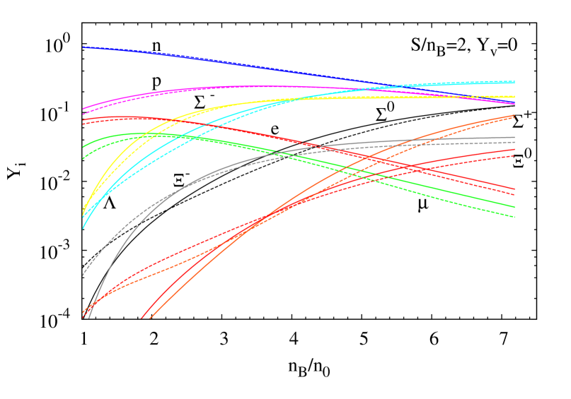
(b)

Figure 5: Particle fractions obtained for a) first and b) second snapshot of the star evolution. We use solid line for $q=1.0$ (standard model) and dashed lines for $q=1.14$.

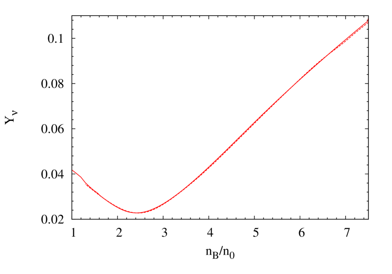
(a)

Figure 6: Neutrino content obtained for the first snapshot of the star evolution. We use solid lines for $q=1.0$ (standard model) and dashed lines for $q=1.14$.

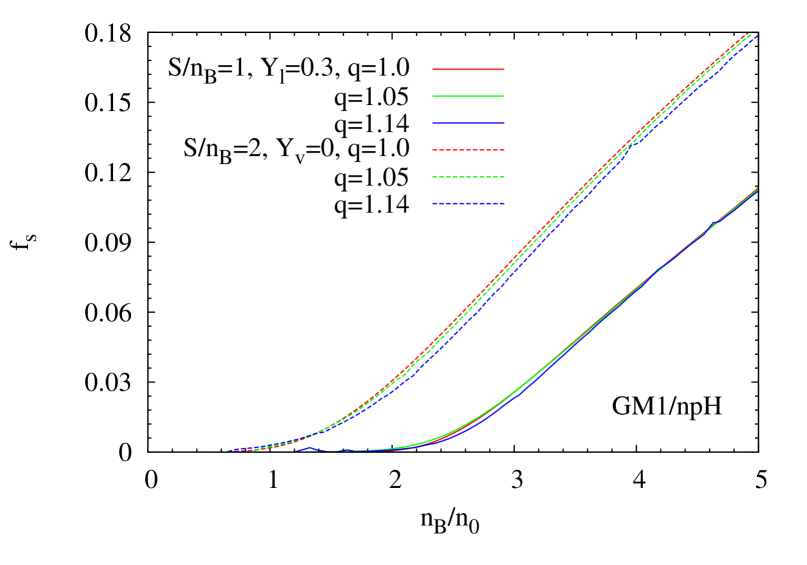
Figure 7: Strangeness content as a function of density (in units of nuclear matter saturation density) for different values of $q$ and two first snapshots of the star evolution.

In Table 2 and Fig. 8 we show the main stellar properties obtained from the solution of the Tolman-Oppenheimer-Volkof (TOV) equations tov , which use the EOS just discussed with the GM1 parametrization as input. As expected, from the observation of the EOS, the maximum stellar mass increases with the increase of the $q$- value. When only nucleons are taken into account, the maximum stellar masses are obtained during the second snapshot of the star evolution (${\cal S}/n_{B}=2$, $\mu_{\nu}=0$) and when hyperons are also included, maximum masses come out for ${\cal S}/n_{B}=1$, $Y_{l}=0.3$. This behavior corroborates the findings in Ref. lavagno . For the sake of completeness, we also display results obtained at fixed temperature ($T=30$ MeV) and compare them with the results for a free Fermi gas, in which case neutrons, protons, electrons and muons obey stellar matter conditions, but are not subject to nuclear interaction. This temperature was chosen to be of interest in the stellar medium, durind the cooling process, as seen in Fig. 7. Of course, we could have chosen $T=20$ MeV instead, a temperature at which chemical freeze-out takes place in heavy ion collisions, but the numerical results would be very similar. In the cases where GM1 was used, there is no obvious pattern with respect to the $q$-value, i.e. the maximum masses oscillate when the $q$-value increases. When a free Fermi gas is used, the maximum masses decrease when $q$ increases. As it is well known the huge increase in the maximum masses is due to the inclusion of the nuclear interaction, but we also found a lack of pattern in a system with fixed temperature instead of fixed entropy. In Fig. 8 we plot mass-radius results obtained from the EOS shown in Fig. 3. In these curves the BPS bps EOS was not included because it is only valid at zero temperature and, as shown in Fig. 4, the temperature at the surface of the star for fixed entropies can be slightly higher. Had we included the BPS EOS, our curves would present a tail towards higher radii, but the differences in the maximum masses would be minor.

To check the consistency of our results, in Table 3 we display, for a system with nucleons only, stellar properties obtained with the IU-FSU parametrization. We have not included hyperons because this parameter sets provides too low maximum stellar masses when strangeness is taken into account. The results show that the qualitative conclusions with respect to the effects of non extensivity do not depend on the chosen parameter set, even when extra crossing terms involving the $\omega-\rho$ interaction is considered.

model	case	$q$	$M_{max}$	$Mb_{max}$	R	${\cal E}_{0}$
			($M_{\odot}$)	($M_{\odot}$)	(Km)	(fm-4)
free gas	T=30 MeV, $Y_{\nu}=0$	1.0	0.693	0.70	7.46	12.59
free gas	T=30 MeV, $Y_{\nu}=0$	1.05	0.689	0.70	7.30	13.48
free gas	T=30 MeV, $Y_{\nu}=0$	1.14	0.680	0.69	7.06	14.32
GM1/np	T=30 MeV, $Y_{\nu}=0$	1.0	2.10	2.37	11.48	5.83
GM1/np	T=30 MeV, $Y_{\nu}=0$	1.05	2.30	2.66	11.34	6.00
GM1/np	T=30 MeV, $Y_{\nu}=0$	1.14	2.29	2.64	11.36	5.85
GM1/np	${\cal S}/n_{B}=1$, $Y_{l}=0.3$	1.0	2.31	2.67	11.57	5.18
GM1/np	${\cal S}/n_{B}=1$, $Y_{l}=0.3$	1.05	2.31	2.67	11.38	5.77
GM1/np	${\cal S}/n_{B}=1$, $Y_{l}=0.3$	1.14	2.32	2.68	11.61	5.18
GM1/np	${\cal S}/n_{B}=2$, $Y_{\nu}=0$	1.0	2.33	2.66	11.60	5.71
GM1/np	${\cal S}/n_{B}=2$, $Y_{\nu}=0$	1.05	2.33	2.68	11.64	5.62
GM1/np	${\cal S}/n_{B}=2$, $Y_{\nu}=0$	1.14	2.34	2.70	11.61	5.71
GM1/np	T=0, $Y_{\nu}=0$	1.0	2.38	2.88	11.75	5.62
GM1/npH	T=30 MeV, $Y_{\nu}=0$	1.0	1.90	2.12	10.88	6.28
GM1/npH	T=30 MeV, $Y_{\nu}=0$	1.05	1.90	2.11	10.73	6.78
GM1/npH	T=30 MeV, $Y_{\nu}=0$	1.14	1.89	2.07	10.61	6.93
GM1/npH	${\cal S}/n_{B}=1$, $Y_{l}=0.3$	1.0	2.10	2.39	11.40	5.69
GM1/npH	${\cal S}/n_{B}=1$, $Y_{l}=0.3$	1.05	2.11	2.54	11.43	5.72
GM1/npH	${\cal S}/n_{B}=1$, $Y_{l}=0.3$	1.14	2.11	2.39	11.44	5.84
GM1/npH	${\cal S}/n_{B}=2$, $Y_{\nu}=0$	1.0	1.93	2.15	10.98	6.46
GM1/npH	${\cal S}/n_{B}=2$, $Y_{\nu}=0$	1.05	1.95	2.18	11.10	6.29
GM1/npH	${\cal S}/n_{B}=2$, $Y_{\nu}=0$	1.14	1.96	2.20	11.13	6.26
GM1/npH	T=0, $Y_{\nu}=0$	1.0	2.00	2.32	11.51	5.96

Table 2: Protoneutron star macroscopic properties (maximum gravitation mass, maximum baryonic mass, corresponding radius and central energy density) for different values of $q$ and fixed temperature or one of the snapshots of the star evolution.

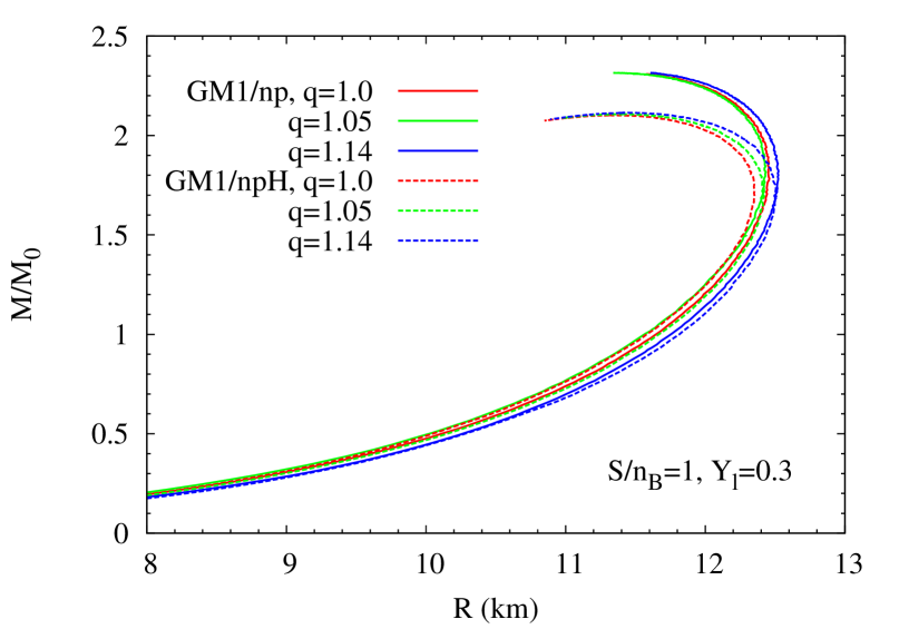
(a)

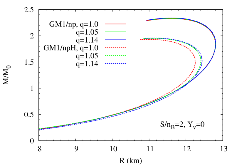
(b)

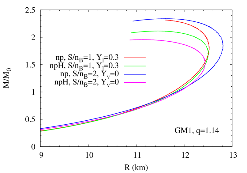
(c)

Figure 8: Mass-radius results obtained from the solution of the TOV equations for hadronic matter constituted by nucleons only (np) and including the lightest eight baryons (npH) for different values of $q$ and a) first b) second snapshot of the star evolution c) for $q=1.14$ only and both snapshots.

model	case	$q$	$M_{max}$	$Mb_{max}$	R	${\cal E}_{0}$
			($M_{\odot}$)	($M_{\odot}$)	(Km)	(fm-4)
free gas	T=30 MeV, $Y_{\nu}=0$	1.0	0.693	0.70	7.46	12.59
free gas	T=30 MeV, $Y_{\nu}=0$	1.05	0.689	0.70	7.30	13.48
free gas	T=30 MeV, $Y_{\nu}=0$	1.14	0.680	0.69	7.06	14.32
IU-FSU/np	T=30 MeV, $Y_{\nu}=0$	1.0	1.90	2.19	10.76	6.08
IU-FSU/np	T=30 MeV, $Y_{\nu}=0$	1.05	1.90	2.19	10.71	6.46
IU-FSU/np	T=30 MeV, $Y_{\nu}=0$	1.14	1.89	2.16	10.57	6.84
IU-FSU/np	${\cal S}/n_{B}=1$, $Y_{l}=0.3$	1.0	1.89	2.13	10.55	6.59
IU-FSU/np	${\cal S}/n_{B}=1$, $Y_{l}=0.3$	1.05	1.94	2.25	11.33	6.34
IU-FSU/np	${\cal S}/n_{B}=1$, $Y_{l}=0.3$	1.14	1.94	2.14	11.30	6.34
IU-FSU/np	${\cal S}/n_{B}=2$, $Y_{\nu}=0$	1.0	1.97	2.19	11.29	5.86
IU-FSU/np	${\cal S}/n_{B}=2$, $Y_{\nu}=0$	1.05	1.97	2.20	11.25	5.96
IU-FSU/np	${\cal S}/n_{B}=2$, $Y_{\nu}=0$	1.14	1.98	2.22	11.24	5.97
IU-FSU/np	T=0, $Y_{\nu}=0$	1.0	1.95	2.28	10.82	6.37
IU-FSU/npH	T=0, $Y_{\nu}=0$	1.0	1.52	1.71	10.31	6.90

Table 3: Same as Table 2

We now analyse the radii results. According to Ref. Hebeler , the radii of the canonical $1.4M_{\odot}$ neutron star should lie in the range 9.7-13.9 Km. Based on an analysis in which it was assumed that all neutron stars have the same radii, they should lie in the range $R=9.1^{+1,3}_{-1.5}$ guillot and another calculation, based on a Bayesian analysis, foresees radii of all neutron stars to lie in between 10 and 13.1 Km Lattimer2013 . The radii results shown in Tables 2 and 3 correspond to the maximum mass stars. If only nucleons are considered as neutron star constituents, as $q$ increases no general pattern is found for the resulting radii. However, when hyperons are taken into account, the radii increase with the increase of $q$. These radii, even for $q=1.14$ are not too large, varying around 11.5 Km. However, if we consider the radii of the canonical 1.4 M_⊙ stars, we can see, from Fig. 8 that non extensivity generally makes them slightly larger and they stand around 12 Km, a somewhat large value if the above mentioned constraints are to be taken seriously. Had we included the BPS EOS, they would be still a bit larger. Let’s stress that the radii are determined by the parametrization chosen, depending also on the hyperon-meson coupling constants. Hence, if a model succeeds in describing a small radius, non extensivity is not likely to modify it too much.

Finally, in Fig. 9 we plot the onset of the direct Urca process in stellar matter for matter with (dashed lines) and without hyperons (solid lines) in the case where ${\cal S}/n_{B}=2$, $\mu_{\nu}=0$. The lines around a y-value of 0.12 refer to $x_{DU}$ and the other lines represent the proton fraction. When the curves cross, we can see the value of the proton fraction and the respective baryonic density. We can see that the line for $x_{DU}$ coincides for the standard model independently of considering or not hyperons. For $q=1.14$ both curves present a small deviation at large densities. For GM1, the standard density value for which the DU process occurs (at zero temperature and matter without hyperons) is 1.81 times nuclear matter saturation density rafael11 . When we fix the entropy density to 2 and keep $q=1$, this value decreases to 1.207 (1.205) $n_{B}/n_{0}$ with (without) hyperons but when we look at the values for $q=1.14$, we see that the onset of the DU process increases again by approximately 21.5% to 1.423 (1.402) $n_{B}/n_{0}$ with (without) hyperons. The proton fraction that we obtain with nucleons only and with hyperons are coincident for a fixed $q$-value at low densities and just deviate from each other when other hyperons with positive charge appear. Therefore, if the DU process determines how the star cools down, a system described by non extensive statistics would certainly affect the interpretation of the cooling rate mechanism.

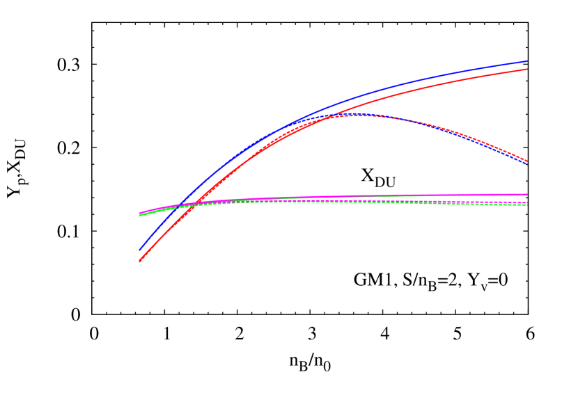
(a)

Figure 9: Onset of direct Urca process in stellar matter with nucleons only (solid lines) and with hyperons (dashed lines) for the usual Boltzmann-Gibbs statistics (q=1, blue and pink lines) and for $q=1.14$ (red and green lines).

4 Final Remarks

We have applied non extensive statistics to calculate equations of state that describe stellar matter with two of the commonly used parametrizations for the non-linear Walecka model, namely GM1 gm1 and IU-FSU iufsu . We have then fixed two $q$-values (1.05 and 1.14) and obtained the most important microscopic quantities associated with the equations of state, i.e. particle fractions, strangeness, internal temperature and direct Urca process onset for two snapshots of the star evolution. As compared with the existing work on the application of non extensive thermodynamics lavagno , some new features were investigated, apart from the use of two different parameter sets. We have confirmed that the equations of state are only slightly modified, but the effects are enough to produce stars with slightly higher maximum masses and these results are common to both parameter sets used. However, contrary to what was obtained in lavagno , we found that the internal temperature of the stars decreases with the increase of the $q$-value and at densities of the order of 5 times nuclear saturation density, the temperature decreases by approximately 25% in average, with important consequences in the neutrino diffusion during the Kevin-Helmholtz epoch, when the star evolves from a hot and lepton rich object to a cold and deleptonized compact star. This aspect should certainly be better investigated. Moreover, we have also seen that the direct Urca process is substantially affected by non extensivity, with consequences on the cooling rates of the stars.

As usually done in the search for macroscopic star properties, the Tolman-Oppenheimer-Volkof equations were then solved for the previously obtained EOS and the macroscopic quantities were computed. The results were compared with more academic calculations for fixed temperatures and for a free-Fermi gas but in these cases, due to the imposition of stellar matter constraints, no specific pattern was found, differently from what happens in a system with really free gases, as seen in Figs. 1, 2 and in Ref. ours .

A final word on our choice of $q$ values larger than one is worthy. All experimental information on hadronic systems show that $q>1$ and according to Ref. Beck , there is an upper limit for the entropic index at $q_{max}=11/9$. We have checked that it is possible to use the sub-extensive regime with the help of an appropriate expansion, but it does not make sense in applications to protoneutron stars if the desired effect is to increase the maximum mass and this regime makes it decrease.

In this work, we have also used the non extensive statistics for the leptons, which enter the calculation as free particles with respect to the strong nuclear interaction, but subject to the conditions of charge neutrality and $\beta$-equilibrium. We could have used different $q$-values for the leptons, but for simplicity, we have opted to use the same values as for the baryons.

- (1) J. M. Lattimer and M. Prakash, Science 304, 536 (2004).
- (2) W. Keil and H. Janka, Astron. Astrophys. 296, 145 (1995).
- (3) J. A. Pons, S. Reddy, M. Prakash, J. M. Lattimer and J.A. Miralles, Astrophys. J. 513, 780 (1999); J. A. Pons, A. W. Steiner, M. Prakash and J. M. Lattimer, Phys. Rev. Lett. 86 (2001) 5223-5226.
- (4) M. Prakash, I. Bombaci, M. Prakash, P. J. Ellis, J. M. Lattimer and R. Knorren, Phys. Rept. 280, 1 (1997).
- (5) B.D. Serot and J.D. Walecka, Adv. Nucl. Phys. 16 (1986) 1.; J. Boguta and A. R. Bodmer, Nucl. Phys. A 292, 413 (1977).
- (6) N. K. Glendenning, Compact Stars, Springer-Verlag, New-York, 2000.
- (7) P. Haensel, A. Y. Potekhin, D. G. Yakovlev: Neutron Stars, Equation of State and Structure, Springer, New York (2006).
- (8) Paul Demorest, Tim Pennucci, Scott Ransom, Mallory Roberts, and Jason Hessels, Nature (London) 467, 1081 (2010).
- (9) J. Antoniadis et al, Science 26, 340 n. 6131 (2013).
- (10) C. Tsallis, J. Stat. Phys. 52 (1988) 479.
- (11) M. Gell-Mann, C. Tsallis, Nonextensive Entropy: Interdisciplinary Applications, Oxfor University Press, USA, 2004.
- (12) I. Bediaga, E.M.F. Curado e J.M. de Miranda, Physica A 286 (2000) 156.
- (13) A. Deppman, Physica A 391 (2012) 6380; Physica A 400 (2014) 207.
- (14) A. Lavagno and D. Pigato, Eur. Phys. J. A (2011) 47: 52.
- (15) C. Beck, Physica A 286, 164 (2000).
- (16) J. Cleymans e D. Worku, J. Phys. G: Nucl. Part. Phys. 39 (2012) 025006.
- (17) R. Hagedorn, Lect. Notes Phys. 221, 53 (1985).
- (18) L. Marques, E. Andrade-II and A. Deppman, Phys. Rev. D 87, 114022 (2013).
- (19) L. Marques, J. Cleymans and A. Deppman, Phys. Rev. D 91, 054025 (2015).
- (20) I. Sena and A. Deppman, Eur. Phys. J. A 49 (2013) 17.
- (21) A. Deppman, J. Phys. G 41, 055108 (2014).
- (22) Eugenio Megías, Débora P. Menezes and Airton Deppman, Physica A: Statistical Mechanics and its Applications 421, 15-24 (2015).
- (23) E. Megías, D. P. Menezes and A. Deppman, EPJ Web Conf. 80, 00040 (2014).
- (24) A. Deppman, E. Megías and D. Menezes, J. Phys. Conf. Ser. 607, no. 1, 012007 (2015).
- (25) M. Dutra, O. Lourenço, S. S. Avancini, B. v. Carlson, A. Delfino, D. P. Menezes, C. Providencia, S. Typel and J. R. Stone, Phys. Rev. C 90, 055203 (2014).
- (26) N. K. Glendenning and S. A. Moszkowski, Phys. Rev. Lett. 67, 2414 (1991)
- (27) F. J. Fattoyev, C. J. Horowitz, J. Piekarewicz and G. Shen, Phys. Rev. C 82, 055803 (2010); (arxiv:1008.3030).
- (28) C. J. Horowitz and J. Piekarewicz, Phys. Rev. Lett. 86, 5647 (2001).
- (29) B. G. Todd-Rutel and J. Piekarewicz, Phys. Rev. Lett. 95, 122501 (2005); F. J. Fattoyev and J. Piekarewicz, Phys. Rev. C 82, 025805 (2010).
- (30) Constança Providência, Sidney S. Avancini, Rafael Cavagnoli, Silvia Chiacchiera, Camille Ducoin, Fabrizio Grill, Jerome Margueron, Débora P. Menezes, Aziz Rabhi, Isaac Vidaña, Eur. Phys. J. A (2014) 50:44.
- (31) J. Schaffner-Bielich, A. Gal, Phys. Rev. C 62, 034311 (2000); J. Schaffner-Bielich, M. Hanauske, H. Stocker and W. Greiner, Phys. Rev. Lett. 89, 171101 (2002); E. Friedman, A. Gal, Phys. Rep. 452, 89 (2007).
- (32) Luiz L. Lopes and Debora P. Menezes, Phys. Rev. C 89, 025805 (2014).
- (33) J. M. Conroy, H. G. Miller and A. R. Plastino, Physics Letters A 374 (2010) 4581–4584.
- (34) J. Rozynek, Physica A 440, 27 (2015).
- (35) T. S Biró, K. M Shen and B. W Zhang, Physica A 428, 410 (2015).
- (36) A. Burrows and J. M. Lattimer, Astrophys. J. 307, 178 (1986).
- (37) J. M. Lattimer, C. J. Pethick, M. Prakash, and P. Haensel, Phys. Rev. Lett. 66, 2701 (1991).
- (38) T. Klähn, et al., Phys. Rev. C 74, 035802 (2006).
- (39) M. Prakash, J. M. Lattimer, and C. J. Pethick, Astrophys. J. 390, L77 (1992).
- (40) G. Baym, C. Pethick, and D. Sutherland, Astrophys. J. 170, 299 (1971).
- (41) R. C. Tolman, Phys. Rev. 55, 364 (1939); J. R. Oppenheimer and G. M. Volkoff, Phys. Rev. 55, 374 (1939).
- (42) K. Hebeler, J. M. Lattimer, C. J. Pethick and A. Schwenk, Phys. Rev. Lett. 105 (2010) 161102.
- (43) S. Guillot, M. Servillat, N. A. Webb and R. E. Rutledge, ApJ 772 (2013) 7.
- (44) J. M. Lattimer and A. W. Steiner, Astrophys. J. 784, 123 (2014).
- (45) Rafael Cavagnoli, Constança Providência, and Debora P. Menezes, Phys. Rev. C 83, 045201 (2011).