HACC: Simulating Sky Surveys on State-of-the-Art Supercomputing Architectures

Abstract

Current and future surveys of large-scale cosmic structure are associated with a massive and complex datastream to study, characterize, and ultimately understand the physics behind the two major components of the ‘Dark Universe’, dark energy and dark matter. In addition, the surveys also probe primordial perturbations and carry out fundamental measurements, such as determining the sum of neutrino masses. Large-scale simulations of structure formation in the Universe play a critical role in the interpretation of the data and extraction of the physics of interest. Just as survey instruments continue to grow in size and complexity, so do the supercomputers that enable these simulations. Here we report on HACC (Hardware/Hybrid Accelerated Cosmology Code), a recently developed and evolving cosmology N-body code framework, designed to run efficiently on diverse computing architectures and to scale to millions of cores and beyond. HACC can run on all current supercomputer architectures and supports a variety of programming models and algorithms. It has been demonstrated at scale on Cell- and GPU-accelerated systems, standard multi-core node clusters, and Blue Gene systems. HACC’s design allows for ease of portability, and at the same time, high levels of sustained performance on the fastest supercomputers available. We present a description of the design philosophy of HACC, the underlying algorithms and code structure, and outline implementation details for several specific architectures. We show selected accuracy and performance results from some of the largest high resolution cosmological simulations so far performed, including benchmarks evolving more than 3.6 trillion particles.

1 Introduction

1.1 Sky Surveys and Computational Cosmology

An unprecedented volume of observational data and information regarding the distribution and properties of optical sources in the Universe is becoming available from ongoing and future sky surveys, both imaging and spectroscopic. These include BOSS (Baryon Oscillation Spectroscopic Survey; Dawson et al. 19), DES (Dark Energy Survey; Abbott et al. 3), KiDS (Kilo-Degree Survey; de Jong et al. 21), SUMIRE, DESI (Dark Energy Spectroscopic Instrument; Levi et al. 49), 4MOST (4-meter Multi-Object Spectroscopic Telescope; de Jong et al. 22), J-PAS (Javalambre-Physics of the Accelerated Universe Astrophysical Survey; Benitez et al. 8), LSST (Large Synoptic Survey Telescope; Abell et al. 1), Euclid [4], and WFIRST (Wide-Field InfraRed Survey Telescope; Spergel et al. 62). Combined with microwave background observations from the Planck satellite and ground-based telescopes, such as ACT (Atacama Cosmology Telescope) and SPT (South Pole Telescope), the mining of these and other datasets, such as resulting from new radio surveys, e.g., VLASS (Very Large Array Sky Survey) and X-ray surveys, are expected to yield a host of cosmological and astrophysical insights.

There are several foundational cosmological questions that the datasets will directly address. Perhaps the most pressing is the mysterious cause of the accelerated expansion of the Universe – whether it is due to dark energy or a modification of general relativity. In addition, the observations will also bear on the ultimate nature of dark matter, provide information on the physics of the early Universe by probing primordial fluctuations, and enhance our knowledge of the neutrino family, the lightest known massive particles in the Universe. Aside from these basic cosmological questions, the survey data provides an enormous resource for attacking a very large number of astrophysical problems related primarily to understanding the formation of complex structure in the Universe.

In order to extract the full extent of information from these remarkable surveys, a similar level of effort must be undertaken in the realm of theory and modeling. To attain the necessary realism and accuracy, sophisticated, large scale simulations of structure formation must be carried out. These simulations address a large variety of tasks: providing predictions for many different cosmological models to solve the inverse problem related to determining cosmological parameters, investigating astrophysical and observational systematics that could mimic physics effects of the dark sector, enabling careful calibration of errors (by providing precision covariance estimates), testing, optimizing, and validating observational strategies with synthetic catalogs, and finally, exploring new and exciting ideas that could either explain puzzling aspects of the observations (such as cosmic acceleration) or help to motivate and design the implementation of new types of cosmological probes.

The simulations have to be large enough in volume to cover the observed Universe (or at least a large part of it) and at the same time possess sufficient mass and force resolution (a spatial dynamic range of roughly a million) to resolve objects down to the smallest relevant scales. As one example, a recently constructed synthetic galaxy and quasar catalog for DESI is shown in Figure 1. This catalog was based on a 1.1 trillion-particle HACC simulation, with a box-size of $\sim 4$ Gpc (White et al. 75).

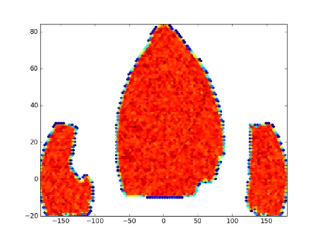
Figure 1: Areal density of emission line galaxies from synthetic catalogs produced for the DESI experiment (White et al. 75). These catalogs are based on results from a high resolution, trillion particle HACC simulation performed on the Mira supercomputer. They are being used to test fiber assignment algorithms and to optimize DESI’s footprint and survey strategy.

The diverse uses of simulations outlined above also demand fast turn-around times, as not one such simulation is required but, eventually, many hundreds to hundreds of thousands. The simulation codes, therefore, have to be capable of exploiting the largest supercomputing platforms available today and into the future.

1.2 Challenge of Future Supercomputing Architectures

Viewed as a single entity, the field of ‘modern’ computational cosmology (Klypin & Shandarin 45, Efstathiou et al. 27) has largely kept pace with the growth of computational power, but new challenges will need to be faced over the next decade. This is due to the failure of Dennard scaling (Dennard et al. 24), which underlay the success of Moore’s Law for about two decades. As a consequence of the fact that single-core clock rate and performance have stalled since 2004/5, the design of future microprocessors is branching into several new directions, to overcome the related performance bottlenecks (Borkar & Chien 13) – the key constraint being set by electrical power requirements. The resulting impact on large supercomputers is already being seen; aside from the familiar large multi-core processor clusters, two major approaches can be easily identified.

The first approach is the large homogeneous system, built around a ‘system on chip’ (SoC) design or around many-core nodes, with concurrencies in the multi-million range – the IBM Blue Gene/Q is an excellent example of such an approach; specific examples include Sequoia (20 PFlops peak) at Lawrence Livermore National Laboratory and Mira (10 PFlops peak) at Argonne National Laboratory, supporting up to $6.3$ million-way concurrency (Sequoia; half of that on Mira). The second route is to take a conventional cluster but to attach computational accelerators to the CPU nodes. The accelerators can range from the IBM Cell processor (as on Los Alamos National Laboratory’s Roadrunner, first to break the Petaflop barrier), to GPUs as on Titan (27 PFlops peak) at Oak Ridge National Laboratory, to the Intel Xeon Phi coprocessor as on Stampede (10 PFlops peak) at the Texas Advanced Computing Center. Future evolution of supercomputer systems will almost certainly involve further branching in the space of possible architectures.

Because development of the supercomputing software environment is likely to lag significantly behind the pace of hardware evolution, it appears prudent, if not essential, to develop a code design philosophy and implementation plan for cosmological simulations that can be reconfigured relatively quickly for new architectures, has support for multiple programming paradigms, and at the same time, can extract high levels of sustained performance. With this challenge in mind, we have designed HACC (Hardware/Hybrid Accelerated Cosmology Codes), an N-body cosmology code framework that takes full advantage of all available architectures. This paper presents an overview of HACC ‘theory and practice’ by covering the methods employed, as well as describing important components of the implementation strategy. An example of HACC’s capabilities is shown in Figure 2, a recent large cosmological run on Mira, evolving more than 1 trillion particles; this is the same simulation on which the results of Figure 1 are based.

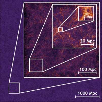
Figure 2: Zoom-in visualization of the density field in a 1.07 trillion particle, $4.225~{}\hbox{Gpc}$ box-size simulation with HACC on 32 Blue Gene/Q racks. The force resolution is $6$ kpc and the particle mass, $m_{p}\sim 2.6\cdot 10^{9}$ M_⊙. The image, taken during a late stage of the evolution, illustrates the global spatial dynamic range covered by the simulation, $\sim 10^{6}$, although the finer details are not resolved in this visualization.

1.3 HACC Design Motivations and Implementation

Cosmological simulations can be broadly divided into two classes: gravity-only N-body simulations and ‘hydrodynamic’ simulations that incorporate gasdynamics and models of astrophysical processes. Since gravity dominates at large scales, and dark matter outweighs baryons by roughly a factor of five, N-body simulations are an essential component in modeling the formation of structure. Several post-processing strategies can be used to incorporate missing physics in gravity-only codes, such as the halo occupation distribution (HOD) approach (Kauffmann et al. 44; Jing et al. 42; Benson et al. 9; Peacock & Smith 54; Seljak 60; Berlind & Weinberg 12; Zheng et al. 77), Subhalo/Halo Abundance Matching (S/HAM) (Vale & Ostriker 69; Conroy et al. 18; Wetzel & White 72; Moster et al. 51; Guo et al. 30) or semi-analytic modeling (SAM) (White & Frenk 73; Kauffmann et al. 43; Cole et al. 17; Somerville & Primack 61; Benson et al. 10; Baugh 6; Benson 11) for adding galaxies to the simulations. Whenever a more detailed understanding of the dynamics of baryons is required, gasdynamic, thermal, and radiative processes (among others) must be modeled, as well as processes such as star formation and local feedback mechanisms (outflows, AGN/Sn feedback). A compact review of cosmological simulation techniques and applications can be found in [25]. A concise review of phenomenological galaxy modeling is given in [7].

Carrying out a fully realistic first principles simulation program for all aspects of modeling cosmological surveys will not be possible for quite some time. The required gasdynamic simulations are very expensive and there is considerable uncertainty in the modeling and physics inputs. Progress is nevertheless possible by combining high-resolution, large-volume N-body simulations and post-processing inputs from simulations that include gas physics to build robust phenomenological models. The parameters of these models would be determined by a set of observational constraints; yet other observations would then function as validation tests. The HACC approach assumes this starting point as an initial design constraint, but one that can be relaxed in the future.

The overall structure of HACC is based on the realization that a large-scale computational framework must not only meet the challenges of spatial dynamic range, mass resolution, accuracy, and throughput, but, as already discussed, be cognizant of disruptive changes in computational architectures. As an early validation of its design philosophy, HACC was among the pioneering applications proven on the heterogeneous architecture of Roadrunner (Habib et al. 32, Pope et al. 56), the first computer to break the petaflop barrier. With its multi-algorithmic structure, HACC allows the coupling of MPI with a variety of local programming models – MPI+‘X’ – to readily adapt to different platforms. Currently, HACC is implemented on conventional and Cell/GPU-accelerated clusters, on the Blue Gene/Q architecture (Habib et al. 33), and has been run on prototype Intel Xeon Phi hardware. HACC is the first, and currently the only large-scale cosmology code suite world-wide, that has been demonstrated to run at full scale on all available supercomputer architectures.

Another key aspect of the HACC code suite is an inbuilt capability for fast “on the fly” or in situ data analysis. Because the raw data from each run can easily be at the petabyte (PB) scale or larger, it is essential that data compression and data analysis be maximized to the extent possible, before the code output is dumped to the file system. In order to comply with storage and data transfer bandwidth limitations, the amount of data reduction required is roughly two orders of magnitude. HACC’s in situ data analysis system is designed to incorporate a number of parallel tools such as tools for generating clustering statistics (power spectra, correlation functions), tessellation-based density estimators, a fast halo finder [76] with an associated merger tree capability, real-time visualization, etc.

The HACC framework has been used to generate a number of large simulations to carry out a variety of scientific projects. These include a suite of 64 billion particle runs for predicting the baryon acoustic oscillation signal in the quasar Ly-$\alpha$ forest, as observed by BOSS (White et al. 74), a high-statistics study of galaxy group and cluster profiles, to better establish the halo concentration-mass relation (Bhattacharya et al. 15), tests of a new matter power spectrum emulator (Heitmann et al. 38), and a study of the effect of neutrino mass and dynamical dark energy on the matter power spectrum (Upadhye et al. 68). Results from other simulation runs will be available shortly. These range from simulation campaigns in the $\sim 70$ billion particle range per simulation, e.g., simulations for determining sampling covariance for BOSS (Sunayama et al. 65), to individual simulations in the $\sim 500-1000$ billion particle class. As an example of the latter, a recently completed simulation on Titan used 550 billion particles to evolve a 1.3 Gpc periodic box, with mass resolution, $m_{p}=1.48\cdot 10^{8}$ M_⊙, and force smoothing scale of $\sim 3.2$ kpc (Heitmann et al. 39).

The paper is organized as follows. In Section 2 we introduce the basic HACC design and algorithms, focusing on how portability and scaling on very large supercomputers is achieved, including discussions of practical matters such as memory management and parallel I/O. A significant aspect of supercomputer architecture is diversity at the level of the computational nodes. As mentioned above, the HACC design adopts different short-range solvers for different nodal architectures, and this feature is discussed separately in Section 3. Section 4 presents some results from our extensive code verification program, showcasing a comparison test with Gadget-2 [63], one of the most widely used cosmology codes today. The in situ analysis tool suite is covered in Section 5, and selected performance results are given in Section 6. We conclude in Section 7 with a recap and a discussion of future evolution paths for HACC.

2 General Features of the HACC Code Framework

2.1 N-body Algorithms

In the standard model of cosmology, structure formation at large scales is described by the gravitational Vlasov-Poisson equation (Peebles 52), a 6-D partial differential equation for the Liouville flow (1) of the one-particle phase space distribution, arising from the non-relativistic limit of the Vlasov-Einstein set of equations,

$$\partial_{t}f({\mathbf{x}},{\mathbf{p}})+\dot{\mathbf{x}}\cdot\partial_{\mathbf{x}}f({\mathbf{x}},{\mathbf{p}})-\nabla\phi\cdot\partial_{\mathbf{p}}f({\mathbf{x}},{\mathbf{p}})=0,$$ (1)

where the Poisson equation encodes the self-consistency of the evolution:

$$\nabla^{2}\phi({\mathbf{x}})=4\pi Ga^{2}(t)\Omega_{m}\delta_{m}({\mathbf{x}})\rho_{c}.$$ (2)

The expansion history of the Universe is given by the time-dependence of the scale factor $a(t)$ governed by the specifics of the cosmological model, the Hubble parameter, $H=\dot{a}/a$, $G$ is Newton’s constant, $\rho_{c}$ is the critical density, $\Omega_{m}$, the average mass density as a fraction of $\rho_{c}$, $\rho_{m}({\mathbf{x}})$ is the local mass density, and $\delta_{m}({\mathbf{x}})$ is the dimensionless density contrast,

$$\rho_{c}=3H^{2}/8\pi G,~{}~{}~{}\delta_{m}({\mathbf{x}})=(\rho_{m}({\mathbf{x}})-\langle\rho_{m}\rangle)/\langle\rho_{m}\rangle,$$ (3)

$${\mathbf{p}}=a^{2}(t)\dot{\mathbf{x}},~{}~{}~{}\rho_{m}({\mathbf{x}})=a(t)^{-3}m\int d^{3}{\mathbf{p}}f({\mathbf{x}},{\mathbf{p}}).$$ (4)

In general, the Vlasov-Poisson equation is computationally very difficult to solve as a partial differential equation because of its high dimensionality and the development of nonlinear structure – including complex multistreaming – on ever finer scales, driven by the gravitational Jeans instability. Consequently, N-body methods, using tracer particles to sample $f({\mathbf{x}},{\mathbf{p}})$ are used; the particles follow Newton’s equations, with the forces given by the gradient of the scalar potential $\phi(\mathbf{x})$ (Cf. Braun & Hepp 16; for an early comparison of direct and particle methods in a non-gravitational context, see Denavit & Kruer 23).

The cosmological N-body problem is characterized by a very large value of the number of interacting particles and a very large spatial dynamic range. If one wishes to track billions of galaxy-hosting halos at a reasonable mass resolution, then hundreds of billions to trillions of tracer particles are required. Since gravity cannot be shielded, this obviously precludes the use of brute-force direct particle-particle algorithms for the particle force computation. Popular alternatives include pure particle-based methods (tree codes) or multi-scale grid-based methods (AMR codes), or hybrids of the two (TreePM, particle-particle particle-mesh, P³M). It is not our purpose here to go into many details of the algorithms and their implementations; good coverage of the background material can be found in [5], [41], [71], [53], [26], [63], and [25].

The HACC design approach acknowledges that, as a general rule, particle and grid-based methods both have their limitations. For physics, algorithmic, and data structure reasons, grid-based techniques are better suited to larger (‘smooth’) lengthscales, with particle methods possessing the opposite property. This suggests that higher levels of code organization should be grid-based, interacting with particle information at a lower level of the computational hierarchy.

Following this central idea, HACC uses a hybrid parallel algorithmic structure, splitting the gravitational force calculation into a specially designed grid-based long/medium range spectral particle-mesh (PM) component that is retained on all computational architectures, and an architecture-tunable particle-based short/close-range solver. The spectral PM component can be viewed as an upper layer that is implemented using C++/C/MPI, essentially independent of the target architecture, whereas, the bottom or node level is where the short/close-range solvers reside. These are chosen and optimized depending on the target architecture and use different local programming models as appropriate. Of the 6 orders of magnitude required for the spatial dynamic range for the force solver, the grid is responsible for 4 orders of magnitude, while the particle methods handle the critical 2 orders of magnitude at the shortest scales where particle clustering is maximal and the bulk of the time-stepping computation takes place.

The short-range solvers can employ direct particle-particle interactions, i.e., a P³M algorithm [41], as on some accelerated systems, or use both tree and particle-particle methods as on the IBM Blue Gene/Q (‘PPTreePM’ with a recursive coordinate bisection (RCB) tree). As two extreme cases, in non-accelerated systems, the tree solver provides very good performance but has some complexity in the data structure, whereas for accelerated systems, the local $N^{2}$ approach is more compute-intensive but has a very simple data structure, better-suited for computational accelerators such as Cells and GPUs. The availability of multiple algorithms within the HACC framework also allows us to carry out careful error analyses, for example, the P³M and the PPTreePM versions agree to within $0.1\%$ for the nonlinear power spectrum test in the code comparison suite of  [35] (see Section 4 for more details). This level of error control easily meets the minimal requirements set by the increased statistical power of next-generation survey observations.

In the following we first describe the long/medium-range force solver employed by HACC. As mentioned above, this solver remains unchanged across all architectures. After doing this, we provide details of the architecture-specific short-range solvers, and the sub-cycled time-stepping scheme used by the code suite.

2.2 Particle Overloading

An important aspect of large-volume cosmological simulations is that the density distribution is very highly clustered, with an overall topology descriptively referred to as the “cosmic web”. The clustering is such that the maximum distance moved by a particle is roughly 30 Mpc, very much smaller than the overall scale of the simulation box ($\sim$Gpc). With a 3-D domain decomposition, each (non-cubic) nodal volume (MPI rank) is roughly of linear size 50-500 Mpc, depending on the simulation run size. The idea behind particle overloading is to ‘overload’ the node with particles belonging also to a zone of size roughly 3-10 Mpc extending out from the nominal spatial boundary for that node (so-called “passive” particles). Note that copies of these particles – essentially a replicated particle cache, roughly analogous to ghost zones in PDE solvers – will also be held by other processors, in only one of which will they be “active”, hence the use of the term ‘overloading’. Because more than one copy of these particles is held by neighboring domains, overloading is not the same as the guard zone conventionally used to reduce communication in particle codes.

The point of having this particle cache is two-fold. First, for a number of time steps no particle communication across nodes is required. Additionally, the cached particle ‘skin’ allows particle deposition and force interpolation for the spectral particle-mesh method to be done using information entirely local to a node, thus grid communication is also reduced. The particle cache is refreshed (replacement of passive particles in each computational domain by active particles from neighboring domains) at some given number of time steps. This involves only nearest neighbor communication and the penalty is a trivial fraction of the time spent in a single global time step. The second advantage of overloading is that when a short-range solver is added to each computational domain, no communication infrastructure is associated with this step. Thus, in principle, short-range solvers can be developed completely independently at the node level, and then inserted into the code as desired. Consequently, HACC’s weak scaling is purely a function of the properties of the long-range solver.

The overloaded PM solver is formally exact – each node sends its local density field (computed with active particles only) to the global spectral Poisson solver, which then returns the force for both active and passive particles to each node. The short-range force calculation for passive particles is computed in the same way as for the active particles, except that passive particles, which are closer to the outer domain boundary than the short-range force-matching scale, $r_{s}$ (defined in the following Section), do not have their short-range forces computed, and are subject to only long-range forces. This avoids force anisotropy near the overloaded zone boundary, at the expense of a force error on the passive particles that are close to the edge of the boundary. Since the role of the passive particles is primarily to provide a buffer ‘boundary condition’ zone for the active particles near the nodal domain’s active zone boundary, consequences of this error are easy to control.

Overloading has two associated costs: (i) loss of memory efficiency because of the overloading zone, and (ii) the just-discussed numerical error for the short-range force that slowly leaks in from the edge of the outer (passive particle) domain boundary. In cosmology applications, the memory inefficiency can be tolerated to the point where the memory in passive and active particles is roughly equal, but this is not a limitation in the majority of the cases of interest. The second problem is easily mitigated by balancing the boundary thickness against the frequency of the particle cache refresh, “recycling” the passive particles after some finite number of time-steps, chosen to be such that the refresh time is smaller than the error diffusion time: each domain gets rid of all of its passive particles and then refreshes the passive zone with (high accuracy) active particles exchanged from nearest-neighbor domains.

2.3 The Long-Range Force

Conventional particle-based codes employ a combination of spatial and spectral techniques. The Cloud-in-Cell (CIC) scheme used for particle deposition is an example of a real space operation, whereas the Fast Fourier Transform (FFT)-based Poisson solver is a $k$-space or spectral operation. The spatial operations in a typical particle code are the particle deposition, the force interpolation, and the finite-differences for computing field derivatives. The spectral operations include the influence (or pseudo-Green) function FFT solve, digital filtering, and spectral differentiation techniques. Spatial techniques are often less flexible and more tedious to implement than their spectral counterparts. Also, higher-order spatial operations can be complicated and lead to messy and dense communication patterns (e.g., indirection).

Accurate P³M codes are usually run with Triangle-Shaped-Cloud (TSC), a high-order spatial deposition/filtering scheme, as well as with high-order spatial differencing templates. In terms of grid units, the CIC deposition kernel filters roughly at the level of two grid cells or less with a large amount of associated “anisotropy noise”; TSC filters at about three grid cells with much reduced noise. The resulting long-range/short-range force matching is usually done at four/five grid cells or so (but can be as small as three grid cells). TreePM codes can move the matching point to a larger number of grid cells because of the inherent speed of the tree algorithm, so they can continue to use CIC deposition (with some additional Gaussian filtering). HACC allows the use of both P³M and TreePM algorithms, using a shorter matching scale than most TreePM codes. One advantage of the shorter matching scale is that a low-order polynomial expression can be used in the force representation, which greatly speeds up evaluation of the force kernel.

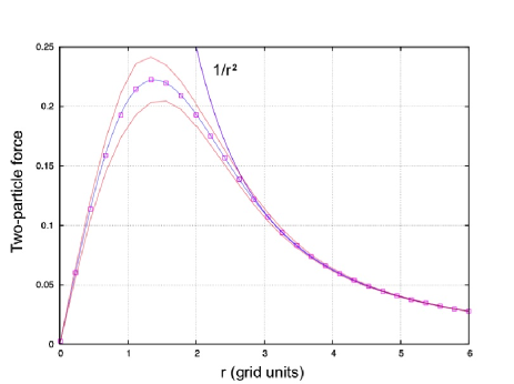
Figure 3: Orientation-averaged force between two particles as a function of separation, using digital filtering and spectral differentiation with CIC deposition as implemented in HACC. The match to the exact $1/r^{2}$ behavior is tuned to occur at a separation of three grid cells, which sets the force-matching scale, $r_{s}$. The low level of the force anisotropy noise is shown by the bracketing red lines representing the 1-$\sigma$ deviation. The solid curve is the fitting formula of Eq. 8.

The HACC long-range force solver uses only CIC mass deposition and force interpolation with a Gauss-sinc spectral filter to mimic TSC-like behavior. In addition, a fourth-order Super-Lanczos spectral differentiator (Hamming 34) is used, along with a sixth-order influence function. This approach allows the data motion to be simplified as no complicated spatial differentiation is needed. Also, by moving more of the Poisson-solve to the spectral domain, the inherent flexibility of Fourier space can be exploited. For example, the filtering is flexible and tunable, allowing careful force matching at only three grid cells. Figure 3 shows the force-matching with the spectral techniques using a pair of test particles. In this test, multiple realizations of particle pairs were taken at fixed distances, but with random orientations of the separation vector in order to sample the anisotropy imposed by the grid-based calculation of the force.

The solution of the Poisson equation in HACC’s long range force-solver is carried out using large FFTs; the corresponding spectral representation of the inverse (discrete) Laplacian is the influence function. HACC employs the following three-dimensional, sixth-order, periodic, influence function:

$$G_{6}({\bf k}) = \frac{45}{128}\Delta^{2}\left[\sum_{i}\cos\left(\frac{2\pi k_{i}\Delta}{L}\right)\right.$$ (5)

$$- \frac{5}{64}\sum_{i}\cos\left(\frac{4\pi k_{i}\Delta}{L}\right)$$

$$+ \left.\frac{1}{1024}\sum_{i}\cos\left(\frac{8\pi k_{i}\Delta}{L}\right)-\frac{2835}{1024}\right]^{-1},$$

where the sum is over the three spatial dimensions, $\Delta$ is the grid spacing, and $L$ the physical box size.

As mentioned earlier, the CIC-deposited density field is spectrally filtered using a sinc-Gaussian filter:

$$S({\bf k})=\exp{(-\left|{\bf k}\right|^{2}\sigma^{2}/4)}\left[(2/{\bf k}\Delta)\sin({\bf k}\Delta/2)\right]^{n_{s}}.$$ (6)

The aim of the filter is to reduce the anisotropy noise as well as control the matching scale where the short-range and long-range forces are matched; the nominal choices in HACC are $\sigma=0.8$ and $n_{s}=3$. This filtering reduces the anisotropy “noise” of the basic CIC scheme by better than an order of magnitude, and allows for the use of the higher-order spectral differencing scheme.

Instead of solving for the scalar potential, and then using a spatial stencil-based differentiation, HACC uses spectral differentiation within the Poisson-solve itself, using fourth-order spectral Lanczos derivatives, as previously mentioned. The (one-dimensional) fourth-order Super-Lanczos spectral differentiation for a function, $f$, given at a discrete set of points is

$$\left.\frac{\Delta f}{\Delta x}\right|_{4}\simeq$$

$$\frac{4}{3}\sum_{j=-N+1}^{N}C_{j}{\rm e}^{(2\pi jx/L)}i\frac{2\pi j\Delta}{L}\frac{\sin\left(2\pi j\Delta/L\right)}{2\pi j\Delta/L}$$

$$-\frac{1}{6}\sum_{j=-N+1}^{N}C_{j}{\rm e}^{(2\pi jx/L)}i\frac{2\pi j\Delta}{L}\frac{\sin\left(4\pi j\Delta/L\right)}{2\pi j\Delta/L},$$ (7)

where $C_{j}$ are coefficients in the Fourier expansion of $f$.

The “Poisson-solve” in the HACC code is the composition of all the kernels above in one single Fourier transform. Note that each component of the field gradient requires an independent FFT. This entails some extra work, but is a very small fraction of the total force computation, the bulk of which is dominated by the short-range solver.

An efficient and scalable parallel Fast Fourier Transform (FFT) is an essential component of HACC’s design, and determines its weak scaling properties. Although parallel FFT libraries are available, HACC uses its own portable parallel FFT implementation optimized for low memory overhead and high performance. Since slab-decomposed parallel FFTs are not scalable beyond a certain point (restricted to $N_{rank}<N_{FFT}$), the HACC FFT implementation uses data partitioning across a two-dimensional subgrid, allowing $N_{rank}<N^{2}_{FFT}$, where $N_{rank}$ is the number of MPI ranks and $N_{FFT}$ is the linear size of the 3-D array. The resulting scalable performance is sufficient for use in any supercomputer in the foreseeable future (Habib et al. 33).

The implementation consists of a data partitioning algorithm which allows an FFT to be taken in each dimension separately. The data structure of the computing nodes prior to the FFT is such as to divide the total space into regular three-dimensional domains. Therefore, to employ a two-dimensionally decomposed FFT, the distribution code reallocates the data from small ‘cubes’, where each cube represents the data of one MPI rank, to thin two-dimensional ‘pencil’ shapes, as depicted schematically in Figure 4.

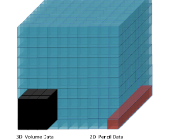
Figure 4: Data allocations for the force calculation. A three-dimensional spatial domain decomposition is used for for the force-solver, while a two-dimensional pencil structure is used for the FFT. Therefore, a reallocation of memory between the two data structures is required when carrying out either step in the computation.

Once the distribution code has formed the pencil data decomposition, a one-dimensional FFT can be taken along the long dimension of the pencil. Moreover, the same distribution algorithm is employed to carry out the remaining two transforms by redistributing the domain into pencils along those respective dimensions. The transposition and FFT steps are overlapped and pipelined, with a reduction in communication hotspots in the interconnect. Lastly, the dataset is returned to the three-dimensional decomposition, but now in the spectral domain. Pairwise communication is employed to redistribute the data, and has proven to scale well in our larger simulations. A demonstration of this is provided by the Blue Gene/Q sytems, where we have run on up to $\sim 1.5$ million MPI ranks (Habib et al. 33). As the grid size is increased on a given number of processors, the communication efficiency (i.e., the fraction of time spent communicating data between processors), remains unchanged. This is an important validation of our implementation design, as the communication cost of the algorithm must not outpace the increase in local computation performance when scaling up in size. Further details of the parallel FFT implementation will be presented elsewhere.

2.4 The Short-Range Force

The total force on a particle is given by the vector sum of two components: the long-range force and the short-range force. At distances greater than the force-matching scale, only the long-range force is needed (at these scales, the (filtered) PM calculation is an excellent approximation to the desired Newtonian limit, see Figure 3). At distances less than the force-matching scale, $r_{s}$, the short-range force is given by subtracting the residual filtered grid force from the exact Newtonian force.

To find the residual filtered PM force, we compute it numerically using a pair of test particles (since in our case no analytic expression is available), evaluating the force at many different distances at a large number of random orientations. The results are fit to an expression that has the correct asymptotic behaviors at small and large separation distances (Cf. Dubinski et al. 26). We used the particular form:

$$f_{grid}(r) = \frac{1}{r^{2}}\tanh(br)-\frac{b}{r}\frac{1}{\cosh^{2}(br)}$$ (8)

$$+ cr(1+dr^{2})\exp(-dr^{2})$$

$$+ e(1+fr^{2}+gr^{4}+lr^{6})\exp(-hr^{2}),$$

which, with $b=0.72$, $c=0.01$, $d=0.27$, $e=0.0001$, $f=360$, $g=100$, $h=0.67$, and $l=17$, provides an excellent match to the data from the test code (Figure 3), with errors much below $0.1\%$. At very small distance scales, the gravitational force must be softened, and this can be implemented using Plummer or spline kernels (see, e.g., Dehnen 20).

The force expression, Eq. (8), is complex and to implement faster force evaluations one can either employ look-ups based on interpolation or a simpler polynomial expression. The communication penalty of look-ups can be quite high, whereas an extended dynamic range is difficult to fit with sufficiently low-order polynomials. In our case, the choice of a short matching scale, $r_{s}$, enables the use of a fifth-order polynomial approximation, which can be vectorized for high performance.

Depending on the target architecture, HACC uses two different short-range solvers, one based on a tree algorithm, the other based on a direct particle-particle interaction (P³M). Tree methods are employed on non-accelerated systems, while both P³M and tree methods can be used on accelerated systems. HACC uses an RCB tree in conjunction with a highly-tuned short-range polynomial force kernel. (An oct-tree implementation also exists, but is not the current production version.) The implementation of the RCB tree, although not the force evaluation scheme, generally follows the discussion in [29]. (Multiple RCB trees are used per rank to enhance parallelism, as described in Section 3.1.) Two core principles underlie the high performance of the RCB tree’s design (Habib et al. 33).

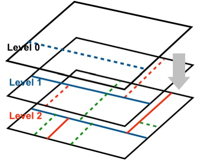
Figure 5: Notional sketch of an RCB tree spatial domain splitting for a 2-D particle distribution, following [29]. The cut-lines (planes in 3-D) go through the particle distribution center of mass in a cell – rather than the median – and are perpendicular to the longest cell side. The criterion for the maximal level of the tree depth depends on the details of the computational architecture (see text).

Spatial Locality. The RCB tree is built by recursively dividing particles into two groups. The dividing line is placed at the center of mass coordinate perpendicular to the longest side of the box (Figure 3.1). Once the line of division is chosen, the particles are partitioned such that particles in each group occupy disjoint memory buffers. Local forces are then computed one leaf node at a time. The net result is that the particle data exhibits a high degree of spatial locality after the tree build; because the computation of the short-range force on the particles in any given leaf node, by construction, deals with particles only in nearby leaf nodes, the cache miss rate during the force computation is very low.

Walk Minimization. In a traditional tree code, an interaction list is built and evaluated for each particle. While the interaction list size scales only logarithmically with the total number of particles (hence the overall ${\mathcal{O}}(N\log N)$ complexity), the tree walk necessary to build the interaction list is a relatively slow operation. This is because it involves the evaluation of complex conditional statements and requires “pointer chasing” operations. A direct $N^{2}$ force calculation scales poorly as $N$ grows, but for a small number of particles, a thoughtfully-constructed kernel can still finish the computation in a small number of cycles. The RCB tree exploits our highly-tuned short-range force kernels to decrease the overall force evaluation time by shifting workload away from the slow tree-walking and into the force kernel. Up to a point, doing this actually speeds up the overall calculation: the time spent in the force kernel goes up but the walk time decreases faster. Obviously, at some point this breaks down, but on many systems, tens or hundreds of particles can be in each leaf node before the crossover is reached. We point out that the force kernel is generally more efficient as the size of the interaction list grows: the relative loop overhead is smaller, and more of the computation can be done using unrolled vectorized code.

In addition to the performance benefits of grouping multiple particles in each leaf node, doing so also increases the accuracy of the resulting force calculation: The local force is dominated by nearby particles, and as more particles are retained in each leaf node, more of the force from those nearby particles is calculated exactly. In highly-clustered regions (with very many nearby particles), the accuracy can increase by several orders of magnitude when keeping over 100 particles per leaf node.

The P³M implementation within HACC follows the standard method of building a chaining mesh to control the number of particle-particle interactions (Hockney & Eastwood 41). This algorithm is used within HACC when working with accelerated systems. We defer further details regarding the architecture-specific implementation of the short-range force to Section 3, where the different alternatives are covered separately.

2.5 Time-Stepping

The time-stepping in HACC is based on the widely employed symplectic scheme, as used, e.g., in the IMPACT code (Qiang et al. 59), the forerunner of MC² (Mesh-based Cosmology Code, see, e.g., Heitmann et al. 35), in turn the PM precursor of HACC. The basic idea here is not to finite-difference the equations of motion, but to view evolution as a symplectic map on phase space. Symplectic integration in HACC approximates the full evolution to second order in the time-step by composing elementary maps using the Campbell-Baker-Hausdorff series expansion (Sternberg 64). In PM mode, the elementary maps are the ‘stream’ and ‘kick’ maps $M_{1}=\exp(-t\hat{H}_{1})$ and $M_{2}=\exp(-t\hat{H}_{2})$ corresponding to the free particle (kinetic) piece and the one-particle effective potential in the Hamiltonian, respectively. In the stream map, the particle position is drifted using its known velocity, which remains unchanged; in the kick map, the velocity is updated using the force evaluation, while the position remains unchanged. A symmetric ‘split-operator’ symplectic step $M_{1}(t/2)M_{2}(t)M_{1}(t/2)$ is termed SKS (stream-kick-stream); a KSK step is another way to implement a second-order symplectic integrator. (In the presence of explicitly time-dependent Hamiltonan pieces, the map evaluations have to be implemented at the correct times to maintain second-order accuracy.)

In the presence of both short and long-range forces, we split the Hamiltonian into two parts, $H_{1}=H_{sr}+H_{lr}$ where $H_{sr}$ contains the kinetic and particle-particle force interaction (with an associated map $M_{sr}$), whereas, $H_{2}=H_{lr}$ is just the long range force, corresponding to the map $M_{lr}$. Since the long range force varies relatively slowly, we construct a single time-step map by subcycling $M_{sr}$:

$$M_{full}(t)=M_{lr}(t/2)(M_{sr}(t/n_{c}))^{n_{c}}M_{lr}(t/2),$$ (9)

the total map $M_{sr}$ being a usual second-order symplectic integrator. This corresponds to a KSK step, where the S is not an exact stream step as in the PM case, but has enough $M_{sr}$ steps composed together to obtain the required accuracy. For typical problems the number, $n_{c}$, of short time steps for each long time step will range between 3-10, depending on accuracy requirements.

Because the late-time distribution of particles is highly clustered, there can be a substantial advantage in using different (synchronized) local time steps down to the single-particle level. Although HACC is currently designed for a regime where extreme dynamic range is not needed, as in treating the innermost part of galaxy halos or in tracking orbits around black holes – where this advantage is most felt (e.g., Power et al. 57) – the automatic density information available in the short-range force solvers is used to enable multi-level time-stepping, resulting in speed-ups by a factor of 2-3, with only small effects on the accuracy. More on this topic can be found in Section 3.

2.6 Code Units

HACC uses comoving coordinates for positions and velocities. The actual internal representation of all variables is in the dimensionless form:

$${\bf x}\equiv x_{0}{\bf{\tilde{x}}},~{}~{}t\equiv\tilde{t}/H_{0},~{}~{}\rho\equiv\tilde{\rho}\rho_{b},$$ (10)

where the fundamental scaling length, $x_{0}$, is the length of a single grid cell of the long-range force PM-solver, $L/(N_{g}-1)$, where $L$ is the box-size and $N_{g}$ is the number of grid points in a single dimension, $H_{0}$ is the current value of the Hubble parameter, and the background mass density, $\rho_{b}=3H_{0}^{2}\Omega_{0}/(8\pi Ga^{3})$. HACC uses powers of the scale factor, $a(t)^{\alpha}$, as the actual evolution variable, with a nominal default value of $\alpha=1$; time-stepping is performed using the variable $y=a^{\alpha}$, $d/d\tilde{t}=(\alpha yH/H_{0})d/dy$.

2.7 Memory Management

Besides easy portability between different architectures, another very important feature of HACC is its highly optimized memory footprint. Pushing the simulation limits in large-scale structure formation problems means running simulations with as many particles as possible, and this often implies running as close as possible to the memory limit of the machine. As a result, memory fragmentation becomes a serious problem. To make matters worse, HACC is required to allocate and free different data structures during different parts of each time step because there is not enough available memory to hold all such structures at the same time. Furthermore, many of these data structures, such as the RCB tree used for the short-range force calculation, have sizes that change dynamically with each new time step. This, combined with other allocations from the MPI implementation, message printing, file I/O, etc. with lifetimes that might outlast a time-step phase (e.g. long-range force computation, short-range force computation, in situ analysis), is a recipe for fatal memory fragmentation problems – problems that we actually encountered on the Blue Gene/Q systems.

To mitigate this difficulty we have implemented a specialized pool allocator called Bigchunk. This allocator grabs a large chunk of memory, and then distributes it to various other subsystems. During the first time step, Bigchunk acts only as a wrapper of the system’s memory allocator, except that it keeps track of the total amount of memory used during each phase of the time step. Before the second time step begins, Bigchunk allocates an amount of memory equal to the maximum used during any phase of the previous time step plus some safety factor. Subsequent allocations are satisfied using memory from the ‘big chunk’, and all such memory is internally marked as free after the completion of each time-step phase. This en-masse deallocation, the only kind of deallocation supported by Bigchunk, allows for an implementation that has minimal overhead, and the time it takes to allocate memory from Bigchunk is very small compared to the speed of the system allocator. Because the Bigchunk memory is not released back to the system, memory fragmentation no longer fatally affects the ability of the time-step phases to allocate their necessarily-large data structures.

The persistent state information in the simulation is carried by the particle attributes. While the number of particles in each MPI rank’s (overloaded) spatial sub-volume is similar, structure formation implies some variance. Once the overload cache is filled, the (total) number of particles on a rank is fixed until the cache is emptied and refreshed, at which point the number of particles on each rank can change. In order to avoid memory fragmentation with persistent information we must anticipate the maximum number of particles any rank will need during the course of a simulation run and allocate that amount of memory for particle information at the start, before any other significant memory allocation occurs. We estimate the maximum number of particles by choosing a maximum representative volume from which bulk motion could move all of the particles into a rank’s (overloaded) sub-volume and multiply that volume by the average particle density. The actual memory allocations are monitored during runtime, allowing for adjustments to be made while the code is running. In practice for the sub-volumes with side lengths that are at least several tens of Mpc this results in allocating memory for an additional skin of particles that is 6-10 Mpc thick. HACC prints a memory diagnostic at each time step to indicate the extrema of particle memory usage across all ranks, and the amount of extra memory can be adjusted when restarting the code if the initial estimate appears to be insufficient for later times. In addition to the space required for the actual particle information, we also allocate an array of integers to represent a permuted ordering of the particles and a scratch array large enough to hold any single particle attribute. These enable out-of-place re-ordering of the particle information one attribute at a time without additional memory allocation.

2.8 I/O Strategy

A plurality of I/O strategies are needed for different use cases, machine architectures, and data sizes because no single I/O strategy works well under all of these conditions. Our three main approaches are described below.

One file per process. Using one output file per process (i.e. MPI rank) is the simplest I/O strategy, and continues to provide the best write bandwidth compared to any other strategy. Because every process writes into a separate file, after file creation, there is no locking or synchronization needed in between processes. Unfortunately, while simple and portable, one file per process only works for a modest number of processes (typically less than 10,000). No file system can manage hundreds of thousands of files that would result from checkpointing a large-scale run with one file per process. Additionally, as a practical matter, managing hundreds of thousands of files is cumbersome and error-prone. Finally, even when the number of files is reasonable, reading the stored data back into a different number of processes than used to write the data requires redistribution. This happens when the output is used for analysis on a smaller cluster (or machine partition), or for visualization. In such cases, the required reshuffling of all of the data in memory is equivalent to the aggregation done by more complex collective I/O strategies and cancels out the simplicity of the one file per process approach. For improved scalability and flexibility, HACC supports the following additional I/O strategies.

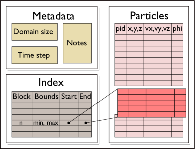
Figure 6: File schema for analysis output enables spatial queries of particle data in a high-level, portable, self-describing format.

Many processes per file. The default I/O strategy used by HACC, called GenericIO, partitions the processes in a system-specific manner, and each partition writes data into a custom self-describing file format. Each process writes its data into a distinct region of the file in order to reduce contention for file-system-level page locks. Within the region assigned to each process, each variable is written contiguously. On modern supercomputers, such as IBM Blue Gene and Cray X series machines, dedicated I/O nodes execute special I/O forwarding system software on behalf of a set of compute nodes. For example, on IBM Blue Gene/Q systems, one I/O node is assigned to 128 compute nodes. By writing one file per I/O node, the total number of files is reduced by at least the ratio of compute nodes to I/O nodes, and a high percentage of the peak available bandwidth can be captured by the reading and writing processes. By partitioning the processes by I/O-node assignment and providing each process with a disjoint data region, we are taking advantage of the technique successfully used by the GLEAN I/O library (Vishwanath et al. 70) on the Blue Gene/P and Blue Gene/Q systems. The I/O implementation can use MPI I/O, in either collective or non-collective mode, or (non-collective) POSIX-level I/O routines.

Importantly, 64-bit cyclic-redundancy-check (CRC) codes are computed for each variable for each rank, and this provides a way to validate data integrity. This detects corruption that occurs while the data is stored on disk, while files are being transferred in between systems, and while being transmitted within the storage subsystem(s). During a recent run which generated  100 TB of checkpoint files, a single error in a single variable from one writing process was detected during one checkpoint-reading process, and we were able to roll-back to a previous checkpoint and continue the simulation with valid data. Furthermore, over the past two years, CRC validation has detected corrupted data from malfunctioning memory hardware on storage servers, misconfigured RAID controllers and bugs in (or miscompiled) compression libraries. The probability of seeing corrupt data from any of these conditions is small (even while they exist), and overall, modern storage subsystems are highly reliable, but when writing and reading many petabytes of data at many facilities the probability of experiencing faults is still significant. The CRC64 code is in the process of being transformed into an open-source project.

An example of GenericIO performance under production conditions on the Blue Gene/Q system Mira is given in Table 1. In tests, I/O performance very close to the peak achievable has been recorded. Under production conditions, we still achieve about two-thirds of the peak performance.

A single file using parallel netCDF. When peak I/O performance is not required, and the system’s MPI I/O implementation can deliver acceptable performance, we can make use of a parallel-netCDF-based I/O implementation (Li et al. 50). The netCDF format is used by simulation codes from many different science domains, and readers for netCDF have been integrated with many visualization and analysis tools. Because netCDF has an established user community, and will likely be supported into the foreseable future, writing data into a netCDF-based format should make distributing data generated by HACC to other outside groups easier than if only custom file formats were supported.

The file schema that we developed for the parallel netCDF format is shown in Figure 6. As the figure shows, particles are organized and indexed according to the spatial subdomains (blocks) of the simulation, one block per process. The spatial extents of each block are also indexed.

Currently, three modes of reading the parallel netCDF files are supported. First, given some number of processes that need not be the same as the number of blocks, particles can be redistributed uniformly among the new number of processes while being read collectively. Second, the particles in a single block can be retrieved given the block ID. Third, particles in a desired bounding box can be retrieved. The queried bounding box need not match the extents of any one block and particles overlapping several blocks may be retrieved in this manner.

The performance for writing the parallel netCDF output is shown in Table 2. These tests were run on Hopper (Cray XE6) at the National Energy Research Scientific Computing Center (NERSC) with a Lustre file system. Because the file system is shared by all running jobs, performance results will vary due to resource contention; the values in Table 2 are the means of four runs for each configuration.

To put these results in perspective, consider the last row of Table 2. The peak performance expected for the number of object storage targets (OSTs, 128 in this case) is approximately 26.7 GiB/s (1 GiB = $2^{30}$ = 1,073,741,824 bytes). This value represents ideal conditions of writing large amounts of data to one file per OST. In contrast, our strategy uses one shared file with collective I/O aggregation and a high-level format with index data in addition to raw particle arrays. Even so, we achieve 56% of the peak ideal bandwidth.

Table 1: GenericIO Performance (production runs on IBM Blue Gene/Q)

No. Particles	No. Processes	File size (GiB)	Write time (s)	Write Bandwidth (GiB/s)
$1024^{3}$	512	43.8	22.0	1.90
$3200^{3}$	16384	1332.4	99.0	12.88
$10240^{3}$	262144	43821.6	380.5	109.9

Table 2: Parallel NetCDF Performance (test runs on Cray XE6)

No. Particles	No. Processes	File size (GiB)	Write time (s)	Write Bandwidth (GiB/s)
$512^{3}$	64	4.6	3.54	1.30
$1024^{3}$	512	36	14.34	2.51
$2048^{3}$	4096	288	19.10	15.1

3 Short-Range Force: Architecture Specific Implementations

In this section we go over the choice of algorithms deployed as a function of nodal architecture, as well as the corresponding optimizations implemented so far – performance optimization is a continuous process.

3.1 Non-Accelerated Systems: The RCB Tree

In order to evaluate the short-range force on non-accelerated systems, such as the Blue Gene/Q, HACC uses an RCB tree in conjunction with a highly-tuned short-range polynomial force kernel, as has been discussed in Section 2.4.

An important consideration in this implementation is the tree-node partitioning step, which is the most expensive part of the tree build. The particle data is stored as a collection of arrays – the so-called structure-of-arrays format. There are three arrays for the three spatial coordinates, three arrays for the velocity components, in addition to arrays for mass, a particle identifier, etc. Our implementation in HACC divides the partitioning operation into three phases. The first phase loops over the coordinate being used to divide the particles, recording which particles will need to be swapped. Next, these prerecorded swapping operations are performed on six of the arrays. The remaining arrays are identically handled in the third phase. Dividing the work in this way allows the Blue Gene/Q hardware prefetcher to effectively hide the memory transfer latency during the particle partitioning operation and reduces expensive read-after-write dependencies.

The premise underlying the multilevel timestepping scheme (Section 2.5) is that particles in higher density regions will require finer short-range time steps. A local density estimate can be trivially extracted from the same RCB tree constructed for evaluating the short-range interparticle forces. Each “leaf node” in the RCB tree holds some number of particles, the bounding box for those particles has already been computed, and a constant density estimate is used for all particles within the leaf node’s bounding box. Because the bounding box, and thus the density estimate, changes as the particles are moved, the timestepping level assigned to each leaf node is fixed when the tree is constructed. This implies that, after particles have been moved, the leaf-node bounding boxes may overlap. The force-evaluation algorithm is insensitive to these small overlaps, and the effect on the efficiency of the force calculation is apparently negligible.

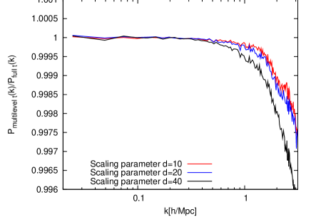
Figure 7: Comparison of the multi-level time stepper with different values for $d$ [see Eq. (11)] versus 5 sub-cycle steps for each particle. Shown is the ratio of the final power spectra for a small test problem (256 $h^{-1}$Mpc, 256³ particles), going out to the particle Nyquist wave number. The multi-level time step approach leads to a speed-up of the full simulation by a factor of $\sim$2, with only a negligible change in the error.

In between consecutive long-range force calculations, each particle is operated on by the kick (velocity update) and stream (position update) operators of the short-range force. If a particle, based on the density of its leaf node at the beginning of the subcycle, is evolved using $n$ kicks, then it needs to be acted on by $2n$ stream operators each evolving the particle by $dt/2n$. To ensure time synchronization, these stream operators are further split such that all particles are acted on by the same number of stream operators. The number of kicks used for particles in a leaf node is determined by:

$$l=\left\lfloor\frac{\rho}{\rho_{0}}\right\rfloor/d+1,$$ (11)

where $d$ is an adjustable linear scaling parameter. In addition, the maximum level is capped by an additional user-provided parameter. We show examples of accuracy control in the multi-level time stepping scheme in Figures 7 – 11.

In Figure 7, we compare the power spectrum obtained from a simulation with 5 sub-cycle steps for each particle with a result that was obtained in the following way: 5 sub-cycles per step per particle are used until $z=1$; since the clustering at that point is still modest, this point is reached relatively quickly. After $z=1$ we evolve each particle with at least 2 sub-cycles and allow – depending on the density – two more levels of sub-cycling. In this test, setting the scaling parameter $d$ to 20 or 10 leads to accurate results, better than 0.2% out to the particle Nyquist wavenumber, $k_{\rm Ny}\equiv\pi/\Delta$, where $\Delta$ is the initial inter-particle separation (the test case used 256³ particles in a 256 $h^{-1}$Mpc volume with 500 PM steps.) In precision cosmology applications, one desires better than $1\%$ accuracy, and this is attained at wavenumbers less than $k_{\rm Ny}/2$ (Heitmann et al. 37). Consequently, the current error limits are comfortably wihtin the required bounds, the error at $k_{\rm Ny}/2$ being only $\sim 0.05\%$. Using the multi-level stepping can speed up the simulation by a factor of two (changing $d$ in the range shown leaves the performance unaffected). We have carried out a suite of convergence tests, concluding that the setting with $d=20$ satisfies our accuracy requirements.

At much smaller length scales, the power spectrum test above can be augmented by checking the stability of small scale structures in the halos as the adaptive time-stepping parameters are varied. As typical examples thereof, we show results for the largest and second-largest halos (identified using a ‘friends-of-friends’ or FOF algorithm) in the same simulation discussed above in Figures 8 – 11. The halo density field is computed via a tessellation-based method in three dimensions and then projected onto a two-dimensional grid; details of this implementation will be presented elsewhere (Rangel et al. 58). The angle-averaged (spherical) density profiles are also shown in Figures 9 and 11. As can be seen from these results, aside from trivial differences due to the FOF linking noise, the halo substructure depends relatively mildly on the choice of the values of the scaling parameter, $d$, over the chosen ranges used.

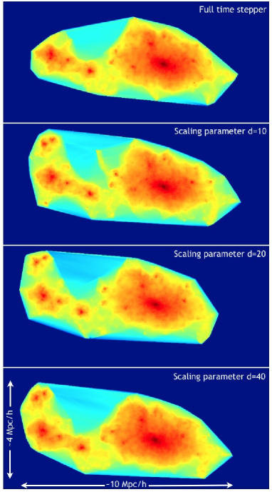
Figure 8: Projected density field from a Delaunay tessellation-based density estimator of the largest (FOF, link length, $b=0.2$) halo at $z=0$ for the same run as in Figure 7, with different values for $d$. Minor variations in the outskirts of the halos are due to FOF linking ‘noise’.

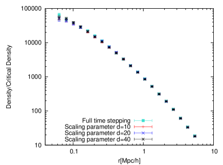
Figure 9: Density profile for the halo depicted in Figure 8 at corresponding values of the scaling parameter, $d$.

Figure 10: Same as in Figure 8 for the second largest halo.

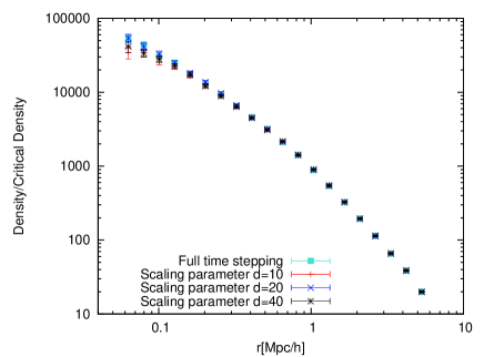
Figure 11: Same as Figure 9 for the second-largest halo.

Aside from optimizing the number of force evaluations, one also has to minimize the time spent in evaluating the force kernel. This is a function of the design of the compute nodes. Here we provide a description of the Blue Gene/Q-specific short-range force kernel and how it is optimized. (Very similar implementations were carried out for Cray XE6 and XC30 systems.) As mentioned earlier, the compactness of the short-range interaction (Cf. Section 2.3), allows the kernel to be represented as

$$f_{SR}(s)=(s+\epsilon)^{-3/2}-f_{grid}(s)$$ (12)

where $s={\mathbf{r}}\cdot{\mathbf{r}}$, $f_{grid}(s)$ is a 5-th order polynomial in $s$, and $\epsilon$ is a short-distance cutoff (Plummer softening). This computation must be vectorized to attain high performance; we do this by computing the force for every neighbor of each particle at once. The list of neighbors is generated such that each coordinate and the mass of each neighboring particle is pre-generated into a contiguous array. This guarantees that 1) every particle has an independent list of particles and can be processed within a separate thread; and 2) every neighbor list can be accessed with vector memory operations, because contiguity and alignment restrictions are taken care of in advance. Every particle on a leaf node shares the interaction list, therefore all particles have lists of the same size, and the computational threads are automatically balanced.

The filtering of $s$, i.e., checking the short-range condition, can be processed during the generation of the neighbor list or during the force evaluation itself; since the condition is likely violated only in a number of “corner” cases, it is advantageous to include it into the force evaluation in a form where ternary operators can be combined to remove the need of storing a value during the force computation. Each ternary operator can be implemented with the help of the fsel instruction, which also has a vector equivalent. Even though these alterations introduce an (insignificant) increase in instruction count, the entire force evaluation routine becomes fully vectorizable.

There is significant flexibility in choosing the number of MPI ranks versus the number of threads on an individual Blue Gene/Q node. Because of the excellent performance of the memory sub-system, a large number of OpenMP threads – up to 32 per node – can be run to optimize performance. Concurrency in the short-range force evaluation is exposed by, first, building a work queue of leaf-node-vs-tree interactions, and second, executing those interactions in parallel using OpenMP’s dynamic scheduling capability. Each work item incorporates both the interaction-list building and the force calculation itself for each leaf node’s particles.

To further increase the amount of parallel work, HACC builds multiple RCB trees per rank. First, the particles are sorted into fixed bins, where the linear size of each bin is roughly the scale of the short-range force. An RCB tree is then constructed within each bin, and because this process in each bin is independent of all other bins, this is done in parallel. This parallelization of the tree-building process provides a significant performance boost to the overall force computation. When the force on the particles in each leaf node is computed, not only must the parent tree be searched, but so must the other 26 neighboring trees. Because of the limited range of the short-range force, only nearest neighbors need to be considered. While searching many neighboring trees adds extra expense, the trees are individually not as deep, and so the resulting walks are less expensive. Also, because we distribute ‘(leaf node, neighboring tree)’ pairs among the threads, this scheme also increases the amount of available parallelism post-build (which helps with thread-level load balancing). All told, using multiple trees in this fashion provides a significant performance advantage over using one large tree for the entire domain.

3.2 Cell-Accelerated Systems

The first version of HACC was originally written for the IBM PowerXCell 8i-accelerated hardware of Roadrunner, the first machine to break the Petaflop barrier. This architecture posed three critical challenges, all of which continue to be faced in one way or the other on all accelerated systems. A more detailed description of the Cell implementation and the Roadrunner architecture is given in [32]. (See also Swaminarayan 66.)

The three challenges for a Roadrunner-style architecture are as follows. (i) Memory Balance. The machine architecture (Figure 12) has a top layer of conventional multi-core processors (in this case, two dual-core AMD Opterons) to which are attached IBM PowerXCell 8i Cell Broadband Engines (Cell BEs) via an eight-lane PCI-E bus. The relative performance of the Opterons is small compared to that of the Cell BEs, by roughly a factor of 1:20, but they carry half the memory and possess access to a communication fabric that is balanced to their level of computational performance. For large-scale N-body codes, memory is a key limiting factor, therefore the code design must make the best use possible of the CPU layer (this situation continues in current and future accelerated systems, as discussed further below). (ii) Communication Balance. The Cell BEs dominate the computational resource, but are starved for communication, due to the relatively slow PCI-E link to the host CPU (Figure 12). From the point of view of the compute/communication ratio, such a machine is 50-100 times out of balance. We note that this situation also continues to hold in the current generation of accelerated systems such as CPU/GPU or CPU/Xeon Phi machines: The computational approach taken must therefore maximize computation for a given amount of data motion. (iii) Multiple Programming Models. Accelerated systems have a multi-layer programming model. On the CPU level, standard languages and interfaces can be used (HACC uses C/C++/MPI/OpenMP) but the accelerator units often have a hardware-specific programming paradigm. (Although attempts to overcome this gap now exist, the results – in actual practice – are not yet compelling.) For this reason, it is desirable to keep the code on the accelerator (the Cell BE in this case) as simple as possible and avoid elaborate coding. In addition, it also proved advantageous to keep the data structures and communication patterns on the Cell BE as straightforward as possible to optimize computational efficiency.

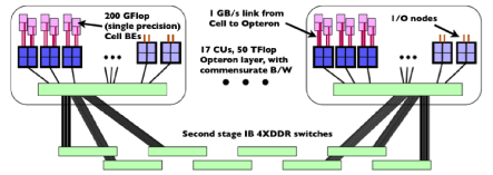
Figure 12: Roadrunner architecture schematic: The accelerator units (IBM Cell BEs) are shown in pink, the CPUs (AMD Opterons) in blue, and the (fat tree) interconnect in green. Note that communication across the Cell BE layer has to proceed indirectly, passing through the CPU layer.

With these challenges in mind, HACC is matched to the machine architecture as follows: At the first level of code organization, the medium/long range force is handled by the FFT-based method that operates at the Opteron layer, as for all other architectures. At this layer, only grid information is stored and manipulated (except when carrying out analysis steps). Particles live only at the Cell layer. There is a rough memory balance between the grid and particle data, matching well to the memory organization on the machine, and combating the first challenge mentioned above. The particle-grid deposition and grid-particle interpolation steps are performed at the Cell layer with only grid information passing between the two layers. This compensates for the limited bandwidth available between the Cell BEs and the Opterons. The local force calculations reside at the Cell level. This addresses the second challenge, as aided by the particle overloading discussed in Section 2.2. Because implementing complicated data structures at the Cell level is difficult, and conditionals are best avoided, our choice for the local force solve is a direct particle-particle interaction. To make this interaction more efficient, we use a chaining mesh to control the number of interactions (see, e.g., Hockney & Eastwood 41). This leads to an efficient, hardware-accelerated P³M algorithm, thereby overcoming the third challenge (Pope et al. 56).

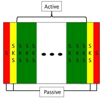
Figure 13: Figure illustrating the partitioning of active and passive particles. The outside (red) slabs of data are solely streamed, and the yellow and green slabs calculate the full short range (SKS) force. In analogy, the red and yellow slabs can be thought of as the overloaded ‘passive’ particles, and the green slabs are ‘active’, which are correctly updated. The finest partitioning is achieved in 5 slab blocks, where there is only one (green) corrected slab updated.

3.3 GPU-Accelerated Systems

As already discussed above, some of the challenges for GPU-accelerated systems are very similar in spirit to those for Cell-accelerated systems. The low-level GPU programming model (OpenCL or CUDA) adds another layer of complexity and the compute to communication balance is heavily skewed towards computing. One major difference between the two architectures is the memory balance: While on the Cell-accelerated systems the Cell layer has the same amount of memory as the CPU layer, this is generally not the case for CPU/GPU systems. For example, the Cray XK7 system, Titan, at Oak Ridge, has 32 GB of host-side memory on a single node, with only 6 GB of GPU memory. This adds yet another challenge, that of memory imbalance. We have overcome this by partitioning the local data into smaller overlapping blocks, which can fit on device memory. Very similar in spirit to particle overloading, the boundaries of the partitions are duplicated, such that each block can be evolved independently. We emphasize again that the long/medium range calculations on this architecture remain unchanged, and only the short-range force kernel needs to be optimized.

The data partitioning is illustrated in Figure 13. We utilize a two-dimensional decomposition of data blocks, which are in turn composed of slabs that are spatially separated by the extent of the short-range force – roughly 3 grid cells (see Figure 3). In complete analogy to particle overloading, the data blocks are composed of ‘active’ particles (green) that are updated utilizing the ‘passive’ particles (yellow and red) from the boundary. The (red) edge slabs are solely streamed, as opposed to performing the full SKS time stepping described in Section 2.5. This mediates the error inflow on these passive particles, as they can only “see” the interior particles within the domain. We note that since the data has been decomposed into smaller independent work items, these blocks can now be communicated to any nodes that have the available resources to handle the extra workload. Hence, this scheme provides for a straightforward load-balancing algorithm by construction. Details of the error analysis and load balancing schemes will be described in an upcoming paper devoted to the GPU implementation of HACC [28].

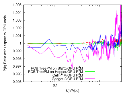
Figure 14: Ratio of the power spectra from four different runs with respect to the HACC GPU implementation, time-stepping conditions for all HACC versions held fixed. The comparison shows the Blue Gene/Q PPTreePM version (red solid), the X86 TreePM version run on a Cray XE6 (green dashed), and the GPU P³M version (blue short-dashed). We also show the comparison with a Gadget-2 run. The agreement is very good – the TreePM runs agree with the GPU version of HACC to better than 0.1% up to the particle Nyquist wavenumber. The level of agreement with Gadget-2 is noteworthy because it is a completely independent code.

4 Code Verification and Testing

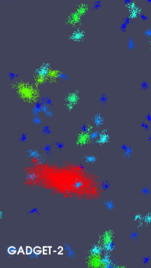
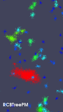
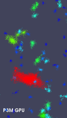
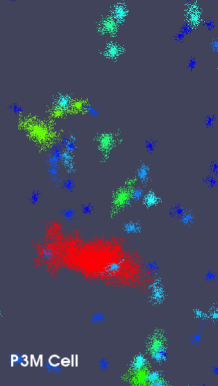
Figure 15: Comparison of halo particles between Gadget-2 (left) and three HACC implementations, the PPTreePM version (Cray XE6), the GPU version, and the Cell version. The smallest halos shown consist of 100 particles (dark blue), the largest halos have up to $\sim$19,000 particles (red). Green colors show halos in the few thousand particle range. If a dark blue halo is missing in one of the images, this is due to the mass cut at 100 particles (the halo has fallen below a threshold, but actually exists). The linking length in the comparison was chosen to be $b=0.168$. The very good level of overall agreement is clearly evident.

Table 3: Comparison of a sample of halo statistics from the code comparison runs, as extracted from the ParaView analysis. The total number of halos is N_h, the number of particles, N_p, the FOF link length, $b$, and the velocity dispersion is denoted by $\sigma_{v}$.

	Gadget-2	RCBTreePM	P3M-GPU	P3M-Cell
Nh, $b=0.2$	9707	9638	9636	9634
Nh, $b=0.168$	8817	8734	8732	8728
Np, most massive halo, $b=0.2$	22,587	21,802	22,114	22,240
Np, most massive halo, $b=0.168$	18,728	18,656	19,047	19,088
range of $\sigma_{v}$ [km/s], $b=0.2$	[132.4, 1109.9]	[134.4, 1126.2]	[134.2, 1101.3]	[133.2, 1101.16]
range of $\sigma_{v}$ [km/s], $b=0.168$	[133.5, 1144.5]	[145.5, 1141.3]	[151.3, 1128.6]	[143.7, 1146.7]

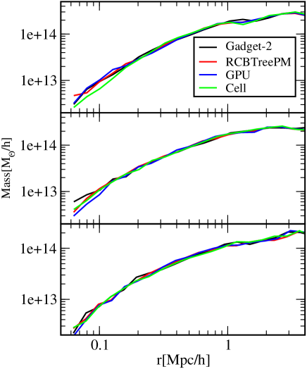
Figure 16: Comparison of the mass profiles of the three biggest halos in the test simulation, showing close agreement within the binning shot noise scatter (larger at smaller radii).

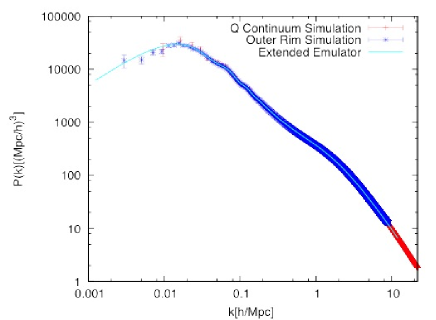
Figure 17: Matter fluctuation power spectra from the Outer Rim and Q Continuum simulations at $z=0$. The solid curve is the prediction from the extended Coyote emulator of [38]. The agreement across the two runs is at the fraction of a percent level, while the agreement with the emulator is at the 2% level, which is the estimated emulator accuracy.

HACC has been subjected to a large number of standard convergence tests (second-order time-stepping, halo profiles, power spectrum measurements, etc.). In this section we focus mostly on a subset of HACC test results using the setup of the code comparison project, originally carried out in [35]. In that work, a set of initial conditions was created for different problems (mainly different volumes) and a number of cosmological codes were run on those, all at their nominal default settings. The final outputs were compared by measuring a variety of statistics, including matter fluctuation power spectra, halo positions and profiles, and halo mass functions. The initial conditions and final results from the tests are publicly available and have been used subsequently by other groups for code verification, e.g for Gadget-2 [63], and most recently for Nyx [2]. In addition, we will also show some results from recently carried out large-scale simulations.

We first restrict attention to the larger volume simulation (256 $h^{-1}$Mpc) and compare HACC results with those found for Gadget-2, as published in [63]. While the simulation is only modest in size (256³ particles) it does present a relatively sensitive challenge and is capable of detecting subtle errors in the code under test. Not only are statistical measures such as the power spectrum robust indicators of code accuracy, but visual inspection of the particle data itself presents a quick qualitative check on code behavior and correctness; it is particularly valuable in identifying problems at early stages of code development. We use ParaView for this purpose (Woodring et al. 76).

The code comparison test was run with a force resolution of $\sim 7~{}h^{-1}$kpc, very similar to what was used in the Gadget-2 simulation. We compare results from different HACC versions (PPTreePM on the Blue Gene/Q and Hopper, P³M on a Cell-accelerated and a GPU-accelerated system) with those from Gadget-2. The result for the matter power spectrum is shown in Figure 14, where, as in Figure 7, we show results up to $k_{\rm Ny}$. All the code results are very close to each other (note the scale on the y-axis). The agreement over the full $k$-range is better than 0.5%, including Gadget-2. Considering the different implementations of force solvers and time steppers, this closeness is very reassuring, particularly as no effort was made to fine-tune the level of agreement. The TreePM versions of HACC and the CPU/GPU version agree to better than a tenth of a percent.

Next we present results from a more qualitative, but nevertheless, very detailed comparison, shown in Figure 15. In this test, we identify all particles that belong to halos with at least 100 particles per halo. This is done within ParaView, using an FOF halo finder with linking length $b=0.168$. The particles are colored with respect to halo mass. The most massive halo in the image (colored in red) has a mass of $\sim 1.6\cdot 10^{15}~{}h^{-1}$M_⊙. While there are differences in the images – as is to be expected – the overall agreement is striking. Almost all small halos exist in all images (the ones that are missing are just below the cut of 100 particles, but they do actually exist) and many of the fine details within the halo structures of the larger halos are well-matched.

The mass profiles of the three largest halos in the simulation are shown in Figure 16. The binning shot noise dominates the comparison at small radii, but beyond that the agreement is very good. Other quantitative halo comparison statistics are given in Table 3, to further illustrate the close match of the results from all of the different algorithms.

We illustrate the dynamic range and accuracy of the HACC approach by comparing results for the matter power spectrum from the ‘Outer Rim’ and ‘Q Continuum’ runs in Figure 17. The Q Continuum run on Titan had $\sim 550$ billion particles, a 1.3 Gpc box, with a mass resolution, $m_{p}\sim 10^{8}$ M_⊙, and the Outer Rim run on Mira had $\sim 1.1$ trillion particles, a 4.225 Gpc box, with a mass resolution, $m_{p}\sim 10^{9}$ M_⊙. The numerical results (run with different short-range force algorithms) agree to fractions of a percent, and agree at the 2% level with the (extended) Coyote emulator predictions of [38], which is at the level of accuracy expected from the emulator.

Finally, we show results for the halo mass function at very large simulation scales illustrating excellent agreement across different sized simulations carried out using different short-range force implementations. Figure 18 shows the (FOF, $b=0.168$) halo mass function at $z=1$ resulting from three different simulations with the same cosmology, (i) a run from the Mira Universe suite ($\sim 30$ billion particles, 2.1 Gpc box, mass resolution, $m_{p}\sim 10^{10}$ M_⊙), (ii) the Q Continuum run on Titan, and (iii) the Outer Rim run on Mira.

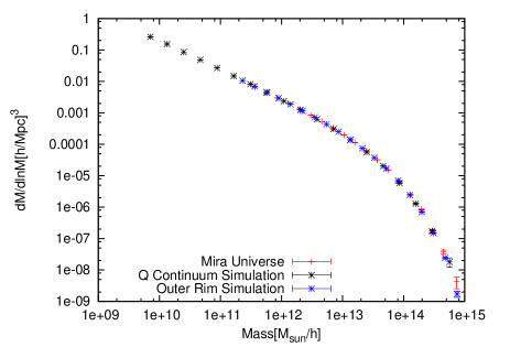
Figure 18: The (FOF, $b=0.168$) halo mass function for three large simulations run with HACC, measured at $z=1$. The box sizes range from $1-4$ Gpc and the particle number in each simulation ranges from $\sim 30$ billion to over one trillion (mass resolutions range from $\sim 10^{8}$ M_⊙ to $\sim 10^{10}$ M_⊙; for details, see text).

5 In situ Analysis Tools

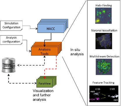
Figure 19: The in situ analysis framework provides the ability to apply various analysis tools and methods, e.g., halo finders, multistream diagnostics, feature tracking (halo merger trees), and Voronoi tessellation, and connects to run-time or postprocessing visualization tools, all while the simulation is running.

An entire suite of in situ analysis tools (CosmoTools) for HACC is under continuous development, driven by evolving science goals; CosmoTools exists in both in situ and stand-alone versions (to be used for off-line processing). The overall structure of the in situ framework is shown in Figure 19. Output from the analysis is available either at run time or for post-processing. In the former case, a ParaView server can be launched and connected to the simulation through a tool called Catalyst. In the latter case, results of the in situ analysis are written to a parallel file system and later retrieved.

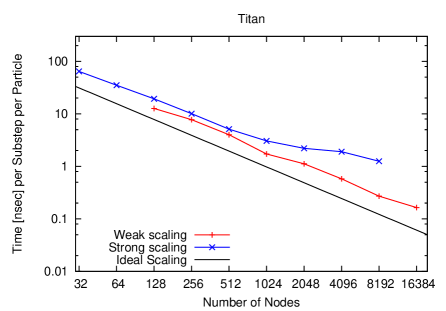
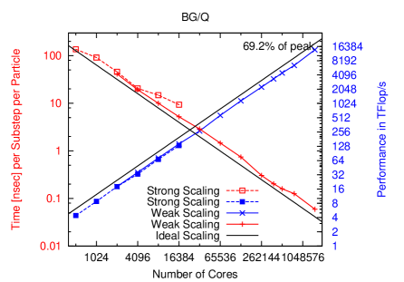
Figure 20: Early weak and strong scaling results on Titan (left panel) and from Blue Gene/Q systems (right panel, results from Mira and Sequoia). Weak scaling results are reported for a constant number of particles and physical volume per node/core (see text for details on both systems). Strong scaling results are for a fixed-size problem – 1024³ particles in a 1 $h^{-1}$Gpc box. Optimal scaling is represented by the solid black lines.

Several standard tools for the analysis of cosmological simulations are part of the in situ framework, such as halo finders (Woodring et al. 76) and merger tree constructors. The first tool to be part of this framework that works on the full particle data to produce field information is a parallel Voronoi tessellation that computes a polyhedral mesh whose cell volume is inversely proportional to the distance between particles. Such a mesh representation acts as a continuous density field that affords accurate sampling of both high- and low-density regions. Connected components of cells above or below a certain density can also approximate large-scale structures. Two important criteria for in situ analysis filters are that they should scale similarly as the simulation and have minimal memory overhead. The parallel tessellation approach meets these criteria; full details are given in [55]. The various tools can be turned on through the configuration file for HACC, and the frequency of their execution is also adjustable.

6 Selected Performance Results

HACC runs on a variety of supercomputing platforms and has scaled to the maximum size of some of the fastest machines in the world, including Roadrunner at Los Alamos, Sequoia at Livermore, Titan at Oak Ridge, Mira at Argonne, and Hopper at NERSC. We have carried out detailed scaling and performance studies on the Blue Gene/Q systems (Habib et al. 33) and on Titan; a sample of our results is presented below.

For both systems, we carried out weak and strong scaling tests. For the weak scaling tests we fix a physical volume and number of particles per node. When scaling up to more nodes, the volume and particle loading therefore increases, while the mass resolution stays constant. The wall-clock time for a run should hence stay constant if the code scales or, equivalently, the time to solution per particle per step should decrease. The absolute performance measured in TFlops per seconds will rise while the percentage per peak will stay constant. For our weak scaling tests, the particle mass is $\sim 5\cdot 10^{10}$M_⊙ and the force resolution, 6 kpc. All simulations are for a $\Lambda$CDM model. Simulations of cosmological surveys focus on large problem sizes, therefore the weak scaling properties are of primary interest.

For the weak scaling test on the Blue Gene/Q systems, we ran with 2 million particles in a $\sim$(100 $h^{-1}$Mpc)³ volume per core, using a typical particle loading in actual large-scale simulations on these systems. Tests with 4 million particles per core produce very similar results. As demonstrated in Figure 20 (right panel), weak scaling is ideal up to 1,572,864 cores (96 racks, all of Sequioa), where HACC attains a peak performance of 13.94 PFlops and parallel efficiency of $90\%$. The largest test simulation on Sequoia evolved $\sim$3.6 trillion particles and a (very high accuracy) particle substep took $\sim 0.06$ ns for the full high-resolution code. The scaling results were obtained by averaging over 50 sub-cycles.

On Titan we ran with 32 million particles per node in a fixed (nodal) physical volume of $(256~{}h^{-1}{\rm Mpc})^{3}$, representative of the particle loading in actual large-scale runs (the GPU version was run with one MPI rank per node). The results are shown in the left panel of Figure 20. In addition (not shown) we have timing results for a 1.1 trillion particle run, where we have kept the volume per node the same but increased the number of particles per node by a factor of two to 64.5 million. As for the Blue Gene/Q systems, HACC weak-scales essentially perfectly up to the full machine.

For the strong scaling tests, we chose the same problem size on both systems, a (1000 $h^{-1}$Mpc)³ volume with 1024³ particles. This is a rather small problem and strong scaling is expected to break down at some point. The results for both systems are shown in Figure 20 – the strong scaling regime is remarkably large. On the Blue Gene/Q system, we demonstrate strong scaling between 512 and 16384 cores (with somewhat degraded performance at the largest scale). For Titan, we increase the number of nodes for this problem from 32 to 8192, almost half of the machine. As can be seen in the left panel in Figure 20, strong scaling only starts degrading after 2048 nodes. (The results for Titan have been improved since these earlier tests, they will be reported in Frontiere et al. 28). The significance of the strong scaling tests is in showing how well a code can perform as the effective memory per core reduces – HACC can run very effectively at values as low as 100MB/core, which is roughly equivalent to the memory per core available in next-generation many-core systems.

7 Conclusion and Outlook

The impressive scale and quality of data from sky survey observations requires a correspondingly strong response in theory and modeling. It is widely recognized that large-scale computing must play an essential role in shaping this response, not only in interpreting the data, but also in optimizing survey strategies and validating data and analysis pipelines. The HACC simulation framework is designed to produce synthetic catalogs and to run large campaigns for precision predictions of cosmological observables.

The evolution of HACC continues to proceed in two broad directions: (i) the further development of algorithms (and their optimization) for future-looking supercomputing architectures, including areas such as power management, fault-tolerance, exploitation of local non-volatile random-access memory (NVRAM) and investigation of alternative programming models, and (ii) addition of new physics capabilities in both modeling and simulation (e.g., gas physics, feedback processes, etc.) and in the analysis part of the framework (e.g., increased sophistication in semi-analytic galaxy modeling, and an associated validation program).

The use of HACC for large-scale simulation campaigns covers applications such as those required to construct cosmological emulators (Heitmann et al. 36, Habib et al. 31, Lawrence et al. 48, Kwan et al. 46, 47, Heitmann et al. 38), to determine covariance matrices (Sunayama et al. 65), to help optimize survey design and test associated pipelines with synthetic catalogs (White et al. 75), and, finally, to carry out MCMC-based parameter estimation across multiple cosmological probes (Higdon et al. 40). A major component of the future use of HACC is therefore related to the production and exploitation of large simulation databases, including public access and analysis; work in this area is in progress with a number of collaborators.

8 Acknowledgments

For useful interactions and discussions over time, the authors thank Jim Ahrens, Viktor Decyk, Nehal Desai, Wu Feng, Chung-Hsing Hsu, Rob Latham, Pat McCormick, Rob Ross, Robert Ryne, Paul Sathre, Sergei Shandarin, Volker Springel, Joachim Stadel, and Martin White. We acknowledge early contributions to HACC by Nehal Desai and Paul Sathre. Running on a number of supercomputers, a large fraction of which were in their acceptance phase, required the generous assistance and support of many people. We record our indebtedness to Susan Coghlan, Kalyan Kumaran, Joe Insley, Ray Loy, Paul Messina, Mike Papka, Paul Rich, Adam Scovel, Tisha Stacey, William Scullin, Rick Stevens, and Tim Williams (Argonne National Laboratory), Brian Carnes, Kim Cupps, David Fox, and Michel McCoy (Lawrence Livermore National Laboratory), Lee Ankeny, Sam Gutierrez, Scott Pakin, Sriram Swaminarayan, Andy White, and Cornell Wright (Los Alamos National Laboratory), and Bronson Messer and Jack Wells (Oak Ridge National Laboratory).

Argonne National Laboratory’s work was supported under U.S. Department of Energy contract DE-AC02-06CH11357. Part of this research was supported by the DOE under contract W-7405-ENG-36. Partial support for this work was provided by the Scientific Discovery through Advanced Computing (SciDAC) program funded by the U.S. Department of Energy, Office of Science, jointly by Advanced Scientific Computing Research and High Energy Physics. This research used resources of the ALCF, which is supported by DOE/SC under contract DE-AC02-06CH11357 and resources of the OLCF, which is supported by DOE/SC under contract DE-AC05-00OR22725. Some of the results presented here result from awards of computer time provided by the Innovative and Novel Computational Impact on Theory and Experiment (INCITE) and ASCR Leadership Computing Challenge (ALCC) programs at ALCF and OLCF.

References

- Abell et al. [2009] Abell, P.A. et al. (The LSST Collaboration) 2009, astro-ph/0912.0201
- Almgren et al. [2013] Almgren, A.S., Bell, J.B., Lijewski, M.J., Lukić, Z., & Van Andel, E. 2013, ApJ, 765, 39
- Abbott et al. [2005] Abbott, T. et al. (The DES Collaboration), 2005, astro-ph/0510346
- Amendola et al. [2012] Amendola, L. et al. 2012, arXiv:1206.1225 [astro-ph.CO]
- Barnes & Hut [1986] Barnes, J., & Hut, P. 1986, Nature, 324, 446
- Baugh [2006] Baugh, C.M. 2006, Rep. Prog. Phys., 69, 3101
- Baugh [2013] Baugh, C.M. 2013, PASA, 30, e030; arXiv: 1302.2768 [astro-ph.CO]
- Benitez et al. [2014] Benitez, N. et al. 2014, arXiv:1403.5237 [astro-ph.CO]
- Benson et al. [2000] Benson, A.J., Cole, S., Frenk, C.S., Baugh, C.M., & Lacey, C.G. 2000, MNRAS, 311, 793
- Benson et al. [2003] Benson, A.J., Bower, R.G., Frenk, C.S., Lacey, C.G., Baugh, C.M., & Cole, S. 2003, ApJ, 599, 38
- Benson [2010] Benson, A.J. 2010, Phys. Rep., 495, 33
- Berlind & Weinberg [2002] Berlind, A.A. & Weinberg, D.H. 2002, ApJ, 575, 587
- Borkar & Chien [2011] Borkar, S. & Chien, A.A. 2011, Comm. ACM, 54, 67
- Bhattacharya et al. [2011] Bhattacharya, S., Heitmann, K., White, M., Lukić, Z., Wagner, C., & Habib, S. 2011, ApJ, 732, 211
- Bhattacharya et al. [2011] Bhattacharya, S., Habib, S., Heitmann, K. & Vikhlinin, A. 2013, ApJ, 766, 32; arXiv:1112.5479 [astro-ph.CO]
- Braun & Hepp [1977] Braun, W. & Hepp, K. 1977, Comm. Math. Phys. 56, 125
- Cole et al. [1994] Cole, S., Aragon-Salamanca, A., Frenk, C.S., Navarro, J.F., & Zepf, S.E. 1994, MNRAS, 271, 781
- Conroy et al. [2006] Conroy, C., Wechsler, R.H., & Kravtsov, A.V. 2006, ApJ, 647, 201
- Dawson et al. [2013] Dawson, K.S. et al. 2013, AJ, 145, 10; arXiv:1208.0022 [astro-ph.CO]
- Dehnen [2001] Dehnen, W. 2001, MNRAS, 324, 273
- de Jong et al. [2012] de Jong, J.T.A. et al. 2012, arXiv:1206.1254 [astro-ph.CO]
- de Jong et al. [2012] de Jong, R.S. et al. 2012, arXiv:1206.6885 [astro-ph.IM]
- Denavit & Kruer [1971] Denavit, J. & Kruer, W.L. 1971, Phys. Fluids, 14, 1782
- Dennard et al. [1974] Dennard, R. et al. 1974, IEEE J. Solid-State Circuits, 9, 256
- Dolag et al. [2008] Dolag, K., Borgani, S., Schindler, S., Diaferio, A., & Bykov, A.M. 2008, Space Sci. Rev., 134, 229; arXiv:0801.1023 [astro-ph]
- Dubinski et al. [2004] Dubinksi, J., Kim, Park, S., & Humble, R. 2004, New Astronomy, 9, 111
- Efstathiou et al. [1985] Efstathiou, G., Davis, M., Frenk, C.S., & White, S.D.M. 1985, ApJS, 57, 241
- Frontiere et al. [2014] Frontiere, N. et al. (in preparation)
- Gafton and Rosswog [2011] Gafton, E. & Rosswog, S. 2011, MNRAS, 418, 770
- Guo et al. [2010] Guo, Q., White, S., Cheng, L., & Bolyan-Kolchin, M. 2010, MNRAS, 404, 1111
- Habib et al. [2007] Habib, S., Heitmann, K., Higdon, D., Nakhleh, C., & Williams, B. 2007, Phys. Rev. D, 76, 083503
- Habib et al. [2009] Habib, S., Pope, A., Lukić, Z., Daniel, D., Fasel, P., Desai, N., Heitmann, K., Hsu, C.-H., Ankeny, L., Mark, G., Bhattacharya, S., & Ahrens, J. 2009, J. Phys. Conf. Ser., 180, 012019
- Habib et al. [2012] Habib, S., Morozov, V., Finkel, H., Pope, A., Heitmann, K., Kumaran, K., Peterka, T., Insley, J., Daniel, D., Fasel, P., Frontiere, N., & Lukić, Z. 2012, arXiv:1211.4864 [cs.DC]
- Hamming [1998] Hamming, R.W., 1998 Digital Filters (Dover)
- Heitmann et al. [2005] Heitmann, K., Ricker, P.M., Warren, M., & Habib, S. 2005, ApJS, 160, 28
- Heitmann et al. [2006] Heitmann, K., Higdon, D., Nakhleh, C., & Habib, S. 2006, ApJ, 646, L1
- Heitmann et al. [2010] Heitmann, K., White, M., Wagner, C., Habib, S., & Higdon, D. 2010, ApJ, 715, 104
- Heitmann et al. [2014] Heitmann, K., Lawrence, E., Kwan, J., Habib, S., & Higdon, D. 2014, ApJ, 780, 111
- Heitmann et al. [2014b] Heitmann, K., et al. (in preparation)
- Higdon et al. [2008] Higdon, D., Heitmann, K., Nakhleh, C., & Habib, S. 2008, Chapter in The Oxford Handbook of Applied Bayesian Analysis, O’Hagan, A. and West, M. (editors) (Oxford University Press)
- Hockney & Eastwood [1988] Hockney, R.W. & Eastwood, J.W. 1988, Computer Simulation Using Particles (New York, Adam Hilger)
- Jing et al. [1998] Jing, Y.P., Mo, H.J., & Börner, G. 1998, ApJ, 494, 1
- Kauffmann et al. [1993] Kauffmann, G., White, S.D.M., & Guiderdoni, B. 1993, MNRAS, 264, 201
- Kauffmann et al. [1997] Kauffmann, G., Nusser, A., & Steinmetz, M. 1997, MNRAS, 286, 795
- Klypin & Shandarin [1983] Klypin, A. & Shandarin, S. 1983, MNRAS, 204, 891
- Kwan et al. [2013a] Kwan, J., Bhattacharya, S., Heitmann, K., & Habib, S. 2013, ApJ, 768, 123
- Kwan et al. [2013b] Kwan, J., Heitmann, K., Habib, S., Padmanabhan, N., Finkel, H., Frontiere, N., & Pope, A., arXiv:1311.6444 [astro-ph.CO
- Lawrence et al. [2010] Lawrence, E., Heitmann, K., White M., Higdon D., Wagner C., Habib S., & Williams, B. 2010, ApJ, 713, 1322
- Levi et al. [2013] Levi, M. et al. 2013, arXiv:1308.0847 [astro-ph.CO]
- Li et al. [2003] Li, J., Liao, W.-k., Choudhary, A., Ross, R., Thakur, R., Gropp, W., Latham, R., Siegel, A., Gallagher, B., & Zingale, M. 2003, Proceedings of Supercomputing 2003, Phoenix, AZ
- Moster et al. [2010] Moster, B.P., Somerville, R.S., Maulbetsch, C., van den Bosch, F.C., Maccio, A.V., Naab, T., & Oser, L. 2010, ApJ, 710, 903
- Peebles [1980] Peebles, P.J.E., The Large-Scale Structure of the Universe (Princeton University Press, 1980).
- Pfalzner & Gibbon [1996] Pfalzner, S., & Gibbon, P., Many-Body Tree Methods in Physics (Cambridge University Press, 1996)
- Peacock & Smith [2000] Peacock, J.P., & Smith., R.E. 2000, MNRAS, 318, 1144
- Peterka et al. [2012] Peterka, T., Kwan, J., Pope, A., Finkel, H., Heitmann, K., Habib, S., Wang, J., & Zagaris, G. 2012, Proceedings of the SC12 Ultrascale Visualization Workshop.
- Pope et al. [2010] Pope, A., Habib, S., Lukić, Z., Daniel, D., Fasel, P., Desai, N., & Heitmann, K. 2010, Comp. Sci. Eng. 12, 17
- Power et al. [2003] Power, C., Navarro, J.F., Jenkins, A., Frenk, C.S., White, S.D.M., Springel, V., Stadel, J., & Quinn, T. 2003, MNRAS, 338, 14
- Rangel et al. [2014] Rangel, E. et al. (in preparation)
- Qiang et al. [2000] Qiang, J., Ryne, R.D., Habib, S., & Decyk, V. 2000, J. Comp. Phys., 163, 434
- Seljak [2000] Seljak, U. 2000, MNRAS, 318, 203
- Somerville & Primack [199] Somerville, R.S., & Primack, J.R. 1999, MNRAS, 310, 1087
- Spergel et al. [2013] Spergel, D. et al. 2013, arXiv:1305.5422 [astro-ph.IM]
- Springel [2005] Springel, V. 2005, MNRAS, 364, 1105
-
Sternberg [2004]
Sternberg, S. 2004, Lie Algebras,
https://archive.org/details/Shlomo_Sternberg__Lie_algebras - Sunayama et al. [2014] Sunayama, T., et al. (in preparation)
- Swaminarayan [2013] Swaminarayan, S. 2013, in Contemporary High Performance Computing edited by Vetter, J.S. (CRC Press, Boca Raton)
- Thakur et al. [1999] Thakur, R., Gropp, W., & Lusk, E. 1999, Proceedings of 7th Symposium on the Frontiers of Massively Parallel Computation, 182
- Upadhye et al. [2013] Upadhye, A., Biswas, R., Pope, A., Heitmann, K., Habib, S., Finkel, H., & Frontiere, N. 2014, Phys. Rev. D, 89, 103515
- Vale & Ostriker [2004] Vale, A. & Ostriker, J.P. 2004, MNRAS, 353, 189
- Vishwanath et al. [2011] Vishwanath, V., Hereld, M., Morozov, V., & Papka, M.E. 2011, Proceedings of the 2011 International Conference for High Performance Computing, Networking, Storage and Analysis, 19
- Warren & Salmon [1993] Warren, M.S. & Salmon, J.K. 1993, Proc. Supercomputing ’93
- Wetzel & White [2010] Wetzel, A.R. & White, M. 2010, MNRAS, 403, 1072
- White & Frenk [1991] White, S.D.M., & Frenk, C.S. 1991, ApJ, 379, 52
- White et al. [2010] White, M., Pope, A., Carlson, J., Heitmann, K., Habib, S., Fasel, P., Daniel, D., & Lukić, Z. 2010, ApJ, 713, 383
- White et al. [2014] White, M., et al. 2014 (unpublished)
- Woodring et al. [2011] Woodring, J., Heitmann, K., Ahrens, J., Fasel, P., Hsu, C.H., Habib, S., & Pope, A. 2011, ApJS, 195, 11
- Zheng et al. [2005] Zheng, Z., et al. 2005, ApJ, 633, 791