Lattice radial quantization by cubature.

Rezumat

Basic aspects of a program to put field theories quantized in radial coordinates on the lattice are presented. Only scalar fields are discussed. Simple examples are solved to illustrate the strategy when applied to the 3D Ising model.

I Introduction

This paper is a continuation of a feasibility study ourplb carried out with Brower and Fleming where we put the path integral corresponding to the radially quantized version of a putative conformal field theory (CFT) on the lattice and then calculated numerically some eigenvalues of the transfer matrix, ${\cal T}$, in the $t=\log r$ direction. Here $r$ is the flat Euclidean distance from a selected point, the origin. The units of $r$ are irrelevant. The spectrum of $\log{\cal T}$ contains the scaling dimensions of the scaling fields. We were mainly motivated by work by Cardy cardy . The main observation of ourplb was that spectral regularities characteristic of a CFT could be used to determine non-universal scale factors.

Some couplings need to be adjusted in order that the IR regime fall into a desired universality class. In radial quantization one needs to employ a variation on classical flat space methods to tune into criticality. The numerical application of ourplb was to a piecewise flat deformation of the sphere and classical flat space methods could be used. Radial quantization sacrifices $d$-component translations in exchange to preserving dilatation at the UV-cutoff level. The role of the flat space mass term is taken by a “mass” term that now explicitly breaks translational invariance but preserves dilatations.

Infinite towers of equally spaced levels permeating the spectrum are the most prominent spectral regularity of a CFT. The spacing is the same for all towers. I restrict my attention to CFT’s with an energy-momentum tensor. Spectrally, this means that there exists a state transforming as a traceless symmetric second rank tensor whose dimension is known in advance to be $d$ times the universal level spacing in the towers. The lowest level in a tower is called “primary” and the higher members are its “descendants”. The subspace spanned by the tower is invariant under the conformal group. Larger irreducible multiplets of $O(d)$, where $d$ is the dimension of spacetime, appear at higher levels in the tower, sharing average spectral weight between distinct towers. Exponentially growing degeneracies appear asymptotically.

Any discretization of the sphere will break continuum $O(d)$ to a finite group $Q^{\prime}$. I am only considering non-abelian $Q^{\prime}$’s and focus on the largest ones. Each element of $Q^{\prime}$ can be written as the product of an element of a $Z_{2}$ and an element of $Q$ where $Q$ is a nonabelian subgroup of $SO(d)$ and the non-trivial element of $Z_{2}$ takes a point on the sphere to its diametrical image. I assume $d\geq 3$. Then, the number of elements in $Q$, $|Q|$, is bounded. In $d=3$ we shall work with $Q=I$, the largest finite nonabelian discrete subgroup of $SO(3)$. $Q$ has 60 elements and $Q^{\prime}=Q\times Z_{2}$ is the 120 element group $I_{h}$. $I$ is isomorphic to $A_{5}$ the group of even permutations of 5 objects. $A_{5}$ is a subgroup of $S_{5}$, the group of all permutations of 5 objects and $S_{5}=Z_{2}\ltimes A_{5}$. So, $I_{h}$ is not isomorphic to $S_{5}$. $I$ and $I_{h}$ are Icosahedral groups. The double Icosahedral group is not needed for scalar fields.

The breaking of $SO(d)$ splits multiplets of higher multiplicity but maintains a few small ones. A few low rungs of ladders making up the towers corresponding to low scaling dimension primaries can be identified. Small dimensions are at the bottom of the entire spectrum where average degeneracy is low, facilitating identification. One can imagine a sequence of adjustments on the action that zero out the splits of larger $SO(d)$ multiplets one by one as one ascends in level. I shall later show a way to do this. Eliminating these splits restores continuum rotational invariance at the spectral level. This is not “fine tuning”, but rather “improvement”. (The restoration of rotational invariance in a stochastic way has been a topic in lattice field theory in the eighties randlat ; this is an option I ignore in this work.) Eliminating the splits does not produce equal spacings. Fine tuning to criticality is the adjustment needed to get a few low lying spacings equal to each other and similarly correct dimensions for the energy-momentum tensor. The equal spacing property should spread upwards into the spectrum as the lattice is refined. It is not clear in advance how much tuning is required to achieve this.

I would like to define a transformation and a space of Hamiltonians acting on a common Hilbert space which would produce the right value for the energy-momentum state dimension in units of tower spacings upon infinite iteration if the initial Hamiltonian is tuned. This transformation would be an analogue of the RG transformation in flat space. In flat space dilatation invariance gets restored at the fixed points. In radial quantization translations do; this is why tower spacings and the dimension of the energy-momentum tensor get tied together. It may turn out that there are some differences between this analogue and the standard RG. This might be of interest in Particle Physics by expanding the concept of “fine tuning”.

In practice, my program is anchored on the existence of an action and the “elementary” fields which make it up. The concept of “elementary field”, to say nothing about “action”, is not fundamental. But, so long as one works within a framework that provides in principle a constructive approach to the final continuum quantum system one needs to start at some corner which is under control, albeit devoid of fundamental significance. My corner is a well defined replacement of the formal path integral. It has an integration measure, and the integrals of a wide class of functionals of the elementary field exist.

Much of the subsequent discussion and all the examples are in $d=3$. The way rotational invariance is violated differs from flat space, where translations play a fundamental role and the spacetime group is a semidirect product of translations and $Q$. Lattice translational invariance guarantees that the specific $Q$ associated with the grid choice acts as a symmetry with respect to any vertex chosen as origin. Local lattice densities fall into multiplets under $Q$. In radial quantization the origin is fixed once and for all. Densities localized at few selected points on the sphere might fall into multiplets of some subgroup of $Q$. The number of points this can happen at is a divisor of $|Q|$. The eigenstates of the transfer matrix ${\cal T}$ do fall into $Q$-multiplets but correspond to global states w.r.t. the sphere. The CFT state-operator correspondence depends crucially on translational invariance.

Understanding the difficulty with rotational invariance, we identified two options to choose from. The first, adopted in ourplb , is to replace the continuum field theory on the sphere by the same continuum field theory on another space. Intuition and evidence from previous numerical work, indicated that low lying spectral properties of the deformed theory match closely those expected in the radial case. In some sense the two theories seem connectible in a way expressible by a converging perturbative expansion. In the deformed theory the sphere $S_{d-1}$ gets replaced by an almost everywhere flat manifold, with flat simplicial patches glued to each other to make up a space of spherical topology. For clarity, I now set $d=3$. Imagining a paper model of some polyhedron with triangular faces one recognizes singularities at the vertices, points where more than 2 triangles meet. The induced metric is now flat everywhere except at the vertices. There are no singularities away from the vertices even on the edges, because the paper can be flattened out at the fold. The singularity is a cone singularity; one can cut out a vertex and glue back smoothly a paper cone in its stead. The cones have angle deficits that add up to the area of the sphere. The group $Q$ acts transitively on the cones.

It was natural to explore this option first even if we ultimately insisted to work on the sphere. The most natural choice on the sphere is to model the action on the finite elements method (FEM) fix . In FEM one is working on a space as above, only the number of cones increases with the number of vertices. One can ensure that $Q$ still permutes the cones, but the action would not be transitive. One does not really escape conical singularities in FEM. One needs to show that their effect becomes sub-leading as the number of vertices increases in a chosen specific prescription. This is plausible and progress in that direction has been described in lattice conference contributions in 2013 brower2013 and 2014 brower2014 . It seems to me unlikely that sub-leading corrections would organize themselves by scaling dimensions of irrelevant scaling fields like on flat lattices. Piecewise flat spaces do approximate smooth manifolds in a well defined manner cheeger , but the issue is subtle wardetzky . Subtleties were identified a long time ago sorkin . Similar problems, in particular for the case of the two sphere, appear for example in applications to climate control, medical imaging and fluid dynamics shallow , imaging .

The continuum formulation of ourplb has the advantage that keeping the number of conical singularities fixed preserves as much rotational symmetry as possible and simultaneously preserves infinitesimal translational symmetry away from the singularities. In turn, this gives an energy-momentum tensor whose divergence is zero except on the cone lines (traced out in $t$ by the vertices), where singular sources reside. It is plausible that for appropriate bulk quantities the contribution of the cone singularities are sub-dominant in the IR. Having large swaths of flat space makes it possible to use well tried methods to tune into criticality. This separates the problem of using expected spectral regularities for establishing criticality from exploiting them for numerical determination of critical exponents when criticality is assured independently. Criticality was determined in ourplb by numerically studying how the probability distribution of the order parameter behaved as the number of vertices increased with the help of Binder’s cumulant binder . The results verified that indeed the cones made no contribution because the powers involved matched well against known values from conventional flat space studies vicari . These findings confirmed earlier work with cubic symmetry weigel . No attempt was made to tune the strength of the singularities. I do not know whether it would have been possible to tune the couplings attached to the lattice vertices at the cone singularities to values that would have zeroed out the lowest $SO(d)$ multiplet split we found in the odd sector of the model at $l=3$ ourplb . Studies of cone singularities in other contexts indicate that one parameter should suffice because this is the freedom one has when extending the Laplacian action to the singularities cones . Symmetrical arrangements of cones also appear in classical general relativity in the context of symmetrical arrangements of cosmic strings cosmic .

The obvious disadvantage of the option chosen in ourplb is that the connection to the spherical case needs to be fully understood. I think this will happen. How well this would work quantitatively is premature to speculate. The numerical indication from ourplb is that it should work well in the 3$d$ Ising model.

I believe that learning how to deal non-perturbatively with field theory on classical curved backgrounds is a promising research direction for non-QCD oriented lattice field theory. Lattice radial quantization is one example. The present paper is both elementary and detailed. The intent is to make it easily accessible specifically to lattice theorists among other readers. Subsequent results from this program will hopefully be less elementary and more succinctly presented.

In the next section I shall describe the application of the cubature framework to constructing lattices and actions. Cubature is the higher dimension generalization of Gaussian quadrature. The cubature framework is introduced as an alternative to FEM, the natural first choice. I shall get back to compare these two viewpoints later in the paper. I have no information enabling me to compare the effectiveness of these two viewpoints.

The cubature section is followed by a section in which the transfer matrix is constructed. This makes it clear that one has reflection positivity and also prepares the ground for working out a toy example exactly, that is, without any stochastic element in the method of solution.

Rotation symmetry is then taken up in quite great detail in the section that follows. Simple examples comprise the last proper section, coming before the summary.

II Lattice action by cubature.

In this work I shall look for an alternative to FEM while working directly on the sphere. Since any discretization is comparable to any other this distinction may turn out to be just semantics. Be that as it may, I think this alternate way of thinking will provide a procedure which differs substantially in details from the FEM route.

Special properties of the spectrum in the continuum theory will tell us how to tune the system so that its IR behavior falls into the desired universality class. Relatively to ourplb I add the requirement that the energy momentum tensor state be identified and that its energy be compatible with the spacing between the primary and descendants for various primaries.

I shall look at the discretization problem from the viewpoint of cubature on the round sphere. The basic problem of cubature on the sphere cub deals with is constructing good approximations of the form

$$\int f({\hat{\omega}})d\omega\approx\sum_{i=1}^{N}w_{i}f({\hat{\omega}}_{i}).$$ (1)

$\hat{\omega}$ is a point of $S_{d-1}$ represented as unit vector in $R^{d}$, where $d$ is the spacetime dimension. $d\omega$ is the measure on the sphere, normalized in the standard manner. The $w_{i}$’s are weights, preferably all positive. The points ${\hat{\omega}}_{i}$ reside on the sphere. For a given $N$ we require the above approximation to be exact for eigenfunctions of the spherical Laplacian $-\partial^{2}_{\omega}$ from the lowest level to a maximal level $\lambda_{N}$. As $N$ increases, $\lambda_{N}$ increases. The ${\hat{\omega}}_{i}$’s are required to fall into complete orbits under the action of $Q$. In the simplest case, one views the ${\hat{\omega}}_{i}$’s as fixed and solves a linear equation for the $w_{i}$’s, looking for the largest $\lambda_{N}$ that can be achieved. Alternatively, one may consider also the ${\hat{\omega}}_{i}$’s as variables (subjected to $Q$-symmetry) and then one has to solve a nonlinear system gaussquad . This extra work is compensated by a larger $\lambda_{N}$ attainable at fixed $N$.

In our application $f({\hat{\omega}})$ is the continuum action density at a fixed $t$. The $t$ direction is discretized in equal intervals in the standard way. Since this discretizes $\log r$, the expectation in ourplb was that this approach treats the degrees of freedom in a way commensurate with their contribution to the path integral at criticality. Therefore, this regularization would eventually turn out to be more effective than the flat space one. In the following the ${\hat{\omega}}_{i}$’s are chosen first and the weights are found from linear equations. The continuum limit is expected to emerge as $N\to\infty$. I leave issues of efficiency of the implementation for the future, after enough testing is carried out to gain trust in the strategy.

The composite fields, including the action density, will be constructed out of one elementary scalar field $\phi$ which is defined at the points $(t_{n},{\hat{\omega}}_{i})$, $t_{n}=n\delta,\leavevmode\nobreak\ n\in\mathbb{Z}$. Where possible, I shall suppress the $t$-coordinate for simplicity. Reintroducing the $t$ dependence is a trivial matter. Accordingly, the variables of integration in the path integral are the $\phi({\hat{\omega}}_{i})$. They are thought of as coming from a function $\phi({\hat{\omega}})$, where $\hat{\omega}$ is continuous. The action density is a non-linear functional of $\phi$. The weights are fixed to reproduce exactly the integrals of the action density when it is limited to a finite number of low $l$ spherical waves. One needs to work out what this means in terms of the spherical wave content of $\phi$.

The continuum action is written in the form

$$A=\int d\omega d\omega^{\prime}\phi({\hat{\omega}})K({\hat{\omega}},{\hat{\omega}^{\prime}})\phi({\hat{\omega}^{\prime}})+\int d\omega V(\phi({\hat{\omega}}))$$ (2)

The kernel $K({\hat{\omega}},{\hat{\omega}^{\prime}})$ is the matrix element of an operator $K=f(\partial^{2}_{\omega})$. For scalar field theory a smooth UV cutoff can be introduced in the continuum action directly by implementing smearing smear .(For gauge theories, smearing requires a non-linear PDE, and is therefore introduced only at the level of observables.)

$$K=(1-e^{s\partial^{2}_{\omega}})/s$$ (3)

The appearance of $e^{s\partial^{2}_{\omega}}$ is familiar to field theorists from rigorous studies of the RG gallavotti . $K\to-\partial^{2}_{\omega}$ as $s\to 0$. $K$ is very popular in quite disparate fields of science belkin . The UV cutoff is $1/\sqrt{s}$. After discretization yet another UV cutoff enters, given by $\sqrt{N}$. One should choose $s=c/N$ with a constant $c$ of order of the area of $S_{d-1}$; convergence can be tuned by adjusting this constant. $K$ is chosen as essentially an exponential because this produces a simple expression for the $K({\hat{\omega}},{\hat{\omega}^{\prime}})$ in any dimension. Explicitly, for $d=3$,

$$<{\hat{\omega}}|e^{s\partial^{2}_{\omega}}|{\hat{\omega}^{\prime}}>=\sum_{l=1}^{\infty}\frac{l(l+1)}{4\pi}e^{-sl(l+1)}P_{l}(\cos({\hat{\omega}}\cdot{\hat{\omega}^{\prime}})),$$ (4)

where $P_{l}$ is a Legendre polynomial in standard normalization. The extra factor of $s$ in eq. (3) is irrelevant since we shall introduce an overall coupling $\beta_{\omega}>0$ in the integrand, $\exp(-\beta_{\omega}A)$, of the path integral for the partition function.

The discretized version of $A$ is

$$A=\sum_{i,j}w_{i}\phi({\hat{\omega}}_{i})K({\hat{\omega}}_{i},{\hat{\omega}}_{j})w_{j}\phi({\hat{\omega}}_{j})+\sum_{i}w_{i}V(\phi({\hat{\omega}}_{i})).$$ (5)

The weights $w_{i}$ depend only on the vertices $\hat{\omega}_{i}$ and not on the form of the action. The discretized action can be rewritten in shorter form:

$$A=\sum_{i,j}w_{i}\phi_{i}K_{i,j}w_{j}\phi_{j}+\sum_{i}w_{i}V(\phi_{i}).$$ (6)

The role of the unit operator in eq. (3) is to ensure that the kernel has zero as its lowest energy, with constant eigenfunction. All other eigenvalues are positive. This will hold for any symmetric matrix $K^{\circ}$ with positive off-diagonal terms and diagonal terms determined by them.

$$K^{\circ}_{i,j}=\begin{cases}w_{i}K_{i,j}w_{j}&\mbox{if }i\neq j\\ -\sum_{k\neq i}w_{i}K_{i,k}w_{k}&\mbox{if }i=j.\end{cases}$$ (7)

Thus, only matrix elements of the heat kernel between unequal positions enter the discrete action. These terms are all finite and have simple approximate expressions for $s\to 0$ mina .

The discrete version of the action is no longer exactly equal to its continuum version even if the decomposition of $\phi$ contains only spherical wave functions with $l$ smaller than some constant. We can arrange for the discrete and continuum version to be numerically close to each other for a range of angular momenta in the decomposition of $\phi$, $l\leq\zeta\lambda_{N}$, ($0<\zeta<1$ does not depend on $N$) if the non-linearity of the potential term is polynomial.

First consider the quadratic term in the continuous action. It is obvious that

$$K({\hat{\omega}_{1}},{\hat{\omega}_{2}})=\sum_{l=0}^{\infty}\sum_{m=-l}^{l}Y_{lm}({\hat{\omega}_{1}}Y_{lm}^{*}({\hat{\omega}_{2}})\frac{1-e^{-sl(l+1)}}{s},$$ (8)

where the $Y_{lm}$ are standard spherical harmonics. I already explained that in eq. (3) the discretization takes care of the 1 exactly and that the $1/s$-factor is irrelevant. Hence the quadratic piece of the action can be taken as

$${\cal Q}[\phi]=-\sum_{l,m}|{\cal L}_{lm}[\phi]|^{2}e^{-sl(l+1)}\leavevmode\nobreak\ \leavevmode\nobreak\ {\rm with}\leavevmode\nobreak\ \leavevmode\nobreak\ {\cal L}_{lm}[\phi]=\int Y_{lm}({\hat{\omega}})\phi({\hat{\omega}})d\omega.$$ (9)

If $\phi$ decomposes into a sum of $l\leq\lambda_{N}$ spherical waves, the linear functional ${\cal L}_{lm}[\phi]$ will be exactly given by its discrete counterpart for $l\leq\lambda_{N}/2$ by the rules of addition of angular momenta. The contribution to the sum giving the quadratic functional ${\cal Q}[\phi]$ from terms with $l>\lambda_{N}/2$ will be relatively suppressed by $\sim e^{-s(l(l+1))}$. Choosing a sizeable value for $c$ in $s=c/N$ we can arrange for this correction to be small. Now consider the potential term in the action. As long as $V$ is a polynomial of finite degree, the continuum would agree with a discretized version exactly with a $\zeta$ as above given by $\zeta=1/{\deg}(V)$.

Note that there is no sharp cutoff in angular momentum; such a sharp cutoff, while acceptable in principle, will have qualitative non-universal impact on the form of subleading power corrections in the IR. I do not know what the structure of these would be for radial quantization. However, it is well known that the effective Lagrangian treatment of subleading corrections in the approach to continuum in flat space breaks down if one uses a sharp momentum cutoff.

In the above construction, unlike in the FEM case, the gradients of $\phi$ are not individually discretized; only the Laplacian is. In the case of FEM, the main step was to go from the Laplace equation to a minimization problem which required expressing the Laplacian as a sum of squares involving only first order derivatives obtained after an integration by parts in the action (the domain is finite). The search for the minimum is carried out in the larger space of functions that have piecewise continuous first order derivatives. The jumps in the first order derivatives are integrable. (In the form of the action employing the Laplacian, this would require dealing with $\delta$-function singularities in the integrand that need to be discretized.) The domain is decomposed into flat pieces which become smaller and smaller and one can prove that the solution to the minimization problem converges to the regular solution of the second order PDE one started from dziuk . In the path integral, it is not that important to have convergence of solutions of the discrete variational problem to solutions of the continuum PDE. We want the correlation functions to converge, but the $\phi$ integration variables themselves are typically quite rough.

Discretizing the entire Laplacian at once, rather than decomposing it as in continuum and discretizing the individual terms clearly is a more general approach as the discretized kernel no longer is constrained to admit any decomposition. An analogue strategy provides the single way known to date to discretize the exactly massless Dirac equation in the background of an arbitrary lattice gauge field overlap .

This concludes the general description of how the path integral is defined by discretization.

III Transfer matrix.

In the continuum the action is symmetric under $O(d)$ and $D$ which consist of proper and improper rotations and dilatations. Up to a shift by the vacuum energy and an overall scale the scaling dimensions under $D$ are the spectrum of the transfer matrix ${\cal T}$. Another important symmetry is $\mathbb{I}^{\circ}$, inversion. It reverses the sign of $t$. (The word inversion is also used for the $Z_{2}$ generator extending $Q$ to $Q^{\prime}$. Which is meant will be clear from the context.) This gives reflection positivity in the Euclidean formulation and, therefore, unitary time evolution in Minkowski space jaffe .

The lattice action preserves $Q^{\prime}$, an infinite discrete subgroup of $D$, and $\mathbb{I}^{\circ}$. The lattice action is

$$A[\phi]= \delta\sum_{i=1}^{N}\sum_{j=1}^{N}\sum_{n=-\infty}^{\infty}w_{i}w_{j}\left[\phi_{n,i}K_{i,j}\phi_{n,j}\right]+$$ (10)

$$\frac{\beta_{t}}{2\delta\beta_{\omega}}\sum_{i=1}^{N}\sum_{n=-\infty}^{\infty}w_{i}(\phi_{n,i}-\phi_{n-1,i})^{2}+\frac{\kappa\delta}{2\beta_{\omega}}\sum_{i=1}^{N}\sum_{n=-\infty}^{\infty}w_{i}V(\phi_{n,i}).$$

$V$ is an even polynomial of degree 2 or higher. By convention, the coefficient of the lowest degree term is set to unity.

As the lattice gets finer the matrix $K_{i,j}$ should reproduce accurately more and more eigenvalues of the continuum $-\partial_{\omega}^{2}$. Define the matrix $Q_{i,j}$ by

$$Q_{i,j}=\begin{cases}w_{i}K_{i,j}w_{j}&\mbox{if }i\neq j\\ -\sum_{k\neq i}w_{i}w_{k}K_{i,k}&\mbox{if }i=j.\end{cases}$$ (11)

Let $\mu_{k}$ be the solutions to the generalized eigenvalue problem

$$\det_{i,j}[Q_{i,j}+(1-\mu_{k})w_{i}\delta_{i,j}]=0.$$ (12)

Here, $\mu_{0}=1$ and $\mu_{k}>\mu_{k+1}>0,\;k=0,1,2...$. Then the low eigenvalues of $-\partial_{\omega}^{2}$ are approximated by

$$\lambda_{k}\equiv-\log(\mu_{k})/s.$$ (13)

For well chosen weights, we expect $\lambda_{k}\approx k(k+1)$ with $k\geq 0$ and multiplicity $2k+1$.

The path integral for the partition function is

$${\cal Z}=\int\prod d\phi_{n,i}e^{-\beta_{\omega}A[\phi]}.$$ (14)

One can change variables of integration $\phi_{n,i}\to w_{i}\phi_{n,i}$. This may simplify the form of the action. One cannot forget though that the weights $w_{i}$ are essential in correctly matching representation of $Q^{\prime}$ to those of $O(d)$. If I put in periodic boundary conditions with $0\leq n\leq M$, ${\cal Z}=\operatorname{Tr}{\cal T}^{M}$. ${\cal T}$ is the transfer matrix and it is $M$-independent. It is an integral operator on functions of fixed $n$ fields, $\phi_{j},\leavevmode\nobreak\ j=1,N$. The kernel is symmetric and positive definite:

$${\cal D}[\{\phi_{i}\}]\equiv e^{-\frac{1}{2}\beta_{\omega}\sum_{i=1}^{N}\sum_{j=1}^{N}w_{i}w_{j}\left[\phi_{i}K_{i,j}\phi_{j}\right]-\frac{\beta_{t}}{4}\sum_{i=1}^{N}w_{i}\phi_{i}^{2}-\frac{\kappa}{4}\sum_{i=1}^{N}w_{i}V(\phi_{n,i})}$$ (15)

$$\leavevmode\nobreak\ \langle\{\phi_{i}^{\prime}\}|{\cal T}|\{\phi_{i}\}\rangle={\cal D}[\{\phi_{i}^{\prime}\}]e^{\beta_{t}\sum_{i=1}^{N}w_{i}\phi_{i}^{\prime}\phi_{i}}{\cal D}[\{\phi_{i}\}]$$ (16)

The objective is to find the spectrum of ${\cal T}$ and the symmetry properties of the eigenstates, namely the irreducible representation of the fixed $n$ symmetry $Q^{\prime}$ and also the quantum number associated with the fixed $n$ symmetry which switches simultaneously the sign of all fields $\phi_{i},\phi_{i}^{\prime}$. States even under the latter symmetry make up the “even sector” and states odd under it make up the “odd sector”. For finite $N$, this is a well posed problem.

I now add a technical remark about the evaluation of the matrix elements of the heat kernel. Although the heat kernel matrix is evaluated only once for a simulation, employing eq. (4) might give negative results at small $s>0$ and large separations on the sphere as round-off errors accumulate. One might set to zero entries in the matrix of the quadratic kernel of the spherical kinetic energy which correspond to separations larger than some fixed bound, for example, require $\hat{\omega}\cdot\hat{\omega}^{\prime}>0$. Then one can replace the right hand side of eq. (4) by the leading term in an asymptotic expansion as $s\to 0^{+}$.

$$<{\hat{\omega}}|e^{s\partial^{2}_{\omega}}|{\hat{\omega}^{\prime}}>\sim\frac{1}{4\pi s}e^{-\frac{d(\hat{\omega},\hat{\omega}^{\prime})^{2}}{4s}}\sqrt{\frac{d(\hat{\omega},\hat{\omega}^{\prime})}{\sin(d(\hat{\omega},\hat{\omega}^{\prime}))}}.$$ (17)

Here

$$d(\hat{\omega},\hat{\omega}^{\prime})=\arcsin[\sqrt{1-(\hat{\omega}\cdot\hat{\omega}^{\prime})^{2}}].$$ (18)

One never has $\hat{\omega}=\hat{\omega}^{\prime}$ but $\hat{\omega}=-\hat{\omega}^{\prime}$ does occur unless one puts a bound as above. So far, the action is not ultralocal, but local. This is costly for simulations. One can put more stringent bounds, $\hat{\omega}\cdot\hat{\omega}^{\prime}>\alpha$, where $1>\alpha>0$, and even take $\alpha$ to 1 as the lattice is getting refined. This would produce an ultralocal action.

Eq. (17) holds for any pair of points $\hat{\omega}$, $\hat{\omega}^{\prime}$ for which $\hat{\omega}\cdot\hat{\omega}^{\prime}>-1$, in other words when $\hat{\omega}^{\prime}$ is not on the cut locus of $\hat{\omega}$. However, Varadhan’s asymptotic formula

$$\lim_{s\to 0^{+}}s\log[<{\hat{\omega}}|e^{s\partial^{2}_{\omega}}|{\hat{\omega}^{\prime}}>]=-\frac{1}{4}d(\hat{\omega},\hat{\omega}^{\prime})^{2},$$ (19)

holds without restrictions hsu . In practice, using this formula for all $s$ is probably adequate when the number of vertices is large. By itself, it does not violate $O(d)$ (only the lattice does) and employing it should not obstruct approaching the target theory in the IR as the lattice is refined.

IV Rotational symmetry

I restrict myself to $d=3$ and $Q=I$, $Q^{\prime}=I_{h}$. To preserve $I_{h}$ I need first to determine an appropriate set of vertices. I first choose a Cartesian frame in three-space and use the unit sphere around its origin to label the vertices by points on it, which, in turn are labelled by unit vectors ${\hat{\omega}}_{i}$. Using the same frame, the $I$ group elements are labelled by $h$, where the $h$’s are three by three orthogonal matrices of determinant one. $Z_{2}$ is generated by minus the identity matrix.

The set ${\hat{\omega}}_{i}$ is required to contain only pairs $\{{\hat{\omega}}_{i},-{\hat{\omega}}_{i}\}$ and only complete orbits under $I$, that is, only sets of the form $\{h{\hat{\omega}}_{i},h\in I\}$. These sets have a number of elements which is a divisor of $I_{h}$. Including the opposite sign pairs, the largest orbits have 120 elements each. The symmetry requirement now means that the weights assigned to the vertices are constant on $Q\times Z_{2}$ orbits. The action of the elements $g\in I_{h}$, labelled by orthogonal three by three matrices, on the states the transfer matrix acts on is

$$g|\{\phi({\hat{\omega}}_{i})\}\rangle=|\{\phi(g{\hat{\omega}}_{i})\}\rangle$$ (20)

The spectrum of ${\cal T}$ will decompose into irreducible representation of $I_{h}$. $I$ has 5 irreducible representations dressel and $I_{h}=Z_{2}\times I$ then obviously has 10. The dimensions of the representations of $I$ are $1,3,3,4,5$ and the set doubles for $I_{h}$. The irreducible representations of $I_{h}$ are labelled $A_{g},F_{1g},F_{2g},G_{g},H_{g},A_{u},F_{1u},F_{2u},G_{u},H_{u}$. Labels with a $g$ subscript are even under $\hat{\omega}\rightarrow-\hat{\omega}$ and those with a $u$ subscript are odd. $A$ is for singlet, $F$ for triplet, $G$ for quadruplet and $H$ for quintuplet. The decomposition of irreducible representations of $SO(3)$ into irreducible representations of $I_{h}$ can be found in gard (where $T$ is used instead of $F$).

In the continuum, rotations act on the states $|\{\phi({\hat{\omega}})\}\rangle$ by acting on the field argument via the $3\times 3$ matrices and treating $\phi$ as a scalar. The irreducible representations are obtained from decomposing $\phi({\hat{\omega}})$ into spherical harmonics $\psi({\hat{\omega}})$. The $\psi$’s are obtained by restricting harmonic homogeneous polynomials in the three components of ${\vec{\omega}}$ to the unit sphere. The representation is identified by the degree. The degree of homogeneity, $l=0,1,2...$ also determines whether $\psi$ switches sign under $\hat{\omega}\rightarrow-\hat{\omega}$ or not. $\psi$’s with even $l$ are invariant and those with odd $l$ switch sign. The dimension of the $l$-th representation is given by $2l+1$. They provide representations of $I_{h}$, not just $I$. As representations of $I_{h}$ they decompose in general into combinations of the 10 irreducible representations of $I_{h}$. The low dimensional irreducible representations of $SO(3)$ corresponding to $l\leq 2$ remain irreducible also under $I_{h}$: $l=0\rightarrow A_{g},\leavevmode\nobreak\ l=1\rightarrow F_{1u},\leavevmode\nobreak\ l=2\rightarrow H_{g}$. Some further cases of interest are $l=3\rightarrow F_{2u}\oplus G_{u}$, $l=4\rightarrow G_{g}\oplus H_{g}$ and $l=5\rightarrow F_{1u}\oplus F_{2u}\oplus H_{u}$. A singlet of $I_{h}$ appears for the first time in $l=6\rightarrow A_{g}\oplus F_{1g}\oplus G_{g}\oplus H_{g}$.

For $1\leq l\leq 5$ and $|m|\leq l$, $\sum_{g\in I_{h}}\psi_{l}^{m}(g{\hat{\omega}})=0$, where $\hat{\omega}$ is an arbitrary point on the sphere. Hence, if the set of vertices consists of complete orbits, choosing the weights constant on orbits ensures that integrals are exactly reproduced by their corresponding sums on the 36 dimensional linear space $l\leq 5$; this can be achieved by a 12 vertex orbit on the sphere. To push the upper bound on $l$ higher we need several orbits. Distinct orbits come with distinct weights, which can be adjusted to zero out discrete counterparts to integrals of $\psi$’s containing higher $l$’s than 5. For example, using two orbits only, one can zero out the $l=6$ case. The next time a singlet shows up in the decomposition of a spherical wave is at $l=10\rightarrow A_{g}\oplus F_{1g}\oplus F_{2g}\oplus G_{g}\oplus 2H_{g}$. Thus, with two orbits the upper limit on $l$ giving exact equality for integrals and sums is pushed to $l=9$. Evidently, this process can be continued. These facts can be learned from sobolev .

The appearance of singlets in the decompositions reflects the existence of primitive homogeneous polynomials in the three components of $\omega$ which are invariant under the action of $I_{h}$. They are primitive in the sense that they cannot be expressed in terms of other primitives. All $I_{h}$-invariant polynomials are polynomials in three primitives of degrees 2,6,10 flato . The first is an invariant of $O(d)$ and restricts to a constant on the sphere. The next two primitive polynomials associated with $I_{h}$ are primary objects in the process of understanding how full $SO(3)$ is violated.

The group $I_{h}$ is generated by reflections in 3 planes through the origin of three space. $I_{h}$ contains more pure reflections, corresponding to 15 mirror symmetry planes in total. All finite groups of this type are classified coxeter . One good place to learn the subject from is humphreys . Specifically focused on the Icosahedron is the classic klein .

Particle Physicists are more familiar with crystallographic Coxeter groups because of their connection to the representation theory of Lie Algebras. Exceptional Weyl groups in this category have already been exploited for Particle Physics related problems as they provide enhanced rotational invariance in specific dimensions. Specific Particle Physics applications can be found in f4 . Radial quantization does not require a crystallographic group. There are few non-crystallographic groups and the ones of interest are denoted by $H_{3}$ and $H_{4}$ respectively. $H_{3}$ is $I_{h}$ and has 15 reflections, as mentioned already. $H_{4}$ has 60 reflections and $120^{2}$ elements. $H_{3}$ and $H_{4}$ provide enhanced rotational invariance in dimensions 3 and 4 respectively.

The structure of a reflection group is quite simple geometrically. One has on the sphere a fundamental region bounded by 3 basic planes. The group acts on this fundamental region producing new ones and tessellates the sphere by $2|Q|$ such spherical triangles. The entire spheres gets fully covered exactly once. One can pick one fundamental region, label it as the unit element of the group and label all its images by the connecting group element. The covering is bipartite, according to the $Z_{2}$ factor in the reflection group. Once a fundamental region is chosen, any point inside it (that is not on any boundary component) has an orbit consisting of a number of points equal to the group order. Points on the boundary will generate orbits of lower multiplicity. All multiplicities are divisors of the number of group elements. From the point of view of “vertex economy” one likes smallish orbits since they allow an independent weight parameter with whose help one can zero out more and more $SO(3)$ irreducible representations in the cubature formula. It is not clear that the principle of “vertex economy” really needs to be taken seriously when designing a large scale simulation, but it certainly is useful in finding easily manageable test cases.

The spectrum of the transfer matrix will decompose into many copies of each of the 10 irreducible representations. In general, it will be difficult to disentangle this structure for many reasons. This should be substantially easier close to the bottom of the spectrum, where the lowest dimension scaling fields have their corresponding states. Numerical simulations cannot access regions of high energy states anyhow.

V Simple examples

The aim of this section is to investigate simple cases where various ingredients of the cubature approach can be tested.

V.1 Spectrum of quadratic kernel

One criterion to determine how well eq. (10) works is to work out the spectrum as described by eqs. (11), (12), (13) on coarse lattices.

The coarsest lattice on the two sphere I consider consists of the corners of a regular Icosahedron in Figure. 1. This lattice has 12 vertices. The 120 elements of $I_{h}$ permute the vertices in various ways. The matrix $K_{ij}$ is invariant under conjugation by elements of $I_{h}$ acting on the vertices. $K$ acts on a 12 dimensional space. This space decomposes into $A_{g}\oplus F_{1u}\oplus F_{2u}\oplus H_{g}$.

Taking $s=0.7$ for the spherical heat kernel and $w_{1}=1/12$  I found for the $\lambda_{k}$ of eq. (13) the following values: $\lambda_{0}=0.,\lambda_{1}=2.,\lambda_{2}=5.9999,\lambda_{3}=10.7896$, with multiplicities $1,3,5,3$ respectively. Thus, the $l=0,1,2$ eigenvalues and multiplicities are well reproduced, but $l=3$ not. With only 12 dimensions available there are not enough states to provide for a full set of states descending from the full $l=3$ multiplet. The $l=3$ multiplet is expected to split, and the quadruplet is missing. It is not possible to estimate the split. Nevertheless, the numerical value of the eigenvalue is not outrageously far from the correct value of 12. We see that even a small orbit does as good a job as one might reasonably expect in terms of what can be read off the action.

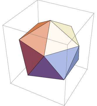
Figura 1: Icosahedron

Having seen how a very small orbit performs, I turn to a maximally large orbit, taking a lattice with 120 vertices. I choose the Great Rhombicosidodecahedron of Figure 2 for this purpose. Each vertex, $X$, lies at the intersection of the spherical bisectors of the spherical triangles making up the fundamental region. The fundamental region can be constructed by adding the face centers and edge centers to the Icosahedral spherical tessellation. Any spherical triangle with 3 vertices in the same triangular Icosahedral face, consisting of one face vertex, one center vertex and one edge center, makes up a fundamental region. The Icosahedron has 20 faces and each has 6 fundamental regions. Therefore there are 120 X-type vertices. If connected by segments of great circles perpendicular to the edges of the fundamental regions, all segments are of equal length. For gaining some familiarity with these constructions I recommend cromwell . A glance at Figure 2 shows that the vertices are not distributed in a very uniform manner. It remains to be seen to what extent this impression correctly reflects on the usefulness of this lattice.

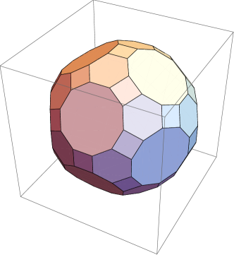
Figura 2: Great Rhombicosidodecahedron

In this case the representation of $I_{h}$ is the regular one, that is, each of the 10 irreducible representations enters into the decomposition a number of times equal to its dimension. Looking at the eigenvalues $\lambda_{k}$ as before, I can go higher up in level. For the $l$-levels that split under $I_{h}$ I take an average over the various $I_{h}$ irreducible representations that contribute, weighted by their sizes. This gives me numbers to compare to the $l(l+1)$ values. I also take the spread of the $\lambda_{k}$ making up the contributions as a measure of the split, $S_{l}$. In this way I found: $\lambda_{l=0}=0$, $\lambda_{l=1}=2$, $\lambda_{l=2}=5.9999$, $\lambda_{l=3}=12.0466$, $\lambda_{l=4}=20.1072$, $\lambda_{l=5}=30.2122$, $\lambda_{l=6}=42.8426$, with $S_{l}=0$ for $l=0,1,2$ and $S_{3}=0.7507$, $S_{4}=0.6882$, $S_{5}=1.3273,1.0562$, $S_{6}=9.2407,9.0609$. Where two numbers appear, I took various combinations of the multiplets into which the particular $l$ decomposed to get some feel. Looking at $l=6$ it is clear that the level identification looses meaning after $l=5$. Nevertheless, even for $l=6$, the average number is close to $l(l+1)$. Multiplicities are always $2l+1$. Looking at the $l=3$ case, we see a much better match with the expected value of $12$ then before. The weighted average is much closer to the expected value than the split would indicate. This looks like an effect of symmetry breaking dominated by a term in an expansion at first order. Perhaps the split of the level $l=3$ seen in  ourplb is of similar origin. That is, in the continuum limit the eigenvalues associated with the icosahedral arrangement of conic singularities in an otherwise flat manifold differs from the spherical, fully rotationally symmetric essentially by a first order perturbation in a symmetry breaking term. This term ought to be predominantly proportional to the primitive $I_{h}$-invariant of order 6.

So far I have only looked at single orbits where the weight is fixed to be the inverse of the orbit size. It is obvious that beyond $l=2$, as expected, splits will occur and that they have a structure that looks perturbative.

More precisely, if I imagined writing a continuum “effective theory” description of the discrete approximation, the continuum $K$ would have corrections which would be still continuum kernels, but break $O(3)$ to $I_{h}$. I could order these corrections by looking at the action restricted to field sectors spanned by low $l$ spherical degrees. The leading correction would be one that becomes felt at the lowest $l$. The corrections, when sandwiched between the states with lowest $l$’s which are going to split must generate an invariant under $I_{h}$ which is not an invariant under $O(3)$. The lowest degree of that integrand is 6, as already discussed. The affected $l$’s of the fields would than have to be, as expected, $l=3$. There is only one parameter that enters, associated with the degree 6 invariant. To leading order the effect cancels out in the multiplicity weighted average. That makes the deviation of $\lambda_{l=3}$ from 12 quite small. At $l=5$ the degree 10 invariant enters and a larger split occurs, reflecting the extra coupling. I plan to report separately on a more detailed analysis of these breaking effects future1 .

Now I wish to look at a minimal example in which I have two orbits, and, by adjusting their weights I can eliminate the split in the $l=3$ level. I take the Icosahedron and add to it the centers of the faces. This gives me in total 32 vertices and 2 orbits. There is one free parameter, which is the ratio of the two weights. See Figure 3. I want to use it in order to zero out the split. At the level of cubature this is a well known problem, solved long ago sobolev . I require that the weights be such that at the level of simple cubature, where the action density (not the fields) is expanded in spherical harmonics, there be exact agreement between the sum and integral for $l=6$. In fact, I am zeroing out the coupling of the degree 6 invariant. As explained before, this ensures sum and integral agreement of the simple cubature formula all the way up to $l=9$. If $s$ is large enough, as I explained, one expects no breaking effects up to and including level $l=4$. That is, both the splits of $l=3$ and $l=4$ should be small.

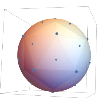
Figura 3: A 32 vertex, 2 orbits arrangement.

Picking the weights $w_{c}=\frac{f}{20(1+f)}$ and $w_{v}=\frac{1}{12(1+f)}$ for the orbit of triangle centers and that of original vertices respectively, and using $f=1.8$, the exact value derived from the simple cubature equation, I obtained, again with $s=0.7$, $\lambda_{0}=1$, $\lambda_{1}=2$, $\lambda_{2}=6$, $\lambda_{3}=12$, $\lambda_{4}=20$ with increasing deviations as $l$ increases. The largest deviations are of order $10^{-7}$, which is the order of the split at $l=4$. As $s$ is increased the splits drop dramatically even further, in accordance with our analysis earlier. At $l=5$ the structure has totally deteriorated: indeed up to $l=4$, 25 states were accounted for. The $l=5$ state would add 11 states, but we only have 32-25=7 left. These 7 states come in two triplets and a singlet.

The findings so far support the approach, but only at the level of the quadratic part of the action, which, from the point of view of field theory corresponds to free field theory. I need to get some feel for the situation in an interacting situation.

V.2 Large N

Consider the CFT generated by the continuum linear or nonlinear $O(N)$ model in three Euclidean dimensions. It is well known that at leading order in $1/N$ the model can be described by a free massless field theory for $N$ scalar fields. One needs to adjust one coupling to make the theory massless, and like any free massless scalar theory it is also a CFT.

The radially quantization of massless scalar fields and the role of conformal invariance were exposed in jackiw . jackiw derives the radially quantized version of the field theory from the same model traditionally quantized on flat two dimensional subspaces of $R^{3}$. In addition to changing variables the correct cylinder structure $R\times S_{2}$ will hold for the case that the scalar fields are rescaled by the appropriate power of the radius. In three dimensions this has the effect of replacing $l(l+1)$ by $l(l+1)+1/4=(l+1/2)^{2}$. The dimensions come from taking square roots of this factor. The 1/4 is crucial in order to get infinite equally spaced towers in the spectrum. In his paper, Cardy cardy , also deals with the $O(N)$ model and shows that the extra $1/4$ is equivalent to the condition for criticality in flat space, obtained by solving the gap equation for the massless case. He does this by endowing the sphere with a radius $R$, and matching to flat space at large $R$. Another way to get the 1/4 is to postulate conformal coupling of the scalar to the round metric on the two-sphere.

In any case, we see in this example explicitly how the flat space adjustment needed for criticality is equivalent to the requirement of having states in the odd $Z_{2}$ sector organize themselves into equally spaced towers.

Working out the explicit CFT structure to higher orders in $1/N$ rapidly becomes a complicated problem ruhl .

In ourplb we showed that in two dimension the $O(N)$ model does not admit an adjustment which would make the towers equally spaced. This is consistent with the model having to break scaling at the quantum level.

V.3 A transfer matrix example

So far I have checked that the construction of an action thinking in terms of cubature formulas has a chance to work. Quantum mechanically however, all that was checked was free field theory.

Now I want to work out one example which is fully interacting. I want an example that I can do almost analytically. By this I mean that I can, in a matter of a few minutes on the computer, get very high accuracy results without using anything stochastic.

The example consists of the Ising model defined on the sphere with 12 Icosahedral vertices. The associated transfer matrix is $2^{12}\times 2^{12}$ and can be fully diagonalized with standard routines. I am forced to use the Ising model in order to minimize the number of values the fields can take, while still having a global internal $Z_{2}$ symmetry.

Since the heat kernel formalism has been checked already, I am not bound to it. I only adopt the idea to use a non-local interaction and am going to adjust it the best I can.

It is well known that the Ising model can be written in terms of continuum fields zinn . This makes the application of mean field theory straightforward. I do not need the explicit expressions. The main point is that there is a quadratic kernel whose eigenvalues and behaviour under rotations are still relevant although the original fields were discretely valued. However, the potential is not polynomial and therefore the symmetry analysis I presented before does not apply. There are also other problems, making a transfer matrix in terms of the continuous fields untenable.

The strategy is as follows: first treat the quadratic part as if this was a free theory with a continuously valued real scalar field. Adjust in such a manner that it give the best rendition of the spherical Laplacian possible. Then use it to define the spin-spin interaction in the Ising model. The hope is that this structure would ensure that one can find a large region of parameter space where the order of low states is what one expects from the model. Next, introduce two more couplings, and search for a pseudo critical point. This point is characterized by some CFT spectral regularity holding there at a reasonable level of accuracy. The criterion is that spacings between the two lowest rungs in tentatively identified towers agree between the odd and even sector. I also require to tentatively identify the state corresponding to the energy momentum tensor. If all three independent determinations of scale agree with other, I can get rough numbers for the dimensions of some of the lowest primaries. The main intention is to see the right structure and numbers in the right ballpark. It would be unrealistic to expect more from such a small system. I diagonalize the transfer matrix to get its spectrum and symmetry properties of the lowest states.

V.3.1 The spin-spin interaction

On each site of one spherical shell we have a spin $\sigma_{i}=\pm 1$. The sites are labelled by 1 to 12. The labels, according to the Icosahedral net in Figure 4 go as follows: the top row are all site 1. The next horizontal row has labels 2,3,4,5,6,2 left to right, followed by labels 7,8,9,10,11,7 and the bottom row are all site 12.

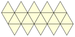
Figura 4: Icosahedral Net

The term in the action I am now focusing on is

$${\cal A}=\sum_{i\neq j}\sigma_{i}C_{i,j}\sigma_{j}$$ (21)

My objective is to determine the off diagonal entries in the symmetric matrix $C_{i,j}$. I do not want this choice, in itself, to violate $O(3)$. So, $C_{i,j}$ only depends on $\hat{\omega}_{i}\cdot\hat{\omega}_{j}$. The distances between non-identical sites take only three values. If I only made $C_{i,j}\neq 0$ zero for the shortest non-zero distance, there would be no indication that the sites reside on a sphere rather than on the corners of a solid Icosahedron. The 12 dimensional representation of $I_{h}$ provided by this set of sites decomposes into $A_{g}\oplus F_{1u}\oplus F_{2u}\oplus H_{g}$, as already mentioned. I can introduce 3 different parameters corresponding to the 3 values of distances; they correspond to the 3 non-trivial irreducible representations above.

With the above labelling the most general $C_{i,j}$ $O(3)$-invariant matrix is

$$C=\left({\scriptscriptstyle\begin{array}[]{cccccccccccc}0&a&a&a&a&a&b&b&b&b&b&c\\ a&0&a&b&b&a&a&b&c&b&a&b\\ a&a&0&a&b&b&a&a&b&c&b&b\\ a&b&a&0&a&b&b&a&a&b&c&b\\ a&b&b&a&0&a&c&b&a&a&b&b\\ a&a&b&b&a&0&b&c&b&a&a&b\\ b&a&a&b&c&b&0&a&b&b&a&a\\ b&b&a&a&b&c&a&0&a&b&b&a\\ b&c&b&a&a&b&b&a&0&a&b&a\\ b&b&c&b&a&a&b&b&a&0&a&a\\ b&a&b&c&b&a&a&b&b&a&0&a\\ c&b&b&b&b&b&a&a&a&a&a&0\\ \end{array}}\right)$$ (22)

One has

$$C=aX+bY+cZ,$$ (23)

and the matrices $X,Y,Z$ commute.

Using the explicit labelling it is easy to verify that the permutation matrix $Z$ is the inversion.

$$Z=\left({\scriptscriptstyle\begin{array}[]{cccccccccccc}1&0&0&0&0&0&0&0&0&0&0&0\\ 0&0&1&0&0&0&0&0&0&0&0&0\\ 0&0&0&1&0&0&0&0&0&0&0&0\\ 0&0&0&0&1&0&0&0&0&0&0&0\\ 0&0&0&0&0&1&0&0&0&0&0&0\\ 0&1&0&0&0&0&0&0&0&0&0&0\\ 0&0&0&0&0&0&0&1&0&0&0&0\\ 0&0&0&0&0&0&0&0&1&0&0&0\\ 0&0&0&0&0&0&0&0&0&1&0&0\\ 0&0&0&0&0&0&0&0&0&0&1&0\\ 0&0&0&0&0&0&1&0&0&0&0&0\\ 0&0&0&0&0&0&0&0&0&0&0&1\\ \end{array}}\right)$$ (24)

Projecting on the two subspaces invariant under $Z$, $X$ decomposes as $X=X_{1}+X_{2}$ and $Y$ decomposes as $Y=Y_{1}+Y_{2}$. It is easy to check that $X_{1}=Y_{1},X_{2}=-Y_{2}$. Hence we can choose $X_{1},X_{2},Z$ as the complete set of commuting operators for this problem.

Both $X_{1}$ and $X_{2}$ have 6 dimensional kernels. The non-zero spectrum of $X_{1}$ consists of $5$ (singlet) and $-1$ (quintuplet). The corresponding states are +1 eigenvectors of $Z$. The non-zero spectrum of $X_{2}$ consists of $\pm\sqrt{5}$, two triplets. The corresponding states are -1 eigenvectors of $Z$. So, from $X_{1}$ we have identified the states in $A_{g}\oplus H_{g}$ and from $X_{2}$ the states in $F_{1u}\oplus F_{2u}$. In order to identify which of the $\pm\sqrt{5}$ triplets is $F_{1u}$ and which is $F_{2u}$ we need to look at the action of a rotation by $72^{\circ}$ about an axis of symmetry of the Icosahedron. For the axis connecting the top to bottom vertices in Fig. 4 the action leaves fixed vertex 1 and vertex 12 and cyclically permutes by one step the two remaining horizontal rows simultaneously. The corresponding matrix, $G$ is

$$G=\left(\begin{array}[]{cccccccccccc}1&0&0&0&0&0&0&0&0&0&0&0\\ 0&0&1&0&0&0&0&0&0&0&0&0\\ 0&0&0&1&0&0&0&0&0&0&0&0\\ 0&0&0&0&1&0&0&0&0&0&0&0\\ 0&0&0&0&0&1&0&0&0&0&0&0\\ 0&1&0&0&0&0&0&0&0&0&0&0\\ 0&0&0&0&0&0&0&1&0&0&0&0\\ 0&0&0&0&0&0&0&0&1&0&0&0\\ 0&0&0&0&0&0&0&0&0&1&0&0\\ 0&0&0&0&0&0&0&0&0&0&1&0\\ 0&0&0&0&0&0&1&0&0&0&0&0\\ 0&0&0&0&0&0&0&0&0&0&0&1\\ \end{array}\right).$$ (25)

Now, using the character table and the matrices $G$ and $G^{2}$, one determines that the $\sqrt{5}$ eigenvalue corresponds to $F_{1u}$ and the $-\sqrt{5}$ eigenvalue corresponds to $F_{2u}$. Hence the $-\sqrt{5}$ $X_{2}$ eigenspace should be thought of as descending from $l=3$.

The spectrum of $C$ is linear in the parameters $a,b,c$ and we know now to which continuum $l$ each invariant space should be assigned. It is convenient to add a new variable, $x$, which provides an overall shift of the spectrum of $C$. Now, we have just enough freedom to ensure that the spectrum of the matrix provides eigenvalues associated with $l=3,2,1,0$ given by $-l(l+1)$ in ascending order $-12,-6,-2,0$. I end up with

$$C=-6\;{\mathbb{I}}+\tau X+(1-\tau)Y+Z,$$ (26)

which has a spectrum as close as possible to the continuum Laplacian. Here $\tau=\frac{1+\sqrt{5}}{2}$, the golden ratio. This equation would be directly relevant to continuously valued fields. In the Ising case the contribution of the identity matrix is irrelevant. One will have to rescale the matrix $C$ by a coupling $\beta_{x}$. Because of the relationship to an action in terms of a continuum field I already mentioned, all one can expect is to get the right order and relative magnitudes of eigenvalues. In other words, an overall scale for the energies will have to be determined from the results. This is something one expects. The purpose of the entire exercise is to find a form of the spin-spin interaction that has some likelihood of producing at least the right ordering of states in the discretized version. Here “right” is with respect to the group theoretical identification of the various multiplets with their continuum “parents”.

V.3.2 The spectrum of the transfer matrix

The transfer matrix acts on a 4096 dimensional Hilbert space. A distinct fixed time slice spin configuration $\{s_{j}\}$ labels each element in a basis. The numbering is the same as above, based on the Icosahedral net. The spins $\sigma_{j}$ are given by $\sigma_{j}=2s_{j}-3$, so $s_{j}=1,2$. Any basis element can be labelled by $J=s_{1}+\sum_{j=2}^{12}(s_{j}-1)2^{j-1}$, where $J=1,...,4096$. The spin at vertex $i$ in configuration $J$ is denoted by $\sigma_{i}(J)$. The inverse map is denoted by $J(\{\sigma_{i}\})$.

I define diagonal matrices ${\cal D}$:

$${\cal D}_{J,K}=e^{\frac{1}{2}\beta_{x}\sum_{1\leq i\neq j\leq 12}\sigma_{i}(J)C_{i,j}\sigma_{j}(K)}\delta_{J,K},$$ (27)

with $C$ given by eq. (26). The transfer matrix is given by:

$${\cal T}_{J,K}={\cal D}_{J,J}e^{\beta_{t}\sum_{i=1}^{12}\sigma_{i}(J)\sigma_{i}(K)}{\cal D}_{K,K}.$$ (28)

The internal global $Z_{2}$ symmetry acts by $\sigma_{i}\rightarrow-\sigma_{i},\;\forall i$, which defines the action on the configurations $J,K..\;$. Viewing the $(s_{i}-1)$ as bits, the action is by two’s complement on the integer labelling the configuration. Symmetrizing and anti-symmetrizing ${\cal T}$ with respect to this $Z_{2}$ gives 2 matrices of size $2048\times 2048$ each, ${\cal T}^{A}$ and ${\cal T}^{S}$ . Similarly, the action of the inversion $Z$ can be mapped into an action on the labels $I,J..\;$. I can then decompose ${\cal T}^{A}$ and ${\cal T}^{S}$ separately by projecting on $\pm 1$ eigenspaces of inversion.

Next the four $2048\times 2048$ matrices are numerically diagonalized. That takes little time. I collect the highest eigenvalues of all four matrices. I then know multiplicities, the internal $Z_{2}$ sector and whether the states switch sign under inversion or not. It is not necessary to calculate the eigenvectors for this.

By analogy with ourplb , I have set $\beta_{x}=0.160$ and varied $\beta_{t}$ in the search for a roughly consistent scale determination. I now present a “good” case as far as I can tell after searching not very exhaustively. The logarithm of the highest state energy is 9.8907388587432123. This state is the vacuum. It resides in the even sector where it belongs. I shall subtract from it the logarithms of all the lower energy states. These are the excitation energies. Up to a common rescaling they should provide dimensions of primaries and descendants. Below are numerical results and tentative interpretations of states for $\beta_{t}=0.225$. I use standard notation for the states.

Sect.	Mult.	Excitation Energy
Even	1	1.3142776638306035
Even	3	2.1649446841074473
Even	5	2.3932548321963418
Even	5	2.7868410430944044
Even	4	2.8973684611035200
Even	3	2.9092189893100091
Even	5	3.0638226605671877
Even	1	3.1255791565017601
Even	4	3.5269178230913276

Sect.	Symbol	$l$	Energy
Even	$\epsilon$	0	1.3142776638306035
Even	$\epsilon$	1	2.1649446841074473
Even	$T_{\mu\nu}$	2	2.3932548321963418
Even	$\epsilon$	2	2.7868410430944044
Even	skip 12 states
Even	$\epsilon^{\prime}$	0	3.1255791565017601

Sect.	Mult.	Excitation Energy
Odd	1	0.42744457201564146
Odd	3	1.2689723266444659
Odd	5	1.9039503886862708
Odd	3	2.3895288048861216
Odd	1	2.4721280980424005
Odd	3	3.2980151032493685
Odd	5	3.5915520069173139
Odd	4	3.6018838120548367
Odd	3	3.7001232625160938
Odd	5	3.7286936205459451

Sect	Symbol	$l$	Energy
Odd	$\sigma$	0	0.42744457201564146
Odd	$\sigma$	1	1.2689723266444659
Odd	$\sigma$	2	1.9039503886862708
Odd	$\sigma$	3 ($F_{1u}$)	2.3895288048861216
Odd	$\sigma^{\prime}$	0	2.4721280980424005

Determining the scale from the spacings of the lowest tower members in the even and odd sector I get $\rho=1.182(6)$ and this produces the following dimensions after division by $\rho$: $\dim(\epsilon)=1.553$, $\dim(\epsilon^{\prime})=3.694$, $\dim(T_{\mu\nu})=2.829$, $\dim(\sigma)=0.505$ and $\dim(\sigma^{\prime})=2.922$. I cannot make any serious claims about the validity (to say nothing about the accuracy) of these numbers. My point is that they are in the right ball park. There are serious numerical estimates in the literature to compare to vicari : $\dim(\epsilon)=1.41$, $\dim(\epsilon^{\prime})=3.8$, $\dim(T_{\mu\nu})=3$, $\dim(\sigma)=0.518$, $\dim(\sigma^{\prime})\sim 4.5$. It is encouraging to see that the energy momentum tensor dimension comes out quite close to 3. One also sees how the breakup of higher $l$ multiplets mixes up the order of states pretty early. It would be unrealistic to expect anything more from a spherical shell approximated by just 12 points.

VI Summary

This paper has led me to a quite flexible procedure to set up a Monte Carlo simulation of the radially quantized $\phi^{4}$ model in three dimensions. I have sketched how an analysis would have to be executed. Quite a few details have been left open and adjustments would need to be done as more experience is being accumulated. In broad lines, the procedure is

• Define a sequence of spherical lattices with a convenient decomposition into orbits.

• Determine a set of weights, one per orbit, all positive, such that splits of $l$-mulitplets in the kinetic energy quadratic form are eliminated to a highest possible level $l=l_{\max}$.

• Define the action of a $\phi^{4}\leavevmode\nobreak\ 3\,d$ theory using the weights and the heat kernel kinetic energy.

• Experiment with the choice of $s$ and various approximations to the heat kernel function.

• Make initial Monte Carlo runs to locate consistent level spacings, once it is determined that the actual multiplets hold together well (small splits for a number of $l$’s increasing with the number of orbits). Eliminating splits in the quadratic form of the kinetic energy will not exactly eliminate splits among the actual eigenstates of the transfer matrix, as inferred from various two point correlations.

• Carry out simulations and extract correlation functions.

• Analyze results in an attempt to identify states.

Once reasonable numbers are obtained, with the accumulated experience one can return to the most interesting problem, that is to construct an explicit example of a RG transformation restoring translational invariance at its fixed point and clarify what type of tuning is necessary to induce the flow in the IR to the Wilson-Fisher fixed point.

Even if a good analogue of a Wilsonian RG is not found, the desired continuum limit is still likely to emerge on the basis of results obtained so far. In lieu of a good RG analogue, the classification of corrections subleading in $N$, the number of vertices on one spherical shell, needs to be addressed directly. The natural guess is that the asymptotics as $N\to\infty$ can be expressed by an effective continuum action whose leading term alone produces the continuum radially quantized target CFT and corrections are ordered by dimensions of scalar primaries. This can hold only up to some non-zero fraction of $N$, $\zeta N$. The states with dimensions lower than $\zeta N$ fall into angular momentum multiplets which stay unsplit under $I_{h}$. The assumption is that $\zeta$ stays larger than zero as $N\to\infty$.

At this point it is premature to present generalizations of lattice radial quantization to non-scalar fields future1 .

- (1) R. C. Brower, G. F. Fleming, H. Neuberger, Phys. Lett. B 721 (2013) 299.
- (2) J. L. Cardy, J. Phys. A 18 (1985) L757.
- (3) K. I. Macrae, Phys. Rev. D. 23 (1981) 886; N. H. Christ, R. Friedberg, T. D. Lee, Nucl. Phys. B202 (1982) 89.
- (4) G. Strang, G. J. Fix, “An Analysis of the Finite Element Method”, Prentice-Hal, 1973.
- (5) R. C. Brower, M. Cheng and G. T. Fleming, PoS LATTICE 2013, 335.
- (6) R. C. Brower, Talk delivered at the 32nd International Symposium on Lattice Field Theory, 23-28 June, 2014, Columbia University New York, NY.
- (7) J. Cheeger, W. Müller, R. Schrader, Comm. Math Phys. 92 (1984) 405.
- (8) K. Hildebrandt, K. Pothier, M. Wardetzky, Geom. Dedicata 123 (2006) 89.
- (9) R. Sorkin, J. of Math. Phys. (1975) 2432.
- (10) G. R. Stuhne, W. R. Peltier, J. of Comp. Phys. 1948 (1999) 23.
- (11) M. K. Chung, K. J. Worsley, S. Robbins, A. C. Evans, in IEEE, “Conference on Computer Vision and Pattern Recognition (CVPR)”, vol I (2003) 467.
- (12) K. Binder, Z. Phys. B 43 (1981) 119.
- (13) A. Pelissetto, E. Vicari, Phys. Rept. 368 (2002) 549.
- (14) M. Weigel, W. Janke, Phys. A 281 (2000) 287.
- (15) B. S. Kay, U. M. Studer, Comm. Math. Phys. 139 (1991) 103.
- (16) V. Frolov, D. Fursaev, Class., Qu., Grav. 18 (2001) 1535.
- (17) K. Atkinson, W. Han, “Spherical Harmonics and Approximations on the Unit Sphere: An Introduction”, Springer 2012.
- (18) R. Narayanan, H. Neuberger, JHEP 0603, 064 (2006).
- (19) C. Ahrens, G. Beylkin, Proc. R. Soc. A 465 (2009) 3103; N. L. Fernández, Elec. Trans. on Num. Anal. 19 (2005) 84; J. Prestin, D. Roşca, J. of Approx. Th. 142 (2006) 1.
- (20) G. Benfatto, G. Gallavotti, “Renormalization Group”, Princeton University Press (1995).
- (21) M. Belkin, P. Niyogi, Neural Computation 15 (2003) 1373.
- (22) G. Dziuk, “Finite elements for the Beltrami operator on arbitrary surfaces”. In “Partial Differential Equations and Calculus of Variations”, S. Hildebrandt and R. Leis, eds., Vol 13, Lecture Notes in Mathematics, Springer (1988) 142; G. Dziuk, C. M. Elliott, Acta Numerica (2013) 289.
- (23) H. Neuberger, Phys. Lett. B417 (1998) 141.
- (24) S. Minakshisundaram, . Pleijel, Can. J. Math. I (1949) 242.
- (25) A. Jaffe and G. Ritter, Commun. Math. Phys. 270 (2007) 545; arXiv:0704.0052 [hep-th].
- (26) E. S. Hsu, “Stochastic Analysis on Manifolds”, AMS (2001).
- (27) M. S. Dresselhaus, G. Dresselhaus, A. Jorio, “Group Theory, Application to the Physics of Condensed Matter”, Springer (2008).
- (28) N. B. Backhouse, P. Gard, J. Phys. A: Math. Nucl. Gen. 7 (1974) 2101.
- (29) S. L. Sobolev, Dokl. Akad. Nauk SSSR 146 (1962) 41, Dokl. Akad. Nauk SSSR 146 (1962) 310, Dokl. Akad. Nauk SSSR 146 (1962) 770; J. M. Goethals, J. J. Seidel, “Cubature Formulae, Polytopes, and Spherical Designs”, in “The Geometric Vein”, C. Davis et. al. (eds), Springer-Verlag, NY, 1981.
- (30) L. Flatto, Bull. Amer. Math. Soc., 74 (1968) 730.
- (31) H. S. M. Coxeter, “Regular Polytopes”, Dover (1973).
- (32) J. E. Humphreys, “Reflection Groups and Coxeter Groups”, Cambridge University Press (1990).
- (33) F. Klein, “Vorlesungen über das Ikosaeder und die Auflösung der Gleichungen fünften Grades”, Leipzig (1884).
- (34) H. Neuberger, Phys. Lett. B 199 (1987) 536; U. M. Heller, M. Klomfass, H. Neuberger and P. M. Vranas, Nucl. Phys. B 405 (1993) 555.
- (35) P. R. Cromwell, “Polyhedra”, Cambridge University Press (1997).
- (36) H. Neuberger, in preparation.
- (37) S. Fubini, A. J. Hanson, R. Jackiw, Phys. Rev. D 7 (1973) 1732.
- (38) K. Lang, W. Rühl, Nucl. Phys. B402 (1993) 573.
- (39) J. Zinn-Justin, “Quantum Field Theory and Critical Phenomena”, Oxford University Press (1999).