The charge-asymmetric nonlocally-determined local-electric (CANDLE) solvation model

Abstract

Many important applications of electronic structure methods involve molecules or solid surfaces in a solvent medium. Since explicit treatment of the solvent in such methods is usually not practical, calculations often employ continuum solvation models to approximate the effect of the solvent. Previous solvation models either involve a parametrization based on atomic radii, which limits the class of applicable solutes, or based on solute electron density, which is more general but less accurate, especially for charged systems. We develop an accurate and general solvation model that includes a cavity that is a nonlocal functional of both solute electron density and potential, local dielectric response on this nonlocally-determined cavity, and nonlocal approximations to the cavity-formation and dispersion energies. The dependence of the cavity on the solute potential enables an explicit treatment of the solvent charge asymmetry. With only three parameters per solvent, this ‘CANDLE’ model simultaneously reproduces solvation energies of large datasets of neutral molecules, cations and anions with a mean absolute error of 1.8 kcal/mol in water and 3.0 kcal/mol in acetonitrile.

I Introduction

Solvents play a critical role in determining chemical reaction mechanisms and rates, but the need for thermodynamic phase-space sampling renders direct treatment of the liquid in electronic structure calculations far too computationally intensive. The standard solution to this problem is to use continuum solvation models which empirically describe the dominant effects of the solvent within a single electronic structure calculation of the solute alone. This enables rapid estimations of free energies of reaction intermediates, allowing for a theoretical screening of reaction mechanisms, and providing insight into the mechanisms involved in catalysis required for the development of more efficient catalysts.

Conventional continuum solvation models such as the ‘SM’ series Cramer and Truhlar (1991); Marenich et al. (2007); Marenich, Cramer, and Truhlar (2009) and the polarizable continuum models (PCMs) Fortunelli and Tomasi (1994); Barone, Cossi, and Tomasi (1997); Tomasi, Mennucci, and Cammi (2005) construct cavities composed of a union of van der Waals (vdW) spheres centered on the solute atoms, and approximate the effect of the solvent by the electric response of a continuum dielectric cavity along with empirical corrections for cavity formation and dispersion energies. These models include a number of atom-dependent parameters such as radii and effective atomic surface tensions which are fit to datasets of experimental solvation energies, typically including neutral and charged organic solutes. These models can be quite accurate for the solvation energies of solutes similar to those in the fit set, but require care when extrapolating to new systems. Additionally, the sharp cavities generated from the union of atomic spheres can lead to numerical difficulties including non-analyticities in the energy landscape for ionic motion that complicates geometry optimization and molecular dynamics of the solute.

In contrast, density-based solvation models such as the self-consistent continuum solvation (SCCS) approach Andreussi, Dabo, and Marzari (2012); Dupont, Andreussi, and Marzari (2013) and the simplified solvation models Letchworth-Weaver and Arias (2012); Gunceler et al. (2013); Sundararaman, Gunceler, and Arias (2014) within joint-density functional theory (JDFT) Petrosyan et al. (2007) employ a continuously varying dielectric constant determined from the solute electron density. These models avoid the numerical difficulties arising from sharp spheres making them more naturally suited for the plane-wave basis sets used in solid-state calculations. Additionally, density-based solvation models typically involve fewer (two to four) parameters and should extrapolate more reliably from one class of solute systems to another. However, the smaller parameter set also limits the typical accuracy achievable in this class of models. In particular, these solvation models exhibit a systematic error between the solvation of cations and anions, with cations in water over-solvated and anions under-solvated. This issue is sometimes handled by fitting separate parameter sets for differently-charged solutes,Dupont, Andreussi, and Marzari (2013) but that is not an option for solutes that combine centers of opposite charges such as zwitterions or ionic surfaces.

Here we report a highly accurate density-based solvation model that addresses the aforementioned charge asymmetry issue. We start with the recent non-empirical solvation model, ‘SaLSA’,Sundararaman et al. (2014) derived from the linear-response limit of joint density-functional theory,Petrosyan et al. (2007) which provides an excellent starting point due to the independence of its cavity from fitting to solvation energies, and provides additional numerical stability from the nonlocality in the determination of the cavity, the electric response, cavity formation free energy and dispersion energy. To account for the charge asymmetry, section II.1 introduces a nonlocal dependence of the cavity on both the electron density and electric potential of the solute.

In SaLSA, the nonlocal electric response involves an angular momentum expansion which converges rapidly only for small sphere-like solvent molecules (such as water) and which increases the computational expense by one-two orders of magnitude compared to local response. Section II.2 replaces the nonlocal electric response with a local dielectric as in traditional continuum solvation models, but derived from the nonlocal cavity that builds in the charge asymmetry. Because it is based on the Charge-Asymmetric Nonlocally-Determined Local Electric response, we refer to this new model as the CANDLE solvation model. The treatment of the cavity formation and dispersion energies are almost identical to SaLSA,Sundararaman, Gunceler, and Arias (2014); Sundararaman et al. (2014) except for minor modifications to the dispersion functional (section II.3) to improve the generalization to solvents of highly non-spherical molecules. Finally, section III details the fits of the three parameters in the model – a charge asymmetry parameter, an electric response nonlocality parameter and the dispersion scale factor – to experimental solvation energies. That section then demonstrates the accuracy of the CANDLE solvation model for water and acetonitrile as prototypical solvents.

II Description of model

Following the SaLSA solvation model,Sundararaman et al. (2014) we approximate the total free energy of a solvated electronic system as

$$A_{\textrm{sol}}[n]=A_{\textrm{HK}}[n]+U_{\textrm{lq}}[\rho_{\textrm{el}},s]+G_{\textrm{cav}}[s]+E_{\textrm{disp}}[s].$$ (1)

Here, $A_{\textrm{HK}}[n]$ is the Hohenberg-Kohn functionalHohenberg and Kohn (1964) of the solute electron density $n(\vec{r})$, which in practice we treat using the Kohn-Sham formalismKohn and Sham (1965) with an approximate exchange-correlation functional. The second term $U_{\textrm{lq}}[\rho_{\textrm{el}},s]$ is the electrostatic interaction energy between the solute and solvent, where $\rho_{\textrm{el}}(\vec{r})$ is the total (electronic + nuclear) solute charge density and $s(\vec{r})$ is the cavity shape function which switches smoothly from 0 in the region of space occupied by the solute to 1 in that occupied by the solvent. The third and fourth terms of (1) capture the cavity formation free energy and dispersion energy respectively.

The following sections describe each of the above terms in detail. Section II.1 presents the determination of the cavity shape function $s(\vec{r})$, section II.2 describes the electric response of the solvent that determines $U_{\textrm{lq}}$ and section II.3 details the dispersion energy $E_{\textrm{disp}}$.

For the cavity formation free energy $G_{\textrm{cav}}$, we adopt the parameter-free weighted density approximation from Ref. 11 without modification. Briefly, this model for the cavity formation free energy begins with a weighted-density ansatz motivated from an intuitive microscopic picture of surface tension and completely constrains the functional form to bulk properties of the solvent including the number density, surface tension and vapor pressure. The resulting functional accurately describes the free energy of forming microscopic cavities of arbitrary shape and size in comparison to classical density-functional theory and molecular dynamics results.Sundararaman, Letchworth-Weaver, and Arias (2014) (See Ref. 11 for a full specification of $G_{\textrm{cav}}[s]$.)

II.1 Cavity determination

Traditional density-based solvation models determine the cavity as a local function of the solute electron density, $s(\vec{r})=s(n(\vec{r}))$, that switches from 0 to 1 over some density range (controlled by $n_{c}$ in the JDFT simplified solvation modelsLetchworth-Weaver and Arias (2012); Gunceler et al. (2013) and by $(\rho_{\textrm{min}},\rho_{\textrm{max}})$ in the SCCS modelsAndreussi, Dabo, and Marzari (2012); Dupont, Andreussi, and Marzari (2013)) that is fit to solvation energies. In contrast, the non-empirical SaLSA model determines the cavity from an overlap of the solute and solvent electron densities,

$$s(\vec{r})=\frac{1}{2}\operatorname{erfc}\ln\frac{n_{\textrm{lq}}^{0}(r)\ast n(\vec{r})}{\bar{n}_{c}}$$ (2)

where $n_{\textrm{lq}}^{0}(r)$ is a spherical average of the electron density of a single solvent molecule. The critical density product $\bar{n}_{c}=1.42\times 10^{-3}$ is a universal solvent-independent constant determined from a correlation between convolutions of spherical electron densities of pairs of atoms and their van-der-Waals (vdW) radii. (See Ref. 13 for details.)

We make two modifications to the SaLSA cavity determination. First, the spherically-averaged electron density of the solvent molecule produces the correct cavity sizes for the small approximately-spherical solvent molecules (such as water, chloroform and carbon tetrachloride) for which SaLSA works well. To generalize the approach beyond such solvents, and to simplify the construction of the model so as to not depend on electronic structure calculations of the solvent, we replace the solvent electron density with a simple Gaussian model,

$$n_{\textrm{lq}}^{0}(r) \equiv Z_{\textrm{val}}w_{\textrm{lq}}(r)$$

$$\textrm{with }w_{\textrm{lq}}(r) \equiv\frac{1}{(\sigma_{\textrm{lq}}\sqrt{2\pi})^{3}}\exp\left(\frac{-r^{2}}{2\sigma_{\textrm{lq}}^{2}}\right).$$ (3)

Here, $Z_{\textrm{val}}$ is the number of valence electrons in the solvent molecule and the Gaussian width $\sigma_{\textrm{lq}}$ is selected so that the overlap of the model electron densities of two solvent molecules crosses $\bar{n}_{c}$ at a separation equal to twice the vdW radius $R_{\textrm{vdW}}$ of the solvent. This condition reduces to the transcendental equation in $\sigma_{\textrm{lq}}$,

$$(n_{\textrm{lq}}^{0}\ast n_{\textrm{lq}}^{0})(2R_{\textrm{vdW}})=\frac{Z_{\textrm{val}}^{2}}{(2\sigma_{\textrm{lq}}\sqrt{\pi})^{3}}\exp\left(\frac{-R_{\textrm{vdW}}^{2}}{\sigma_{\textrm{lq}}^{2}}\right)=\bar{n}_{c}.$$ (4)

Consistency of the above condition with the correlation between atom density overlaps and atomic vdW radii,Sundararaman et al. (2014) results in cavities of the appropriate size (corresponding approximately to atomic spheres of radius equal to sum of solute atom and solvent vdW radii).

Second, we modify (2) to account for the charge asymmetry in solvation. Dupont and coworkersDupont, Andreussi, and Marzari (2013) show that their characteristic solute electron density parameters that fit the solvation energies of anions in water is an order of magnitude larger than those that fit solvation energies of cations. Thus they recommend separate parameter sets depending on the charge of the solute. We consider this far too restrictive as it precludes applications to solutes that combine sites with different charges. Therefore we build in a dependence of the cavity on the solute electron potential that effectively adjusts the critical electron density depending on the ‘neighborhood’,

$$s(\vec{r})=\frac{1}{2}\operatorname{erfc}\left[\ln\frac{Z_{\textrm{val}}\bar{n}(\vec{r})}{\bar{n}_{c}}\right.\\ \left.-\operatorname{sign}(p_{\textrm{cav}})f_{\textrm{sat}}\left(\left|p_{\textrm{cav}}\right|\hat{e}_{\nabla\bar{n}}\cdot\nabla\hat{K}\bar{\rho}_{\textrm{el}}(\vec{r})\right)\right].$$ (5)

Here, $\bar{n}\equiv w_{\textrm{lq}}\ast n$ and $\bar{\rho}_{\textrm{el}}\equiv w_{\textrm{lq}}\ast\rho_{\textrm{el}}$ are weighted electron densities and total charge densities respectively. The remainder of this section specifies the remaining attributes of (5).

The combination $\nabla\hat{K}\bar{\rho}_{\textrm{el}}$ is the negative of the electric field due to the solute (spatially-averaged by the convolution with $w_{\textrm{lq}}$) since $\hat{K}$ is the Coulomb operator, and $\hat{e}_{\nabla\bar{n}}$, the unit vector along $\nabla\bar{n}$, is parallel to the inward normal of the cavity. Therefore, the argument of $f_{\textrm{sat}}$ in (5) is proportional to the spatially-averaged outward electric field due to solute, which is negative for cation-like regions and positive for anion-like regions (using an electron-is-positive sign convention for electrostatics).

Now note that we can write (5) as (2) with $\bar{n}_{c}$ replaced with $\bar{n}_{c}^{\textrm{eff}}=\bar{n}_{c}e^{\operatorname{sign}(p_{\textrm{cav}})f_{\textrm{sat}}(x)}$, where $x$ is the combination discussed above that measures the local ‘anion-ness’. The SCCS solvation fits for ions required electron density parameters for anions about an order of magnitude larger than those for cations and neutral molecules.Dupont, Andreussi, and Marzari (2013) We impose the following conditions on $f_{\textrm{sat}}(x)$:

• $f_{\textrm{sat}}(x)=0$ for $x<0$ (cation-like regions) to reproduce the similarity of cation and neutral parameters.

• For $x>0$ (anions), $f_{\textrm{sat}}(x)$ saturates to $D_{\textrm{max}}$ for large $x$ so that the modulation of $\bar{n}_{c}^{\textrm{eff}}$ is limited to a factor of $e^{D_{\textrm{max}}}$. This provides numerical stability. We set $D_{\textrm{max}}=3$ which is just sufficient to cover the parameter changes observed in the SCCS fits.

• $f_{\textrm{sat}}(x)$ is continuous and differentiable.

In order to satisfy these conditions, we select

$$f_{\textrm{sat}}(x)=D_{\textrm{max}}\begin{cases}0,&x\leq 0\\ \tanh x^{2},&x>0.\end{cases}$$ (6)

This parametrization is of course not unique, but it is one of the simplest choices that captures the observed charge asymmetry and remains numerically stable. Note that a similar dependence on the solute electric field would be extremely unstable in a conventional isodensity model that depends on the local electronic density. Here the nonlocality introduced by the convolutions with $w_{\textrm{lq}}(r)$ is critical to the success of the present model.

Finally, the fit parameter $p_{\textrm{cav}}$ selects the sensitivity of the cavity to the solute electric field. Water requires $p_{\textrm{cav}}>0$ because anions in water require a larger $\bar{n}_{c}^{\textrm{eff}}$ than cations. Some solvents, such as acetonitrile, exhibit the opposite asymmetry. Note that we split the sign and magnitude of $p_{\textrm{cav}}$ in the formulation of (5), so that the charge asymmetry correction always applies to anions rather than cations. We could have alternatively applied the correction to anions when $p_{\textrm{cav}}>0$ and to cations when $p_{\textrm{cav}}<0$. However, this choice leads to an instability for cations when $p_{\textrm{cav}}<0$: a decrease in the electron density near the nuclei increases the electric field, reduces the cavity size, increases the solvation of the electrons, and favors a further decrease in electron density. (The similar situation of anions for $p_{\textrm{cav}}>0$ is stable because increases in electron density are limited by the associated Kohn-Sham kinetic energy cost.)

II.2 Electric response

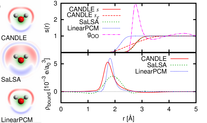
Figure 1: Comparison of the cavity shape functions and bound charges ($\rho_{\textrm{bound}}(\vec{r})$) for a water molecule in water from the CANDLE, SaLSASundararaman et al. (2014) and local LinearPCMGunceler et al. (2013) models. The experimental oxygen-oxygen radial distribution functionSoper (2000) $g_{OO}(r)$ is also shown for comparison. Note that the SaLSA and CANDLE $s(\vec{R})$ are almost superimposed. The left panels show the bound charge ($+$ red, $-$ blue) and electron density (green).

The cavity of conventional density-based solvation models represents the shape of an effective continuum dielectric that reproduces solvation energies. In contrast, the cavity of the SaLSA model (and hence the one determined above) corresponds to the physical distribution of solvent molecule centers because the model directly captures the nonlocal dielectric response of the solvent molecules. However, this nonlocal dielectric response requires an expansion in angular momentum that is computationally intensive and practically applicable only for solvents involving small, approximately spherical and rigid molecules.

The CANDLE solvation model restores the standard local response approximation to achieve computational expediency and generality, but this in turn then requires an empirical description of the dielectric as in other local solvation models. We use the dielectric shape function

$$s_{\epsilon}(\vec{r})=s(\vec{r})\ast\frac{\delta(r-\eta)}{4\pi\eta^{2}},$$ (7)

which extends an empirical distance $\eta$ closer to the solute than the solvent-center cavity $s(\vec{r})$ described by (5). The solvent electric response is then approximated by a continuum dielectric $\epsilon_{b}$, optionally with Debye screening $\kappa^{2}=\frac{4\pi}{T}\sum_{i}N_{i}Z_{i}^{2}$ due to finite bulk concentrations $N_{i}$ of ions of charge $Z_{i}$, modulated by the dielectric shape function. The free energy of interaction of the solute charge density $\rho_{\textrm{el}}(\vec{r})$ with the solvent electric response is

$$U_{\textrm{lq}}[\rho_{\textrm{el}}] =\frac{1}{2}\int d\vec{r}\rho_{\textrm{el}}(\vec{r})\left[\hat{K}_{\epsilon}-\hat{K}\right]\rho_{\textrm{el}}(\vec{r}),\textrm{ where}$$

$$\hat{K}_{\epsilon} \equiv\left[\frac{-\nabla\cdot(1+(\epsilon_{b}-1)s_{\epsilon}(\vec{r}))\nabla+\kappa^{2}s_{\epsilon}(\vec{r})}{4\pi}\right]^{-1}$$ (8)

is the screened Coulomb operator. In practice, $\phi=\hat{K}_{\epsilon}\rho_{\textrm{el}}$ is calculated iteratively by solving the modified Poisson (Helmholtz, if $\kappa^{2}\neq 0$) equation, $\hat{K}_{\epsilon}^{-1}\phi=\rho_{\textrm{el}}$, exactly as in previous solvation models.Gunceler et al. (2013)

Figure 1 compares the bound charges and cavity shape functions of the CANDLE solvation model with previous density-based solvation models, for a water molecule in liquid water. The SaLSA and CANDLE $s(\vec{r})$ are almost identical and the transition is at the physical location of the first peak of the radial distribution function $g_{OO}(r)$. The local LinearPCM requires a cavity that transitions much closer to the solute, while the CANDLE $s_{\epsilon}(\vec{r})$ reaches inwards towards the solute with a much wider transition region. The bound charge in the CANDLE solvation model is qualitatively similar to the purely local model, except for a longer tail away from the solute due to the slower variation of the dielectric constant.

II.3 Dispersion energy

Finally, for the dispersion energy, we adopt a slightly modified form of the empirical approximation used in SaLSA,Sundararaman et al. (2014); Sundararaman, Gunceler, and Arias (2014) which applies the DFT-D2 pair potential correctionGrimme (2006) between the discrete solute atoms and a continuous distribution of solvent atoms. The solvent atom distribution is generated from $s(\vec{r})$ by assuming an isotropic orientation distribution of rigid molecules. In order to generalize to non-spherical solvent molecules and eliminate the dependence on the structure of the solvent molecule, we replace the atoms in the solvent molecule with a continuous spherical distribution $w_{\textrm{lq}}(r)$ of local polarizable oscillators with an empirical effective coefficient $C_{\textrm{6eff}}$ each. The resulting simplified dispersion functional is

$$E_{\textrm{disp}}[s]=-\sqrt{C_{\textrm{6eff}}}N_{\textrm{bulk}}\sum_{i}\int d\vec{r}(w_{\textrm{lq}}\ast s)(\vec{r})\\ \times\frac{\sqrt{C_{6i}}}{|\vec{R}_{i}-\vec{r}|^{6}}f_{\textrm{dmp}}\left(\frac{|\vec{R}_{i}-\vec{r}|}{R_{0i}}\right),$$ (9)

where $N_{\textrm{bulk}}$ is the bulk number density of the solvent, $C_{6i}$ and $R_{0i}$ are the DFT-D2 parameters for solute atom $i$ located at position $\vec{R}_{i}$, and $f_{\textrm{dmp}}$ is the short-range damping function (see Refs. 11 and 18 for details). The empirical scale factor $s_{6}$ in the DFT-D2 correction has been absorbed into the empirical $C_{\textrm{6eff}}$ coefficient.

III Results

III.1 Computational details

We implemented the CANDLE solvation model in the open-source plane-wave density functional software, JDFTx.Sundararaman, D. Gunceler, and Arias (2012) The local electric response is evaluated iteratively in the plane-wave basis using exactly the same solver as previous local solvation models,Letchworth-Weaver and Arias (2012); Gunceler et al. (2013) while the nonlocal parts of the functional are shared with or are minor adaptations of the SaLSA model.Sundararaman et al. (2014); Sundararaman, Gunceler, and Arias (2014) The nuclear charge density contributions to $\rho_{\textrm{el}}$ are widened to Gaussians so that they are resolvable on the plane-wave grid (see Ref. 10 for details). In the calculation of the cavity shape function using (5), the valence electron density $n(\vec{r})$ is augmented by $\delta$-functions that account for all the missing core electrons, to be consistent with the all-electron convolutions used in the correlation with vdW radii.Sundararaman et al. (2014)

We perform all calculations with the PBEPerdew, Burke, and Ernzerhof (1996) generalized-gradient approximation to the exchange-correlation functional, and the GBRV ultrasoft pseudopotentialsGarrity et al. (2014) with the recommended wavefunction and charge-density kinetic energy cutoffs of 20 $E_{h}$ and 100 $E_{h}$ respectively. At least 15 $a_{0}$ of vacuum surrounds the solute in each calculation unit cell, and truncated coulomb kernelsMartyna and Tuckerman (1999); Rozzi et al. (2006); Sundararaman and Arias (2013) are used to eliminate the interaction between periodic images.

III.2 Parameter fitting

Parameter	Water	Acetonitrile
Fit:
$p_{\textrm{cav}}$ [$ea_{0}/E_{h}$]	36.5	-31.0
$\eta$ [$a_{0}$]	1.46	3.15
$\sqrt{C_{\textrm{6eff}}}$ $\left[\left(\frac{\textrm{J}\cdot\textrm{nm}^{6}}{\textrm{mol}}\right)^{1/2}\right]$	0.770	2.21
Physical:
Valence electron count, $Z_{\textrm{val}}$	8	16
vdW radius, $R_{\textrm{vdW}}$ [$\mathring{\textnormal{A}}$]	1.385	2.12
Dielectric constant, $\epsilon_{b}$	78.4	38.8
Bulk density, $N_{\textrm{bulk}}$ [$a_{0}^{-3}$]	$4.938\times 10^{-3}$	$1.709\times 10^{-3}$
Vapor pressure, $p_{\textrm{vap}}$ [kPa]	3.14	11.8
Surface tension, $\sigma_{\textrm{bulk}}$ [$E_{h}/a_{0}^{2}$]	$4.62\times 10^{-5}$	$1.88\times 10^{-5}$

Table 1: Fit parameters and physical properties that constrain the CANDLE solvation model. We obtain vdW radii from Ref. 25 and all other physical properties from Ref. 26 (at standard conditions, $T=298$ K and $p=101.3$ kPa).

The CANDLE solvation model has three parameters per solvent, the charge-asymmetry parameter $p_{\textrm{cav}}$, the electrostatic radius $\eta$ and the effective dispersion parameter $\sqrt{C_{\textrm{6eff}}}$, that are fit to a dataset of experimental solvation energies of neutral molecules, cations and anions in that solvent. Table 1 lists the optimum fit parameters for water and acetonitrile that we determine below, along with values of the physical properties that constrain the solvation model.

We calculate the gas-phase energy for each solute at the optimized vacuum geometry. We optimize the solution-phase geometry using an initial guess for the solvation model parameters, and at that optimum geometry, calculate the solvation energy and its analytical Hellman-Feynman derivatives with respect to the parameters on a coarse grid in the parameter space of the solvation model. Using the analytical derivatives, we interpolate the solvation energies to a finer grid in parameter space and then select the optimum parameters to minimize the mean absolute error (MAE) of all the solutes. We re-optimize the solution-phase geometries with these parameters, and repeat the above parameter sweep process till the optimum parameters converge. For both solvents considered here, the second sweep yields identical optimum parameters as the first, and we show the results of that final self-consistent parameter sweep.

III.3 Water

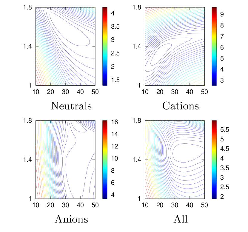
Figure 2: Mean absolute error (MAE) of CANDLE solvation energies of 240 neutral molecules, 51 cations, 55 anions and all of these solutes in water, as a function of the fit parameters. In each panel, the $x$-axis is $p_{\textrm{cav}}$ in $ea_{0}/E_{h}$, the $y$-axis is $\eta$ in $a_{0}$ and the contours (color) axis is MAE in kcal/mol. The $\sqrt{C_{\textrm{6eff}}}$ parameter is set to its optimum value for each combination of the other two parameters.

Using the above protocol, we fit the parameters for water to a dataset of 240 neutral molecules, 51 cations and 55 anions, identical to the one used in fitting the SCCS models.Andreussi, Dabo, and Marzari (2012); Dupont, Andreussi, and Marzari (2013) Figure 2 shows the MAE in the solvation energies as a function of the solvation model parameters. Note the extreme sensitivity of the anion solvation energies to the charge-asymmetry parameter $p_{\textrm{cav}}$ ($x$-axis); the MAE for anions would exceed 15 kcal/mol if $p_{\textrm{cav}}$ is set to zero. The neutral molecules and cations more strongly constrain the electrostatic radius $\eta$ ($y$-axis). Overall, the net MAE of all solutes tightly constrains all the parameters. (The solvation energies depend almost linearly on the dispersion parameter $\sqrt{C_{\textrm{6eff}}}$. To simplify the visualization in Figure 2, we ‘integrate out’ the $\sqrt{C_{\textrm{6eff}}}$ parameter by setting it to its optimum value for each combination of the other parameters.)

Model	MAE [kcal/mol]
	Neutral	Cations	Anions	All
GAUSSIAN ’03	–	4.00	10.2	–
GAUSSIAN ’09	–	11.9	15.0	–
SCCS neutral fit 1	1.20	2.55	17.4	3.41
SCCS neutral fit 2	1.28	2.66	16.9	3.35
SCCS cation fit	–	2.26	–	–
SCCS anion fit	–	–	5.54	–
CANDLE	1.27	2.62	3.46	1.81

Table 2: Mean absolute errors (MAE) of the CANDLE solvation model for water compared to various parametrizations of the SCCS model,Andreussi, Dabo, and Marzari (2012) and IEF-PCMMennucci, Cances, and Tomasi (1997); Scalmani and Frisch (2010) in GAUSSIANFrisch et al. using identical sets of solutes. (SCCS and GAUSSIAN results from Ref. 8.)

Table 2 compares the accuracy of the CANDLE solvation model for water with that of the SCCS models and IEF-PCMMennucci, Cances, and Tomasi (1997); Scalmani and Frisch (2010) in GAUSSIANFrisch et al. on exactly the same set of solutes. The IEF-PCM model exhibits large errors for cations as well as anions, while the SCCS model fit to neutral molecules alone, works reasonably well for cations but systematically undersolvates anions resulting in a large error of 17 kcal/mol. This error is reduced to 5.5 kcal/mol by fitting a separate set of parameters for anions alone. With charge asymmetry built in, the CANDLE solvation model with a single parameter set exhibits comparable accuracy to the individual SCCS models fit to each solute type.

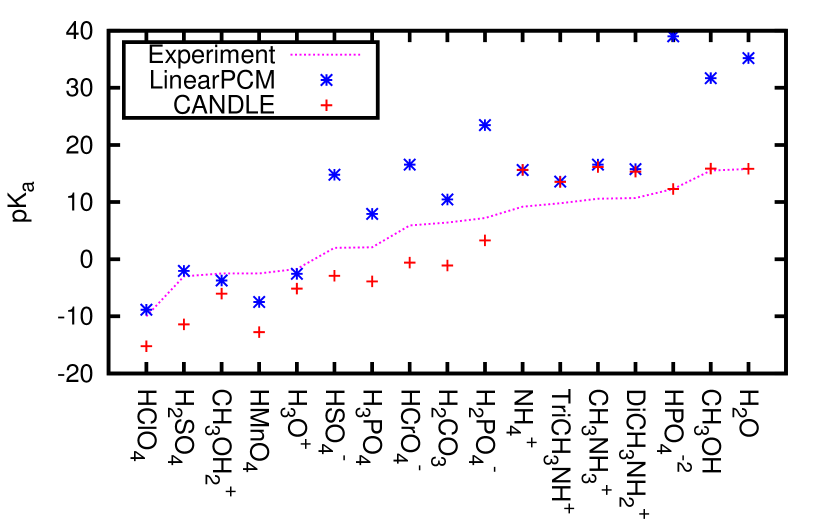
Figure 3: Acid dissociation constants (pKa) in water predicted by the CANDLE and LinearPCMGunceler et al. (2013) models compared to experiment.

As an independent test of accuracy, Figure 3 compares predicted acid dissociation constants of mostly inorganic acids (not present in the fit set) with experiment. The CANDLE model marginally increases the error in pKa of cationic acids compared to the local LinearPCM model, but significantly improves the predictions for neutral and anionic acids since it solves the anion under-solvation issue. Note in particular that CANDLE makes reasonable predictions even for the second and third dissociations of sulfuric and phosphoric acid, which require solvation of dianions and trianions respectively. For the set considered here, the MAE is 4.7 pKa units for CANDLE compared to 8.4 pKa units for LinearPCM.Gunceler et al. (2013)

III.4 Acetonitrile

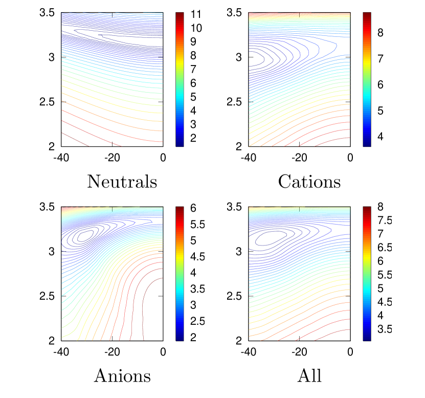
Figure 4: Mean absolute error (MAE) of CANDLE solvation energies of 12 neutral molecules, 30 cations, 39 anions and all of these solutes in acetonitrile, as a function of the fit parameters. The axes are exactly analogous to Figure 2.

For acetonitrile, we fit the CANDLE parameters using the above protocol to the solvation energies of the 12 neutral molecules, 30 cations and 39 anions in the Minnesota solvation database.Marenich et al. (2012) Figure 4 shows the variation of MAE with parameters for the solvation energies in acetonitrile. As in the case of water, the combined set of neutral and charged solutes constrains the fit parameters well. At the optimum parameters, the MAE is 2.35 kcal/mol for neutral molecules, 4.04 kcal/mol for cations, 1.81 kcal/mol for anions, and 2.97 kcal/mol overall.

In contrast to water, the charge asymmetry parameter is negative for acetonitrile indicating that cations are solvated more strongly than anions of the same size. This follows intuitively from the charge distributions of the solvent molecules. In water, the positively-charged hydrogen sites can get closer to the solute than the negatively-charged oxygen and hence anions are solvated more strongly. In acetonitrile, the negatively-charged nitrogen site is more easily solute-accessible whereas the positively-charged carbon site is blocked by the methyl group, and therefore cations are solvated more strongly.

III.5 Solvation of metal surfaces

Finally, we examine the predictions of the CANDLE solvation model for a class of relatively clean electrochemical systems: single crystalline noble metal electrodes in an aqueous non-adsorbing electrolyte. The surface charge on these electrodes depends on the electrochemical potential, and the surface becomes neutral at the potential of zero charge (PZC). Experimentally, these potentials are referenced against the standard hydrogen electrode (SHE). The absolute level of the SHE is difficult to determine experimentally and estimates range from 4.4 to 4.9 eV.Trasatti and Lust (1999) Correlating the theoretical electron chemical potential of solvated neutral metal surfaces with the measured PZC, provides a theoretical estimate of this absolute potential.Letchworth-Weaver and Arias (2012); Gunceler et al. (2013) Here, we reexamine this theoretical estimate with the nonlocal solvation models, CANDLE and SaLSA.

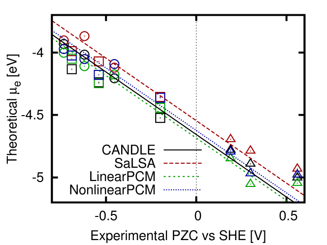
Figure 5: Correlation of theoretical electron chemical potentials ($\mu_{e}$) with experimental potential of zero charge (relative to standard hydrogen electrode (SHE)) for various solvation models. The results are for single crystalline copper (squares), silver (triangles) and gold (circles) surfaces, with 111, 100 and 110 orientations from left to right. (LinearPCM and NonlinearPCM data from Ref. 10.)

Model	$\mu_{\textrm{SHE}}$ [eV]	RMS error [eV]
CANDLE	-4.66	0.11
SaLSA	-4.55	0.09
LinearPCM	-4.68	0.09
NonlinearPCM	-4.62	0.09

Table 3: Offset and RMS deviation between theoretical electron chemical potentials and experimental potentials of zero charge for various solvation models. (LinearPCM and NonlinearPCM data from Ref. 10.)

Figure 5 plots the calculated electron chemical potential of neutral metal surfaces using various solvation models against the experimental PZC, and table 3 summarizes the absolute offset and error in the correlation so obtained. The absolute offsets predicted using various solvation models agree to within 0.1 eV and are well within the expected experimental range. The CANDLE model exhibits a marginally higher scatter, but overall agrees well with the linear and nonlinear local models studied in Ref. 10. The nonlocality of the SaLSA and CANDLE models, therefore, does not significantly alter the predictions of the local solvation models for the absolute SHE potential.

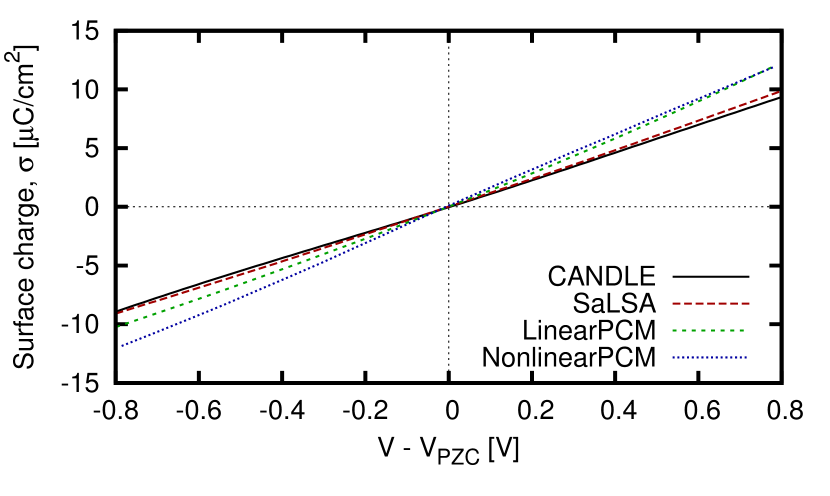
Figure 6: Variation of surface charge on the 111 surface of platinum with electrode potential for various solvation models. (LinearPCM and NonlinearPCM data from Ref. 10.)

The charge of metal electrodes as a function of the electrode potential is sensitive to the structure of the electrochemical double layer and varies nonlinearly, but continuum solvation models predict an almost linear variation (almost constant double layer capacitance).Gunceler et al. (2013) Figure 6 shows that the nonlocal solvation models, CANDLE and SaLSA, also predict a linear charging curve for the Pt 111 surface. The value of the double-layer capacitance is 12 $\mu$F/cm² for these nonlocal models, slightly lower than 14 and 15 $\mu$F/cm² for the linear and nonlinear solvation modelsGunceler et al. (2013) and an experimental estimatePajkossy and Kolb (2001) of $\sim$20 $\mu$F/cm². Details of ion adsorption and the nonlinear capacitance of the electrochemical interface are therefore not described by continuum solvation models and require an explicit treatment of the electrochemical double layer.

IV Conclusions

This work constructs an electron-density-based solvation model, the CANDLE model, that explicitly accounts for the asymmetry in solvation of cations and anions. This model incorporates the charge asymmetry by adjusting the effective electron density threshold parameter (and hence the cavity size) depending on the local charge environment of the solute, which in turn is measured using the direction of the solute electric field on the cavity surface. The CANDLE model exploits the nonlocal cavity determination and approximations to the cavity formation and dispersion energies of the fully nonlocal SaLSA model,Sundararaman et al. (2014) but replaces the nonlocal electric response with an effective local response, thereby combining the computational efficiency of standard local-response solvation models with the stability and accuracy of the nonlocal model.

With just three parameters per solvent, the CANDLE model predicts solvation energies of neutral molecules, cations and anions in water and acetonitrile with higher accuracy than previous density-based solvation models. Since a single set of parameters works for differently charged solutes, the CANDLE model is particularly important for systems that expose strongly-charged positive as well as negative centers to solution, such as ionic surfaces. A comparative study of solvation models for solid-liquid interfaces would be particularly desirable, but difficult due to the dearth of directly calculable experimental properties (analogous to solvation energies for finite systems). Constraining the parameters of this model requires experimental solvation energies for neutral as well as charged solutes, but extensive data is available only for a small number of solvents. The trends in the CANDLE parameters for other solvents for which ion solvation data is available will be useful in estimating the parameters and accuracy of the CANDLE model for solvents without such data.

References

- Cramer and Truhlar (1991) C. J. Cramer and D. G. Truhlar, J.Am. Chem. Soc. 113, 8305 (1991).
- Marenich et al. (2007) A. V. Marenich, R. M. Olson, C. P. Kelly, C. J. Cramer, and D. G. Truhlar, J. Chem. Theory Comput. , 2011 (2007).
- Marenich, Cramer, and Truhlar (2009) A. V. Marenich, C. J. Cramer, and D. G. Truhlar, J. Phys. Chem. B 113, 6378 (2009).
- Fortunelli and Tomasi (1994) A. Fortunelli and J. Tomasi, Chem. Phys. Lett. 231, 34 (1994).
- Barone, Cossi, and Tomasi (1997) V. Barone, M. Cossi, and J. Tomasi, J. Chem. Phys. 107, 3210 (1997).
- Tomasi, Mennucci, and Cammi (2005) J. Tomasi, B. Mennucci, and R. Cammi, Chem. Rev. 105, 2999 (2005).
- Andreussi, Dabo, and Marzari (2012) O. Andreussi, I. Dabo, and N. Marzari, J. Chem. Phys 136, 064102 (2012).
- Dupont, Andreussi, and Marzari (2013) C. Dupont, O. Andreussi, and N. Marzari, J. Chem. Phys 139, 214110 (2013).
- Letchworth-Weaver and Arias (2012) K. Letchworth-Weaver and T. A. Arias, Phys. Rev. B 86, 075140 (2012).
- Gunceler et al. (2013) D. Gunceler, K. Letchworth-Weaver, R. Sundararaman, K. Schwarz, and T. Arias, Modelling Simul. Mater. Sci. Eng. 21, 074005 (2013).
- Sundararaman, Gunceler, and Arias (2014) R. Sundararaman, D. Gunceler, and T. A. Arias, J. Chem. Phys. 141, 134105 (2014).
- Petrosyan et al. (2007) S. A. Petrosyan, J.-F. Briere, D. Roundy, and T. A. Arias, Phys. Rev. B 75, 205105 (2007).
- Sundararaman et al. (2014) R. Sundararaman, K. Schwarz, K. Letchworth-Weaver, and T. A. Arias, “Spicing up continuum solvation models with SaLSA: the spherically-averaged liquid suscpetibility ansatz,” (2014), preprint arXiv:1410.2273.
- Hohenberg and Kohn (1964) P. Hohenberg and W. Kohn, Phys. Rev. 136, B864 (1964).
- Kohn and Sham (1965) W. Kohn and L. Sham, Phys. Rev. 140, A1133 (1965).
- Sundararaman, Letchworth-Weaver, and Arias (2014) R. Sundararaman, K. Letchworth-Weaver, and T. A. Arias, J . Chem. Phys. 140, 144504 (2014).
- Soper (2000) A. K. Soper, Chem. Phys. 258, 121 (2000).
- Grimme (2006) S. Grimme, J. Comput. Chem 27, 1787 (2006).
- Sundararaman, D. Gunceler, and Arias (2012) R. Sundararaman, K. L.-W. D. Gunceler, and T. A. Arias, “JDFTx,” http://jdftx.sourceforge.net (2012).
- Perdew, Burke, and Ernzerhof (1996) J. P. Perdew, K. Burke, and M. Ernzerhof, Phys. Rev. Lett. 77, 3865 (1996).
- Garrity et al. (2014) K. F. Garrity, J. W. Bennett, K. Rabe, and D. Vanderbilt, Comput. Mater. Sci. 81, 446 (2014).
- Martyna and Tuckerman (1999) G. J. Martyna and M. E. Tuckerman, J. Chem. Phys 110, 2810 (1999).
- Rozzi et al. (2006) C. A. Rozzi, D. Varsano, A. Marini, E. K. U. Gross, and A. Rubio, Phys. Rev. B , 205119 (2006).
- Sundararaman and Arias (2013) R. Sundararaman and T. Arias, Phys. Rev. B 87, 165122 (2013).
- Ben-Amotz and Willis (1993) D. Ben-Amotz and K. G. Willis, J. Phys. Chem. 97, 7736 (1993).
- Haynes (2012) W. M. Haynes, ed., CRC Handbook of Physics and Chemistry 93 ed (Taylor and Francis, 2012).
- Mennucci, Cances, and Tomasi (1997) B. Mennucci, E. Cances, and J. Tomasi, J. Phys. Chem. B 101, 10506 (1997).
- Scalmani and Frisch (2010) G. Scalmani and M. J. Frisch, J. Chem. Phys. 132, 114110 (2010).
- (29) M. J. Frisch, G. W. Trucks, H. B. Schlegel, et al., “Gaussian∼09,” Gaussian Inc. Wallingford CT 2009.
- Marenich et al. (2012) A. V. Marenich, C. P. Kelly, J. D. Thompson, G. D. Hawkins, C. C. Chambers, D. J. Giesen, P. Winget, C. J. Cramer, and D. G. Truhlar, Minnesota Solvation Database – version 2012 (University of Minnesota, 2012).
- Trasatti and Lust (1999) S. Trasatti and E. Lust, Modern Aspects of Electrochemistry 33, 1 (1999).
- Pajkossy and Kolb (2001) T. Pajkossy and D. M. Kolb, Electrochimica Acta 46, 3063–3071 (2001).