Generating multipartite entangled states of qubits distributed in different cavities

Abstract

Cavity-based large-scale quantum information processing (QIP) needs a large number of qubits and placing all of them in a single cavity quickly runs into many fundamental and practical problems such as the increase of cavity decay rate and decrease of qubit-cavity coupling strength. Therefore, future QIP most likely will require quantum networks consisting of a large number of cavities, each hosting and coupled to multiple qubits. In this work, we propose a way to prepare a $W$-class entangled state of spatially-separated multiple qubits in different cavities, which are connected to a coupler qubit. Because no cavity photon is excited, decoherence caused by the cavity decay is greatly suppressed during the entanglement preparation. This proposal needs only one coupler qubit and one operational step, and does not require using a classical pulse, so that the engineering complexity is much reduced and the operation is greatly simplified. As an example of the experimental implementation, we further give a numerical analysis, which shows that high-fidelity generation of the $W$ state using three superconducting phase qubits each embedded in a one-dimensional transmission line resonator is feasible within the present circuit QED technique. The proposal is quite general and can be applied to accomplish the same task with other types of qubits such as superconducting flux qubits, charge qubits, quantum dots, nitrogen-vacancy centers and atoms.

I INTRODUCTION

Entanglement is a key resource of quantum information processing (QIP) and quantum communication. During the past decade, a large number of proposals have been presented for entanglement generation. Although most of the quantum information protocols focus on bipartite systems, multipartite entanglement has also attracted much interest because of its potential applications in QIP and quantum communication. It has been shown [1] that there exist two inequivalent classes of multipartite entangled states, i.e., Greenberger-Horne-Zeilinger (GHZ) states [2] and $W$ states [1], which can not be converted to each other by local operations and classical communications. With respect to the tripartite entangled states, it was shown [1] that $W$ states are robust against losses of qubits since they retain bipartite entanglement if we trace out any one qubit, whereas GHZ states are fragile since the remaining bipartite states are separable states. This property turns $W$ states very attractive for various quantum communication tasks. For instances, the $W$ states can be used as quantum channels for teleportation of entangled pairs [3], quantum teleportation [4], quantum key distribution [5] and so on. During the past years, many theoretical schemes for generating $W$ states have been proposed. For examples, (i) schemes have been proposed to generate $W$ states in trapped ions [6,7], atomic ensembles [8], Ising chains with nearest-neighbor coupling by global control [9], or photons on-chip multiport photonic lattices [10]; (ii) by using linear optical elements and photon detection, schemes have been proposed to generate $W$ states of spatially-separated distant atoms [11] or photons [12]; (iii) by using parametric down conversion, schemes have been presented to generate $W$ states of photons [13]; and (iv) based on cavity QED, how to prepare $W$ states has been proposed in quantum dots coupled to a cavity [14], superconducting qubits embedded within a single cavity [15,16], or atoms interacting with a cavity [17,18]. On the other hand, the $W$ states have been experimentally created with up to eight trapped ions [19], four optical modes [20], three superconducting phase qubits coupled capacitively [21], and atomic ensembles in four quantum memories [22], as well as two superconducting phase qubits plus a resonant cavity [23].

The physical system, composed of cavities and qubits, has attracted much attention for QIP. Over the past twenty years, a large number of theoretical and experimental works have been done for implementing quantum information transfer, quantum logical gates, and quantum entanglement with qubits placed inside a single cavity or coupled to a resonator. These works are important in QIP based on cavity QED. However, they are valid only for the case that all qubits are placed in the same cavity or coupled to a common resonator.

Attention is now shifting to large-scale QIP based on cavity QED, which needs a large number of qubits. Note that placing all of qubits in a single cavity quickly runs into many fundamental and practical problems such as the increase of cavity decay rate and decrease of qubit-cavity coupling strength. Therefore, future cavity-based QIP most likely will require quantum networks consisting of a large number of cavities, each hosting and coupled to multiple qubits. In this type of architecture, transfer and exchange of quantum information will not only occur among qubits in the same cavity but also happens between different cavities. Hence, attention must be paid to the preparation of quantum states of two or more cavities, preparation of quantum states of qubits located in different cavities, and implementation of quantum logic gates on qubits distributed over different cavities in a network. All of these ingredients are essential to realizing large-scale QIP based on cavity QED.

Motivated by the above, in this work we focus on how to prepare $W$ states of qubits distributed in many different cavities. Besides its use in large-scale QIP, this work may be also interesting from the following point of view:

The prepared $W$ state can be stored in matter qubits with long decoherence time. Once the $W$ state is needed for quantum communication, one can transfer the $W$ state of matter qubits onto cavity photons and then transmit the cavity photons to distant spatially-separated users located at different nodes in a network. This can be achieved as follows. First, by local operations within every cavity (i.e., a local operation is performed on a qubit and a cavity in which the qubit is placed, so that the state of the qubit is transferred onto the cavity photon), one can transfer the $W$ state of matter qubits onto the cavity photons. Second, to transmit a cavity photon to a distant user in a network, one can increase the cavity-decay rate (e.g., by adjusting the mirrors at the end of an optical cavity or lowering the cavity quality factor for a circuit cavity) to have the cavity photon leaked into an optical fiber, which connects the cavity with the distant user. In this way, the $W$ state of the cavity photons can be shared by different users in a network, and can be used as a quantum channel for carrying out quantum communication tasks.

In the following, we will present a way for preparing $W$ states of qubits distributed in $n$ different cavities. As shown below, this proposal has the following advantages: (i) the entanglement preparation is performed without excitation of the cavity photons, and thus decoherence induced by the cavity decay is greatly suppressed; (ii) only one coupler qubit is needed, one operational step is required, and no classical pulse is used, hence the engineering complex is much reduced and the operation is greatly simplified; and (iii) the operation time decreases as the number of qubits increases.

This proposal is quite general, and can be applied to accomplish the same task with different types of qubits, such as quantum dots, atoms, NV centers, superconducting qubits (e.g., phase, flux and charge qubits), and so on. To the best of our knowledge, how to create the $W$ state of qubits, distributed in different cavities connecting to a coupler qubit, has not been reported so far.

This paper is organized as follows. In Sec. 2, we show how to generate the $W$ state of $n$ qubits distributed in $n$ different cavities. In Sec. 3, as an example, we analyze the experimental feasibility of preparing the $W$ state of three superconducting phase qubits, which are distributed in three different one-dimensional transmission line resonators. A concluding summary is enclosed in Sec. 4.

II W-STATE PREPARATION

In this section, we first construct a Hamiltonian for the $W$ state preparation. We then give a discussion on how to prepare the $W$ state of $n$ qubits $\left(1,2,...,n\right)$ distributed in the $n$ cavities.

II.1 Hamiltonian

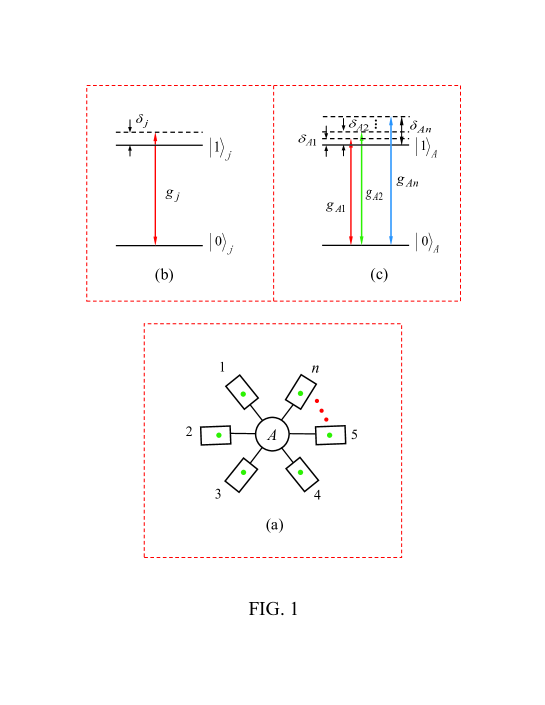
Figure 1: (color online) (a) Diagram of a coupler qubit $A$ (a circle at the center) and $n$ cavities each hosting a qubit. A dark square represents a cavity while a green dot labels a qubit placed in each cavity, which can be an atom or a solid-state qubit. The coupler qubit $A$ can be an atom or a quantum dot, and can also be a superconducting qubit capacitively or inductively coupled to each cavity. (b) Cavity $j$ dispersively coupled to qubit $j$ (placed in cavity $j$) with coupling constant $g_{j}$ and detuning $\delta_{j}$. (c) The coupler qubit $A$ dispersively interacting with $n$ cavities simultaneously, with coupling constant $g_{Aj}$ and detuning $\delta_{Aj}$ for cavity $j$ ($j=1,2,...,n$). Here, $\delta_{Aj}=\delta_{j}$, which holds for identical qubits $A$ and $j$. Note that in (a), only one qubit in each cavity is drawn for simplicity. In reality, for a quantum processor with multiple registers—each register consists of a cavity and qubits in the cavity, more than one qubit are usually placed in each cavity. To prepare the $W$ state of $n$ qubits each in a different cavity, only one qubit in each cavity is involved in the entanglement preparation, while other qubits in each cavity can be made to be decoupled from their cavity by adjusting their level spacings (e.g., solid-state qubits) or by moving them out of their cavity (e.g., atomic qubits), such that they do not participate during the $W$ state preparation.

Consider $n$ cavities $(1,2,...,n)$ connected to a coupler qubit $A$, as illustrated in Fig. 1(a). Cavity $j$ ($j=1,2,...n$) hosts qubit $j$, shown as a black dot. Each qubit here has two levels $\left|0\right\rangle$ and $\left|1\right\rangle.$ Assume that the coupling constant of qubit $j$ with cavity $j$ is $g_{j}.$ The coupler qubit $A$ in Fig. 1 interacts with $n$ cavities $(1,2,...,n)$ simultaneously. We denote $g_{Aj}$ as the coupling constant of qubit $A$ with cavity $j.$ In the interaction picture under the free Hamiltonian of the whole system and applying the rotating-wave approximation, we have

$$H_{I}=\sum_{j=1}^{n}g_{j}\left(e^{i\delta_{j}t}a_{j}\sigma_{j}^{+}+h.c.\right)+\sum_{j=1}^{n}g_{Aj}\left(e^{i\delta_{Aj}t}a_{j}\sigma_{A}^{+}+h.c.\right),$$ (1)

where $\sigma_{j}^{+}=\left|1\right\rangle_{j}\left\langle 0\right|$ and $\sigma_{A}^{+}=\left|1\right\rangle_{A}\left\langle 0\right|$ are, respectively, the raising operators for qubit $j$ and qubit $A$, $\delta_{j}=\omega_{10j}-\omega_{cj}$ is the detuning of the transition frequency $\omega_{10j}$ of qubit $j$ from the frequency $\omega_{cj}$ of cavity $j,$ $\delta_{Aj}=\omega_{10A}-\omega_{cj}$ is the detuning of the transition frequency $\omega_{10A}$ of qubit $A$ from the frequency $\omega_{cj}$ of cavity $j$ [Fig. 1(b,c)], and $a_{j}$ is the annihilation operator for the mode of cavity $j$ ($j=1,2,...,n$).

In the case $\delta_{j}\gg g_{j}$ and $\delta_{Aj}\gg g_{Aj},$ there is no energy exchange between the qubit system and the cavities. In addition, under the condition of

$$\frac{\left|\delta_{A(j+1)}-\delta_{Aj}\right|}{\delta_{Aj}^{-1}+\delta_{A(j+1)}^{-1}}\gg g_{Aj}g_{A(j+1)},$$ (2)

there is no interaction between the $n$ cavities, which is induced by the coupler qubit $A.$ Hence, we can obtain [24,25]

$$H_{\mathrm{eff}} = -\sum_{j=1}^{n}\frac{g_{j}^{2}}{\delta_{j}}\left(\left|0\right\rangle_{j}\left\langle 0\right|a_{j}^{+}a_{j}-\left|1\right\rangle_{j}\left\langle 1\right|a_{j}a_{j}^{+}\right)$$ (3)

$$-\ \sum_{j=1}^{n}\frac{g_{Aj}^{2}}{\delta_{Aj}}\left(\left|0\right\rangle_{A}\left\langle 0\right|a_{j}^{+}a_{j}-\left|1\right\rangle_{A}\left\langle 1\right|a_{j}a_{j}^{+}\right)$$

$$+\sum_{j=1}^{n}\lambda_{j}\left[e^{i(\delta_{j}-\delta_{Aj})t}\sigma_{j}^{+}\sigma_{A}+h.c.\right]$$

where $\lambda_{j}=\frac{g_{j}g_{Aj}}{2}\left(1/\delta_{j}+1/\delta_{Aj}\right).$ The first (second) term of Eq. (3) describes the photon-number dependent Stark shifts of qubit $j$ (qubit $A$), while the last term describes the “dipole” coupling between qubit $j$ and qubit $A$ mediated by the mode of cavity $j$.

Assume that each cavity is initially in the vacuum state, and set

$$\delta_{j}=\delta_{Aj}.$$ (4)

Then the Hamiltonian (3) reduces to

$$H_{\mathrm{eff}}=H_{0}+H_{\mathrm{int}},$$ (5)

with

$$H_{0} = \sum_{j=1}^{n}\frac{g_{j}^{2}}{\delta_{j}}\left|1\right\rangle_{j}\left\langle 1\right|+\sum_{j=1}^{n}\frac{g_{Aj}^{2}}{\delta_{Aj}}\left|1\right\rangle_{A}\left\langle 1\right|,$$ (6)

$$H_{\mathrm{int}} = \sum_{j=1}^{n}\lambda_{j}\left(\sigma_{j}^{+}\sigma_{A}^{-}+\sigma_{j}^{-}\sigma_{A}^{+}\right).$$ (7)

Note that the Hamiltonians (6) and (7) do not contain the operators of the cavity fields. Thus, only the state of the qubit system undergoes an evolution under the Hamiltonians (6) and (7). Therefore, each cavity field is virtually excited.

In a new interaction picture under the Hamiltonian $H_{0}$ and using the following condition

$$\frac{g_{1}^{2}}{\delta_{1}} = \frac{g_{2}^{2}}{\delta_{2}}=\cdot\cdot\cdot=\frac{g_{n}^{2}}{\delta_{n}}=\chi,$$ (8)

$$\frac{g_{k}^{2}}{\delta_{k}} = \sum_{j=1}^{n}\frac{g_{Aj}^{2}}{\delta_{Aj}},\;k\in\{1,2,...,n\}$$ (9)

we can obtain

$$\widetilde{H}_{\mathrm{int}}=e^{iH_{0}t}H_{\mathrm{int}}e^{-iH_{0}t}=H_{\mathrm{int}}.$$ (10)

In addition, we set

$$\frac{g_{1}g_{A1}}{\delta_{1}}=\frac{g_{2}g_{A2}}{\delta_{2}}=...=\frac{g_{n}g_{An}}{\delta_{n}}=\lambda,$$ (11)

which is equivalent to $\lambda_{1}=\lambda_{2}=...=\lambda_{n}=\lambda$ under the condition (4) and because of the $\lambda_{j}$’s expression listed below Eq. (3). Thus, we can express the Hamiltonian (10) as

$$\widetilde{H}_{\mathrm{int}}=\lambda\left(J_{+}\sigma_{A}^{-}+J_{-}\sigma_{A}^{+}\right),$$ (12)

where $J_{+}=\sum_{j=1}^{n}\sigma_{j}^{+}$ and $J_{-}=\sum_{j=1}^{n}\sigma_{j}^{-}.$ This constructed Hamiltonian (12) will be employed for preparing the $n$ intracavity qubits ($1,2,...,n$) in the $W$ state, as shown below.

As most related to this work, we should mention a Hamiltonian of $J_{+}a+J_{-}a^{+}.$ As is well known, this Hamiltonian can be used to create an $n$-qubit $W$ state. However, this Hamiltonian is for a system composed of $n$ qubits ($1,2,...,n$) simultaneously interacting with a single common cavity, described by a photon creation operator $a^{+}$ and annihilation operator $a$. Thus, the system characterized by the Hamiltonian $J_{+}a+J_{-}a^{+}$ is different from our current one, i.e., a system consisting of $n$ qubits interacting with $n$ different cavities. Furthermore, both systems are quite different in the qubit-cavity coupling mechanism. Finally, as discussed in the introduction, this work is based on different motivations.

The present work differs from the one in Ref. [9]. The latter discussed how to prepare a $W$ state of multiple qubits based on a one-dimensional Ising chain with nearest-neighbor coupling by a global control. One can see that our Hamiltonian (12) constructed above does not contain a term $\sigma_{\alpha,j}\sigma_{\beta,j+1}+h.c.$ describing the nearest-neighbor coupling. Here, $\sigma_{\alpha,j}$ and $\sigma_{\beta,j+1}$ are the Pauli operators of the qubits $j$ and $j+1$, respectively ($\alpha,\beta\in\{x,y,z\}$).

II.2 $W$-state preparation

Let us assume that: (i) each cavity is initially in the vacuum state; (ii) each intracavity qubit is initially in the ground state, i.e., qubit $j$ is in the state $\left|0\right\rangle_{j}$, and all intracavity qubits are decoupled from their respective cavities; and (iii) the coupler qubit $A$ is initially in the state $\left|1\right\rangle_{A}$ and decoupled from the $n$ cavities. The decoupling of each qubit from its cavity (cavities) can be achieved by prior adjustment of the qubit’s level spacings. For superconducting devices, their level spacings can be rapidly adjusted by varying external control parameters (e.g., magnetic flux applied to phase, transmon, or flux qutrits; see, e.g., [26-28]).

To generate the $W$ state, we now adjust the level spacings of all qubits (including the coupler qubit $A$) to have the state of the qubit system undergo the time evolution described by the Hamiltonian (12). Based on the Hamiltonian (12) and after returning to the original interaction picture by performing a unitary transformation $e^{-iH_{0}t},$ it is easy to find that the initial state $\prod\limits_{j=1}^{n}\left|0\right\rangle_{j}\left|1\right\rangle_{A}$ of the qubit system evolves into

$$e^{-i\chi t}\left[\cos\left(\sqrt{n}\lambda t\right)\prod\limits_{j=1}^{n}\left|0\right\rangle_{j}\otimes\left|1\right\rangle_{A}-i\sin\left(\sqrt{n}\lambda t\right)\left|W_{n-1,1}\right\rangle\otimes\left|0\right\rangle_{A}\right],$$ (13)

where the term in brackets was obtained under the Hamiltonian (12) while the factor $e^{-i\chi t}$ was achieved by performing the unitary transformation $e^{-iH_{0}t}$ and using Eqs. (8) and (9). Here, the state $\left|W_{n-1,1}\right\rangle$ of the $n$ qubits $(1,2,...,n)$ is given by

$$\left|W_{n-1,1}\right\rangle=\frac{1}{\sqrt{n}}\sum P_{z}\left|0\right\rangle^{\otimes\left(n-1\right)}\left|1\right\rangle,$$ (14)

where $P_{z}$ is the symmetry permutation operator for the qubits $(1,2,...,n),$ and $\sum P_{z}\left|0\right\rangle^{\otimes\left(n-1\right)}\left|1\right\rangle$ denotes the totally symmetric state in which $n-1$ of qubits $(1,2,...,n)$ are in the state $\left|0\right\rangle$ while the remaining qubit is in the state $\left|1\right\rangle.$ For instance, we have $\left|W_{2,1}\right\rangle=\frac{1}{\sqrt{3}}\left(\left|001\right\rangle+\left|010\right\rangle+\left|100\right\rangle\right)$ when $n=3.$ The state (14) is known as the $W$-class entangled state in the context of quantum information [1]. From Eq. (13), one can see that the $W$ state (14) of qubits $(1,2,...,n)$ can be created when the interaction time equals to $t=\pi/\left(2\sqrt{n}\lambda\right)$, which decreases as the number $n$ of qubits increases.

To freeze the prepared $W$ state, the level spacings for each qubit need to be adjusted back to the original configuration, such that each qubit is decoupled from the cavities.

We should mention that adjusting the qubit level spacings is unnecessary. Alternatively, the coupling or decoupling of the qubits with the cavities can be obtained by adjusting the frequency of each cavity. The rapid tuning of cavity frequencies has been demonstrated in superconducting microwave cavities (e.g., in less than a few nanoseconds for a superconducting transmission line resonator [29]).

II.3 Discussion

Let us now discuss the issues which are most relevant to the experimental implementation of the method. For the method to work, the following requirements need to be satisfied:

(i) The conditions (2), (4), (8) and (9) need to be met. The condition (2) can be reached by prior adjustment of the frequency of each cavity. The condition (4) is automatically ensured for the identical qubits. Given $\delta_{1},\delta_{2},...,$and $\delta_{n},$ the condition (8) can be met by adjusting the coupling constants $g_{1},g_{2},...,$ and $g_{n}$ (e.g., for solid-state qubits, the qubit-cavity coupling constants can be readily changed by varying the positions of the qubits embedded in their cavities). The condition (9) can be met by setting

$$g_{Aj}/g_{j}=1/\sqrt{n},$$ (15)

where $j=1,2,...,n$. Given $g_{j}$, this requirement (15) can be obtained by adjusting $g_{Aj}$ (e.g., for a solid-state coupler qubit $A$, $g_{Aj}$ can be adjusted by changing the qubit-cavity coupler capacitance $C_{j},$ see Fig. 2).

(ii) The operation time required for the entanglement preparation needs to be much shorter than the energy relaxation time $T_{1}$ and dephasing time $T_{2}$ of the level $\left|1\right\rangle$, such that the decoherence, caused by energy relaxation and dephasing of the qubits, is negligible during the operation.

(iii) For cavity $i$ ($i=1,2,...,n$), the lifetime of the cavity mode is given by $T_{\mathrm{cav}}^{i}=\left(Q_{i}/2\pi\nu_{c,i}\right)/\overline{n}_{i},$ where $Q_{i}$ and $\overline{n}_{i}$ are the (loaded) quality factor and the average photon number of cavity $i$, respectively. For the $W$-state preparation, the lifetime of the cavity modes is given by

$$T_{\mathrm{cav}}=\frac{1}{n}\min\{T_{\mathrm{cav}}^{1},T_{\mathrm{cav}}^{2},...,T_{\mathrm{cav}}^{n}\},$$ (16)

which should be much longer than the operation time, such that the effect of cavity decay is negligible for the operation.

(iv) When the coupler qubit $A$ is a solid-state qubit, there may exist an intercavity cross coupling during the operation, which should be negligibly small. As an example, let us consider that each cavity is coupled to qubit $A$ through a coupler capacitance. In this case, the intercavity cross coupling is mostly determined by the coupling capacitances $C_{1},C_{2},...,C_{n}$ and the qutrit’s self capacitance $C_{q}$, because the field leakage through space is extremely low for high-$Q$ resonators as long as the inter-cavity distance is much greater than the transverse dimension of the cavities. As our numerical simulations, shown by Fig. 4 below, the effects of the inter-cavity coupling can however be made negligible as long as $g_{kl}\leq 0.2g_{\max}$ with $g_{\max}=\max\{g_{A1},g_{A2},...,g_{An}\}$, where $g_{kl}$ is the corresponding intercavity coupling constant between any two cavities $k$ and $l$ of the $n$ cavities ($1,2,...,n$).

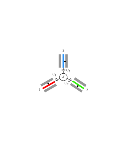
Figure 2: (color online) Setup for three cavities (1,2,3) coupled by a superconducting phase qubit $A$. Each cavity here is a one-dimensional coplanar waveguide transmission line resonator. The circle $A$ represents a superconducting phase qubit, which is capacitively coupled to cavity j via a capacitance $Cj$ ($j=1,2,3$). The three dark dots indicate the three superconducting phase qubits (1,2,3) embedded in the three cavities, respectively. The interaction of qubits (1,2,3) with their cavities are illustrated in Fig. 3(a,b,c), respectively. The interaction of the coupler qubit $A$ with the three cavities is shown in Fig. 3(d). Since three levels for each qubit is involved in our analysis, each qubit is renamed as a qutrit in Fig. 3

III POSSIBLE EXPERIMENTAL IMPLEMENTATION

The physical systems composed of cavities and superconducting qubits have been considered to be one of the most promising candidates for quantum information processing [30-34]. In above we have considered a general type of qubit. Let us now consider each qubit as a superconducting phase qubit and each cavity as a one-dimensional transmission line resonator. In addition, we assume that the coupler qubit $A$ is connected to each resonator via a coupler capacitance. As an example of the experimental implementation, we consider a setup in Fig. 2 for preparing the $W$ state of three superconducting phase qubits ($1,2,3$), which are embedded in the three one-dimensional transmission line resonators ($1,2,3$), respectively. To be more realistic, a third higher level $\left|2\right\rangle$ for each phase qubit here needs to be considered during the operations described above, since this level $\left|2\right\rangle$ may be excited due to the $\left|1\right\rangle\leftrightarrow\left|2\right\rangle$ transition induced by the cavity mode(s), which will turn out to affect the operation fidelity. Therefore, to quantify how well the proposed protocol works out, we will give an analysis of the operation fidelity, by taking this higher level $\left|2\right\rangle$ into account. Because of three levels being considered, we rename each qubit as a qutrit in the following.

When the intercavity crosstalk coupling and the unwanted $\left|1\right\rangle\leftrightarrow\left|2\right\rangle$ transition of each phase qutrit are considered, the Hamiltonian (1) is modified as follows

$$h_{I}=H_{I}+\Theta_{I},$$ (17)

where $H_{I}$ is the needed interaction Hamiltonian given in Eq. (1) above, while $\Theta_{I}$ is the unwanted interaction Hamiltonian, given by

$$\Theta_{I} = \sum_{j=1}^{3}\widetilde{g}_{j}\left(e^{i\widetilde{\delta}_{j}t}a_{j}\sigma_{21j}^{+}+h.c.\right)+\sum_{j=1}^{3}\widetilde{g}_{Aj}\left(e^{i\widetilde{\delta}_{Aj}t}a_{j}\sigma_{21A}^{+}+h.c.\right)$$ (18)

$$+\sum_{k\neq l;k,l=1}^{3}g_{kl}\left(e^{-i\Delta_{kl}t}a_{k}a_{l}^{+}+h.c.\right),$$

where $\sigma_{21j}^{+}=\left|2\right\rangle_{j}\left\langle 1\right|$ and $\sigma_{21A}^{+}=\left|2\right\rangle_{A}\left\langle 1\right|.$ The first term represents the unwanted off-resonant coupling between the mode of cavity $j$ and the $\left|1\right\rangle\leftrightarrow\left|2\right\rangle$ transition of qutrit $j$, with coupling constant $\widetilde{g}_{j}$ and detuning $\widetilde{\delta}_{j}=\omega_{21j}-\omega_{cj}$ [Fig. 3(a,b,c)], while the second term indicates the unwanted off-resonant coupling between the mode of cavity $j$ and the $\left|1\right\rangle\leftrightarrow\left|2\right\rangle$ transition of qutrit $A$, with coupling constant $\widetilde{g}_{Aj}$ and detuning $\widetilde{\delta}_{Aj}=\omega_{21A}-\omega_{cj}$ [Fig. 3(d)]. Here, the term describing the cavity-induced coherent $\left|0\right\rangle\leftrightarrow\left|2\right\rangle$ transition for each qutrit is not included in the Hamiltonian $\Theta_{I}$, since this transition is negligible because of $\omega_{cj}\ll\omega_{20j},\omega_{20A}$ ($j=1,2,3$) (Fig. 3). The last term of Eq. (18) describes the intercavity crosstalk between the three cavities, with $\Delta_{kl}=\omega_{ck}-\omega_{cl}=\delta_{l}-\delta_{k}$ (the frequency difference between two cavities $k$ and $l$) and $g_{kl}$ (the intercavity coupling constant between two cavities $k$ and $l$). Here and below, $kl\in\{12,13,23\}.$

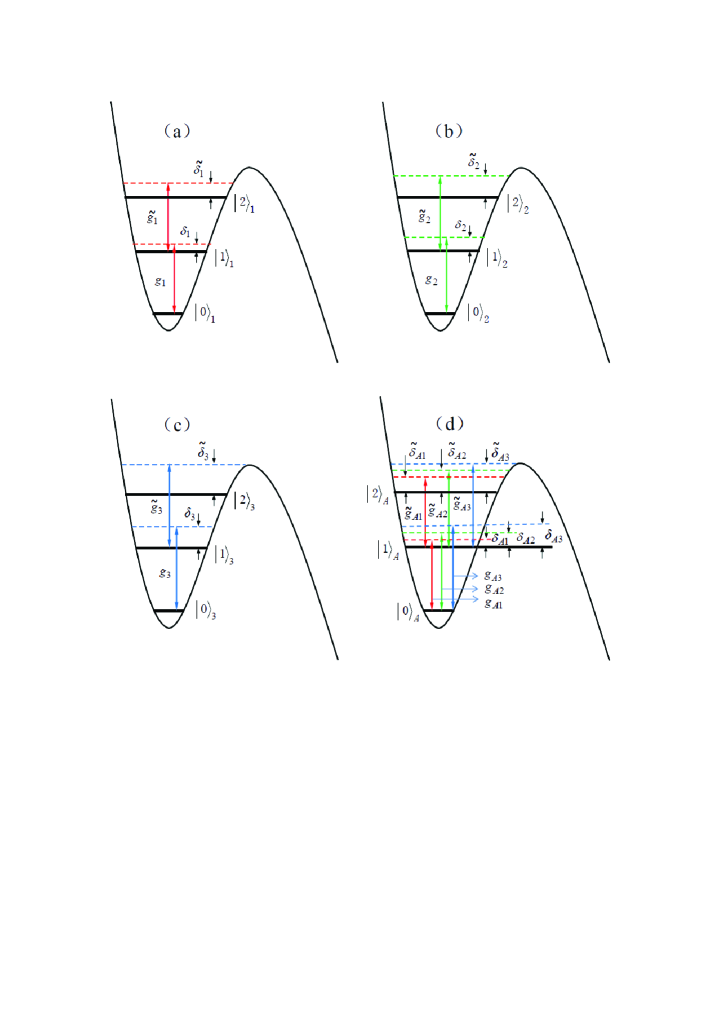
Figure 3: (Color online) Illustration of qutrit-cavity interaction. (a) Cavity $1$ is dispersively coupled to the $\left|0\right\rangle\leftrightarrow\left|1\right\rangle$ transition with coupling constant $g_{1}$ and detuning $\delta_{1},$ but far-off resonant (i.e., more detuned) with the $\left|1\right\rangle\leftrightarrow\left|2\right\rangle$ transition of qutrit $1$ with coupling consant $\widetilde{g}_{1}$ and detuning $\widetilde{\delta}_{1}$. (b) [and (c)] corresponds to the case that cavity $2$ ($3$) is dispersively coupled to the $\left|0\right\rangle\leftrightarrow\left|1\right\rangle$ transition but far-off resonant with the $\left|1\right\rangle\leftrightarrow\left|2\right\rangle$ transition of qutrit $2$ ($3$). (d) Cavities ($1,2,3$) dispersively interact with the $\left|0\right\rangle\leftrightarrow\left|1\right\rangle$ transition with coupling constants ($g_{A1},g_{A2},g_{A3}$) and detunings ($\delta_{A1},\delta_{A2},\delta_{A3}$), respectively; but they are far-off resonant with the $\left|1\right\rangle\leftrightarrow\left|2\right\rangle$ transition of qutrit $A$ with coupling constants ($\widetilde{g}_{A1},\widetilde{g}_{A2},\widetilde{g}_{A3}$) and detunings $\widetilde{\delta}_{A1},\widetilde{\delta}_{A2},\widetilde{\delta}_{A3}$), respectively. Here, $\delta_{j}=\omega_{10j}-\omega_{cj},\widetilde{\delta}_{j}=\omega_{21j}-\omega_{cj},\delta_{Aj}=\omega_{10A}-\omega_{cj},$ and $\widetilde{\delta}_{Aj}=\omega_{21A}-\omega_{cj}$ ($j=1,2,3$), where $\omega_{10j}$ ($\omega_{21j}$) is the $\left|0\right\rangle\leftrightarrow\left|1\right\rangle$ ($\left|1\right\rangle\leftrightarrow\left|2\right\rangle$) transition frequency of qutrit $j$, $\omega_{10A}$ ($\omega_{21A}$) is the $\left|0\right\rangle\leftrightarrow\left|1\right\rangle$ ($\left|1\right\rangle\leftrightarrow\left|2\right\rangle$) transition frequency of qutrit $A$, and $\omega_{cj}$ is the frequency of cavity $j$.

The dynamics of the lossy system, with finite qutrit relaxation and dephasing and photon lifetime included, is determined by the following master equation

$$\frac{d\rho}{dt} = -i\left[h_{I},\rho\right]+\sum_{j=1}^{3}\kappa_{j}\mathcal{L}\left[a_{j}\right]$$ (19)

$$+\sum_{j=1,2,3,A}\left\{\gamma_{j}\mathcal{L}\left[\sigma_{j}^{-}\right]+\gamma_{21j}\mathcal{L}\left[\sigma_{21j}^{-}\right]+\gamma_{20j}\mathcal{L}\left[\sigma_{20j}^{-}\right]\right\}$$

$$+\sum_{j=1,2,3,A}\left\{\gamma_{j,\varphi 1}\left(\sigma_{11j}\rho\sigma_{11j}-\sigma_{11j}\rho/2-\rho\sigma_{11j}/2\right)\right\}$$

$$+\sum_{j=1,2,3,A}\left\{\gamma_{j,\varphi 2}\left(\sigma_{22j}\rho\sigma_{22j}-\sigma_{22j}\rho/2-\rho\sigma_{22j}/2\right)\right\},\ \ \ \$$

where $\sigma_{20j}^{-}=\left|0\right\rangle_{j}\left\langle 2\right|,\sigma_{20A}^{-}=\left|0\right\rangle_{A}\left\langle 2\right|,\sigma_{11j}=\left|1\right\rangle_{j}\left\langle 1\right|,\sigma_{22j}=\left|2\right\rangle_{j}\left\langle 2\right|;$ and $\mathcal{L}\left[\Lambda\right]=\Lambda\rho\Lambda^{+}-\Lambda^{+}\Lambda\rho/2-\rho\Lambda^{+}\Lambda/2,$ with $\Lambda=a_{j},\sigma_{j}^{-},\sigma_{21j}^{-},\sigma_{20j}^{-}.$ Here, $\kappa_{j}$ is the photon decay rate of cavity $a_{j}$ ($j=1,2,3$). In addition, $\gamma_{j}$ is the energy relaxation rate of the level $\left|1\right\rangle$ of qutrit $j$, $\gamma_{21j}$ ($\gamma_{20j}$) is the energy relaxation rate of the level $\left|2\right\rangle$ of qutrit $j$ for the decay path $\left|2\right\rangle\rightarrow\left|1\right\rangle$ ($\left|0\right\rangle$), and $\gamma_{j,\varphi 1}$ ($\gamma_{j,\varphi 2}$) is the dephasing rate of the level $\left|1\right\rangle$ ($\left|2\right\rangle$) of qutrit $j$ ($j=1,2,3,A$).

The fidelity of the operation is given by

$$\mathcal{F}=\left\langle\psi_{\mathrm{id}}\right|\widetilde{\rho}\left|\psi_{\mathrm{id}}\right\rangle,$$ (20)

where $\left|\psi_{\mathrm{id}}\right\rangle$ is the output state $\left|W_{2,1}\right\rangle\left|0\right\rangle_{A}\left|0\right\rangle_{c1}\left|0\right\rangle_{c2}\left|0\right\rangle_{c3}$ of an ideal system (i.e., without dissipation, dephasing, and crosstalk) as discussed in the previous section; and $\widetilde{\rho}$ is the final density operator of the system when the operation is performed in a realistic physical system.

Without loss of generality, let us consider three identical superconducting phase qutrits. According to the condition (4), we set $\delta_{1}/\left(2\pi\right)=\delta_{A1}/\left(2\pi\right)=-0.5$ GHz, $\delta_{2}/\left(2\pi\right)=\delta_{A2}/\left(2\pi\right)=-1$ GHz, and $\delta_{3}/\left(2\pi\right)=\delta_{A3}/\left(2\pi\right)=-1.5$ GHz. For the setting here, we have $\Delta_{12}/2\pi=-0.5$ GHz, $\Delta_{13}/2\pi=-1.0$ GHz, and $\Delta_{23}/2\pi=-0.5$ GHz. Set $\widetilde{\delta}_{j}=\delta_{j}-0.05\omega_{10j}$ and $\widetilde{\delta}_{Aj}=\delta_{Aj}-0.05\omega_{10A}$ ($j=1,2,3$) [35]. For superconducting phase qubits, the typical qubit transition frequency is between 4 and 10 GHz. Thus, we choose $\omega_{10A}/2\pi,\omega_{10j}/2\pi\sim 6.5$ GHz. Note that $g_{2}$ ($g_{3}$) is determined based on Eq. (8), given $\delta_{1},$ $\delta_{2}$ ($\delta_{3}$), and $g_{1}.$ In addition, $g_{Aj}$ is determined by Eq. (15), given $g_{j}$ ($j=1,2,3$). For the present case, we have $n=3.$ Next, one has $\widetilde{g}_{j}\sim\sqrt{2}g_{j}$ and $\widetilde{g}_{Aj}\sim\sqrt{2}g_{Aj}$ ($j=1,2,3$) for the phase qutrit here. We choose $\gamma_{j,\varphi 1}^{-1}=\gamma_{j,\varphi 2}^{-1}=2.5$ $\mu$s, $\gamma_{j}^{-1}=10$ $\mu$s, $\gamma_{21j}^{-1}=7.5$ $\mu$s, and $\gamma_{20j}^{-1}=30$ $\mu$s; and $\kappa_{j}^{-1}=5$ $\mu$s ($j=1,2,3$). For a phase qutrit with the three levels considered here, the $\left|0\right\rangle\leftrightarrow\left|2\right\rangle$ dipole matrix element is much smaller than that of the $\left|0\right\rangle\leftrightarrow\left|1\right\rangle$ and $\left|1\right\rangle\leftrightarrow\left|2\right\rangle$ transitions. Thus, $\gamma_{20j}^{-1}\gg\gamma_{10j}^{-1},\gamma_{21j}^{-1}.$

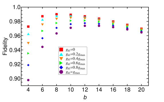
Figure 4: (Color online) Fidelity of the $W$-state preparation versus the normalized detuning $b=\left|\delta_{1}\right|/g_{1}$. Refer to the text for the parameters used in the numerical calculation. Here, $g_{kl}$ are the coupling strengths between cavities $k$ and $l$ ( $k\neq l;\,k,l\in\left\{1,2,3\right\}$), which are taken to be the same for simplicity.

For the parameters chosen above, the fidelity versus $b=\left|\delta_{1}\right|/g_{1}$ is plotted in Fig. 4 for $g_{kl}=0,0.2g_{\max},$ $0.4g_{\max},0.6g_{\max},0.8g_{\max},g_{\max},$ where $g_{\max}=\max\{g_{A1},g_{A2},g_{A3}\}.$ Fig. 4 shows that for $g_{kl}\leq 0.2g_{\max}$, the effect of intercavity cross coupling between the three cavities on the operational fidelity is negligible, which can be seen by comparing the top two curves. In addition, it can be seen from Fig. 4 that for $b\sim 8$ and $g_{kl}=0.2g_{\max},$ a high fidelity $\sim 99\%$ is available for the $W$-state preparation.

The condition $g_{kl}\leq 0.2g_{\max}$ is not difficult to satisfy with the typical capacitive cavity-qutrit coupling illustrated in Fig. 2. As long as the cavities are physically well separated, the intercavity cross-talk coupling strength is $g_{kl}\sim g_{Ak}C_{l}/C_{\Sigma},g_{Al}C_{k}/C_{\Sigma},$ where $C_{\Sigma}=C_{1}+C_{2}+C_{3}+C_{q}$. With a choice of $C_{1},C_{2},C_{3}\sim 1$ fF and $C_{\Sigma}\sim 10^{2}$ fF (the typical values of the cavity-qutrit coupling capacitance and the sum of all coupling capacitance and qutrit self-capacitance, respectively), one has $g_{kl}\sim 0.01g_{Ak},0.01g_{Al}$. Because of $g_{A1,}$ $g_{A2,}$ $g_{A3}\leq g_{\max},$ the condition $g_{kl}\leq 0.2g_{\max}$ can be readily met in experiments. Thus, it is straightforward to implement designs with sufficiently weak direct intercavity couplings.

For $b\sim 8$, we have $\{g_{1},g_{2},g_{3},g_{A1},g_{A2},g_{A3}\}\sim$ $\{62.5,88.4,108.3,36.1,51.0,62.5\}$ MHz. Experimentally, a coupling constant $\sim 220$ MHz can be reached for a superconducting qutrit coupled to a one-dimensional CPW (coplanar waveguide) resonator [36,37], and that $T_{1}$ and $T_{2}$ can be made to be on the order of $10-100$ $\mu$s or longer for state-of-the-art superconducting devices [38-42]. For phase qutrits, the energy relaxation time $T_{1}^{{}^{\prime}}$ and dephasing time $T_{2}^{\prime}$ of the level $\left|2\right\rangle$ are, respectively, comparable to $T_{1}$ and $T_{2}$ because of $T_{1}^{\prime}\sim T_{1}/\sqrt{2}$ and $T_{2}^{{}^{\prime}}\sim T_{2}.$ With $\omega_{10A}/2\pi,\omega_{10j}/2\pi\sim 6.5$ GHz chosen above, we have $\omega_{c1}/2\pi\sim 6.0$ GHz, $\omega_{c2}/2\pi\sim$ $5.5$ GHz, and $\omega_{c3}/2\pi\sim$ $5.0$ GHZ. For these cavity frequencies and the values of $\kappa_{1}^{-1},\kappa_{2}^{-1}$ and $\kappa_{3}^{-1}$ used in the numerical calculation, the required quality factors for the three cavities are $Q_{1}\sim 1.9\times 10^{5},$ $Q_{2}\sim 1.7\times 10^{5},$ and $Q_{3}\sim 1.6\times 10^{5},$ respectively. It should be mentioned that superconducting CPW resonators with a loaded quality factor $Q\sim 10^{6}$ have been experimentally demonstrated [43,44], and planar superconducting resonators with internal quality factors above one million ($Q>10^{6}$) have also been recently reported [45]. Our analysis given here demonstrates that high-fidelity preparation of the $W$ state of three intracavity qubits by using this proposal is feasible within the present circuit QED technique. We remark that further investigation is needed for each particular experimental setup. However, it requires a rather lengthy and complex analysis, which is beyond the scope of this theoretical work.

IV CONCLUSION

We have proposed a general method to generate the $W$-class entangled states of $n$ qubits distributed in different $n$ cavities. As shown above, this proposal offers some advantages and features: the entanglement preparation does not employ cavity photons as quantum buses, thus decoherence caused due to the cavity decay is greatly suppressed during the operation; only one coupler qubit is needed to connect with all cavities such that the circuit complex is greatly reduced; moreover, only one step of operation is required and no classical pulse is needed, so that the operation is much simplified. The time required decreases as the number of qubits increases. In addition, our numerical simulation shows that high-fidelity implementation of the three-qubit $W$ state is feasible for the current circuit QED technology. The method presented here is also applicable to a wide range of physical implementations with different types of qubits such as quantum dots, superconducting qubits (e.g., phase, flux and charge qubits), NV centers, and atoms.

References

- (1) W. Dür, G. Vidal, Three qubits can be entangled in two inequivalent ways, and J. I. Cirac, Phys. Rev. A 62, 062314 (2000).
- (2) D. M. Greenberger et al., Bell s theorem without inequalities, Am. J. Phys. 58, 1131 (1990).
- (3) V.N. Gorbachev et al., Can the states of the W-class be suitable for teleportation?, Phys. Lett. A 314, 267 (2003).
- (4) J. Joo et al., Quantum teleportation via a W state, New J. Phys. 5, 136 (2003).
- (5) J. Joo et al., Quantum Secure Communication with W States, arXiv:quant-ph/0204003 (2002).
- (6) S. S. Sharma and E. Almeida, J. Phys. B 41, 165503 (2008).
- (7) G. X. Li, Generation of pure multipartite entangled vibrational states for ions trapped in a cavity, Phys. Rev. A 74, 055801 (2006).
- (8) P. Xue and G. C. Guo, Scheme for preparation of mulipartite entanglement of atomic ensembles, Phys. Rev. A 67, 034302, 2003.
- (9) Y. Gao, H. Zhou, D. Zou, X. Peng, and J. Du, Preparation of Greenberger-Horne-Zeilinger and W states on a one-dimensional Ising chain by global control, Phys. Rev. A 87, 032335 (2013).
- (10) A. Perez-Leija, J. C. Hernandez-Herrejon, H. Moya-Cessa, Generating photon-encoded W states in multiport waveguide-array systems, Phys. Rev. A 87, 013842 (2013).
- (11) C. S. Yu, X. X. Yi, H. S. Song, and D. Mei, Robust preparation of Greenberger-Horne-Zeilinger and W states of three distant atoms, Phys. Rev. A 75, 044301 (2007).
- (12) X. B. Zou, K. Pahlke, and W. Mathis, Generation of an entangled four-photon W state, Phys. Rev. A 66, 044302 (2002).
- (13) T. Yamamoto, K. Tamaki, M. Koashi, and N. Imoto, Polarization-entangled W state using parametric down-conversion, Phys. Rev. A 66, 064301 (2002).
- (14) X. Wang, M. Feng, and B. C Sanders, Multipartite entangled states in coupled quantum dots and cavity QED, Phys. Rev. A 67, 022302 (2003).
- (15) K. H. Song, Z. W. Zhou, and G. C. Guo, Quantum logic gate operation and entanglement with superconducting quantum interference devices in a cavity via a Raman transition, Phys. Rev. A 71, 052310 (2005); K. H. Song, S. H. Xiang, Q. Liu, and D. H. Lu, Quantum computation and W-state generation using superconducting flux qubits coupled to a cavity without geometric and dynamical manipulation, Phys. Rev. A 75, 032347 (2007).
- (16) X.L. Zhang, K.L. Gao, and M. Feng, Preparation of cluster states and W states with superconducting quantum-interference-device qubits in cavity QED, Phys. Rev. A 74, 024303 (2006); Z. J. Deng, K. L. Gao, and M. Feng, Generation of N-qubit W states with rf SQUID qubits by adiabatic passage, Phys. Rev. A 74, 064303 (2006).
- (17) A. Biswas and G. S. Agarwal, J. Mod. Opt. 51, 1627 (2004).
- (18) R. Sweke, I. Sinayskiy, and F. Petruccione, Dissipative preparation of large W states in optical cavities, Phys. Rev. A 87, 042323 (2013).
- (19) H. Häffner, W. Hänsel, C. F. Roos, J. Benhelm, D. Chek-al-kar, M. Chwalla, T. Koärber, U. D. Rapol, M. Riebe, P. O. Schmidt, C. Becher, O. Gühne, W. Dür, and R. Blatt, Scalable multiparticle entanglement of trapped ions, Nature 438, 643 (2005).
- (20) S. B. Papp, K. S. Choi, H. Deng, P. Lougovski, S. J. van Enk, and H. J. Kimble, Characterization of Multipartite Entanglement for One Photon Shared Among Four Optical Modes, Science 324, 764 (2009).
- (21) M. Neeley, R. C. Bialczak, M. Lenander, E. Lucero, M. Mariantoni, A. D. O’Connell, D. Sank, H. Wang, M. Weides, J. Wenner, Y. Yin, T. Yamamoto, A. N. Cleland, and J. M. Martinis, Generation of three-qubit entangled states using superconducting phase qubits, Nature 467, 570 (2010).
- (22) K. S. Choi, A. Goban, S. B. Papp, S. J. van Enk, and H. J. Kimble, Entanglement of spin waves among four quantum memories, Nature 468, 412 (2010).
- (23) F. Altomare, J. I. Park, K. Cicak, M. A. Sillanpää, M. S. Allman, D. Li, A. Sirois, J. A. Strong, J. D. Whittaker, and R.W. Simmonds, Tripartite interactions between two phase qubits and a resonant cavity, Nature Physics 6, 777 (2010).
- (24) S. B. Zheng and G. C. Guo, Efficient Scheme for Two-Atom Entanglement and Quantum Information Processing in Cavity QED, Phys. Rev. Lett. 85, 2392 (2000).
- (25) S. B. Zheng, One-Step Synthesis of Multiatom Greenberger-Horne-Zeilinger States, Phys. Rev. Lett. 87, 230404 (2011).
- (26) J. Clarke and F. K. Wilhelm, Superconducting quantum bits, Nature 453, 1031 (2008).
- (27) M. Neeley, M. Ansmann, R. C. Bialczak, M. Hofheinz, N. Katz, E. Lucero, A. OConnell, H. Wang, A. N. Cleland, and J. M. Martinis, Process tomography of quantum memory in a Josephson-phase qubit coupled to a two-level state, Nature Phys. 4, 523 (2008).
- (28) S. Han, J. Lapointe, and J. E. Lukens: in Single-Electron Tunneling and Mesoscopic Devices, Springer Series in Electronics and Photonics, Vol. 31 (Springer, Berlin, 1991), pp. 219 . 222.
- (29) M. Sandberg, C. M. Wilson, F. Persson, T. Bauch, G. Johansson, V. Shumeiko, T. Duty, and P. Delsing, Tuning the field in a microwave resonator faster than the photon lifetime, Appl. Phys. Lett. 92, 203501 (2008).
- (30) A. Blais, R.-S. Huang, A. Wallraff, S. M. Girvin, and R. J. Schoelkopf, Cavity quantum electrodynamics for superconducting electrical circuits: An architecture for quantum computation, Phys. Rev. A 69, 062320 (2004).
- (31) J. Q. You and F. Nori, Superconducting circuits and quantum information, Phys. Today 58 [11], 42 (2005).
- (32) J. Q. You and F. Nori, Atomic physics and quantum optics using superconducting circuits, Nature 474, 589 (2011).
- (33) Z. L. Xiang, S. Ashhab, J. Q. You, and F. Nori, Hybrid quantum circuits: Superconducting circuits interacting with other quantum systems, Rev. Mod. Phys. 85, 623 (2013).
- (34) C. P. Yang, Shih-I. Chu, and S. Han, Quantum Information Transfer and Entanglement with SQUID Qubits in Cavity QED: A Dark-State Scheme with Tolerance for Nonuniform Device Parameter, Phys. Rev. A 67, 042311 (2003); Phys. Rev. Lett. 92, 117902 (2004).
- (35) For a phase qutrit, a ratio of the anharmonicity between the transition frequency and the transition frequency to the the transition frequency is readily achieved in experiments.
- (36) M. A. Sillanpää, J. Li, K. Cicak, F. Altomare, J. I. Park, R. W. Simmonds, G. S. Paraoanu, and P. J. Hakonen, Autler-Townes Effect in a Superconducting Three-Level System, Phys. Rev. Lett. 103, 193601 (2009).
- (37) L. DiCarlo et al., Preparation and measurement of three-qubit entanglement in a superconducting circuit, Nature 467, 574 (2010).
- (38) J. Bylander et al., Noise spectroscopy through dynamical decoupling with a superconducting flux qubit, Nature Phys. 7, 565 (2011).
- (39) H. Paik, Observation of High Coherence in Josephson Junction Qubits Measured in a Three-Dimensional Circuit QED Architecture, Phys. Rev. Lett. 107, 240501 (2011).
- (40) J. M. Chow et al., Universal Quantum Gate Set Approaching Fault-Tolerant Thresholds with Superconducting Qubits, Phys. Rev. Lett. 109, 060501 (2012).
- (41) C. Rigetti et al., Superconducting qubit in a waveguide cavity with a coherence time approaching 0.1 ms, Phys. Rev. B 86, 100506(R) (2012).
- (42) R. Barends et al., Coherent Josephson Qubit Suitable for Scalable Quantum Integrated Circuits, Phys. Rev. Lett. 111, 080502 (2013).
- (43) W. Chen, D. A. Bennett, V. Patel, and J. E. Lukens, Substrate and process dependent losses in superconducting thin film resonators, Supercond. Sci. Technol. 21, 075013 (2008).
- (44) P. J. Leek, M. Baur, J. M. Fink, R. Bianchetti, L. Steffen, S. Filipp, and A. Wallraff, Cavity Quantum Electrodynamics with Separate Photon Storage and Qubit Readout Modes, Phys. Rev. Lett. 104, 100504 (2010).
- (45) A. Megrant et al., Planar superconducting resonators with internal quality factors above one million, Appl. Phys. Lett. 100, 113510 (2012).