On the shallow atmosphere approximation in finite element dynamical cores

Abstract

We provide an approach to implementing the shallow atmosphere approximation in three dimensional finite element discretisations for dynamical cores. The approach makes use of the fact that the shallow atmosphere approximation metric can be obtained by writing equations on a three-dimensional manifold embedded in $\mathbb{R}^{4}$ with a restriction of the Euclidean metric. We show that finite element discretisations constructed this way are equivalent to the use of a modified three dimensional mesh for the construction of metric terms. We demonstrate our approach via a convergence test for a prototypical elliptic problem.

1 Introduction

The shallow atmosphere approximation is a commonly used simplifying approximation in the development of atmosphere and ocean dynamical cores (Phillips, 1966; White et al., 2005) where factors of $1/r$ are replaced by $1/a$, where $r$ is the radial coordinate and $a$ is some reference value (typically the Earth’s mean radius). Additionally, some of the metric terms in the momentum equation are neglected. The approximation amounts to neglecting the increase with $r$ of the surface area of a spherical shell with radius $r$. Müller (1989) (see also White et al. (2005)) showed that the shallow atmosphere approximation is equivalent to solving the equations of motion in a geometry with a non-Euclidean metric. Thuburn and White (2013) showed that this metric can be obtained by considering the restriction of the four-dimensional Euclidean metric to the three-manifold embedded in four-dimensional space that consists of the surface of a sphere extruded into the fourth direction (they also discussed the interesting aspect of non-unique geodesics in this geometry which cause difficulties for computing Lagrangian trajectories). We shall make use of this viewpoint in this paper. The shallow atmosphere approximation is usually combined with the traditional approximation, which neglects the horizontal component of the rotation vector in the Coriolis term. This combination has historically been used to obtain an equation set with a conserved energy and potential vorticity; we note that an energy and PV conserving formulation of the shallow atmosphere approximation with non-traditional Coriolis term has recently been discovered (Tort and Dubos, 2014).

In recent years there has been much interest in using finite element methods for developing atmospheric dynamical cores (Ullrich, 2014; Nair et al., 2009; Dennis et al., 2011), mostly because they can avoid the parallel scalability problems associated with a latitude-longitude grid. In particular, the NERC/UK Met Office/STFC dynamical core project, nicknamed “Gung Ho”, is considering compatible/mimetic mixed finite element methods (Cotter and Shipton, 2012), which serve as an extension of the C-grid staggered finite difference method, as the basis for dynamical core development. One option is to use a finite element method for the horizontal discretisation and a conventional finite difference discretisation for the vertical discretisation, with either Lorenz or Charney-Phillips staggering. However, it is also attractive to consider fully three-dimensional finite element discretisations (using, for example, prismatic elements arranged in columns) since they allow more flexibility with terrain-following meshes.

Whilst several dynamical cores (the UK Met Office Unified Model, for example) do not use the shallow atmosphere approximation in operational mode, it is useful to include a minimally pervasive shallow atmosphere approximation option since many of the standard test cases use it. In addition, many other dynamical cores are shallow atmosphere only, and so such an option is necessary for dynamical core intercomparison studies. Implementation of the shallow atmosphere approximation in a three-dimensional finite element model is not immediately straightforward: in contrast to finite difference methods where the metric terms appear explicitly in the discretisation, finite element methods can use Cartesian coordinates, with derivatives being automatically computed via a transformation of each element in the mesh to a standard reference element where all differentiation and integration is performed with the result that the metric terms do not appear explicitly in the discretisation. This leads to the question of how to apply the shallow atmosphere approximation within a three-dimensional finite element approximation. The solution lies in the use of the transformation from four-dimensional space discussed in Thuburn and White (2013), referred to above. By first mapping the equations onto the embedded 3-manifold in four dimensional space, and then transforming back to the reference element, we obtain equations which are equivalent to the shallow atmosphere approximation.

The rest of this paper is organised as follows. In Section 2 we review the calculus tools associated with the shallow atmosphere approximation. In Section 3, we explain our approach to implementing the shallow atmosphere approximation in finite element models. We then illustrate this approach with a numerical convergence test in Section 4, and finally provide a summary and outlook in Section 5.

2 Shallow atmosphere approximation through pullback

In this section, we review the necessary calculus tools to form shallow atmosphere approximations of equations. We are interested in solving equations in the spherical annulus domain

$$\begin{split}M&=\left\{\boldsymbol{x}=(x_{1},x_{2},x_{3})\in\mathbb{R}^{3}:\right.\\ &\qquad\qquad\left.a^{2}\leq x^{2}_{1}+x^{2}_{2}+x^{2}_{3}\leq(a+H)^{2}\right\}\subset\mathbb{R}^{3},\end{split}$$ (1)

where $a$ denotes the radius of the interior spherical surface and $H$ denotes the thickness of the spherical annulus. As discussed in Thuburn and White (2013), the shallow atmosphere approximation can be obtained by writing equations in the domain

$$\begin{split}\tilde{M}&=\left\{\tilde{\boldsymbol{x}}=(\tilde{x}_{1},\tilde{x}_{2},\tilde{x}_{3},\tilde{x}_{4})\in\mathbb{R}^{4}:\right.\\ &\left.\qquad\qquad a^{2}=\tilde{x}^{2}_{1}+\tilde{x}^{2}_{2}+\tilde{x}^{2}_{3},\,0\leq\tilde{x}_{4}\leq H\right\}\subset\mathbb{R}^{4},\\ \end{split}$$ (2)

and transforming to the physical domain $M$ using the smooth invertible map $\Phi:\tilde{M}\to M$ defined by

$$\tilde{\boldsymbol{x}}=(\tilde{x}_{1},\tilde{x}_{2},\tilde{x}_{3},\tilde{x}_{4})\mapsto\boldsymbol{x}=\Phi(\tilde{\boldsymbol{x}})=\left(1+\frac{\tilde{x}_{4}}{a}\right)(\tilde{x}_{1},\tilde{x}_{2},\tilde{x}_{3}).$$ (3)

This transformation contains two aspects. Firstly, all derivatives must be modified using the chain rule. Secondly, the various physical quantities must be transformed as follows:

1. Scalar quantities (such as potential temperature) must be transformed according to

   $$\tilde{\theta}\mapsto\theta=\tilde{\theta}\circ\Phi^{-1}.$$ (4)

2. Vector fields (such as the velocity field) must be transformed according to

   $$\tilde{\boldsymbol{u}}\mapsto\boldsymbol{u}=\left(J\circ\Phi^{-1}\right)^{-T}\tilde{\boldsymbol{u}}\circ\Phi^{-1},\quad J:=\tilde{\nabla}\Phi,$$ (5)

   where the superscript ^-T indicates the transpose of the inverse. Since we have a mapping from a 3-manifold $\tilde{M}$ embedded in $\mathbb{R}^{4}$ to $\mathbb{R}^{3}$, the inverse is defined on the tangent space to $\tilde{M}$. If the $\mathbb{R}^{4}$ coordinate system is used to represent tangent vectors, then the Moore-Penrose inverse of $J$ should be used.

3. Fluxes (i.e., vector quantities that must be integrated over surfaces to obtain flow rates, such as the mass flux) must be transformed according to

   $$\tilde{\boldsymbol{F}}\mapsto\boldsymbol{F}=\frac{1}{\det J}\left(J\circ\Phi^{-1}\right)\tilde{\boldsymbol{F}}\circ\Phi^{-1},$$ (6)

   where $\det J$ is the pseudodeterminant of $J$, namely the product of the non-zero singular values of $J$.

4. Densities (i.e., scalar quantities that must be integrated over volumes to obtain total quantities, such as kinetic energy density) must be transformed according to

   $$\tilde{\rho}\mapsto\rho=\frac{1}{\det J}\tilde{\rho}\circ\Phi^{-1}.$$ (7)

The resulting evolution equations for the quantities in $M$ will then contain metric terms that encode the shallow atmosphere approximation.

For example, we could take the velocity equation and write it on $\tilde{M}$ as

$$\frac{\partial\tilde{\boldsymbol{u}}}{\partial t}+(\tilde{\boldsymbol{u}}\cdot\nabla)\tilde{\boldsymbol{u}}+2\tilde{\boldsymbol{\Omega}}{\times}\tilde{\boldsymbol{u}} =-\tilde{\theta}\nabla p+\nabla\tilde{\phi}+\boldsymbol{l}\lambda,$$ (8)

$$\boldsymbol{l}\cdot\tilde{\boldsymbol{u}} =0,$$ (9)

where $\tilde{\boldsymbol{u}}$ is the velocity field, $\tilde{\theta}$ is the potential temperature, $\tilde{p}$ is the pressure, and $\tilde{\phi}$ is the geopotential, all defined on $\tilde{M}$. Further, $\boldsymbol{l}$ is the unit vector that is normal to all tangent vectors on $\tilde{M}$, $\lambda$ is a Lagrange multiplier field that enforces the condition that $\tilde{\boldsymbol{u}}$ stays tangential to $\tilde{M}$, and the gradient operator $\nabla$ is restricted to the tangent space on $\tilde{M}$.

The cross-product of two vector fields $\tilde{\boldsymbol{u}}$ and $\tilde{\boldsymbol{v}}$ on the 3-manifold $\tilde{M}$ is defined in the usual way as

$$\tilde{\boldsymbol{u}}\times\tilde{\boldsymbol{v}}=\|\tilde{\boldsymbol{u}}\|\|\tilde{\boldsymbol{v}}\|\sin\theta\boldsymbol{n},$$ (10)

where $\theta$ is the angle between $\tilde{\boldsymbol{u}}$ and $\tilde{\boldsymbol{v}}$, and $\boldsymbol{n}$ is the unit vector perpendicular to both $\tilde{\boldsymbol{u}}$ and $\tilde{\boldsymbol{v}}$ but still in the tangent space to $\tilde{M}$, with the sign determined according to the right-hand rule as usual. This can be computed by finding an orthonormal basis for the tangent space at each point, expanding $\tilde{u}$ and $\tilde{v}$ in that basis and using the standard formula for the corresponding components of $\tilde{w}$. We could also make the traditional approximation, so that

$$\tilde{\boldsymbol{\Omega}}=\frac{\Omega x_{3}}{r^{2}}\left(x_{1},x_{2},x_{3},0\right),\quad r^{2}=x_{1}^{2}+x_{2}^{2}+x_{3}^{2},$$ (11)

where $\Omega$ is a scalar constant. In which case we obtain

$$\tilde{\boldsymbol{\Omega}}\times\tilde{\boldsymbol{u}}=\frac{\Omega x_{3}}{r^{2}}\left(x_{2}u_{3}-x_{3}u_{2},-x_{1}u_{3}+x_{3}u_{1},x_{1}u_{2}-x_{2}u_{1},u_{4}\right).$$ (12)

To extend these ideas to domains with varying topography, we keep the same transformation map $\Phi$ from Equation (3), but modify the corresponding domains $M$ and $\tilde{M}$.

3 Finite element methods for the shallow atmosphere approximation

Dynamical cores using finite difference discretisations are usually developed by starting with the equations written in spherical polar coordinates. This can be thought of as writing the equations (such as (8)) on $M$, applying the chain rule to the coordinate change from $M$ into spherical coordinates, and applying the appropriate transformations to all of the physical quantities. This transformation leads to metric terms appearing in the equations. Conversely, the shallow atmosphere approximation is obtained by writing the equations on $\tilde{M}$ and transforming from there instead of $M$, leading to relevant alterations of the metric terms.

In contrast, when using a finite element discretisation it is often more natural to keep everything in Cartesian coordinates on $M$, particularly since this then avoids the awkward problem of how to discretise the spherical coordinate metric terms whilst maintaining conservation, stability, etc. Hence, we propose to obtain finite element discretisations of the shallow atmosphere approximation by solving Equation (8) in $\tilde{M}$ (together with the equations of motion for the other quantities) before finally transforming back to spherical coordinates to produce the results. If integral quantities are required for postprocessing, such as circulation loop integrals of velocities, flux integrals through surfaces, or volume integrals, then the metric terms must be included otherwise the correct conservation properties will not be observed. The easiest way to do this is to compute these quantities directly on $\tilde{M}$.

To begin, we define an approximation to the curved manifold $\tilde{M}$ by selecting a discrete set of points in $\tilde{M}$ and then using these points as vertices in a mesh. We denote this mesh by $\tilde{M}^{\delta}$. This choice also defines a mesh approximating $M$ in $\mathbb{R}^{3}$ which we denote $M^{\delta}:=\Phi(\tilde{M}^{\delta})$.

In contrast to finite different methods, rather than discretising the operators in the PDE, we choose discrete function spaces defined on $\tilde{M}^{\delta}$ in which we seek a solution weakly (i.e. in integral form). The core of the finite element method therefore boils down to integrating known functions over the domain $\tilde{M}^{\delta}$, typically via numerical quadrature. These integrals may be rewritten as sums of integrals over the individual elements making up $\tilde{M}^{\delta}$. The integration is then performed by transforming from each individual physical element to a reference element $\hat{e}$. This merely requires that we have a transformation $g_{e}$ from the reference element to each physical element $e$: gradients are then computed by the change-of-variables formula requiring the inverse of the Jacobian $J_{e}$ of $g_{e}$.

This extends naturally to problems solved on an n-dimensional manifold $\mathcal{M}$ embedded in $\mathbb{R}^{m},\>m>n$, as described in Rognes et al. (2013). We just need to be careful since $J_{e}$ is no longer square and its inverse is therefore not well-defined. It may, however, be inverted under the assumption that the solution lies in the tangent space of $\mathcal{M}$ by using the Moore-Penrose inverse.

For large-scale geophysical flows it is usually desirable to use finite element meshes arranged in vertical columns, resulting in prismatic elements as shown in figure 1. In contrast to tetrahedral elements, if prismatic elements are used, meshes of the spherical annulus domain $M$ will result in the transformation $g_{e}$ from the reference element to the physical element being non-affine (affine meaning the combination of a translation and a linear map). This is because the triangle at the top of each prismatic element in the mesh is larger than than the triangle at the bottom. The result is that $J_{e}$ is not constant within each element and must be recalculated (and if necessary, inverted) at each quadrature point. In the absence of varying topography, and in the case of elements with straight sides in $\mathbb{R}^{4}$, a useful side-effect of the shallow atmosphere approximation is that this area increase does not occur in $\tilde{M}$. Hence $g_{e}$ is affine and $J_{e}$ need only be computed (and inverted) once per element, reducing the required number of floating point operations.

Figure 1: Mapping from 3-dimensional reference prismatic element to a physical element in the spherical annulus. Note how the physical element has an increasing area when moving radially outwards, such that $g_{e}$ is non-affine.

3.1 Solving in 4-d

Many finite element software libraries do not contain the capability to solve equations on embedded manifolds in higher-dimensional spaces. Further, the Fenics 1.2 implementation of Rognes et al. (2013) did not consider the case of a 3-manifold embedded in $\mathbb{R}^{4}$. One alternative would be to solve the equations in $\mathbb{R}^{3}$ but include the metric terms obtained from the transformation from $\tilde{M}$. However, this would be a very pervasive change, since it changes the equations at the element integral level, and therefore limits the possibilities for using shallow atmosphere approximation tests to build up confidence in the deep atmosphere version of a dynamical core. Fortunately, we can circumvent this problem by composing two transformations: the first ($\tilde{g}_{e}$) from the reference element $\hat{e}\subset\mathbb{R}^{3}$ into $\tilde{M}^{\delta}\subset\mathbb{R}^{4}$; the second ($g_{e}$) from $\hat{e}$ into $\mathbb{R}^{3}$. The relationship between these transformations is sketched in figure 2.

Figure 2: Transformations between the reference element ($\hat{e}$) and physical elements in $\mathbb{R}^{4}$ ($\tilde{e}$) and $\mathbb{R}^{3}$ ($e$)

$\tilde{g}_{e}:\hat{e}\to\tilde{M}^{\delta}$ is just the coordinate transformation from $\hat{e}$ into the element $\tilde{e}$ in $\tilde{M}^{\delta}$, expressible by expanding in a nodal basis with coefficients given by the action of $\tilde{g}_{e}$ on the chosen node points in $\hat{e}$. $g_{e}:\hat{e}\to\mathbb{R}^{3}$ is defined as follows:

1. Define the projector $P:\mathbb{R}^{4}\to\mathbb{R}^{4}$ by

   $$P(\tilde{\boldsymbol{x}}):=P(\tilde{x}_{1},\tilde{x}_{2},\tilde{x}_{3},\tilde{x}_{4})=(\tilde{x}_{1},\tilde{x}_{2},\tilde{x}_{3},0),$$

   i.e. the map leaves the first three components the same but maps the fourth component to zero.

2. Compute the average $\tilde{\boldsymbol{x}}_{e}$ of the vertices of the element $\tilde{e}$.

3. Compute the unit vector $\boldsymbol{k}_{e}\in\mathbb{R}^{3}$ which is normal to the sphere of radius $a$ at $\Phi(P(\tilde{\boldsymbol{x}}_{e}))$.

4. For each node point $\boldsymbol{\xi}$ in $\hat{e}$, define the nodal value of $g_{e}$ by

   $$g_{e}(\boldsymbol{\xi}):=\Phi(P(\tilde{g}_{e}(\boldsymbol{\xi})))+\left(\tilde{\boldsymbol{i}}_{4}\cdot\tilde{g}_{e}(\boldsymbol{\xi})\right)\boldsymbol{k}_{e}$$ (13)

   where $\tilde{\boldsymbol{i}}_{4}:=(0,0,0,1)$. Finally, use these node points as basis coefficients to define $g_{e}$ throughout the element.

Note that while $\tilde{g}_{e}$ maps from the reference element into $\tilde{M}^{\delta}$, $g_{e}$ does not map into $M^{\delta}$.

We can now define the transformation $\chi:\tilde{M}^{\delta}\to\mathbb{R}^{3}$ elementwise by

$$\chi_{e}=g_{e}\circ\tilde{g}_{e}^{-1},$$ (14)

where $\chi_{e}$ is the restriction of $\chi$ to the element $\tilde{e}$. Note that in general $\chi_{e}$ is discontinuous between elements.

Having defined $g_{e}$, we can see that transforming from the reference element $\hat{e}$ into element $\tilde{e}=\tilde{g}_{e}(\hat{e})$ on $\tilde{M}^{\delta}$ is equivalent to first transforming to element $e=g_{e}(\hat{e})$, and then transforming from element $e$ to element $\tilde{e}$ using $\chi_{e}^{-1}$. Equivalently, recall that the transformations enter our equations through the Jacobian of the mapping between domains, we can therefore compute directly in $M^{\delta}$ by arranging that the Jacobians are computed correctly. We achieve this by using the (discontinuous, piecewise polynomial) coordinate field defined by:

$$\boldsymbol{x}^{\prime}:=\chi\circ\Phi^{-1}(\boldsymbol{x})$$ (15)

where $\boldsymbol{x}$ is the original coordinate field on $M^{\delta}$. At this point we no longer need to compute (or transform to) on $\tilde{M}^{\delta}$ at all, instead we just compute $J_{e}$ on each element $e$ in $M^{\delta}$ using $\boldsymbol{x}^{\prime}$ rather than $\boldsymbol{x}$. This can be implemented in finite element software provided that it supports discontinuous coordinate fields (this is the case in the Firedrake software library, for example).

4 Numerical example

In this section, we verify that this approach results in correctly implementing the shallow atmosphere approximation, applied to the prototype linear elliptic system of equations

$$\begin{split}\boldsymbol{u}+2\boldsymbol{\Omega}\times\boldsymbol{u}&=-\nabla p+\boldsymbol{F},\\ \nabla\cdot\boldsymbol{u}-p=g,\\ \end{split}$$ (16)

where $\boldsymbol{u}$ and $p$ are the vector and scalar unknowns respectively, $\boldsymbol{\Omega}$ is a rotation vector field under the traditional approximation, $\boldsymbol{e}_{r}$ is the unit vector in the radial direction, $\phi$ is the latitude, $\boldsymbol{F}$ is a prescribed vector valued forcing field and $g$ is a prescribed scalar source. The equations are solved in a spherical annulus domain, with inner radius $a=1$ and outer radius 2 (this leads to a very big difference with and without shallow atmosphere approximation to demonstrate that the method is working). respectively. We use these equations since we can easily construct exact solutions, they are linear and known to be well-posed which means that we can make reliable convergence analyses, and we avoid technical details of precise discretisations of nonlinear advection terms etc. They are also similar to equations that arise in the linear solver step in a semi-implicit formulation of the three dimensional compressible Euler equations. If we obtain the correct order of convergence of numerical solutions of these equations then we will demonstrate that the approach works correctly.

In this test case we take

$$\boldsymbol{\Omega} =\begin{pmatrix}0\\ 0\\ 0\\ \frac{1}{2}x_{3},\\ \end{pmatrix},$$ (17)

$$g =x_{1}x_{2}x_{3}(x_{4}^{2}-1)(x_{4}^{2}-4),$$ (18)

$$\boldsymbol{F} =x_{3}\begin{pmatrix}\left(x_{2}^{2}-x_{3}^{2}\right)x_{1}(x_{4}^{2}-1)(x_{4}^{2}-4)\\ \left(x_{3}^{2}-x_{1}^{2}\right)x_{2}(x_{4}^{2}-1)(x_{4}^{2}-4)\\ \left(x_{1}^{2}-x_{2}^{2}\right)x_{3}(x_{4}^{2}-1)(x_{4}^{2}-4)\\ 0\end{pmatrix},$$ (19)

where we have defined the functions on $\tilde{M}$ in terms of coordinates in $\mathbb{R}^{4}$. In this case, the equations have a unique solution given by

$$p =x_{1}x_{2}x_{3}(x_{4}^{2}-1)(x_{4}^{2}-4),$$ (20)

$$\boldsymbol{u} =\begin{pmatrix}x_{2}x_{3}(1-x_{1}^{2})(x_{4}^{2}-1)(x_{4}^{2}-4)\\ x_{1}x_{3}(1-x_{2}^{2})(x_{4}^{2}-1)(x_{4}^{2}-4)\\ x_{1}x_{2}(1-x_{3}^{2})(x_{4}^{2}-1)(x_{4}^{2}-4)\\ 2x_{1}x_{2}x_{3}x_{4}(2x_{4}^{2}-5)\end{pmatrix}.$$ (21)

The finite element discretisation is obtained first transforming the equations to weak form. This is done by multiplying both equations by test functions $\boldsymbol{w}$ and $\phi$, and integrating over the domain, and we get

$$\int_{M}\boldsymbol{w}\cdot\boldsymbol{u}+2\boldsymbol{w}\cdot\boldsymbol{\Omega}\times\boldsymbol{u}$$

$$\qquad\qquad-\,\nabla\cdot{\boldsymbol{w}}p\operatorname{d}x =\int_{M}\boldsymbol{w}\cdot\boldsymbol{F}\operatorname{d}x,$$ (22)

$$\int_{M}\phi\left(\nabla\cdot\boldsymbol{u}-p\right)\operatorname{d}x =\int_{M}\phi g\operatorname{d}x.$$ (23)

The finite element approximation is obtained by replacing $M$ by $M^{\delta}$, restricting $\boldsymbol{w}$ and $\boldsymbol{u}$ to a chosen vector finite element space $V_{1}$, and restricting $\phi$ and $p$ to a scalar finite element space $V_{2}$, and we get

$$\int_{M^{\delta}}\boldsymbol{w}^{\delta}\cdot\boldsymbol{u}^{\delta}+2\boldsymbol{w}^{\delta}\cdot\boldsymbol{\Omega}^{\delta}\times\boldsymbol{u}^{\delta}$$

$$\qquad\qquad-\,\nabla\cdot{\boldsymbol{w}}^{\delta}p^{\delta}\operatorname{d}x =\int_{M^{\delta}}\boldsymbol{w}^{\delta}\cdot\boldsymbol{F}\operatorname{d}x,\quad\forall\boldsymbol{w}^{\delta}\in V_{1},$$ (24)

$$\int_{M^{\delta}}\phi^{\delta}\left(\nabla\cdot\boldsymbol{u}^{\delta}-p^{\delta}\right)\operatorname{d}x =\int_{M^{\delta}}\phi^{\delta}g\operatorname{d}x,\quad\forall\phi^{\delta}\in V_{2}.$$ (25)

To obtain the shallow atmosphere approximation, all the factors of $J_{e}$ in each element integral are computed using the transformation $\hat{g}_{e}$ defined above, i.e., the discontinuous coordinate field $\boldsymbol{x}^{\prime}$ is used to compute metric terms instead of $\boldsymbol{x}$.

In this particular experiment, we use an extruded mesh for $M$, made of triangular prism elements arranged in columns. Under the transformation $\boldsymbol{x}$ to $\boldsymbol{x}^{\prime}$ defined above, this leads to a mesh in which each column stays the same width from bottom to top, and hence has gaps between each column. This domain, which we have informally named the “hedgehog mesh”, is illustrated in Figure 3. We reiterate that the discontinuous coordinate field does not imply any loss of continuity in the underlying finite element spaces, since the topology of the original extruded mesh is used (and quantities are be mapped back to $M$ as a postprocessing step).

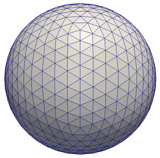
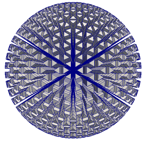
Figure 3: A visualisation of the “hedgehog” domain that is obtained by applying the mapping $\chi$ to a mesh of the spherical annulus constructed from columns of triangular prism elements. Top: the original domain $M^{\delta}$. Bottom: the transformed domain $\chi(M^{\delta})$.

Since our weak form of the equation only involves the divergence of test and trial functions, we can consider using H(div) elements for $V_{1}$, and discontinuous elements for $V_{2}$, chosen such that

$$\boldsymbol{u}^{\delta}\in V_{1}\implies\nabla\cdot\boldsymbol{u}^{\delta}\in V_{2},$$

which leads to a stable discretisation. In our test, we use the natural extension of Brezzi-Douglas-Marini (BDM) finite element spaces to triangular prisms, which we can express as

$$V_{1}=\operatorname{BDM}_{k}(\mbox{prism})=\begin{pmatrix}\operatorname{BDM}_{k}(\operatorname{triangle})\otimes\operatorname{DG}_{k-1}(\operatorname{interval})\\ \operatorname{DG}_{k-1}(\operatorname{triangle})\otimes\operatorname{CG}_{k}(\operatorname{interval})\\ \end{pmatrix},$$

where $\operatorname{DG}_{k}$ indicates a discontinuous finite element space of degree $k$, $\operatorname{CG}_{k}$ indicates a continuous finite element space of degree $k$, and $\otimes$ indicates a tensor product. Here the finite element space is described as a vector with the horizontal part of the vector fields above and the vertical part of the vector fields below. The finite element spaces are defined on the reference element $\hat{e}$ and transformed via the contravariant Piola transformation to obtain vector-valued functions in the physical elements in $\tilde{M}^{\delta}$ which are tangential to $\tilde{M}^{\delta}$, and have continuous normal components across element edges, by construction. This means that it is not necessary to include Lagrange multipliers to enforce the tangency constraint. Under the mapping $\chi:\tilde{M}^{\delta}\to\mathbb{R}^{3}$, we apply a further Piola transformation, which is equivalent to applying the Piola transformation from the reference element into the hedgehog mesh directly; this means that normal components of $\boldsymbol{u}^{\delta}$ are the same on either side of the jump between two neighbouring columns in $\chi(\tilde{M}^{\delta})$.

The corresponding discontinuous finite element space is

$$V_{2}=\operatorname{DG}_{k}(\mbox{prism})=\operatorname{DG}_{k-1}(\operatorname{triangle})\otimes\operatorname{DG}_{k-1}(\operatorname{interval}).$$

This pair of finite element spaces satisfies the Brezzi stability conditions with respect to our equations, and hence we expect convergence of numerical solutions at the optimal rate, provided that the spherical annulus domain is approximated at the correct order. Holst and Stern (2012) showed that this requires the correct order of convergence for not only the distance from the approximate to exact manifold in $\mathbb{R}^{4}$, but also the approximation of the normal direction to $\tilde{M}$. In the numerical calculations shown here, we used a piecewise linear description of the surface of the sphere, and hence we only expect first order convergence for $\boldsymbol{u}$, even if degree $k>1$ is chosen. As shown in Figure 4, we do indeed obtain first order convergence for $k=0$. For $k=1$, we obtain second order convergence for $h$ but only first order convergence for $\boldsymbol{u}$. This convergence demonstrates that our methodology produces convergent solutions under the shallow atmosphere approximation.

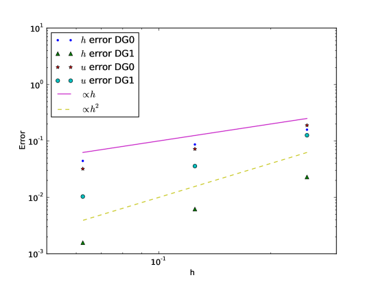
Figure 4: Plot showing errors in $h$ and $\boldsymbol{u}$ for $k=1$ and $k=2$. For $k=1$ we obtain first order convergence for both $h$ and $\boldsymbol{u}$. For $k=2$ we obtain secord order convergence for $h$ but sub-optimal convergence (somewhere between first and second order) for $\boldsymbol{u}$; this is because we have used a piecewise linear approximation to the annular domain.

5 Conclusions

In this paper we introduced a method for implementing the shallow atmosphere approximation with three dimensional finite element methods, by making use of a transformation from a three dimensional manifold embedded in $\mathbb{R}^{4}$. This can be implemented in a three dimensional finite element code by defining a transformation to a discontinuous coordinate field in $\mathbb{R}^{3}$. This methodology was demonstrated by numerical convergence tests for a prototype elliptic problem, implemented using the Firedrake software framework.

References

- Cotter and Shipton (2012) Cotter CJ, Shipton J. 2012. Mixed finite elements for numerical weather prediction. Journal of Computational Physics 231(21): 7076–7091.
- Dennis et al. (2011) Dennis J, Edwards J, Evans KJ, Guba O, Lauritzen PH, Mirin AA, St-Cyr A, Taylor MA, Worley PH. 2011. CAM-SE: A scalable spectral element dynamical core for the Community Atmosphere Model. International Journal of High Performance Computing Applications : 1094342011428 142.
- Holst and Stern (2012) Holst M, Stern A. 2012. Geometric variational crimes: Hilbert complexes, finite element exterior calculus, and problems on hypersurfaces. Foundations of Computational Mathematics 12(3): 263–293.
- Müller (1989) Müller R. 1989. A note on the relation between the “traditional approximation” and the metric of the primitive equations. Tellus A 41(2): 175–178.
- Nair et al. (2009) Nair R, Choi HW, Tufo H. 2009. Computational aspects of a scalable high-order discontinuous Galerkin atmospheric dynamical core. Computers & Fluids 38(2): 309–319.
- Phillips (1966) Phillips N. 1966. The equations of motion for a shallow rotating atmosphere and the “traditional approximation”. Journal of the atmospheric sciences 23(5): 626–628.
- Rognes et al. (2013) Rognes ME, Ham DA, Cotter CJ, McRae ATT. 2013. Automating the solution of PDEs on the sphere and other manifolds in FEniCS 1.2. Geoscientific Model Development 6(6): 2099–2119, doi:10.5194/gmd-6-2099-2013.
- Thuburn and White (2013) Thuburn J, White A. 2013. A geometrical view of the shallow-atmosphere approximation, with application to the semi-Lagrangian departure point calculation. Quarterly Journal of the Royal Meteorological Society 139(670): 261–268.
- Tort and Dubos (2014) Tort M, Dubos T. 2014. Dynamically consistent shallow-atmosphere equations with a complete Coriolis force. Quarterly Journal of the Royal Meteorological Society .
- Ullrich (2014) Ullrich PA. 2014. A global finite-element shallow-water model supporting continuous and discontinuous elements. Geoscientific Model Development Discussions 7(4): 5141–5182, doi:10.5194/gmdd-7-5141-2014.
- White et al. (2005) White AA, Hoskins BJ, Roulstone I, Staniforth A. 2005. Consistent approximate models of the global atmosphere: shallow, deep, hydrostatic, quasi-hydrostatic and non-hydrostatic. Quarterly Journal of the Royal Meteorological Society 131(609): 2081–2107.