Social Diffusion and Global Drift on Networks

Abstract

We study a mathematical model of social diffusion on a symmetric weighted network where individual nodes’ states gradually assimilate to local social norms made by their neighbors’ average states. Unlike physical diffusion, this process is not state conservational and thus the global state of the network (i.e., sum of node states) will drift. The asymptotic average node state will be the average of initial node states weighted by their strengths. Here we show that, while the global state is not conserved in this process, the inner product of strength and state vectors is conserved instead, and perfect positive correlation between node states and local averages of their self/neighbor strength ratios always results in upward (or at least neutral) global drift. We also show that the strength assortativity negatively affects the speed of homogenization. Based on these findings, we propose an adaptive link weight adjustment method to achieve the highest upward global drift by increasing the strength-state correlation. The effectiveness of the method was confirmed through numerical simulations and implications for real-world social applications are discussed.

I Introduction

Social contagion Christakis and Fowler (2013) has been studied in various contexts. Many instances of social contagion can be modeled as an infection process where a specific state (adoption of product, fad, knowledge, behavior, political opinion, etc.) spreads from individual to individual through links between them Van den Bulte and Stremersch (2004); Dodds and Watts (2004); Hill et al. (2010); Bond et al. (2012). In the meantime, other forms of social contagion may be better understood as a diffusion process where the state of an individual tends to assimilate gradually to the social norm (i.e., local average state) within his/her neighborhood Christakis and Fowler (2007); Fowler and Christakis (2008); Coronges et al. (2011); Coviello et al. (2014).

Unlike infection scenarios where influence is nonlinear, unidirectional, fast, and potentially disruptive, social diffusion is linear, bidirectional, gradual, and converging. The distance between an individual’s state and his/her neighbors’ average state always decreases, and thus a homogeneous global state is guaranteed to be the connected network’s stable equilibrium state in the long run Castellano et al. (2009).

Here, we focus on an unrecognized characteristic of social diffusion, i.e., non-trivial drift it can cause to the network’s global state. Although somewhat counterintuitive, such global drift is indeed possible because, unlike physical diffusion processes, social diffusion processes are not state conservational. In what follows, we study a simple mathematical model of social diffusion to understand the mechanisms of this process and obtain both asymptotic and instantaneous behaviors of the global state of the network. We also show how strength assortativity influences the speed of homogenization. Then we propose an adaptive network Gross and Sayama (2009) method of preferential link weight adjustment to achieve the highest upward global drift within a given time period. The relevance of social diffusion to individual and collective improvement is discussed, with a particular emphasis on educational applications.

II Mathematical Model of Social Diffusion

Let us begin with the conventional physical diffusion equation on a simple symmetric network,

$$\frac{ds}{dt}=-cLs,$$ (1)

where $s$ is the node state vector of the network, $c$ the diffusion constant, and $L$ the Laplacian matrix of the network. The Laplacian matrix of a network is defined as $L=D-A$, where $A$ is the adjacency matrix of the network and $D$ is a diagonal matrix of the nodes’ degrees. If the network is connected, the coefficient matrix $(-cL)$ has one and only one dominant eigenvalue, $\lambda_{0}=0$, whose corresponding eigenvector is the homogeneity vector $h=(1\;1\;1\;\ldots\;1)^{T}$. Therefore, the solutions of this equation always converge to a homogeneous state regardless of initial conditions if the network is connected. It is easy to show that this process is state conservational, i.e., the sum (or, equivalently, average) of node states, $h^{T}s$, will not change over time:

$$\frac{d(h^{T}s)}{dt}=-ch^{T}Ls=-c(Lh)^{T}s=0$$ (2)

This indicates that no drift of the global state is possible in physical diffusion processes on a simple symmetric network.

Social diffusion processes can be modeled differently. In this scenario, a state of an individual node may represent any quantitative property of the individual that is subject to social influence from his/her peers, such as personal preference, feeling, cooperativeness, etc. We assume that each individual gradually assimilates his/her state to the social norm around him/her. The dynamical equation of social diffusion can be written individually as

$$\frac{ds_{i}}{dt}=c\left(\langle s_{j}\rangle^{i}_{j}-s_{i}\right),$$ (3)

where $s_{i}$ is the state of individual $i$, and $\langle x_{j}\rangle^{i}_{j}$ is a local weighted average of $x_{j}$ around individual $i$, i.e.,

$$\langle x_{j}\rangle^{i}_{j}=\frac{\sum_{j}a_{ij}x_{j}}{\sum_{j}a_{ij}},$$ (4)

with $a_{ij}\geq 0$ being the connection weight from individual $j$ to individual $i$. In Eq. (3) $x_{j}=s_{j}$, but this weighted averaging will also be used for other local quantities later in this paper. We note that Eq. (4) carries a dummy variable $j$ outside the brackets. While not customary, such explicit specification of dummy variable $j$ is necessary in the present study, in order to disambiguate which index the averaging is conducted over when calculating nested local averages (to appear later).

$\langle s_{j}\rangle^{i}_{j}$ in Eq. (3) represents the social norm for individual $i$. Discrete-time versions of similar models are also used to describe peer effects in opinion dynamics in sociology Friedkin and Johnsen (1990), distributed consensus formation (called “agreement algorithms”) in control and systems engineering Bertsekas and Tsitsiklis (1989); Blondel et al. (2005); Lambiotte et al. (2011), and for statistical modeling of empirical social media data more recently Coviello et al. (2014).

In this paper, we focus on symmetric interactions between individuals (i.e., $a_{ij}=a_{ji}$). Such symmetry is a reasonable assumption as a model of various real-world collaborative or contact relationships, e.g., networks of coworkers in an organization, networks of students in a school, and networks of residents in a community, to which symmetric social interaction can be relevant. Self-loops are allowed in our model, i.e., $a_{ii}$ may be non-zero. Such self-loops represent self-confidence of individuals when calculating their local social norms. The sum of weights of all links attached to a node $i$, $k_{i}=\sum_{j}a_{ij}=\sum_{j}a_{ji}$, is called the strength of node $i$ Barrat et al. (2004), which would correspond to a node degree for unweighted networks. This social diffusion model requires $k_{i}\neq 0$ $\forall i$; otherwise Eq. (4) would be indeterminate and there would be no meaningful dynamics to be described for the individual.

Eq. (3) can be rewritten at a collective level as

$$\frac{ds}{dt}=c(D^{-1}A-I)s,$$ (5)

where $A=(a_{ij})$ and $D^{-1}$ is a square matrix whose $i$-th diagonal component is $k_{i}^{-1}$ while non-diagonal components are all zero. If the network does not have link weights or self-loops (i.e., $a_{ij}\in\{0,1\}$, $a_{ii}=0$), $D^{-1}$ and $A$ are conventional inverse degree and adjacency matrices, respectively, and thus the matrix $D^{-1}A-I=-D^{-1}L$ is a special case of the coupling matrix discussed in Motter et al. (2005), with scaling exponent 1 and a negative sign added.

III Asymptotic Behaviors

Eq. (5) is essentially the same as Eq. (1) if the network is regular without link weights or self-loops (i.e., $a_{ij}\in\{0,1\}$, $a_{ii}=0$, $k_{i}=k$ $\forall i$). Even if not regular, it is still a simple matrix differential equation, for which a general solution is always available. If the network is connected, the coefficient matrix $c(D^{-1}A-I)$ has one and only one dominant eigenvalue 0 with corresponding eigenvector $h$, hence the state of the network will always converge to a homogeneous equilibrium state, just like in the physical diffusion equation. Hence the asymptotic state can be written as

$$s_{\infty}=\lim_{t\to\infty}s(t)=\langle s_{\infty}\rangle h,$$ (6)

where $\langle s_{\infty}\rangle$ is the average node state in $s_{\infty}$.

It is known that a discrete time version of Eq. (5) will converge to a weighted average of initial node states with their strengths used as weights, if the network is connected and non-bipartite Lambiotte et al. (2011). The same conclusion was also reported for the ensemble average of the voter model with a node-update scheme Suchecki et al. (2005). It can be easily shown that our continuous-time model has the same asymptotic state, as follows.

First, we show that the inner product of strength and state vectors, $g^{T}s$ with $g=(k_{1}\;k_{2}\;\ldots\;k_{n})^{T}$ (where $n$ is the number of individuals), is always conserved instead of node states during social diffusion on a symmetric network, because

$$\frac{d(g^{T}s)}{dt}=cg^{T}D^{-1}As-cg^{T}s=ch^{T}As-cg^{T}s=0.$$ (7)

This holds for any symmetric networks regardless of their topologies and link weights. We call $g^{T}s$ a strength-state product hereafter.

This conservation law was already known for the ensemble average of the node-update voter model Suchecki et al. (2005), and the existence of similar conservation laws was also shown for more generalized voter-like models with directed links Serrano et al. (2009). Our result above provides an example of the same conservation law realized in a different model setting, i.e., continuous-time/state social diffusion models on weighted, undirected networks.

Calculating an inner product of each side of Eq. (6) with $g$ makes

$$g^{T}s_{\infty}=\langle s_{\infty}\rangle g^{T}h.$$ (8)

The conservation of the strength-state product (Eq. (7)) allows us to replace the left hand side, resulting in

$$g^{T}s_{0} = \langle s_{\infty}\rangle g^{T}h,$$ (9)

$$\langle s_{\infty}\rangle = g^{T}s_{0}/g^{T}h$$ (10)

$$= (k_{1}/K\;k_{2}/K\;\ldots\;k_{n}/K)^{T}s_{0},$$ (11)

where $K=g^{T}h=\sum_{i}k_{i}$. This shows that the asymptotic average node state is a weighted average of initial node states where their strengths are used as weights.

In discrete-time distributed consensus formation models, the network needs to be non-bipartite (in addition to being connected) for global homogenization to be reached Lambiotte et al. (2011), but the model discussed here does not require non-bipartiteness because time is continuous.

The overall net gain or loss of the global state that can be attained asymptotically by social diffusion is calculated as

$$\Delta_{\infty} = h^{T}s_{\infty}-h^{T}s_{0}$$ (12)

$$= h^{T}\left(\frac{g^{T}s_{0}}{g^{T}h}h\right)-h^{T}s_{0}$$ (13)

$$= (\hat{g}-h)^{T}s_{0},$$ (14)

where $\hat{g}=g/\langle k\rangle$ with $\langle k\rangle=g^{T}h/n$ (i.e., average strength). This means that the asymptotic net gain or loss will be determined by the correlation between the initial state vector $s_{0}$ and another vector $(\hat{g}-h)$ that is determined by the node strengths.

IV Instantaneous Behaviors

Next, we study the instantaneous direction of drift of the global state (sum of node states, $h^{T}s$), which can be written as

$$\frac{d(h^{T}s)}{dt} = ch^{T}(D^{-1}A-I)s$$ (15)

$$= c(w^{T}s)-c(h^{T}s),$$ (16)

where $w=AD^{-1}h$. $w$ can be further detailed as

$$w=\left(\begin{array}[]{c}\sum_{j}a_{1j}k_{j}^{-1}\\ \sum_{j}a_{2j}k_{j}^{-1}\\ \vdots\\ \sum_{j}a_{nj}k_{j}^{-1}\\ \end{array}\right)\\ =\left(\begin{array}[]{c}\langle k_{1}/k_{j}\rangle^{1}_{j}\\ \langle k_{2}/k_{j}\rangle^{2}_{j}\\ \vdots\\ \langle k_{n}/k_{j}\rangle^{n}_{j}\\ \end{array}\right).$$ (17)

Each component of $w$ is the local average of self/neighbor strength ratios, $k_{i}/k_{j}$, which tends to be greater than 1 if the individual has more connection weights than its neighbors, or less than 1 otherwise (but always strictly positive). In this regard, $w$ characterizes the local strength differences for all individuals in society. If $(w-h)^{T}s>0$, the global state will drift upward due to social diffusion. Also note that $w^{T}h=n$, because

$$w^{T}h = \sum_{i}\sum_{j}a_{ij}k_{j}^{-1}$$ (18)

$$= \sum_{j}\left(k_{j}^{-1}\sum_{i}a_{ij}\right)=\sum_{j}k_{j}^{-1}k_{j}=n.$$ (19)

We show $w\approx\hat{g}$ for networks with neutral strength assortativity (called non-assortative networks hereafter). Let $P(k^{\prime}|k)$ be the conditional probability density for a link originating from a $k$-degree node to reach a $k^{\prime}$-degree node. Then, each component of $w$ in Eq. (17) is approximated as

$$\langle k_{i}/k_{j}\rangle^{i}_{j}\approx k_{i}\int_{k^{\prime}}k^{\prime-1}P(k^{\prime}|k_{i})dk^{\prime}.$$ (20)

For non-assortative networks, $P(k^{\prime}|k_{i})$ does not depend on $k_{i}$ Barabási (012):

$$P(k^{\prime}|k_{i})=k^{\prime}P(k^{\prime})/\int_{k^{\prime}}k^{\prime}P(k^{\prime})dk^{\prime}=k^{\prime}P(k^{\prime})/\langle k\rangle$$ (21)

Applying Eq. (21) to Eq. (20) makes

$$\langle k_{i}/k_{j}\rangle^{i}_{j}\approx k_{i}\int_{k^{\prime}}k^{\prime-1}k^{\prime}P(k^{\prime})dk^{\prime}/\langle k\rangle=k_{i}/\langle k\rangle.$$ (22)

With this, Eq. (17) is approximated as

$$w\approx g/\langle k\rangle=\hat{g}.$$ (23)

Using $\hat{g}$, we obtain the following approximated dynamical equation for non-assortative networks, which is quite similar to Eq. (14):

$$\frac{d(h^{T}s)}{dt}\approx c(\hat{g}^{T}s)-c(h^{T}s)=c(\hat{g}-h)^{T}s$$ (24)

Furthermore, we prove that perfect positive correlation between node states ($s$) and local averages of their self/neighbor strength ratios ($w$) always results in upward (or at least neutral) global drift. If those two vectors are in perfect positive correlation, $s=\alpha w$ with positive constant $\alpha$. Then Eq. (16) becomes

$$\frac{d(h^{T}s)}{dt}=\alpha c(w-h)^{T}w.$$ (25)

Here, $w$ and $w-h$ are the hypotenuse and adjacent of a right triangle in an $n$-dimensional state space, respectively, because

$$(w-h)^{T}h=w^{T}h-h^{T}h=n-n=0,$$ (26)

which shows $(w-h)\perp h$. Therefore, the angle between $(w-h)$ and $w$ cannot be greater than $\pi/2$, which guarantees in Eq. (25) that $d(h^{T}s)/dt$ is always non-negative. Figure 1 visually illustrates the relationships between the vectors discussed above.

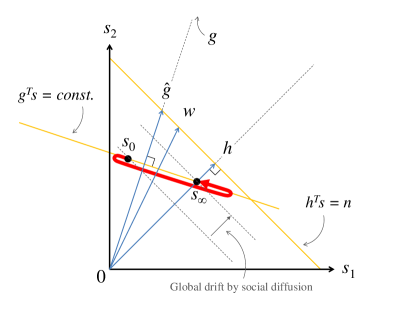
Figure 1: (Color online) Visual illustration of the relationships between several vectors discussed ($h$, $w$, $g$, $\hat{g}$, $s_{0}$, $s_{\infty}$). This diagram is drawn in two dimensions for simplicity, but the actual vectors exist in an $n$-dimensional state space. Note that $h^{T}h=w^{T}h=\hat{g}^{T}h=n$. If the network is non-assortative, then $w\approx\hat{g}$.

V Approximation as Low-Dimensional Linear Dynamical System and Analysis of Homogenization Speed

Here we analyze the speed of homogenization caused by social diffusion on networks by approximating the whole dynamics in a low-dimensional linear dynamical system about $h^{T}s$ and $w^{T}s$. The dynamics of $w^{T}s$ is given by

$$\frac{d(w^{T}s)}{dt} = cw^{T}D^{-1}(A-D)s$$ (27)

$$= c(u^{T}s)-c(w^{T}s),$$ (28)

where $u=AD^{-1}w$, which is further detailed as

$$u=A\left(\begin{array}[]{c}\langle k_{j}^{-1}\rangle^{1}_{j}\\ \langle k_{j}^{-1}\rangle^{2}_{j}\\ \vdots\\ \langle k_{j}^{-1}\rangle^{n}_{j}\\ \end{array}\right)=\left(\begin{array}[]{c}\langle\langle k_{1}/k_{j}\rangle^{i}_{j}\rangle^{1}_{i}\\ \langle\langle k_{2}/k_{j}\rangle^{i}_{j}\rangle^{2}_{i}\\ \vdots\\ \langle\langle k_{n}/k_{j}\rangle^{i}_{j}\rangle^{n}_{i}\\ \end{array}\right).$$ (29)

If we can approximate $u$ using $h$ and/or $w$, the system closes and a simple eigenvalue analysis reveals the speed of homogenization.

For non-assortative networks, the approximation in Eq. (22) gives

$$u\approx g/\langle k\rangle=\hat{g}.$$ (30)

Combining this with Eq. (23), we obtain

$$\frac{d(w^{T}s)}{dt}\approx c(\hat{g}^{T}s)-c(\hat{g}^{T}s)=0,$$ (31)

which is consistent with our analyses derived earlier. Combining this result with Eq. (16) makes the following two-dimensional linear dynamical system:

$$\frac{d}{dt}\begin{pmatrix}h^{T}s\\ w^{T}s\end{pmatrix}=c\left(\begin{array}[]{rr}-1&1\\ 0&0\end{array}\right)\begin{pmatrix}h^{T}s\\ w^{T}s\end{pmatrix}$$ (32)

The coefficient matrix above has eigenvalues $0$ and $-c$ with corresponding eigenvectors $(1\;1)^{T}$ and $(1\;0)^{T}$, respectively. The second eigenvalue ($-c$) represents the baseline speed of homogenization on non-assortative networks.

This low-dimensional dynamical systems approach can be extended to networks with negative or positive strength assortativity. In so doing, we adopt a scaling model Gallos et al. (2008); Barabási (012) to approximate the strength of a neighbor of node $i$ by a scaling function of $k_{i}$,

$$k_{j}\approx bk_{i}^{\mu},$$ (33)

where $\mu$ is the correlation exponent and $b$ is a positive constant. Applying this approximation to Eq. (29) gives

$$u \approx \left(\begin{array}[]{c}k_{1}/(b(bk_{1}^{\mu})^{\mu})\\ k_{2}/(b(bk_{2}^{\mu})^{\mu})\\ \vdots\\ k_{n}/(b(bk_{n}^{\mu})^{\mu})\\ \end{array}\right)=b^{-1-\mu}\left(\begin{array}[]{c}k_{1}^{1-\mu^{2}}\\ k_{2}^{1-\mu^{2}}\\ \vdots\\ k_{n}^{1-\mu^{2}}\\ \end{array}\right).$$ (42)

This approximation indicates that, if $\mu\to 0$, $u\to g/b$, which agrees with Eq. (30) for non-assortative networks. For simplicity, we limit our analysis to two unrealistic yet illustrative cases with $\mu=\pm 1$, because this setting makes $1-\mu^{2}=0$ with which the dynamics can still be written using $h$ and $w$ only.

For strongly disassortative networks ($\mu=-1$), Eq. (42) becomes $u\approx h$. The resulting linear dynamical system is

$$\frac{d}{dt}\begin{pmatrix}h^{T}s\\ w^{T}s\end{pmatrix}=c\left(\begin{array}[]{rr}-1&1\\ 1&-1\end{array}\right)\begin{pmatrix}h^{T}s\\ w^{T}s\end{pmatrix},$$ (43)

whose coefficient matrix has eigenvalues $0$ and $-2c$ with corresponding eigenvectors $(1\;1)^{T}$ and $(-1\;1)^{T}$, respectively. The second eigenvalue ($-2c$) is smaller than that of non-assortative networks, which shows that the homogenization takes place faster on disassortative networks.

Finally, for strongly assortative networks ($\mu=1$), applying the approximation Eq. (33) with $\mu=1$ to Eq. (17) gives $w\approx h/b$, and also Eq. (42) gives $u\approx h/b^{2}$. This means that the system is essentially collapsed into the following one-dimensional linear dynamical system:

$$\frac{d(h^{T}s)}{dt} = c((h/b)^{T}s)-c(h^{T}s)$$ (44)

$$= -c\frac{b-1}{b}(h^{T}s)$$ (45)

For any positive $b$ and $c$, always

$$-c\frac{b-1}{b}>-c.$$ (46)

This shows that the homogenization takes place slower on assortative networks than on non-assortative networks. Moreover, if the network is truly strongly assortative, $b$ must be close to 1 by definition. This brings the coefficient in Eq. (45) close to 0. Therefore the homogenization process on a strongly assortative network must be extremely slow. This can also be understood intuitively; extreme assortativity would result in having links only between nodes of equal strength, making the network disconnected and thus stopping the homogenization process.

These analytical results collectively illustrate that, as the strength assortativity increases, the speed of homogenization goes down. This finding is consistent with the negative effect of degree assortativity on the spectral gap of the Laplacian matrix reported in Van Mieghem et al. (2010) and on entropy measures of biased random walks reported in Sinatra et al. (2011), and also similar to the enhancement of synchronizability of networked nonlinear oscillators by negative degree assortativity Sorrentino et al. (2006); di Bernardo et al. (2007); Arenas et al. (2008).

We conducted numerical simulations of social diffusion on random and scale-free networks with non-assortative, disassortative and assortative topologies. The results are shown in Fig. 2. While the simulated networks did not have correlation exponents as extreme as $\mu=\pm 1$ assumed in the analysis above, the simulation results agree with the analytical predictions, especially during the initial time period when the networks tend to show a significant global drift on non-assortative and disassortative networks.

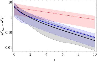
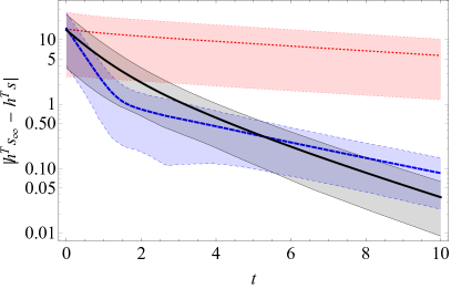
(a) random	(b) scale-free

  : non-assortative networks                                 : disassortative networks                                       : assortative networks

Figure 2: (Color online) Time evolution of the global state $h^{T}s$ toward the asymptotic state $h^{T}s_{\infty}$ during social diffusion on networks. The absolute difference between $h^{T}s$ and $h^{T}s_{\infty}$ is plotted over time. Black solid, blue dashed, and pink dotted curves show results with non-assortative, disassortative and assortative topologies, respectively. Each curve shows the mean of 100 independent numerical simulation runs, with shaded areas representing standard deviations. Each simulation was conducted using Eq. (3), starting with a randomly generated initial condition with $n=1,000$, $c=1$, node state range $[-1,1]$ and link weight range $[0,10]$. Numerical integration was conducted for $t=0\sim 10$ using a simple Euler forward method with step size $\delta t=0.01$. (a): Results on random networks. (b): Results on scale-free networks. Network topologies were generated first as an unweighted network by using the Erdős-Rényi (for random) or Barabási-Albert (for scale-free) network generation algorithm. Disconnected networks were not used for the experiment. Self-loops were randomly added to nodes with 1% probability. Once the topology was generated, a random link weight was assigned to each link. For assortative/disassortative networks, a revised Xulvi-Brunet & Sokolov algorithm Xulvi-Brunet and Sokolov (2004); Barabási (012) was additionally used to tune their strength assortativity. Assortative (or disassortative) network topologies were created by applying to a randomly generated non-assortative network 30,000 times of possible link rewirings that would enhance degree assortativity (or disassortativity) while preserving node degrees. Any link rewiring that would disconnect the network or create a multi-link was forbidden. Self-loops were allowed in the above operations. Every time a new link was created between originally disconnected nodes, a random link weight was assigned to the new link.

VI Adaptive Link Weight Adjustment to Promote Upward Global Drift

The analytical results presented above suggest that, if the local averages of people’s self/neighbor strength ratios are positively correlated with their states and if the network’s strength assortativity is negative, then an upward drift of the global state will occur quickly.

Here, we propose an adaptive network Gross and Sayama (2009) method of preferential link weight adjustment based on node states and strengths in order to promote upward global drift while social diffusion is ongoing. Specifically, we let each pair of nodes $i$ and $j$ dynamically change their connection weight $a_{ij}$ according to the following dynamical equation,

$$\frac{da_{ij}}{dt}=a_{ij}\left(\alpha\frac{s_{i}+s_{j}-2\langle s\rangle}{2\sigma_{s}}-\beta\frac{(k_{i}-\langle k\rangle)(k_{j}-\langle k\rangle)}{\sigma_{k}^{2}}\right),$$ (47)

where $\sigma_{s}$ and $\sigma_{k}$ are the standard deviations of node states and link weights, respectively. The first term inside the parentheses represents the change of link weights to induce positive correlation between node states and strengths (which naturally promotes positive correlation between node states and local averages of their self/neighbor strength ratios), while the second one is to induce negative strength assortativity.

We examined the effectiveness of this method for promotion of upward global drift through numerical simulations starting with an initially random or scale-free network topology with no prior strength-state correlation or strength assortativity. Systematic simulations were conducted with $\alpha$ and $\beta$ varied logarithmically. Results are shown in Fig. 3. It was found that the induction of positive strength-state correlation ($\alpha>0$) significantly promoted upward global drift. In the meantime, the induction of negative strength assortativity ($\beta>0$) increased the variability of outcomes but did not have a substantial influence on the direction of the global drift. The highest upward global drift was achieved when $\alpha$ was large and $\beta$ was small, i.e., when adaptive link weight adjustment was used merely for inducing positive strength-state correlation but not for inducing negative strength assortativity.

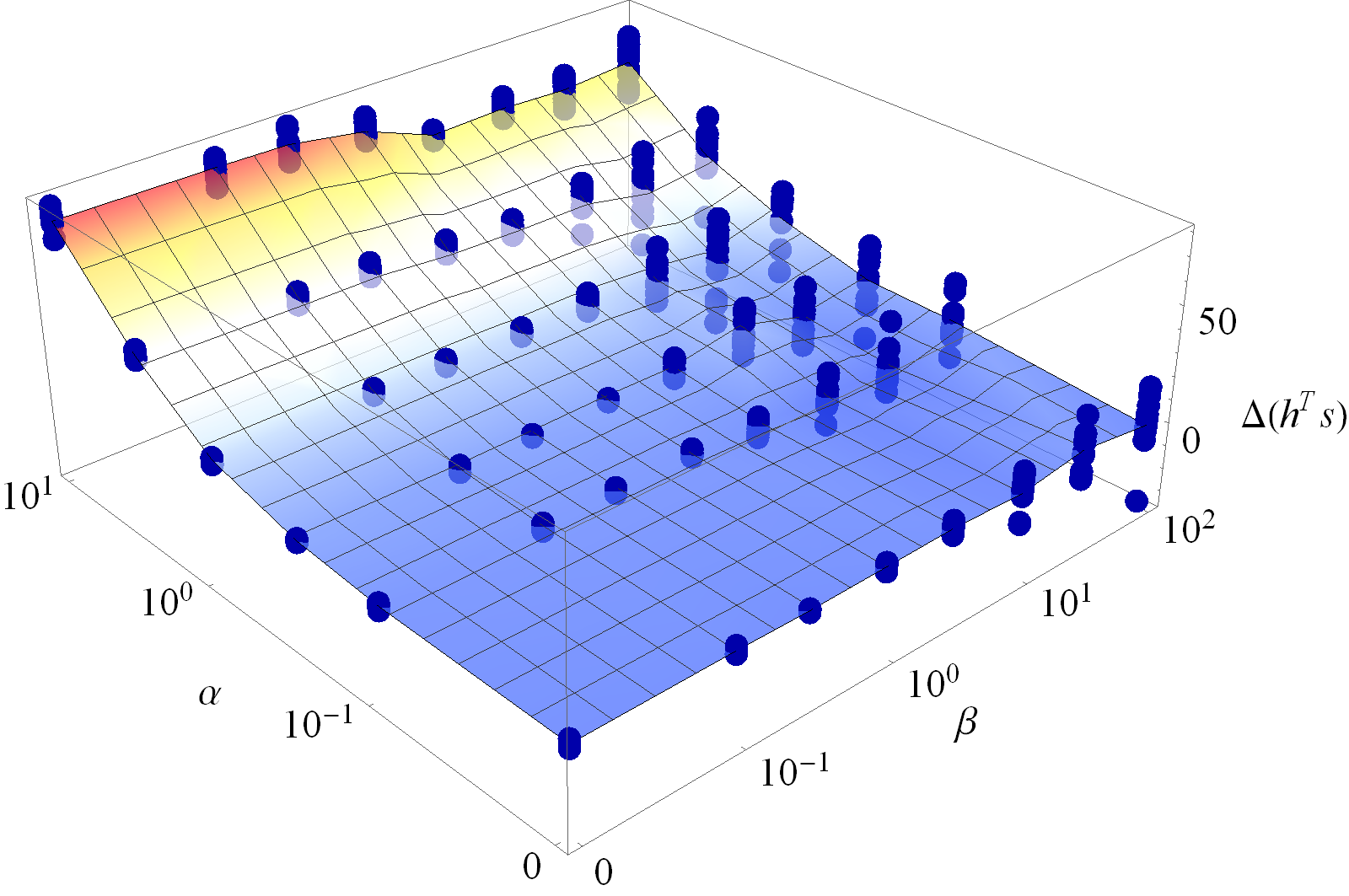
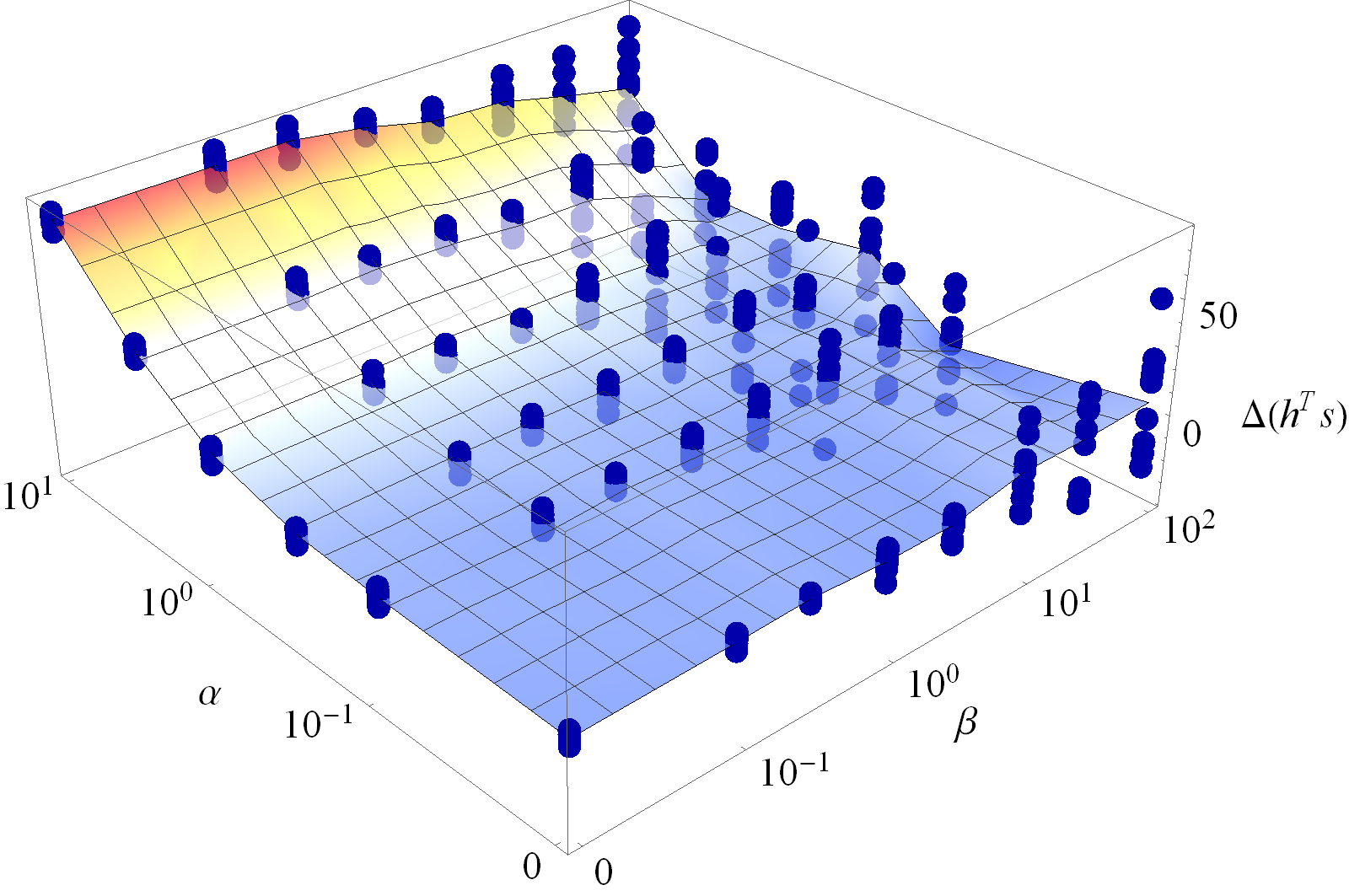
(a) (initially) random	(b) (initially) scale-free

Figure 3: (Color online) Summary of systematic simulations of social diffusion with adaptive link weight adjustment with logarithmically varied $\alpha$ and $\beta$ (cases with $\alpha=0$ or $\beta=0$ are also added to the lower ends of the axes). The difference in the global state between before and after each simulation ($\Delta h^{T}s$) is plotted over the $\alpha$-$\beta$ parameter space. Ten independent simulation runs were conducted for each parameter setting. Each dot represents one simulation run, while the surface shows the trend of the average. The initial network topology was generated using the Erdős-Rényi (a) or Barabási-Albert (b) network generation algorithm, each with 200 nodes and 20% connection density. Node states and link weights were initially random in the same way as in the previous experiment (Fig. 2). $c=1$. Numerical integration was conducted for $t=0\sim 1$ using a simple Euler forward method with step size $\delta t=0.01$.

VII Conclusions

In this paper, we studied the drift of the global state of a network caused by social diffusion. We showed that the inner product of strength and state vectors is a conserved quantity in social diffusion, which plays an essential role in determining the direction and asymptotic behavior of the global drift. We also showed both analytically and numerically that the strength assortativity of network topology has a negative effect on the speed of homogenization. We numerically demonstrated that manipulation of strength-state correlation via adaptive link weight adjustment effectively promoted upward drift of the global state.

This study has illustrated the possibility that social diffusion may be exploited for individual and collective improvement in real-world social networks. Mechanisms like the adaptive link weight adjustment used in the simulations above may be utilized in practice to, for example, help spread desirable behaviors and/or suppress undesirable behaviors among youths.

One particularly interesting application area of social diffusion is education. We have studied possible social diffusion of academic success in high school students’ social network Blansky et al. (2013). This naturally led educators to ask how one could utilize such diffusion dynamics to improve the students’ success at a whole school level. Naïve mixing of students may not be a good strategy due to bidirectional effects of social diffusion. Our results suggest that carefully inducing correlation between strengths (amount of social contacts) and states (academic achievements) would be a promising, implementable practice at school by, e.g., allowing higher-achieving students to participate in more extracurricular activities.

The work presented in this paper still has several limitations that will require further study. We have so far considered simple symmetric networks only, but social diffusion can take place on asymmetric, weighted social networks as well. Our analysis of assortative/disassortative network cases used unrealistic extreme assumptions ($\mu=\pm 1$) and ignored topological constraints such as structural cutoffs that are inevitable for assortative cases Barabási (012). Further exploration in these fronts will be necessary to obtain more generalizable understanding of the social diffusion dynamics on more complex real-world networks.

References

- Christakis and Fowler (2013) N. A. Christakis and J. H. Fowler, Statistics in medicine 32, 556 (2013).
- Van den Bulte and Stremersch (2004) C. Van den Bulte and S. Stremersch, Marketing Science 23, 530 (2004).
- Dodds and Watts (2004) P. S. Dodds and D. J. Watts, Physical Review Letters 92, 218701 (2004).
- Hill et al. (2010) A. L. Hill, D. G. Rand, M. A. Nowak, and N. A. Christakis, PLOS Computational Biology 6, e1000968 (2010).
- Bond et al. (2012) R. M. Bond, C. J. Fariss, J. J. Jones, A. D. Kramer, C. Marlow, J. E. Settle, and J. H. Fowler, Nature 489, 295 (2012).
- Christakis and Fowler (2007) N. A. Christakis and J. H. Fowler, New England Journal of Medicine 357, 370 (2007).
- Fowler and Christakis (2008) J. H. Fowler and N. A. Christakis, BMJ: British Medical Journal 337 (2008).
- Coronges et al. (2011) K. Coronges, A. W. Stacy, and T. W. Valente, Addictive Behaviors 36, 1305 (2011).
- Coviello et al. (2014) L. Coviello, Y. Sohn, A. D. Kramer, C. Marlow, M. Franceschetti, N. A. Christakis, and J. H. Fowler, PloS one 9, e90315 (2014).
- Castellano et al. (2009) C. Castellano, S. Fortunato, and V. Loreto, Reviews of modern physics 81, 591 (2009).
- Gross and Sayama (2009) T. Gross and H. Sayama, Adaptive Networks (Springer, 2009).
- Friedkin and Johnsen (1990) N. E. Friedkin and E. C. Johnsen, Journal of Mathematical Sociology 15, 193 (1990).
- Bertsekas and Tsitsiklis (1989) D. P. Bertsekas and J. N. Tsitsiklis, “Parallel and distributed computation: numerical methods,” (Prentice-Hall, Inc., 1989) Chap. 7.3.
- Blondel et al. (2005) V. Blondel, J. M. Hendrickx, A. Olshevsky, J. Tsitsiklis, et al., in IEEE Conference on Decision and Control, Vol. 44 (IEEE; 1998, 2005) p. 2996.
- Lambiotte et al. (2011) R. Lambiotte, R. Sinatra, J.-C. Delvenne, T. Evans, M. Barahona, and V. Latora, Physical Review E 84, 017102 (2011).
- Barrat et al. (2004) A. Barrat, M. Barthelemy, R. Pastor-Satorras, and A. Vespignani, Proceedings of the National Academy of Sciences of the United States of America 101, 3747 (2004).
- Motter et al. (2005) A. E. Motter, C. Zhou, and J. Kurths, Physical Review E 71, 016116 (2005).
- Suchecki et al. (2005) K. Suchecki, V. M. Eguiluz, and M. San Miguel, Europhysics Letters 69, 228 (2005).
- Serrano et al. (2009) M. A. Serrano, K. Klemm, F. Vazquez, V. M. Eguíluz, and M. San Miguel, Journal of Statistical Mechanics: Theory and Experiment 2009, P10024 (2009).
- Barabási (012 ) A.-L. Barabási, “Network science book,” (Center for Complex Network Research, Northeastern University, 2012-) Chap. 7. Degree Correlations, available at http://barabasilab.neu.edu/networksciencebook/.
- Gallos et al. (2008) L. K. Gallos, C. Song, and H. A. Makse, Physical review letters 100, 248701 (2008).
- Van Mieghem et al. (2010) P. Van Mieghem, H. Wang, X. Ge, S. Tang, and F. Kuipers, The European Physical Journal B-Condensed Matter and Complex Systems 76, 643 (2010).
- Sinatra et al. (2011) R. Sinatra, J. Gómez-Gardeñes, R. Lambiotte, V. Nicosia, and V. Latora, Physical Review E 83, 030103 (2011).
- Sorrentino et al. (2006) F. Sorrentino, M. Di Bernardo, G. H. Cuellar, and S. Boccaletti, Physica D: nonlinear phenomena 224, 123 (2006).
- di Bernardo et al. (2007) M. di Bernardo, F. Garofalo, and F. Sorrentino, International Journal of Bifurcation and Chaos 17, 3499 (2007).
- Arenas et al. (2008) A. Arenas, A. Díaz-Guilera, J. Kurths, Y. Moreno, and C. Zhou, Physics Reports 469, 93 (2008).
- Xulvi-Brunet and Sokolov (2004) R. Xulvi-Brunet and I. M. Sokolov, Physical Review E 70, 066102 (2004).
- Blansky et al. (2013) D. Blansky, C. Kavanaugh, C. Boothroyd, B. Benson, J. Gallagher, J. Endress, and H. Sayama, PLOS ONE 8, e55944 (2013).