A numerical approach for the Poisson equation
in a planar domain with a small inclusion

Lucas Chesnel¹, Xavier Claeys^2
1 Centre de math matiques appliqu es, École Polytechnique, 91128 Palaiseau, France;
² Laboratoire Jacques-Louis Lions, Université Pierre et Marie Curie, 4 place Jussieu, 75005 Paris, France.
E-mail: lucas.chesnel@cmap.polytechnique.fr, claeys@ann.jussieu.fr
(March 15, 2024)

Abstract. We consider the Poisson equation in a domain with a small hole of size $\delta$. We present a simple numerical method, based on an asymptotic analysis, which allows to approximate robustly the far field of the solution as $\delta$ goes to zero without meshing the small hole. We prove the stability of the scheme and provide error estimates. We end the paper with numerical experiments illustrating the efficiency of the technique.

Key words. Small hole, asymptotic analysis, singular perturbation, finite element method.

1 Introduction

In the present article, we consider $\omega,\Omega\subset\mathbb{R}^{2}$ two bounded Lipschitz domains such that $\overline{\omega}\subset\Omega$. Define $\omega_{\delta}:=\{\boldsymbol{x}\in\mathbb{R}^{2},\;\boldsymbol{x}/\delta\in\omega\}$ and $\Omega_{\delta}:=\Omega\setminus\overline{\omega}_{\delta}$. Given a data $f\in\mathrm{L}^{2}(\Omega)$, we are interested in devising a robust and accurate numerical method for approximating, for small values of $\delta$, the far field of the function satisfying

$$u_{\delta}\in\mathrm{H}^{1}_{0}(\Omega_{\delta})\quad\textrm{ and }\quad-\Delta u_{\delta}=f\quad\textrm{in}\;\Omega_{\delta}.$$ (1)

In (1), $\mathrm{H}^{1}_{0}(\Omega_{\delta})$ denotes the subspace of the elements of the Sobolev space $\mathrm{H}^{1}(\Omega_{\delta})$ vanishing on $\partial\Omega_{\delta}$. On the other hand, we call far field of $u_{\delta}$ the restriction of $u_{\delta}$ to $\Omega\setminus\overline{\mathrm{D}}_{r}$, where $\mathrm{D}_{r}:=\mathrm{D}(0,r)$ is the disk with fixed arbitrary radius $r>0$. Problem (1), or variants of it, arises as a simple but relevant model in many applications ranging from electrical engineering [5, 37] to flow transport around wells [14, 36]. This kind of problem also appears when considering wave scattering by small impenetrable inclusions [13].

In order to solve numerically Problem (1), a crude but rather natural idea would consist in neglecting the influence of the small inclusion on the total field $u_{\delta}$. Indeed (see for example [31]), as $\delta\to 0$ the function $u_{\delta}$ converges toward $u_{0}$ the solution to the limit problem where the inclusion has disappeared

$$u_{0}\in\mathrm{H}^{1}_{0}(\Omega)\quad\textrm{ and }\quad-\Delta u_{0}=f\quad\textrm{in}\;\Omega.$$ (2)

However, in the general case (more precisely, when $u_{0}(0)\neq 0$), the convergence turns out to be very slow: for any arbitrary radius $r>0$ such that $\overline{\mathrm{D}}_{r}\subset\Omega$, we have $\|u_{\delta}-u_{0}\|_{\mathrm{H}^{1}(\Omega\setminus\overline{\mathrm{D}}_{r})}\geq\,C\,|\ln\delta|^{-1}\|f\|_{\mathrm{L}^{2}(\Omega)}$, for some constant $C>0$ independent of $\delta$. To give an idea $|\ln\delta|^{-1}\approx 0.0434$ for $\delta=10^{-10}$. Thus, neglecting the presence of the small inclusion is not satisfactory from a computational point of view, and a reasonable numerical approach for (1) should reproduce accurately the perturbation induced by the presence of the small inclusion $\omega_{\delta}$.

Most of the numerical approaches that could be considered for dealing with this problem suffer from a numerical locking effect [2]: performances of standard strategies deteriorate as $\delta\to 0$. Admittedly, robust strategies already exist in the literature, like the multi-scale finite element method coupled with some mesh refinement strategy [22], or the boundary element method (see e.g. [1]). These techniques provide satisfying results in many cases, but they require careful and thorough implementation efforts, and/or rely on strong assumptions such as homogeneity of the coefficients of the equation under consideration. Other numerical strategies are based on an approximation of $u_{\delta}$ of the form "$u_{0}$ + corrector", where both terms of this sum are computed separately (see for example [18, 7]). These approaches may induce substantial additional computational cost in a real life simulation. In many practical situations, small inclusions are not the main subject of concern, and it would be desirable to devise a simple, general purpose and implementation friendly method that would not rely on any kind of mesh refinement technique, while remaining robust as $\delta\to 0$. This is the purpose of the present article to describe and analyse a method matching these requirements, while relying on only one numerical resolution.

The outline of this article is the following. In Section 2, we summarize the main results concerning the asymptotic expansion of $u_{\delta}$ with respect to the size of the small hole. Section 3 is dedicated to the construction of a model problem, based on the matched expansion of $u_{\delta}$, whose solution has the same far field asymptotics as $u_{\delta}$, up to a remainder in $O(\delta^{1-\epsilon}),\forall\epsilon>0$. We prove this in Section 4 (see Proposition 4.2) and also show that consistency of any Galerkin discretization of this model problem is quasi-optimal and uniform with respect to $\delta$. Finally, in Section 6, we present and comment numerical results that confirm and illustrate our theoretical conclusions.

2 Asymptotic expansion of the solution

Asymptotic analysis for problems involving small inclusions can be found in many works. We refer the reader to [12, 24, 25, 30, 29, 31, 33, 34, 35]. The asymptotic expansion for the particular problem we are considering in this paper is described in detail in [31] and here, we just wish to remind the main results provided by the method of matched expansions at order one. To proceed, we need first to introduce two particular functions: the Green function $G$ and the logarithmic capacity potential $P$. These two functions are defined in normalized geometries by the following equations

$$\left\{\begin{array}[]{ll}-\Delta G=0&\textrm{in}\;\;\Omega\setminus\{O\}\\[5.0pt] G=0&\textrm{on}\;\;\partial\Omega\\ \lx@intercol\displaystyle{G(\boldsymbol{x})=\frac{1}{2\pi}\ln(1/|\boldsymbol{x}|)+\mathop{O}_{|\boldsymbol{x}|\to 0}(1)}\hfil\lx@intercol\end{array}\right.\quad\quad\quad\left\{\begin{array}[]{ll}-\Delta P=0&\textrm{in}\;\;\Xi:=\mathbb{R}^{2}\setminus\overline{\omega}\\[5.0pt] P=0&\textrm{on}\;\;\partial\Xi\\ \lx@intercol\displaystyle{P(\boldsymbol{\xi})=\frac{1}{2\pi}\ln(1/|\boldsymbol{\xi}|)+\mathop{O}_{|\boldsymbol{\xi}|\to\infty}(1)}.\hfil\lx@intercol\end{array}\right.$$ (3)

Classical techniques of separation of variables (see e.g. [28]) show that there exist constants $G_{0}$, $P_{0}$ that depend only on the domains $\Omega$, $\omega$ such that $G(\boldsymbol{x})-(2\pi)^{-1}\ln|\boldsymbol{x}|^{-1}-G_{0}=O(|\boldsymbol{x}|)$ for $|\boldsymbol{x}|\to 0$, and $P(\boldsymbol{\xi})-(2\pi)^{-1}\ln|\boldsymbol{\xi}|^{-1}-P_{0}=O(|\boldsymbol{\xi}|^{-1})$ for $|\boldsymbol{\xi}|\to\infty$. The asymptotic analysis of Problem (1) also involves the gauge function (see [24])

$$\lambda(\delta):=\displaystyle\frac{2\pi}{\ln\delta+2\pi(P_{0}-G_{0})}\ .$$ (4)

Finally, the global approximation of $u_{\delta}$ is defined as an interpolation between a far field and a near field contribution as follows:

$$\hat{u}_{\delta}(\boldsymbol{x})\ :=\ \psi(\boldsymbol{x}/\delta)\,v_{\delta}(\boldsymbol{x})+\chi(\boldsymbol{x})\,V_{\delta}(\boldsymbol{x}/\delta)-\chi(\boldsymbol{x})\psi(\boldsymbol{x}/\delta)\,m_{\delta}(\boldsymbol{x})$$ (5)

$$\begin{array}[]{l|lcl}\mbox{where}\nobreak\leavevmode&v_{\delta}(\boldsymbol{x})&:=&u_{0}(\boldsymbol{x})+u_{0}(0)\,\lambda(\delta)\,G(\boldsymbol{x})\\[10.0pt] &V_{\delta}(\boldsymbol{\xi})&:=&u_{0}(0)\,\lambda(\delta)\,P(\boldsymbol{\xi})\\[6.0pt] &m_{\delta}(\boldsymbol{x})&:=&\displaystyle u_{0}(0)\,\lambda(\delta)\,\Big{(}\frac{1}{2\pi}\ln(\delta/|\boldsymbol{x}|)+P_{0}\Big{)}.\phantom{spaacee}\end{array}$$ (6)

In the expression above, the cut-off functions $\chi$, $\psi$ are two elements of $\mathscr{C}^{\infty}(\overline{\Omega}):=\{v|_{\Omega}\,|\,v\in\mathscr{C}^{\infty}(\mathbb{R}^{2})\}$ such that $\chi(\boldsymbol{x})=1$ for $|\boldsymbol{x}|\leq r_{0}/2$, $\chi(\boldsymbol{x})=0$ for $|\boldsymbol{x}|\geq r_{0}$ and $\psi:=1-\chi$. Here, $r_{0}>0$ is a given parameter such that $\mathrm{D}_{r_{0}}\subset\Omega$. The following well-known result provides an error estimate for $\|u_{\delta}-\hat{u}_{\delta}\|_{\mathrm{H}^{1}(\Omega_{\delta})}$. For the proof, we refer the reader, for example, to Section 2.4.1 of [31].

Proposition 2.1.

Considering $u_{\delta}$ defined by (1) and $\hat{u}_{\delta}$ defined by (6), there exist constants $C$, $\delta_{0}>0$ independent of $\delta$ such that

$$\|u_{\delta}-\hat{u}_{\delta}\|_{\mathrm{H}^{1}(\Omega_{\delta})}\leq C\,\delta\,|\ln\delta|\,\|f\|_{\mathrm{L}^{2}(\Omega)}\qquad\forall\delta\in(0,\delta_{0}].$$

Note that, the constant $C$ involved in the estimate above a priori depends on $\chi,\psi$. Note also that, in the definition of $\chi$, $\psi$, the parameter $r_{0}$ could be any positive number such that $\overline{\mathrm{D}}_{r_{0}}\subset\Omega$. In particular, it can be chosen arbitrarily small. Looking at the explicit definition of $\hat{u}_{\delta}$ given by (6), this implies the following result.

Proposition 2.2.

Consider $u_{\delta}$, $v_{\delta}$ defined by (1), (6). For any disk $\mathrm{D}_{r}\subset\Omega$ with $0<r\leq r_{0}$, there exist constants $C_{r}$, $\delta_{0}>0$ independent of $\delta$ such that

$$\|\,u_{\delta}-v_{\delta}\,\|_{\mathrm{H}^{1}(\Omega\setminus\overline{\mathrm{D}}_{r})}\leq C_{r}\,\delta\,|\ln\delta|\,\|f\|_{\mathrm{L}^{2}(\Omega)}\qquad\forall\delta\in(0,\delta_{0}].$$ (7)

This last result shows that $v_{\delta}=u_{0}+u_{0}(0)\lambda(\delta)G$ provides a reasonable approximation (for example $\delta\,|\ln\delta|\approx 2.3\ 10^{-9}$ for $\delta=10^{-10}$) of $u_{\delta}$ at any fixed distance from the small hole. Thus, the far field of $u_{\delta}$ appears as the superposition of the limit field $u_{0}$ and a field “radiated” by a point source located at the center of the hole.
Numerically, $u_{0}$, $G$ can be approximated by functions $u_{0}^{h}$, $G^{h}$ using a standard finite element method (here, $h$ refers to some mesh size) and define $v_{\delta}^{h}=u_{0}^{h}+u_{0}^{h}(0)\lambda(\delta)G^{h}$. Then, (7) ensures that $v_{\delta}^{h}$ is a good approximation of the far field of $u_{\delta}$. This procedure is rather simple to implement and it has been proven in [6] (see also [8, 18, 19, 7, 4, 9] for slightly different problems) that it gives good results. However, it requires to solve two problems which we would like to avoid because it may be time consuming. Adapting this approach to the case of $N$ inclusions would lead to $N+1$ numerical solves. Similarly, looking for an approximation of $u_{\delta}$ as sharp as the first $M$ terms of its asymptotic expansion would lead to $M$ numerical solves. From this perspective, for practical computations, a method involving only one numerical solve would be much more interesting.
In the next section, we propose a model problem that can be discretized by means of any standard Galerkin method (with classical finite elements for example) with quasi-optimal approximation properties with respect to both $h$ and $\delta$. In addition, the numerical schemes obtained in this manner do not deteriorate as $\delta\to 0$.

3 Construction of a model problem

The model problem we wish to propose is formulated in (12). The goal of the present section is to explain how we obtain this problem. To avoid having to compute both $u_{0}$ and $G$ in the decomposition $v_{\delta}=u_{0}+u_{0}(0)\lambda(\delta)G$, we will use the fact that the regular part of $G$ belongs to $\mathrm{H}^{1}(\Omega)$. Let us decompose $G$ under the form

$$G=\mathbf{s}_{\log}+\tilde{G}\qquad\mbox{with}\qquad\mathbf{s}_{\log}(\boldsymbol{x}):=\frac{1}{2\pi}\,\chi(\boldsymbol{x})\ln(1/|\boldsymbol{x}|)\quad\mbox{ and }\quad\tilde{G}\in\mathrm{H}^{1}_{0}(\Omega)\cap\mathscr{C}^{0}(\Omega).$$ (8)

This allows us to write $v_{\delta}$ as $v_{\delta}=w_{\delta}+u_{0}(0)\lambda(\delta)\,\mathbf{s}_{\log}$ with $w_{\delta}:=u_{0}+u_{0}(0)\lambda(\delta)\tilde{G}$. Let us express the coefficient $u_{0}(0)\lambda(\delta)$ by means of $w_{\delta}$. According to the definition of $u_{0}$ and $G$ it is clear that $w_{\delta}$ belongs to $\mathrm{H}^{1}_{0}(\Omega)\cap\mathscr{C}^{0}(\Omega)$, where $\mathscr{C}^{0}(\Omega)$ refers to the space of continuous functions on $\overline{\Omega}$. Moreover, observing that $\tilde{G}=G_{0}+\hat{G}$ for some function $\hat{G}\in\mathrm{H}^{1}_{0}(\Omega)\cap\mathscr{C}^{0}(\Omega)$ vanishing at $0$, we find $w_{\delta}(0)=u_{0}(0)(1+\lambda(\delta)\,G_{0})$ and so $u_{0}(0)\lambda(\delta)=w_{\delta}(0)\lambda(\delta)/(1+\lambda(\delta)\,G_{0})$. Using Definition (4) of $\lambda(\delta)$, we deduce that

$$v_{\delta}=w_{\delta}+b_{\delta}(w_{\delta})\,\mathbf{s}_{\log}\qquad\textrm{with}\qquad w_{\delta}:=u_{0}+u_{0}(0)\lambda(\delta)\tilde{G}\quad\mbox{ and }\quad b_{\delta}(w_{\delta}):=\displaystyle\frac{2\pi\,w_{\delta}(0)}{\ln\delta+2\pi P_{0}}.$$ (9)

Let us emphasize that this expression for $v_{\delta}$ is interesting because it involves only one unknown function which belongs to the variational space $\mathrm{H}^{1}_{0}(\Omega)$. Now, we need to derive a problem characterizing $w_{\delta}$. In the sense of distributions in $\Omega$, there holds $-\Delta w_{\delta}=-\Delta(u_{0}+u_{0}(0)\lambda(\delta)\,\tilde{G})=f-b_{\delta}(w_{\delta})\,\Delta\tilde{G}$. Multiplying by $w^{\prime}\in\mathrm{H}^{1}_{0}(\Omega)$ and using Green’s formula, we find that $w_{\delta}$ verifies

$$\begin{array}[]{l}a(w_{\delta},w^{\prime})+b_{\delta}(w_{\delta})\,b_{\log}(w^{\prime})=\displaystyle\int_{\Omega}fw^{\prime}\,d\boldsymbol{x}\end{array}$$ (10)

$$\begin{array}[]{l|lcl}\mbox{where}\nobreak\leavevmode&a(w_{\delta},w^{\prime})&:=&\displaystyle\int_{\Omega}\nabla w_{\delta}\cdot\nabla w^{\prime}\,d\boldsymbol{x}\\[10.0pt] &b_{\log}(w^{\prime})&:=&\displaystyle\int_{\Omega}\Delta\tilde{G}\,w^{\prime}\,d\boldsymbol{x}\\[6.0pt] &\Delta\tilde{G}(\boldsymbol{x})&:=&(2\pi)^{-1}\Big{(}(\Delta\chi)(\boldsymbol{x})\ln|\boldsymbol{x}|+2\nabla\chi(\boldsymbol{x})\cdot\nabla(\ln|\boldsymbol{x}|)\Big{)}.\phantom{spaacee}\end{array}$$ (11)

Note that $\chi$ is equal to one in a neighbourhood of $0$ so that $\Delta\tilde{G}$ indeed belongs to $\mathscr{C}^{\infty}(\overline{\Omega})$. As a remark, let us observe that for test functions $w^{\prime}$ such that $0\notin\mathrm{supp}(w^{\prime})$, we have $b_{\log}(w^{\prime})=\int_{\Omega}\nabla\mathbf{s}_{\log}\cdot\nabla w^{\prime}\,d\boldsymbol{x}$.

Of course (10) is not a valid variational formulation in $\mathrm{H}^{1}(\Omega)$ because the functional $w_{\delta}\mapsto w_{\delta}(0)$ is not defined on this space. So it cannot be exploited directly for discretization and then numerical computation. This is the motivation for considering a regularized counterpart of (10) where in $b_{\delta}(w_{\delta})$, we replace $w_{\delta}(0)$ by $(2\pi\delta)^{-1}\int_{\partial\mathrm{D}_{\delta}}w_{\delta}\,d\sigma$, $\partial\mathrm{D}_{\delta}$ denoting the circle centered at $0$ and of radius $\delta$. Finally, this leads us to examine the following model problem,

$$\begin{array}[]{|l}\textrm{Find $\tilde{w}_{\delta}\in\mathrm{H}^{1}_{0}(\Omega)$ such that}\\ a(\tilde{w}_{\delta},w^{\prime})+\tilde{b}_{\delta}(\tilde{w}_{\delta})\,b_{\log}(w^{\prime})=\displaystyle\int_{\Omega}fw^{\prime}\,d\boldsymbol{x}\qquad\forall w^{\prime}\in\mathrm{H}^{1}_{0}(\Omega),\end{array}$$ (12)

where $a(\cdot,\cdot)$, $b_{\log}(\cdot)$ are defined in (11) and where

$$\tilde{b}_{\delta}(\tilde{w}_{\delta})\;:=\;\displaystyle{\frac{2\pi}{\ln\delta+2\pi P_{0}}}\,\frac{1}{2\pi\delta}\int_{\partial\mathrm{D}_{\delta}}\tilde{w}_{\delta}\,d\sigma.$$ (13)

The variational formulation (12) perfectly makes sense for $\delta$ small enough and, in the next section, we show that it admits a unique solution so that $\tilde{w}_{\delta}$ is well defined. Since Problem (12) differs from (10), its solution $\tilde{w}_{\delta}$ is a priori different from $w_{\delta}$. However we are going to show that $\tilde{w}_{\delta}$ and $w_{\delta}$ (defined by (9)) are close to each other, and that $\tilde{w}_{\delta}+\tilde{b}_{\delta}(\tilde{w}_{\delta})\,\mathbf{s}_{\log}$ is a good approximation of the far field of $u_{\delta}$.

Remark 3.1.

We could have proposed a formulation where, in (10), the term $w_{\delta}(0)$ is replaced by $(\pi\delta^{2})^{-1}\int_{\mathrm{D}_{\delta}}w_{\delta}\,d\boldsymbol{x}$. The analysis we will develop and the results we will obtain would have been the same with this alternative choice.

Remark 3.2.

It is worth noting that in (12), a simple perturbation of a usual formulation allows to take into account the small hole. Therefore, with this approach, we can adapt classical codes at little cost. In this respect, this technique shares similarities with the extended finite element method (XFEM) [3, 20] and the generalized finite element method (GFEM) [21, 32].

Remark 3.3.

In this paper, we have chosen to investigate the problem of the small hole with Dirichlet boundary condition in 2D only because in this case, the logarithmic term which appears in the asymptotic expansion of $u_{\delta}$ makes the zero order approximation clearly unsatisfactory (see the discussion in the introduction). However, the present approach could allow to consider other problems of singular perturbation. It could also be adapted to obtain higher orders of approximation. In this case, new perturbation terms would have to be considered in the left hand side of (12).

4 Analysis and discretization of the model problem

We first prove that $\tilde{a}_{\delta}(\cdot,\cdot):=a(\cdot,\cdot)+\tilde{b}_{\delta}(\cdot)\,b_{\log}(\cdot)$, the bilinear form appearing in the left hand side of (12), differs from $a(\cdot,\cdot)$ by a small perturbation. This will allow to show that $\tilde{w}_{\delta}$ is a relevant approximation of $w_{\delta}$.

Proposition 4.1.

There exists a constant $C>0$ independent of $\delta$ such that

$$\sup_{\varphi\in\mathrm{H}^{1}_{0}(\Omega)\setminus\{0\}}\frac{|\tilde{b}_{\delta}(\varphi)|}{\|\varphi\|_{\mathrm{H}^{1}(\Omega)}}\leq\frac{C}{\sqrt{|\ln\delta|}}\quad\quad\forall\delta\in(0,1).$$ (14)

As a consequence, for $\delta$ small enough, $\tilde{a}_{\delta}(\cdot,\cdot)$ is coercive and Problem (12) has a unique solution $\tilde{w}_{\delta}$. Moreover, for any $\varepsilon>0$, there exist constants $C_{\varepsilon}$, $\delta_{0}>0$ independent of $\delta$ such that

$$\|\tilde{w}_{\delta}-w_{\delta}\|_{\mathrm{H}^{1}(\Omega)}\leq\,C_{\varepsilon}\,\delta^{1-\varepsilon}\,\|f\|_{\mathrm{L}^{2}(\Omega)}\qquad\forall\delta\in(0,\delta_{0}],$$ (15)

where $w_{\delta}$ is the function defined in (9).

Proof: First, we prove (14). Consider the disk $\mathrm{D}_{r_{0}}$ introduced in the definition of $\chi$ that satisfies $\overline{\mathrm{D}}_{r_{0}}\subset\Omega$. We have in particular $\mathrm{supp}(\chi)\subset\mathrm{D}_{r_{0}}$. Take an arbitrary $\zeta\in\mathscr{C}^{\infty}(\overline{\Omega})$ such that $\mathrm{supp}(\zeta)\subset\overline{\mathrm{D}}_{r_{0}}$. Integration by parts and Cauchy-Buniakowski-Schwarz inequality show that

$$\Big{|}\frac{1}{2\pi\delta}\int_{\partial\mathrm{D}_{\delta}}\zeta\,d\sigma\Big{|}=\Big{|}\frac{1}{2\pi}\int_{\mathrm{D}_{r_{0}}\setminus\overline{\mathrm{D}}_{\delta}}\nabla(\ln|\boldsymbol{x}|)\cdot\nabla\zeta\,d\boldsymbol{x}\Big{|}\ \leq\ \sqrt{\frac{|\ln(r_{0}/\delta)|}{2\pi}}\;\|\zeta\|_{\mathrm{H}^{1}(\Omega)}\;.$$ (16)

As a consequence, for any $\varphi\in\mathscr{C}^{\infty}_{0}(\Omega)$, considering $\chi\varphi$ instead of $\zeta$ in (16) and using (13), we see that there exist constants $C,C^{\prime}>0$ (whose values may change from one occurrence to another) independent of $\delta$ such that $|\tilde{b}_{\delta}(\varphi)|=|\tilde{b}_{\delta}(\chi\varphi)|\leq C|\ln\delta|^{-1/2}\,\|\chi\varphi\|_{\mathrm{H}^{1}(\Omega)}$ $\leq C^{\prime}|\ln\delta|^{-1/2}\,\|\varphi\|_{\mathrm{H}^{1}(\Omega)}$. Since $\mathscr{C}^{\infty}_{0}(\Omega)$ is dense into $\mathrm{H}^{1}_{0}(\Omega)$, this shows (14). We deduce that for all $\varphi\in\mathrm{H}^{1}_{0}(\Omega)$, we have

$$|\tilde{a}_{\delta}(\varphi,\varphi)|=|a(\varphi,\varphi)+\tilde{b}_{\delta}(\varphi)\,b_{\log}(\varphi)|\geq C\,(1-C^{\prime}\,|\ln\delta|^{-1/2})\|\varphi\|^{2}_{\mathrm{H}^{1}(\Omega)}.$$ (17)

This guarantees that for $\delta$ small enough, Problem (12) has a unique solution $\tilde{w}_{\delta}$. To establish the second part of the statement, we use (17) and write, for $\delta$ small enough,

$$\|w_{\delta}-\tilde{w}_{\delta}\|^{2}_{\mathrm{H}^{1}(\Omega)}\leq C\,|\tilde{a}_{\delta}(w_{\delta}-\tilde{w}_{\delta},w_{\delta}-\tilde{w}_{\delta})|\leq C\,|b_{\delta}(w_{\delta})-\tilde{b}_{\delta}(w_{\delta})|\ |b_{\log}(w_{\delta}-\tilde{w}_{\delta})|.$$ (18)

Let us focus on

$$|b_{\delta}(w_{\delta})-\tilde{b}_{\delta}(w_{\delta})|=\Big{|}\displaystyle\frac{2\pi}{\ln\delta+2\pi\,P_{0}}\Big{|}\,\Big{|}\,w_{\delta}(0)-\frac{1}{2\pi\delta}\,\int_{\partial\mathrm{D}_{\delta}}w_{\delta}\,d\sigma\,\Big{|}.$$ (19)

From (9), we know that there holds $w_{\delta}=u_{0}+u_{0}(0)\lambda(\delta)\tilde{G}$ with $\tilde{G}=G_{0}+\hat{G}$, $\hat{G}\in\mathscr{C}^{\infty}(\overline{\Omega})$. For $\beta\in\mathbb{R}$, we define the weighted norm

$$\|\varphi\|_{\mathrm{V}^{1}_{\beta}(\Omega)}:=(\ \|\,|\boldsymbol{x}|^{\beta}\nabla\varphi\|^{2}_{\mathrm{L}^{2}(\Omega)}+\|\,|\boldsymbol{x}|^{\beta-1}\varphi\|^{2}_{\mathrm{L}^{2}(\Omega)}\ )^{1/2},$$ (20)

and let $\mathrm{V}^{1}_{\beta}(\Omega)$ refer to the completion of $\mathscr{C}^{\infty}(\overline{\Omega}\setminus\{O\})$ $:=\{v|_{\Omega}\;|\;v\in\mathscr{C}^{\infty}(\mathbb{R}^{2}),\,v=0$ in a neighbourhood of $0$ $\}$ with respect to this norm. We refer the reader to [26] for more details on weighted Sobolev spaces. On the other hand, classical Kondratiev analysis (see [27, Chap.6]) allows to prove the decomposition $u_{0}=u_{0}(0)+\tilde{u}_{0}$, where $\tilde{u}_{0}\in\mathrm{H}^{1}(\Omega)\cap\mathrm{V}^{1}_{-1+\varepsilon}(\Omega)$ for all $\varepsilon>0$, with the estimate

$$|u_{0}(0)|+\|\tilde{u}_{0}\|_{\mathrm{V}^{1}_{-1+\varepsilon}(\Omega)}\leq C_{\varepsilon}\,\|f\|_{\mathrm{L}^{2}(\Omega)}.$$ (21)

This implies $w_{\delta}=w_{\delta}(0)+(\tilde{u}_{0}+u_{0}(0)\lambda(\delta)\hat{G})$. Conducting a calculus analogue to (16), replacing formally $\zeta(\boldsymbol{x})$ by $|\boldsymbol{x}|^{-1+\varepsilon}\tilde{u}_{0}(\boldsymbol{x})$, we find that $|\int_{\partial\mathrm{D}_{\delta}}\tilde{u}_{0}\,d\sigma|\leq C\,\delta^{2-\varepsilon}\,\|f\|_{\mathrm{L}^{2}(\Omega)}$. Writing a Taylor expansion of $\hat{G}$ at $\boldsymbol{x}=0$ and using (21), we obtain $|u_{0}(0)\lambda(\delta)\int_{\partial\mathrm{D}_{\delta}}\hat{G}\,d\sigma|\leq C\,\delta^{2}\,\|f\|_{\mathrm{L}^{2}(\Omega)}$. We deduce

$$\Big{|}\,w_{\delta}(0)-\frac{1}{2\pi\delta}\,\int_{\partial\mathrm{D}_{\delta}}w_{\delta}\,d\sigma\,\Big{|}\leq C\,\delta^{1-\varepsilon}\,\|f\|_{\mathrm{L}^{2}(\Omega)}.$$ (22)

Plugging this estimate in (19) leads to $|b_{\delta}(w_{\delta})-\tilde{b}_{\delta}(w_{\delta})|\leq\,C\,\delta^{1-\varepsilon}\,\|f\|_{\mathrm{L}^{2}(\Omega)}$. Combining this inequality with (18), we obtain (15) as a direct consequence. $\Box$

We have just proved that $\tilde{w}_{\delta}$ is close to $w_{\delta}$. From the relation linking $w_{\delta}$ to $v_{\delta}$, we deduce that $\tilde{w}_{\delta}+\tilde{b}_{\delta}(\tilde{w}_{\delta})\,\mathbf{s}_{\log}$ is a good approximation of the far field of $u_{\delta}$.

Proposition 4.2.

For any disk $\mathrm{D}_{r}\subset\Omega$ with $0<r\leq r_{0}$ and for any $\varepsilon>0$, there exist constants $C$, $\delta_{0}>0$ depending on $r$, $\varepsilon$ but not on $\delta$ such that

$$\|u_{\delta}-(\tilde{w}_{\delta}+\tilde{b}_{\delta}(\tilde{w}_{\delta})\,\mathbf{s}_{\log})\|_{\mathrm{H}^{1}(\Omega\setminus\overline{\mathrm{D}}_{r})}\leq C\,\delta^{1-\varepsilon}\,\|f\|_{\mathrm{L}^{2}(\Omega)}\qquad\forall\delta\in(0,\delta_{0}].$$ (23)

Proof: Remembering that $v_{\delta}=w_{\delta}+b_{\delta}(w_{\delta})$ (see (9)), where $v_{\delta}$, $w_{\delta}$ are defined in (6), (9), and using the triangular inequality, we can write

$$\begin{array}[]{l}\phantom{\leq\ }\|u_{\delta}-(\tilde{w}_{\delta}+\tilde{b}_{\delta}(\tilde{w}_{\delta})\,\mathbf{s}_{\log})\|_{\mathrm{H}^{1}(\Omega\setminus\overline{\mathrm{D}}_{r})}\\[5.0pt] \leq\|u_{\delta}-v_{\delta}\|_{\mathrm{H}^{1}(\Omega\setminus\overline{\mathrm{D}}_{r})}+\|w_{\delta}-\tilde{w}_{\delta}\|_{\mathrm{H}^{1}(\Omega\setminus\overline{\mathrm{D}}_{r})}+|b_{\delta}(w_{\delta})-\tilde{b}_{\delta}(\tilde{w}_{\delta})|\,\|\mathbf{s}_{\log}\|_{\mathrm{H}^{1}(\Omega\setminus\overline{\mathrm{D}}_{r})}.\end{array}$$ (24)

In the previous proof, we have established that $|b_{\delta}(w_{\delta})-\tilde{b}_{\delta}(w_{\delta})|\leq\,C\,\delta^{1-\varepsilon}\,\|f\|_{\mathrm{L}^{2}(\Omega)}$ for some constant $C>0$ independent of $\delta$. Combining this with (14), we find

$$\begin{array}[]{lcl}|b_{\delta}(w_{\delta})-\tilde{b}_{\delta}(\tilde{w}_{\delta})|&\leq&|b_{\delta}(w_{\delta})-\tilde{b}_{\delta}(w_{\delta})|+|\tilde{b}_{\delta}(w_{\delta})-\tilde{b}_{\delta}(\tilde{w}_{\delta})|\\[5.0pt] &\leq&C\,(\delta^{1-\varepsilon}\,\|f\|_{\mathrm{L}^{2}(\Omega)}+\|w_{\delta}-\tilde{w}_{\delta}\|_{\mathrm{H}^{1}(\Omega)}),\end{array}$$ (25)

for some constant $C>0$ independent of $\delta$. Plugging (25) in (24) and using (7), (15), we finally obtain (23). $\Box$

Remark 4.1.

Working as in the previous proof, one can obtain a slightly more general result where the norm $\|\cdot\|_{\mathrm{H}^{1}(\Omega\setminus\overline{\mathrm{D}}_{r})}$ in the right hand side of (23) is replaced by the norm $\|\cdot\|_{\mathrm{V}^{1}_{\beta}(\Omega)}$ (see (20)) with $\beta>0$.

Remark 4.2.

Making the additional assumption that the source term $f$ verifies $\|\,|\boldsymbol{x}|^{-\beta}f\|_{\mathrm{L}^{2}(\Omega)}<+\infty$ for some $\beta>0$, and revisiting Estimate (22), we find that (15) can be improved in $\|\tilde{w}_{\delta}-w_{\delta}\|_{\mathrm{H}^{1}(\Omega)}\leq\,C\,\delta\,\|\,|\boldsymbol{x}|^{-\beta}f\|_{\mathrm{L}^{2}(\Omega)}$, $\forall\delta\in(0,\delta_{0}]$. In this case, (23) becomes $\|u_{\delta}-(\tilde{w}_{\delta}+\tilde{b}_{\delta}(\tilde{w}_{\delta})\,\mathbf{s}_{\log})\|_{\mathrm{H}^{1}(\Omega\setminus\overline{\mathrm{D}}_{r})}\leq C\,\delta\,|\ln\delta|\,\|\,|\boldsymbol{x}|^{-\beta}f\|_{\mathrm{L}^{2}(\Omega)}$, $\forall\delta\in(0,\delta_{0}]$.

To conclude, assume that we want to solve Formulation (12) by means of a Galerkin approach associated with a family of discrete subspaces $(\mathrm{V}^{h})_{h>0}$ (in the numerical experiments, $h$ will refer to the mesh size). We assume that there holds $\mathrm{V}^{h}\subset\mathrm{H}^{1}_{0}(\Omega)$ for all $h>0$ . The natural discrete variational formulation associated with (12) writes

$$\begin{array}[]{|l}\mbox{Find }\tilde{w}_{\delta}^{h}\in\mathrm{V}^{h}\mbox{ such that}\\ a(\tilde{w}_{\delta}^{h},\varphi^{h})+\tilde{b}_{\delta}(\tilde{w}_{\delta}^{h})\,b_{\log}(\varphi^{h})=\displaystyle\int_{\Omega}f\varphi^{h}\,d\boldsymbol{x}\qquad\forall\varphi^{h}\in\mathrm{V}^{h}.\end{array}$$ (26)

The coercivity of $\tilde{a}_{\delta}(\cdot,\cdot)=a(\cdot,\cdot)+\tilde{b}_{\delta}(\cdot)\,b_{\log}(\cdot)$ proven in Proposition 4.1 shows straightforwardly, by Cea’s lemma, the result of quasi-optimal convergence

$$\|\tilde{w}_{\delta}-\tilde{w}_{\delta}^{h}\|_{\mathrm{H}^{1}(\Omega)}\leq C\inf_{\varphi^{h}\in\mathrm{V}^{h}}\|\tilde{w}_{\delta}-\varphi^{h}\|_{\mathrm{H}^{1}(\Omega)}.$$ (27)

Combining this with Estimate (23) proves that $\tilde{w}_{\delta}^{h}+\tilde{b}_{\delta}(\tilde{w}_{\delta}^{h})\,\,\mathbf{s}_{\log}$ is a reasonable approximation of the far field expansion of $u_{\delta}$. The following proposition is one of the two main results (with Proposition 5.1 hereafter) of the present article. It establishes quasi-optimal convergence of the numerical method (26) both in $\delta$ and $h$.

Proposition 4.3.

Consider a finite dimensional space $\mathrm{V}^{h}\subset\mathrm{H}^{1}_{0}(\Omega)$. For any disk $\mathrm{D}_{r}\subset\Omega$ with $0<r\leq r_{0}$ and for any $\varepsilon>0$, there exists a constant $C>0$ depending on $r$, $\varepsilon$ but not on $\delta$ and $h$ such that, for $\delta$ small enough,

$$\begin{array}[]{l}\|u_{\delta}-(\tilde{w}_{\delta}^{h}+\tilde{b}_{\delta}(\tilde{w}_{\delta}^{h})\,\mathbf{s}_{\log})\|_{\mathrm{H}^{1}(\Omega\setminus\overline{\mathrm{D}}_{r})}\\[10.0pt] \quad\quad\leq\displaystyle{C\,(\delta^{1-\varepsilon}+|\ln\delta|^{-1}\,\mathop{\inf}_{\varphi^{h}\in\mathrm{V}^{h}}\|\tilde{G}-\varphi^{h}\|_{\mathrm{H}^{1}(\Omega)})\,\|f\|_{\mathrm{L}^{2}(\Omega)}+C\mathop{\inf}_{\varphi^{h}\in\mathrm{V}^{h}}\|u_{0}-\varphi^{h}\|_{\mathrm{H}^{1}(\Omega)}}.\end{array}$$ (28)

Proof: The continuity estimate of $\tilde{b}_{\delta}$ (see (14)) implies that there exists a constant $C>0$ independent of $\delta$ such that $\|u_{\delta}-(\tilde{w}_{\delta}^{h}+\tilde{b}_{\delta}(\tilde{w}_{\delta}^{h})\mathbf{s}_{\log})\|_{\mathrm{H}^{1}(\Omega\setminus\overline{\mathrm{D}}_{r})}\leq C\,\|u_{\delta}-(\tilde{w}_{\delta}+\tilde{b}_{\delta}(\tilde{w}_{\delta})\mathbf{s}_{\log})\|_{\mathrm{H}^{1}(\Omega\setminus\overline{\mathrm{D}}_{r})}$ $+C\,\|\tilde{w}_{\delta}-\tilde{w}^{h}_{\delta}\|_{\mathrm{H}^{1}(\Omega)}$. Proposition 4.2 already yields that $\|u_{\delta}-(\tilde{w}_{\delta}+\tilde{b}_{\delta}(\tilde{w}_{\delta})\,\mathbf{s}_{\log})\|_{\mathrm{H}^{1}(\Omega\setminus\overline{\mathrm{D}}_{r})}\leq C\,\delta^{1-\varepsilon}\,\|f\|_{\mathrm{L}^{2}(\Omega)}$ for any $\varepsilon>0$, so we only need to focus on the second term of the previous inequality. Since we have $w_{\delta}=u_{0}+u_{0}(0)\lambda(\delta)\tilde{G}$, (27) allows us to write

$$\begin{array}[]{ll}&\|\tilde{w}_{\delta}-\tilde{w}_{\delta}^{h}\|_{\mathrm{H}^{1}(\Omega)}\\[5.0pt] \leq&C\,\|w_{\delta}-\tilde{w}_{\delta}\|_{\mathrm{H}^{1}(\Omega)}+C\inf_{\varphi^{h}\in\mathrm{V}^{h}}\|w_{\delta}-\varphi^{h}\|_{\mathrm{H}^{1}(\Omega)}\\[5.0pt] \leq&C\,\|w_{\delta}-\tilde{w}_{\delta}\|_{\mathrm{H}^{1}(\Omega)}+C\inf_{\varphi^{h}\in\mathrm{V}^{h}}\|u_{0}-\varphi^{h}\|_{\mathrm{H}^{1}(\Omega)}+C\,|u_{0}(0)\lambda(\delta)|\,\inf_{\varphi^{h}\in\mathrm{V}^{h}}\|\tilde{G}-\varphi^{h}\|_{\mathrm{H}^{1}(\Omega)}\\[5.0pt] \leq&C\,(\delta^{1-\varepsilon}+|\ln\delta|^{-1}\,\inf_{\varphi^{h}\in\mathrm{V}^{h}}\|\tilde{G}-\varphi^{h}\|_{\mathrm{H}^{1}(\Omega)})\,\|f\|_{\mathrm{L}^{2}(\Omega)}+C\inf_{\varphi^{h}\in\mathrm{V}^{h}}\|u_{0}-\varphi^{h}\|_{\mathrm{H}^{1}(\Omega)}.\end{array}$$

This finishes the proof. $\Box$

To illustrate what kind of result the above proposition implies, assume for example that $\mathrm{V}^{h}$ is the space of $\mathbb{P}_{1}$-Lagrange finite element functions constructed on a quasi-uniform regular triangulation of the domain $\Omega$. In this situation, according to (28), for any $\varepsilon>0$ there exists a constant $C>0$ independent of $\delta$ and $h$, such that $\|u_{\delta}-(\tilde{w}_{\delta}^{h}+\tilde{b}_{\delta}(\tilde{w}_{\delta}^{h})\,\mathbf{s}_{\log})\|_{\mathrm{H}^{1}(\Omega\setminus\overline{\mathrm{D}}_{r})}\leq C\,(\delta^{1-\varepsilon}+h)\,\|f\|_{\mathrm{L}^{2}(\Omega)}$.

We also emphasize that the result of quasi-optimal convergence for (26) with a constant independent of $\delta$ discards any numerical locking effect. In other words, this assert the robustness of (26) as $\delta\to 0$.

5 Practical implementation of the perturbation

From the point of view of practical implementation, a natural idea consists in computing the perturbation term $\tilde{b}_{\delta}(\cdot)$ by means of the crude quadrature formula $\int_{\partial\mathrm{D}_{\delta}}\varphi_{h}d\sigma\simeq 2\pi\delta\varphi_{h}(0)$ for any $\varphi_{h}\in\mathrm{V}_{h}$, which boils down to actually considering $b_{\delta}(\cdot)$ instead of $\tilde{b}_{\delta}(\cdot)$. In this section we examine the validity of such a substitution. We introduce the discrete formulation

$$\begin{array}[]{|l}\mbox{Find }w_{\delta}^{h}\in\mathrm{V}^{h}\mbox{ such that}\\ a(w_{\delta}^{h},\varphi^{h})+b_{\delta}(w_{\delta}^{h})\,b_{\log}(\varphi^{h})=\displaystyle\int_{\Omega}f\varphi^{h}\,d\boldsymbol{x}\qquad\forall\varphi^{h}\in\mathrm{V}^{h}.\end{array}$$ (29)

assuming that $\mathrm{V}^{h}\subset\mathscr{C}^{0}(\overline{\Omega})$ (this implies in particular that (29) has indeed a sense) is a Lagrange finite element space constructed on a quasi-uniform regular triangulation of the domain $\Omega$. Let us prove that Problem (29) yields to a good approximation of the far field of $u_{\delta}$.

Proposition 5.1.

For any given $h>0$, for $\delta>0$ small enough, Problem (29) has a unique solution $w_{\delta}^{h}$. Moreover, if $f\in\mathrm{H}^{2}(\Omega)$ and if $\Omega$ is smooth, then for any disk $\mathrm{D}_{r}\subset\Omega$ with $0<r\leq r_{0}$ and for any $\varepsilon>0$, there exists a constant $C>0$ depending on $r$, $\varepsilon$ but not on $\delta$ and $h$ such that, for $\delta$ small enough,

$$\begin{array}[]{ll}\quad\|u_{\delta}-(w_{\delta}^{h}+b_{\delta}(w_{\delta}^{h})\,\mathbf{s}_{\log})\|_{\mathrm{H}^{1}(\Omega\setminus\overline{\mathrm{D}}_{r})}\\[10.0pt] \leq\displaystyle C\,(\delta|\ln\delta|+\gamma(\delta,h)+|\ln\delta|^{-1}\,\mathop{\inf}_{\varphi^{h}\in\mathrm{V}^{h}}\|\tilde{G}-\varphi^{h}\|_{\mathrm{H}^{1}(\Omega)})\,\|f\|_{\mathrm{H}^{2}(\Omega)}+C\mathop{\inf}_{\varphi^{h}\in\mathrm{V}^{h}}\|u_{0}-\varphi^{h}\|_{\mathrm{H}^{1}(\Omega)}.\end{array}$$ (30)

In (30), the constant $\gamma(\delta,h)$ can be chosen such that $\gamma(\delta,h)=(\delta+h^{2}|\ln h|)/(1-(1+|\ln h|)^{1/2}/|\ln\delta|)$.

Remark 5.1.

Observe that for any given $h>0$, there holds $|\gamma(\delta,h)|\leq C\,(\delta+h^{2}|\ln h|)$ for $\delta$ small enough. Actually, in the proof, we will see that the condition $|\ln h|^{1/2}/|\ln\delta|=O(1)$ is sufficient to guarantee well-posedness for Problem (29). Note that this assumption is in accordance with the situation we want to consider, namely an obstacle small compare to the mesh size ($\delta<<h$).

Remark 5.2.

The additional smoothness assumption on the source term is needed for technical reasons (see the proof of Lemma 5.1). The authors do not know if it can be weakened.

Proof: We first recall the discrete Sobolev inequality (see [11, Lemma 4.9.2])

$$\|\varphi^{h}\|_{\mathrm{L}^{\infty}(\Omega)}\leq C\,(1+|\ln h|)^{1/2})\,\|\varphi^{h}\|_{\mathrm{H}^{1}(\Omega)}\qquad\forall\varphi^{h}\in\mathrm{V}^{h}.$$ (31)

Here and in the sequel of this proof, $C>0$ denotes a constant independent of $\delta,h$ which may change from one occurrence to another. Since $b_{\delta}(\varphi^{h})=2\pi\,\varphi^{h}(0)/(\ln\delta+2\pi P_{0})$, we deduce from (31) that, for $\delta$ small enough, for all $\varphi^{h}\in\mathrm{V}^{h}$, we have

$$|a(\varphi^{h},\varphi^{h})+b_{\delta}(\varphi^{h})\,b_{\log}(\varphi^{h})|\geq C\,\alpha(\delta,h)\,\|\varphi^{h}\|^{2}_{\mathrm{H}^{1}(\Omega)},$$ (32)

where $\alpha(\delta,h):=1-\beta(\delta,h)$ and $\beta(\delta,h):=(1+|\ln h|)^{1/2}/|\ln\delta|$. It is clear that for a given $h$, $\beta(\delta,h)$ tends to zero as $\delta$ goes to zero. Therefore, Estimate (32) shows that $a(\cdot,\cdot)+b_{\delta}(\cdot)\,b_{\log}(\cdot)$ is coercive for $\delta$ small enough. In this case, from the Lax-Milgram theorem, we infer that Problem (29) has a unique solution. Now, we wish to establish (30). Thanks to the triangular inequality, we can write

$$\begin{array}[]{l}\|u_{\delta}-(w_{\delta}^{h}+b_{\delta}(w_{\delta}^{h})\,\mathbf{s}_{\log})\|_{\mathrm{H}^{1}(\Omega\setminus\overline{\mathrm{D}}_{r})}\leq\|u_{\delta}-(\tilde{w}_{\delta}^{h}+\tilde{b}_{\delta}(\tilde{w}_{\delta}^{h})\,\mathbf{s}_{\log})\|_{\mathrm{H}^{1}(\Omega\setminus\overline{\mathrm{D}}_{r})}\\[4.0pt] \hskip 153.6447pt+\|w_{\delta}^{h}-\tilde{w}_{\delta}^{h}\|_{\mathrm{H}^{1}(\Omega\setminus\overline{\mathrm{D}}_{r})}+|b_{\delta}(w_{\delta}^{h})-\tilde{b}_{\delta}(\tilde{w}_{\delta}^{h})|\,\|\mathbf{s}_{\log}\|_{\mathrm{H}^{1}(\Omega\setminus\overline{\mathrm{D}}_{r})}.\end{array}$$ (33)

The first term of the right hand side of (33) has already been studied in Proposition 4.3. To handle the last term, we use (31) to obtain

$$\begin{array}[]{lcl}|b_{\delta}(w_{\delta}^{h})-\tilde{b}_{\delta}(\tilde{w}_{\delta}^{h})|&\leq&|b_{\delta}(w_{\delta}^{h})-b_{\delta}(\tilde{w}_{\delta}^{h})|+|b_{\delta}(\tilde{w}_{\delta}^{h})-\tilde{b}_{\delta}(\tilde{w}_{\delta}^{h})|\\[4.0pt] &\leq&C\,\beta(\delta,h)\,\|w_{\delta}^{h}-\tilde{w}_{\delta}^{h}\|_{\mathrm{H}^{1}(\Omega)}+|b_{\delta}(\tilde{w}_{\delta}^{h})-\tilde{b}_{\delta}(\tilde{w}_{\delta}^{h})|.\end{array}$$ (34)

Let us estimate the quantity $\|w_{\delta}^{h}-\tilde{w}_{\delta}^{h}\|_{\mathrm{H}^{1}(\Omega)}$ which appears both in (33) and (34). The coercivity inequality (32) and the definition of Problems (26), (29) provide

$$\begin{array}[]{lcl}C\,\alpha(\delta,h)\,\|w_{\delta}^{h}-\tilde{w}_{\delta}^{h}\|_{\mathrm{H}^{1}(\Omega)}^{2}&\leq&|a(w_{\delta}^{h}-\tilde{w}_{\delta}^{h},w_{\delta}^{h}-\tilde{w}_{\delta}^{h})+b_{\delta}(w_{\delta}^{h}-\tilde{w}_{\delta}^{h})\,b_{\log}(w_{\delta}^{h}-\tilde{w}_{\delta}^{h})|\\[4.0pt] &\leq&|b_{\delta}(\tilde{w}_{\delta}^{h})-\tilde{b}_{\delta}(\tilde{w}_{\delta}^{h})|\,|b_{\log}(\tilde{w}_{\delta}^{h}-\tilde{w}_{\delta}^{h})|.\end{array}$$

Observing that $b_{\log}$ is bounded on $\mathrm{H}^{1}(\Omega)$, we deduce that

$$\|w_{\delta}^{h}-\tilde{w}_{\delta}^{h}\|_{\mathrm{H}^{1}(\Omega)}\leq C\,\alpha(\delta,h)^{-1}\,|b_{\delta}(\tilde{w}_{\delta}^{h})-\tilde{b}_{\delta}(\tilde{w}_{\delta}^{h})|.$$ (35)

Plugging (35) in (33) and (34), we conclude that it is sufficient to control $|b_{\delta}(\tilde{w}_{\delta}^{h})-\tilde{b}_{\delta}(\tilde{w}_{\delta}^{h})|$ to prove (30). We have

$$|b_{\delta}(\tilde{w}_{\delta}^{h})-\tilde{b}_{\delta}(\tilde{w}_{\delta}^{h})|\leq|b_{\delta}(\tilde{w}_{\delta}-\tilde{w}_{\delta}^{h})-\tilde{b}_{\delta}(\tilde{w}_{\delta}-\tilde{w}_{\delta}^{h})|+|b_{\delta}(\tilde{w}_{\delta})-\tilde{b}_{\delta}(\tilde{w}_{\delta})|.$$ (36)

Then, by definition of $b_{\delta}$, $\tilde{b}_{\delta}$, we find, for $\delta$ small enough,

$$\begin{array}[]{lcl}|b_{\delta}(\tilde{w}_{\delta}-\tilde{w}_{\delta}^{h})-\tilde{b}_{\delta}(\tilde{w}_{\delta}-\tilde{w}_{\delta}^{h})|&=&\Big{|}\displaystyle{\frac{2\pi}{\ln\delta+2\pi P_{0}}}\,\frac{1}{2\pi\delta}\int_{\partial\mathrm{D}_{\delta}}(\tilde{w}_{\delta}-\tilde{w}_{\delta}^{h})(0)-(\tilde{w}_{\delta}-\tilde{w}_{\delta}^{h})\,d\sigma\Big{|}\\[12.0pt] &\leq&C\,\|\tilde{w}_{\delta}-\tilde{w}_{\delta}^{h}\|_{\mathrm{L}^{\infty}(\Omega)}\end{array}$$ (37)

Lemma 5.1 hereafter guarantees that if $\tilde{w}_{\delta}\in\mathrm{W}^{2,\infty}(\Omega):=\{v\in\mathrm{L}^{\infty}(\Omega)\,|\,\partial^{\boldsymbol{\alpha}}v\in\mathrm{L}^{\infty}(\Omega),\,|\boldsymbol{\alpha}|\leq 2\}$, then $(\tilde{w}_{\delta}^{h})$ uniformly converges to $\tilde{w}_{\delta}$ as $h$ tends to zero, with the estimate

$$\|\tilde{w}_{\delta}-\tilde{w}_{\delta}^{h}\|_{\mathrm{L}^{\infty}(\Omega)}\leq C\,h^{2}|\ln h|\,\|\tilde{w}_{\delta}\|_{\mathrm{W}^{2,\infty}(\Omega)}.$$ (38)

To ensure such a regularity for $\tilde{w}_{\delta}$, let us assume that the source term $f$ verifies $f\in\mathrm{H}^{2}(\Omega)$. Using (12) and (13), we see that in the sense of distributions in $\Omega$, there holds

$$-\Delta\tilde{w}_{\delta}=f_{\delta}\qquad\mbox{with}\qquad f_{\delta}:=f-\tilde{b}_{\delta}(\tilde{w}_{\delta})\Delta\tilde{G}.$$

Thus, if $f\in\mathrm{H}^{2}(\Omega)$, then the theory of elliptic regularity asserts that $\tilde{w}_{\delta}\in\mathrm{H}^{4}(\Omega)$. Besides, Proposition 4.1 and Estimate (17) imply

$$\|\tilde{w}_{\delta}\|_{\mathrm{H}^{1}(\Omega)}\leq C\,\|f\|_{\mathrm{L}^{2}(\Omega)}.$$ (39)

We emphasize that in (39), the constant $C>0$ is independent of $\delta$. As a consequence, from Proposition 4.1 and (39), we get $\|f_{\delta}\|_{\mathrm{H}^{2}(\Omega)}\leq C\,\|f\|_{\mathrm{H}^{2}(\Omega)}$. In this case, from the Sobolev imbedding theorem, we deduce that $\tilde{w}_{\delta}\in\mathcal{C}^{2}(\overline{\Omega})$ with

$$\|\tilde{w}_{\delta}\|_{\mathrm{W}^{2,\infty}(\Omega)}\leq C\,\|\tilde{w}_{\delta}\|_{\mathrm{H}^{4}(\Omega)}\leq C\,\|f_{\delta}\|_{\mathrm{H}^{2}(\Omega)}\leq C\,\|f\|_{\mathrm{H}^{2}(\Omega)}.$$ (40)

Collecting (37), (38) and (40), we find

$$|b_{\delta}(\tilde{w}_{\delta}-\tilde{w}_{\delta}^{h})-\tilde{b}_{\delta}(\tilde{w}_{\delta}-\tilde{w}_{\delta}^{h})|\leq C\,h^{2}|\ln h|\,\|f\|_{\mathrm{H}^{2}(\Omega)}.$$ (41)

On the other hand, concerning the second term of the right hand side of (36), writing the Taylor expansion of $\tilde{w}_{\delta}$ at $\boldsymbol{x}=0$ and coming back to the definition of $b_{\delta}$, $\tilde{b}_{\delta}$ yields

$$|b_{\delta}(\tilde{w}_{\delta})-\tilde{b}_{\delta}(\tilde{w}_{\delta})|\leq C\,\delta\,\|f\|_{\mathrm{H}^{2}(\Omega)}.$$ (42)

Plugging (41) and (42) into (36) leads to

$$|b_{\delta}(\tilde{w}_{\delta}^{h})-\tilde{b}_{\delta}(\tilde{w}_{\delta}^{h})|\leq C\,(\delta+h^{2}|\ln h|)\,\|f\|_{\mathrm{H}^{2}(\Omega)}.$$ (43)

Finally, combining (33), (34), (35), (43) and using Remark 4.2 allows to obtain (30). $\Box$

In order to complete the previous analysis, now we state a result of uniform approximation of $\tilde{w}_{\delta}$ by $\tilde{w}_{\delta}^{h}$ whose proof can be obtained working exactly as in [39].

Lemma 5.1.

Assume that the solution of Problem (12) verifies $\tilde{w}_{\delta}\in\mathrm{W}^{2,\infty}(\Omega)$. Then, for $\delta$ small enough, we have the estimate

$$\|\tilde{w}_{\delta}-\tilde{w}_{\delta}^{h}\|_{\mathrm{L}^{\infty}(\Omega)}\leq C\,h^{2}|\ln h|\,\|\tilde{w}_{\delta}\|_{\mathrm{W}^{2,\infty}(\Omega)},$$

where $C>0$ is independent of $\delta,h$.

6 Numerical experiments

Now, let us present the results of the numerical tests that we conducted in order to validate our theoretical conclusions. First, we detail the parameters used for the experiments. Let $\Omega$ (resp. $\omega_{\delta}$) be the disk centered at $0$ of radius $1$ (resp. $\delta$). Remember that we denote $\Omega_{\delta}=\Omega\setminus\overline{\omega}_{\delta}$. We consider the problem of finding $u_{\delta}\in\mathrm{H}^{1}_{0}(\Omega_{\delta})$ such that

$$-\Delta u_{\delta}=0\quad\textrm{in}\;\;\Omega_{\delta}\quad\textrm{and}\quad u_{\delta}=g\quad\textrm{on}\;\;\partial\Omega,\quad u_{\delta}=0\quad\textrm{on}\;\;\partial\omega_{\delta}.$$ (44)

Admittedly (44) is not exactly of the same form as (1). However the analysis developed in the previous sections can be adapted in a straightforward manner to deal with (44) and the results are the same. For such a configuration, the exact solution $u_{\delta}$ is given by

$$\begin{array}[]{|ll}u_{\delta}(\boldsymbol{x})=\displaystyle 1-\ln|\boldsymbol{x}|/\ln\delta&\mbox{ for }g=1\\[5.0pt] \displaystyle{u_{\delta}(\boldsymbol{x})=\frac{(\delta/|\boldsymbol{x}|)^{-n}-(\delta/|\boldsymbol{x}|)^{n}}{\delta^{-n}-\delta^{n}}\,\sin(n\theta)}&\mbox{ for }g=\sin(n\theta),\ n\in\{1,2,\dots\}.\end{array}$$

Note that, with $\omega_{\delta}=\mathrm{D}_{\delta}$, we have $\omega=\omega_{1}=\mathrm{D}_{1}$ so that the logarithmic capacity potential $P$ defined by (3) verifies $P(\boldsymbol{\xi})=(2\pi)^{-1}\ln|\boldsymbol{\xi}|^{-1}$. As a consequence, the parameter $P_{0}$ appearing in the definition of $b_{\delta}(\cdot)$ (see (9)) satisfies $P_{0}=0$. For the computation of this parameter in other geometries, we refer the reader to [38]. Let us consider $\Omega^{h}$ a polygonal approximation of the domain $\Omega$. Introduce $(\mathcal{T}^{h})_{h}$ a shape regular family of triangulations of $\overline{\Omega}\!\,^{h}$. Here, $h$ denotes the average mesh size. Define the family of finite element spaces

$$\mathrm{V}^{h}_{\kappa}:=\left\{\varphi\in\mathrm{H}_{0}^{1}(\Omega^{h})\mbox{ such that }\varphi|_{\tau}\in\mathbb{P}_{\kappa}(\tau)\mbox{ for all }\tau\in\mathcal{T}^{h}\right\},$$

where $\mathbb{P}_{\kappa}(\tau)$ is the space of polynomials of degree at most $\kappa\in\{1,2,3\}$ on the triangle $\tau$. We will denote $w_{\delta 1}^{h}$, $w_{\delta 2}^{h}$ and $w_{\delta 3}^{h}$ the numerical solutions of (29) obtained respectively with $\mathrm{V}^{h}_{1}$, $\mathrm{V}^{h}_{2}$ and $\mathrm{V}^{h}_{3}$. The cut-off function $\chi$ appearing in the definition of $b_{\log}(\cdot)$ (see (11)) is chosen in $\mathscr{C}^{\infty}(\overline{\Omega})$ (except for the simulation of Figure 6) with $\chi(|\boldsymbol{x}|)=1$ for $|\boldsymbol{x}|\leq 0.25$ and $\chi(|\boldsymbol{x}|)=0$ for $|\boldsymbol{x}|\geq 0.5$. The errors are expressed in the norms $\|\cdot\|_{\mathrm{L}^{2}(\Omega\setminus\mathrm{D}_{\rho})}$ and $\|\cdot\|_{\mathrm{H}^{1}(\Omega\setminus\mathrm{D}_{\rho})}$ with $\rho=0.15$. For the computations, we use the FreeFem++ software while we display the results with Matlab.

On Figures 1, 2, 3 and 4, we represent the behaviour of $\|u_{\delta}-u^{h}_{0}\|_{\mathrm{L}^{2}(\Omega\setminus\mathrm{D}_{\rho})}$, $\|u_{\delta}-u^{h}_{0}\|_{\mathrm{H}^{1}(\Omega\setminus\mathrm{D}_{\rho})}$, $\|u_{\delta}-w^{h}_{\delta 1}-b_{\delta}(w^{h}_{\delta 1})\mathbf{s}_{\log}\|_{\mathrm{L}^{2}(\Omega\setminus\mathrm{D}_{\rho})}$, $\|u_{\delta}-w^{h}_{\delta 1}-b_{\delta}(w^{h}_{\delta 1})\mathbf{s}_{\log}\|_{\mathrm{H}^{1}(\Omega\setminus\mathrm{D}_{\rho})}$ with respect to the mesh size in logarithmic scale. Figures 1, 2, 3 and 4 correspond respectively to $\delta=10^{-1}$, $\delta=10^{-2}$, $\delta=10^{-4}$ and $\delta=10^{-10}$. Here, $u^{h}_{0}$ is the standard $\mathrm{P}1$ approximation of $u_{0}$, the $0$ order approximation of $u_{\delta}$ defined by (2). Moreover, $w^{h}_{\delta 1}$ is the solution of (29) with $\mathrm{V}^{h}=\mathrm{V}^{h}_{1}$ (again $\mathrm{P}1$ approximation). We take $g=1$. As predicted at the end of Section 2, we observe that the approximation of $u_{\delta}$ by $u^{h}_{0}$ does not provide satisfactory results (even for $\delta=10^{-10}$). This is due to the error in the model, of order $|\ln\delta|^{-1}$, which decays very slowly as $\delta$ tends to zero. Conversely, $w^{h}_{\delta 1}+b_{\delta}(w^{h}_{\delta 1})\mathbf{s}_{\log}$ appears as a good approximation of $u_{\delta}$ and the rates of convergence are as expected. Moreover, the curves for $\delta=10^{-10}$ confirm the absence of any locking phenomenon for this numerical scheme.

On Figures 5, 6, we display the behaviour of $\|u_{\delta}-w^{h}_{\delta 1}-b_{\delta}(w^{h}_{\delta 1})\mathbf{s}_{\log}\|_{\mathrm{H}^{1}(\Omega\setminus\mathrm{D}_{\rho})}$, $\|u_{\delta}-w^{h}_{\delta 2}-b_{\delta}(w^{h}_{\delta 2})\mathbf{s}_{\log}\|_{\mathrm{H}^{1}(\Omega\setminus\mathrm{D}_{\rho})}$, $\|u_{\delta}-w^{h}_{\delta 3}-b_{\delta}(w^{h}_{\delta 3})\mathbf{s}_{\log}\|_{\mathrm{H}^{1}(\Omega\setminus\mathrm{D}_{\rho})}$ with respect to the mesh size in logarithmic scale. For the experiments of Figure 5, the cut-off function $\chi$ appearing in the definition of $b_{\log}(\cdot)$ (see (11)) is chosen equal to $\chi_{\mathrm{exp}}$, an element of $\mathscr{C}^{\infty}(\overline{\Omega})$ built with the exponential function. For the simulations of Figure 6, we take $\chi$ equal to $\chi_{\mathrm{pol}}\in\mathscr{C}^{3}(\overline{\Omega})\setminus\mathscr{C}^{4}(\overline{\Omega})$, a piecewise polynomial function of degree $7$. We take $g=1$ and $\delta=10^{-10}$. We notice that with $\chi=\chi_{\exp}$, we obtain optimal rates of convergence. This is not the case for $\mathrm{P}3$ approximation when we choose $\chi=\chi_{\mathrm{pol}}\in\mathscr{C}^{3}(\overline{\Omega})\setminus\mathscr{C}^{4}(\overline{\Omega})$. However, we also remark that for the mesh sizes $h$ considered here, the error is smaller when $\chi$ is a polynomial function ($\chi=\chi_{\mathrm{pol}}$) than when $\chi$ is built with the exponential function ($\chi=\chi_{\exp}$).

On Figure 7, we observe the behaviour of $\|u_{\delta}-w^{h}_{\delta 2}-b_{\delta}(w^{h}_{\delta 2})\mathbf{s}_{\log}\|_{\mathrm{H}^{1}(\Omega\setminus\mathrm{D}_{\rho})}$ with respect to the mesh size in logarithmic scale and for different values of $\delta$. Here, $w^{h}_{\delta 2}$ is the solution of (29) with $\mathrm{V}^{h}=\mathrm{V}^{h}_{2}$. We take $g=1+\sin(\theta)$. We see some thresholds in the convergence with respect to $h$: according to the value of $\delta$, the error stops decreasing at some $h_{0}$. This corresponds again to the error of the model. Estimates (7) indicates that this error behaves like $\delta\,|\ln\delta|$. This is better than the error of the $0$ order model (in $|\ln\delta|^{-1}$ ), but when $\delta$ is not so small, it is natural that it appears. These thresholds are absent in the curves of Figure 1 because of the value of the source term. A natural approach to decrease the error consists in considering a model of higher order. Then, working as in Section 3, one can derive a model problem which does not suffer from numerical locking effect and whose solution yields a better approximation of $u_{\delta}$. We emphasize that at any order, this technique requires only one numerical resolution, and remains robust as $\delta\to 0$.

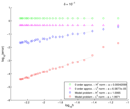
Figure 1: Convergence w.r.t. the mesh size – $\delta=10^{-1}$, $g=1$.

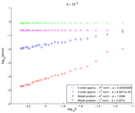
Figure 2: Convergence w.r.t. the mesh size – $\delta=10^{-2}$, $g=1$.

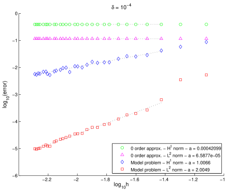
Figure 3: Convergence w.r.t. the mesh size – $\delta=10^{-4}$, $g=1$.

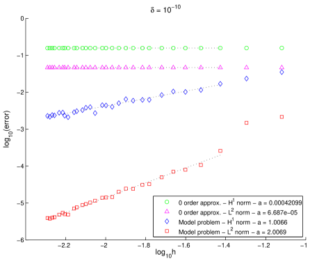
Figure 4: Convergence w.r.t. the mesh size – $\delta=10^{-10}$, $g=1$.

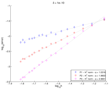
Figure 5: Convergence w.r.t. the mesh size for several orders of approximation – $\delta=10^{-10}$, $g=1$. The cut-off function $\chi$ appearing in the definition of $b_{\log}(\cdot)$ (see (11)) is chosen in $\mathscr{C}^{\infty}(\overline{\Omega})$.

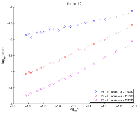
Figure 6: Convergence w.r.t. the mesh size for several orders of approximation – $\delta=10^{-10}$, $g=1$. The cut-off function $\chi$ appearing in the definition of $b_{\log}(\cdot)$ (see (11)) is chosen in $\mathscr{C}^{3}(\overline{\Omega})\setminus\mathscr{C}^{4}(\overline{\Omega})$.

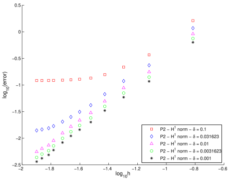
Figure 7: Convergence w.r.t. the mesh size for several values of $\delta$ – $g=1+\sin(\theta)$.

References

[1]
X. Antoine, K. Ramdani, and B. Thierry.
Wide frequency band numerical approaches for multiple scattering
problems by disks.
J. Algorithms Comput. Technol., 6(2):241–259, 2012.
[2]
I. Babuška and M. Suri.
On locking and robustness in the finite element method.
SIAM J. Numer. Anal., 29(5):1261–1293, 1992.
[3]
T. Belytschko and T. Black.
Elastic crack growth in finite elements with minimal remeshing.
Int. J. Numer. Meth. Eng., 45(5):601–620, 1999.
[4]
M.F. Ben Hassen and E. Bonnetier.
Asymptotic formulas for the voltage potential in a composite medium
containing close or touching disks of small diameter.
Multiscale Model. Simul., 4(1):250–277, 2005.
[5]
J.-P. Bérenger.
A multiwire formalism for the FDTD method.
IEEE Trans. Electromagn. Compat.on, 42(3):257–264, 2000.
[6]
V. Bonnaillie-Noël and M. Dambrine.
Interactions between moderately close circular inclusions: the
Dirichlet-Laplace equation in the plane.
Asymptot. Anal., 84(3-4):197–227, 2013.
[7]
V. Bonnaillie-Noël, M. Dambrine, S. Tordeux, and G. Vial.
On moderately close inclusions for the Laplace equation.
C. R. Acad. Sci., Ser. I, 345(11):609–614, 2007.
[8]
V. Bonnaillie-Noël, M. Dambrine, S. Tordeux, and G. Vial.
Interactions between moderately close inclusions for the Laplace
equation.
Math. Models Methods Appl. Sci., 19(10):1853–1882, 2009.
[9]
E. Bonnetier and M. Vogelius.
An elliptic regularity result for a composite medium with
”touching” fibers of circular cross-section.
SIAM J. Math. Anal., 31(3):651–677, 2000.
[10]
M. Bourlard, M. Dauge, M.-S. Lubuma, and S. Nicaise.
Coefficients of the singularities for elliptic boundary value
problems on domains with conical points. III: Finite element methods on
polygonal domains.
SIAM J. Numer. Anal., 29(1):136–155, 1992.
[11]
S.C. Brenner and L.R Scott.
The mathematical theory of finite element methods. 3rd ed.Springer, New York, 2008.
[12]
A. Campbell and S.A. Nazarov.
Une justification de la méthode de raccordement des
développements asymptotiques appliquée à un problème de plaque en
flexion. Estimation de la matrice d’impédance.
J. Math. Pures Appl., 76(1):15–54, 1997.
[13]
M. Cassier and C. Hazard.
Multiple scattering of acoustic waves by small sound-soft obstacles
in two dimensions: mathematical justification of the Foldy-Lax model.
Wave Motion, 50(1):18–28, 2013.
[14]
Z. Chen and X. Yue.
Numerical homogenization of well singularities in the flow transport
through heterogeneous porous media.
Multiscale Model. Simul., 1(2):260–303, 2003.
[15]
P. Ciarlet Jr., B. Jung, S. Kaddouri, S. Labrunie, and J. Zou.
The Fourier singular complement method for the Poisson problem. Part
I: Prismatic domains.
Numer. Math., 101(3):423–450, 2005.
[16]
P. Ciarlet Jr., B. Jung, S. Kaddouri, S. Labrunie, and J. Zou.
The Fourier Singular Complement Method for the Poisson problem. Part
II: axisymmetric domains.
Numer. Math., 102(4):583–610, 2006.
[17]
P. Ciarlet Jr. and S. Labrunie.
Numerical solution of maxwell’s equations in axisymmetric domains
with the fourier singular complement method.
J. Differ. Equ. Appl., 3:113–155, 2011.
[18]
M. Dambrine and G. Vial.
Influence of a boundary perforation on the Dirichlet energy.
Control Cybern., 34(1):117–136, 2005.
[19]
M. Dambrine and G. Vial.
A multiscale correction method for local singular perturbations of
the boundary.
Math. Mod. Num. Anal., 41(01):111–127, 2007.
[20]
J. Dolbow and T. Belytschko.
A finite element method for crack growth without remeshing.
Int. J. Numer. Meth. Eng., 46(1):131–150, 1999.
[21]
C.A. Duarte and J.T. Oden.
An h-p adaptive method using clouds.
Comput. Methods in Appl. Mech. Eng., 139(1):237–262, 1996.
[22]
Y. Efendiev and T.Y. Hou.
Multiscale finite element methods, volume 4 of Surveys and
Tutorials in the Applied Mathematical Sciences.
Springer, New York, 2009.
Theory and applications.
[23]
C. Hazard and S. Lohrengel.
A singular field method for maxwell’s equations: Numerical aspects
for 2d magnetostatics.
SIAM J. Numer. Anal., 40(3):1021–1040, 2002.
[24]
A.M. Il’in.
Study of the asymptotic behavior of the solution of an elliptic
boundary value problem in a domain with a small hole.
Trudy Sem. Petrovsk., (6):57–82, 1981.
[25]
A.M. Il’in.
Matching of asymptotic expansions of solutions of boundary value
problems, volume 102 of Translations of Mathematical Monographs.
AMS, Providence, RI, 1992.
[26]
V.A. Kondratiev.
Boundary-value problems for elliptic equations in domains with
conical or angular points.
Trans. Moscow Math. Soc., 16:227–313, 1967.
[27]
V.A. Kozlov, V.G. Maz’ya, and J. Rossmann.
Elliptic Boundary Value Problems in Domains with Point
Singularities, volume 52 of Mathematical Surveys and Monographs.
AMS, Providence, 1997.
[28]
N. N. Lebedev.
Special functions and their applications.
Dover Publications, Inc., New York, 1972.
[29]
V.G. Maz’ya and S.A. Nazarov.
Asymptotic behavior of energy integrals under small perturbations of
the boundary near corner and conic points.
Trudy Moskov. Mat. Obshch., 50:79–129, 1987.
[30]
V.G. Maz’ya, S.A. Nazarov, and B.A. Plamenevskiĭ.
Asymptotic expansions of eigenvalues of boundary value problems for
the Laplace operator in domains with small openings.
Izv. Akad. Nauk SSSR Ser. Mat., 48(2):347–371, 1984.
[31]
V.G. Maz’ya, S.A. Nazarov, and B.A. Plamenevskiĭ.
Asymptotic theory of elliptic boundary value problems in
singularly perturbed domains, Vol. 1, 2.
Birkhäuser, Basel, 2000.
Translated from the original German 1991 edition.
[32]
J.M. Melenk and I. Babuška.
The partition of unity finite element method: basic theory and
applications.
Comput. Methods in Appl. Mech. Eng., 139(1-4):289–314, 1996.
[33]
S.A. Nazarov.
Asymptotic conditions at a point, selfadjoint extensions of
operators, and the method of matched asymptotic expansions.
In Proceedings of the St. Petersburg Mathematical
Society, Vol. V, volume 193 of Amer. Math. Soc., Transl. Ser. 2,
pages 77–125, Providence, RI, 1999.
[34]
S.A. Nazarov and J. Sokołowski.
Asymptotic analysis of shape functionals.
J. Math. Pures Appl., 82(2):125–196, 2003.
[35]
S.A. Nazarov and J. Sokołowski.
Self-adjoint extensions for the Neumann Laplacian and
applications.
Acta Math. Sin. (Engl. Ser.), 22(3):879–906, 2006.
[36]
D.W. Peaceman.
Interpretation of well-block pressures in numerical reservoir
simulations.
Soc. Pet. Eng. J., 18(3):183–194, 1978.
[37]
C.J. Railton, B.P. Koh, and I.J. Craddock.
The treatment of thin wires in the FDTD method using a weighted
residuals approach.
IEEE Trans. Antennas Propag., 52(11):2941–2949, 2004.
[38]
T. Ransford.
Computation of logarithmic capacity.
Comput. Meth. Funct. Theor., 10(2):555–578, 2011.
[39]
R. Scott.
Optimal estimates for the finite element method on
irregular meshes.
Math. Comp., 30(136):681–697, 1976.