Instability of the finite-difference split-step method on the background of localized solutions of the generalized nonlinear Schrödinger equation

Abstract

We consider numerical instability that can be observed in simulations of localized solutions of the generalized nonlinear Schrödinger equation (NLS) by a split-step method where the linear part of the evolution is solved by a finite-difference discretization. Properties of such an instability cannot be inferred from the von Neumann analysis of the numerical scheme. Rather, their explanation requires tools of stability analysis of nonlinear waves, with numerically unstable modes exhibiting novel features not reported for “real” unstable modes of nonlinear waves. For example, modes that cause numerical instability of a standing soliton of the NLS are supported by the sides of the soliton rather than by its core. Furthermore, we demonstrate that both properties and analyses of the numerical instability may be substantially affected by specific details of the simulated solution; e.g., they are substantially different for standing and moving solitons of the NLS.

Keywords:  Finite-difference methods, Numerical instability, Nonlinear evolution equations.

Short title:  Instability of finite-difference split-step method for NLS

1 Introduction

The split-step method (SSM), also known as the operator-splitting method, is widely used in numerical simulations of evolutionary equations that arise in diverse areas of science: nonlinear waves, including nonlinear optics and Bose–Einstein condensation [1]–[4], atomic physics [5, 6], studies of advection–reaction–diffusion equations [7]–[9], and relativistic quantum mechanics [10]. In this paper we focus on the SSM applied to nonlinear Schrödinger (NLS)-type equations

$$iu_{t}-\beta u_{xx}+G(x,|u|^{2})\,u=0,$$ (1.1)

where $G(x,|u|^{2})$ is some smooth function such that $|G(\infty,|u|^{2})|<\infty$. (This excludes, e.g., the Gross–Pitaevskii equation, where $G(x,|u|^{2})=\alpha x^{2}+\gamma|u|^{2}$.) In fact, we will do most of the analysis for the pure NLS

$$iu_{t}-\beta u_{xx}+\gamma u|u|^{2}=0$$ (1.2)

and will consider differences that occur for the more general equation (1.1), in Sec. 5. Although the real-valued constants $\beta$ and $\gamma$ in (1.2) can be scaled out of the equation, we will keep them in order to distinguish the contributions of the dispersive ($u_{xx}$) and nonlinear ($u|u|^{2}$) terms. Without loss of generality we will consider $\gamma>0$ in (1.2); then solitons exist for $\beta<0$. (For $\gamma<0$, one simply changes the sign of $\beta$ to obtain an equivalent equation.)

The idea of the SSM is that (1.2) can be easily solved analytically when either the dispersive or the nonlinear term is set to zero. This alows one to seek an approximate numerical solution of (1.2) as a sequence of steps which alternatively account for dispersion and nonlinearity:

$$\begin{array}[]{llr}\mbox{for $n$ from $1$ to $n_{\max}$ do:}&&\\ &\bar{u}(x)=u_{n}(x)\,\exp\big{(}i\gamma|u_{n}(x)|^{2}\Delta t\big{)}&\mbox{(nonlinear step)}\vspace{0.2cm}\\ &u_{n+1}(x)=\left\{\begin{array}[]{l}\mbox{solution of \ $iu_{t}=\beta u_{xx}$ at $t=\Delta t$}\\ \mbox{with initial condition $u(x,0)=\bar{u}(x)$}\end{array}\right.&\mbox{(dispersive step)}\end{array}$$ (1.3)

where the implementation of the dispersive step will be discussed below. In (1.3), $\Delta t$ is the time step of the numerical integration and $u_{n}(x)\equiv u(x,n\Delta t)$. Scheme (1.3) can yield a numerical solution of (1.2) whose accuracy is $O(\Delta t)$. Higher-order schemes, yielding more accurate solutions (e.g., with accuracy $O(\Delta t\,^{2})$, $O(\Delta t\,^{4})$, etc.), are known [11, 12, 5], but here we will restrict our attention to the lowest-order scheme (1.3); see also the paragraph after Eq. (3.16) below.

The implementation of the dispersive step in (1.3) depends on the numerical method by which the spatial derivative is computed. In most applications, it is computed by the Fourier spectral method:

$$u_{n+1}(x)={\mathcal{F}}^{-1}\left[\,\exp(i\beta k^{2}\Delta t)\;{\mathcal{F}}[\bar{u}(x)]\;\right]\,.$$ (1.4)

Here ${\mathcal{F}}$ and ${\mathcal{F}}^{-1}$ are the discrete Fourier transform and its inverse, $k$ is the discrete wavenumber:

$$-\pi/\Delta x\leq k\leq\pi/\Delta x,$$ (1.5)

and $\Delta x$ is the mesh size in $x$. However, the spatial derivative in (1.3) can also be computed by a finite-difference (as opposed to spectral) method [13]–[17]. For example, using the central-difference discretization of $u_{xx}$ and the Crank–Nicolson method, the dispersion step yields:

$$i\frac{u_{n+1}^{m}-\bar{u}^{m}}{\Delta t}\,=\,\frac{\beta}{2}\,\left(\frac{u_{n+1}^{m+1}-2u_{n+1}^{m}+u_{n+1}^{m-1}}{\Delta x\,^{2}}+\frac{\bar{u}^{m+1}-2\bar{u}^{m}+\bar{u}^{m-1}}{\Delta x\,^{2}}\right),$$ (1.6)

where $u_{n}^{m}\equiv u(x_{m},n\Delta t)$, $x_{m}$ is a point in the discretized spatial domain:  $-L/2<x_{m}<L/2$, and $L$ is the the length of the domain. Recently, solving the dispersive step of (1.3) by a finite-difference method has found an application in the electronic post-processing of the optical signal in fiber telecommunications [18]. Also, the version of the NLS where the second derivative is replaced by its finite-difference approximation, similarly to the right-hand side (r.h.s.) of (1.6), describes a wide range phenomena from transport of vibrational energy in molecular chains to light propagation in waveguide arrays (see, e.g., [19, 20]).

In what follows we assume periodic boundary conditions:

$$u(-L/2,t)=u(L/2,t);$$ (1.7)

the case of other types of boundary conditions is considered in Appendix A. We will refer to the SSM with spectral (1.4) and finite-difference (1.6) implementations of the dispersive step in (1.3) as s-SSM and fd-SSM, respectively. Our focus in this paper will on the fd-SSM.

Weideman and Herbst [13] used the von Neumann analysis to show that both versions, s- and fd-, of the SSM can become unstable when the background solution of the NLS is a plane wave:

$$u_{\rm pw}=(A/\sqrt{\gamma})\;e^{i\omega_{\rm pw}t},\qquad A={\rm const},\quad\omega_{\rm pw}=|A|^{2}.$$ (1.8)

Specifically, they linearized the SSM equations on the background of (1.8):

$$u_{n}=u_{\rm pw}+\tilde{u}_{n},\qquad|\tilde{u}_{n}|\ll|u_{n}|$$ (1.9)

and sought the numerical error in the form

$$\tilde{u}_{n}=\tilde{A}\,e^{\lambda t_{n}-ikx},\qquad\tilde{A}={\rm const}.$$ (1.10)

The SSM is said to be unstable when for a certain wavenumber $k$ one has:  (i)  Re$(\lambda)>0$ in (1.10), but  (ii)  the corresponding Fourier mode in the original equation (1.2) is linearly stable. Weideman and Herbst found that the s- and fd-SSMs on the background (1.8) become unstable when the step size $\Delta t$ exceeds:

$$\Delta t_{\rm thr,\,s}\approx\Delta x\,^{2}/(\pi|\beta|),\qquad\mbox{for s-SSM \eqref{e_02} \& \eqref{e_03}}$$ (1.11)

and

$$\Delta t_{\rm thr,fd}=\Delta x/\sqrt{2|\beta|\gamma\,|A|^{2}}\quad\underline{\mbox{only for $\beta>0$}},\qquad\mbox{for fd-SSM \eqref{e_02} \& \eqref{e_05}}$$ (1.12)

respectively. Note that for $\beta<0$, the fd-SSM simulating a solution close to the plane wave (1.8) is unconditionally stable. Typical dependences of the instability growth rate, Re$(\lambda)>0$, on the wavenumber is shown in Fig. 1. Let us emphasize that the SSM is unstable for $\Delta t>\Delta t_{\rm thr}$ even though both its constituent steps, (1.3) and either (1.4) or (1.6), are numerically stable for any $\Delta t$.

 

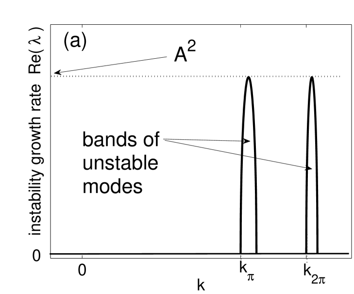
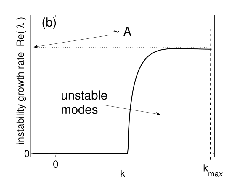
Figure 1: Growth rate of numerical instability of the s-SSM (a) and fd-SSM (b) on the plane-wave background. The dotted horizontal line indicates how the maximum growth rate depends on the wave’s amplitude. In (a), $k_{m\pi}$, $m=1,2,\ldots$ are the wavenumbers where the $m$th resonance condition holds (see [23]): $|\beta|k_{m\pi}^{2}\Delta t=m\pi$.

Solutions of the NLS (and of other evolution equations) that are of practical interest are considerably more complicated than a constant-amplitude solution (1.8). To analyze stability of a numerical method that is being used to simulate a spatially varying solution, one often employs the so-called “principle of frozen coefficients” [21] (see also, e.g., [22, 10]). According to that principle, one assumes some constant value for the solution $u$ and then linearizes the equations of the numerical method to determine the evolution of the numerical error (see (1.9) and (1.10)). However, as we show below, this principle applied to the SSM fails to predict, even qualitatively, important features of the numerical instability (NI).

In this regard we stress — and will subsequently illustrate — that a NI of a particular method applied to a nonlinear equation depends, in general, not only on the method and the equation, but also on the solution which is being simulated. This is similar to the situation with linear stability analysis of particular solutions of a nonlinear equation: some of those solutions may be stable while others may be not. For example, the plane wave (1.8) of the NLS with $\beta<0$ is unstable ([3], Sec. 5.1), while the soliton, given by Eq. (1.13b) below, is stable with respect to small perturbations of their respective initial profiles.

As a step towards understanding NI on the background of a spatially varying solution, we analyzed [23] the instability of the s-SSM on the background of a soliton of the NLS:

$$u_{\rm sol}(x,t)=U_{\rm sol}(x-St)\;\exp\left[i\omega_{\rm sol}t+K_{\rm sol}(x-St)\right];\qquad(\beta<0)$$ (1.13a)

$$U_{\rm sol}(x)=A\sqrt{2/\gamma}\;{\rm sech}\,(Ax/\sqrt{-\beta});\qquad\omega_{\rm sol}=A^{2}+|\beta|K_{\rm sol}^{2},\qquad K_{\rm sol}=S/(2|\beta|).$$ (1.13b)

The parameter $S$, describing the soliton’s speed, was set to 0 in [23]. First, we demonstrated numerically that the instability growth rate in this case is very sensitive to the time step $\Delta t$ and the length $L$ of the spatial domain; also, its dependence on the wavenumber is quite different from that shown in Fig. 1(a). Moreover, the instability on the background of, say, two well-separated (and hence non-interacting) solitons can be completely different from that on the background of one of these solitons. To our knowledge, such features of the NI had not been reported for other numerical methods. In particular, they could not be predicted based on the principle of frozen coefficients. We then demonstrated that all those features could be explained by analyzing an equation satisfied by the numerical error of the s-SSM with large wavenumber $k$:

$$i\tilde{v}_{t}-\omega_{\rm sol}\tilde{v}-\beta(\tilde{v}_{xx}+k^{2}_{\pi}\tilde{v})+\gamma|u_{\rm sol}|^{2}(2\tilde{v}+\tilde{v}^{*})=0,$$ (1.14)

where $\tilde{v}(x,t)$ is proportional to the continuous counterpart of $\tilde{u}_{n}(x)\equiv\tilde{u}(x,n\Delta t)$ defined similarly to (1.9), and $k_{\pi}$ is defined in the caption to Fig. 1. Note that (1.14) is similar, but not equivalent, to the NLS linearized about the soliton:

$$i\tilde{u}_{t}-\omega_{\rm sol}\tilde{u}-\beta\tilde{u}_{xx}+\gamma|u_{\rm sol}|^{2}(2\tilde{u}+\tilde{u}^{*})=0.$$ (1.15)

The extra $k^{2}_{\pi}$-term in (1.14) indicates that the potentially unstable numerical error of the s-SSM has a wavenumber close to $k_{\pi}$.

In this paper we theoretically analyze the NI of the fd- (as opposed to s-) SSM on the soliton background. We will also comment on generic features of NI on more general backgrounds. The NI of the fd-SSM has a number of different features both from the NI of the s-SSM and from the textbook examples of NI of linear equations. Specific features of the NI depend, as we have noted earlier, on both the equation (i.e., (1.1) or (1.2)) and the background solution. They will be listed in respective sections in the text, and most of them will be explained, quantitatively or qualitatively.

Our analysis is based on an equation for the large-$k$ numerical error which, as (1.14), is a modified form of the linearized NLS. However, both that equation and its analysis are substantially different from those [23] for the s-SSM. For example, when the background solution is a standing soliton ($S=0$ in (1.13b)), the modes that render the s- and fd-SSMs unstable are qualitatively different. Namely, for the s-SSM, the numerically unstable modes contain just a few Fourier harmonics and hence are not spatially localized; they resemble plane waves. On the contrary, the modes making the fd-SSM unstable are localized and are supported by the sides (i.e., “tails”) of the soliton. To our knowledge, such “tail-supported” localized modes, as opposed to those supported by the soliton’s core, have not been reported before.

The main part of this manuscript is organized as follows. We begin by studying the instability of the standing soliton, where in (1.13b) $S=0$. In Sec. 2 we present simulation results showing the development of NI of the fd-SSM applied to such a soliton. In Sec. 3 we derive an equation (a counterpart of (1.14)) governing the evolution of the numerical error, and in Sec. 4 obtain its localized solutions that grow exponentially in time. In essence, instead of following a numerical analyst’s approach where one focuses on obtaining a bound for the time step that would guarantee numerical stability, as, e.g., in [16, 24], we employ the procedure used to study (in)stability of nonlinear waves and focus on finding the modes that cause the numerical instability. In doing so, we also find an estimate of the instability threshold as well as the growth rate of those unstable modes. The latter may be useful because, as we will show, in many cases the NI is so weak that it does not affect the simulated solution for a long time. Thus, numerical simulations will produce valid results even if the integration time step exceeds the NI threshold. Using this observation would reduce the computational time.

In Sec. 5 we consider differences in the NI behavior for (a subclass of) the generalized NLS (1.1) compared to that for the pure NLS (1.2). In Sec. 6 we turn to the NI on the background of a moving soliton: $S\neq 0$ in (1.13b). (We assume $S=O(1)$.) As we have pointed out above, one should expect that the NI behavior should depend on the background solution. Indeed, we find that the NIs for the standing and moving solitons are substantially different, both in the required analytical tools and in features. In Sec. 7 we return to the case when the solution of the (generalized) NLS is not moving along $x$. However, unlike in Secs. 2–5, it is oscillating in time. We demonstrate via simulations that in this case, the NI behavior is similar to that for a certain subclass of the generalized NLS, with the background being a stationary, rather than oscillating, soliton. Conclusions of our work, as well as open issues, are summarized in Sec. 8. Appendices A–C pertain to the case of the standing soliton of the pure NLS (1.2). In Appendix A we show how our analysis can be modified for boundary conditions other than periodic. In Appendix B we describe the numerical method used to obtain the localized solutions in Sec. 4. In Appendix C we discuss how the instability analyzed in Secs. 2–4 sets in. Finally, in Appendix D we speculate why the NI reported in Sec. 7 for an oscillating pulse may be similar to that for a standing soliton in a certain potential, reported in Sec. 5.3.

2 Numerics of fd-SSM with standing soliton background

We numerically simulated Eq. (1.2) with $\beta=-1$, $\gamma=2$, and the periodic boundary conditions (1.7) via the fd-SSM algorith (1.3) & (1.6). The initial condition was the soliton (1.13b) with $A=1$ and $S=0$:

$$u_{0}(x)={\rm sech}\,(x)+\xi(x);$$ (2.1)

the noise component $\xi(x)$ with zero mean and the standard deviation $10^{-10}$ was added in order to reveal the unstable Fourier components sooner than if they had developed from a round-off error.

Below we report results for two values of the spatial mesh size $\Delta x=L/N$, where $N$ is the number of grid points:  $\Delta x=40/2^{9}$ and $\Delta x=40/2^{10}$. We verified that, for a fixed $\Delta x$, the results are insensitive to the domain’s length $L$ (unlike they are for the s-SSM [23]) as long as $L$ is sufficiently large. Also, at least within the range of $\Delta x$ values considered, the results depend on $\Delta x$ monotonically (again, unlike for the s-SSM).

First, let us remind the reader that the analysis of [13] on a constant-amplitude background (1.8) for $\beta<0$ predicted that the fd-SSM should be stable for any $\Delta t$. For the soliton initial condition (2.1) and the parameters stated above (with $\Delta x=40/2^{10}$), our simulations showed that the numerical solution becomes unstable for $\Delta t>\Delta x$. For future use we introduce a notation:

$$C=(\Delta t/\Delta x)^{2}\,.$$ (2.2)

In Fig. 2(a) we show the Fourier spectrum of the numerical solution of (1.2), (2.1) obtained by the fd-SSM with $C=1.05$ (i.e., slightly above the instability threshold) at $t=800$. The numerically unstable modes are seen near the edges of the spectral axis. At $t=1000$, these modes are still small enough so as not to cause visible damage to the soliton: see the solid curve in Fig. 2(b). However, at a later time, the soliton begins to drift: see the dashed line in Fig. 2(b), that shows the numerical solution at $t=1100$. Such a drift may persist over a long time: e.g., for $C=1.05$, the soliton still keeps on moving at $t\sim 4000$. However, eventually it gets overcome by noise and loses its identity.

 

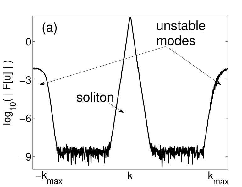
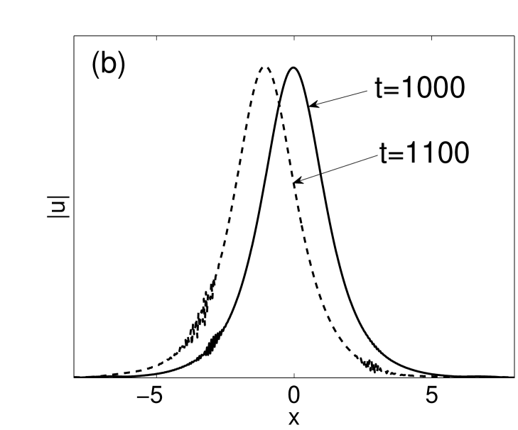
Figure 2: (a)  Fourier spectrum of the unstable numerical solution of (1.2) with initial condition (2.1).  (b)  Effect of numerically unstable modes on the soliton.  Details are presented in the text.

We observed the same scenario for several different values of $\Delta x$, $L$, and $C$ (for $C>1$). The direction of the soliton’s drift appears to be determined by the initial noise; this direction is not affected by the placement of the initial soliton closer to either boundary of the spatial domain. The time when the drift’s onset becomes visible decreases, and the drift’s velocity increases, as $C$ increases.

The soliton’s drift is a nonlinear stage of the development of the numerical instability and will be explained in Sec. 4.2. In the linear stage, the numerically unstable modes are still small enough so that they do not visibly affect the soliton or one another. To describe this stage, we computed a numeric approximation to the instability growth rate  Re$(\lambda)$ defined in (1.10):

$${\rm Re}\,(\lambda)|_{\rm computed}=\frac{\ln\left(\begin{array}[]{c}\max\left|{\mathcal{F}}[u](k)\right|\;\;\mbox{for}\\ \mbox{$k\sim k_{\max}$ at time$=t$}\end{array}\right)-\ln\left(\begin{array}[]{c}\mbox{noise floor}\\ \mbox{at time$=0$}\end{array}\right)}{t},$$ (2.3)

where $k_{\max}=\pi/\Delta x$ (see (1.5)). The so computed values of the instability growth rate are shown in Fig. 3 along with the results of a semi-analytical calculation presented in Sec. 4.1.

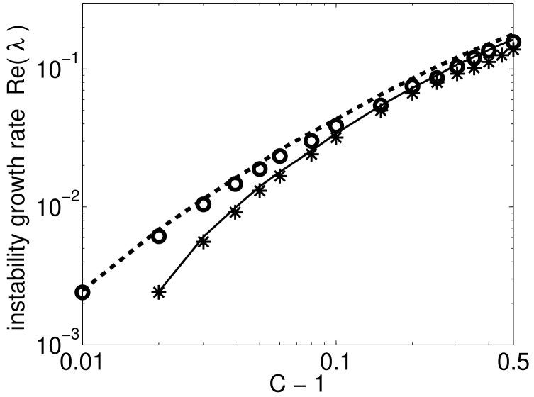
Figure 3: Growth rate of the NI for $\Delta x=40/2^{9}$ (solid line — analysis of Sec. 4, stars — computed by (2.3)) and for $\Delta x=40/2^{10}$ (dashed line — analysis of Sec. 4, circles — computed by (2.3)).

The above numerical results motivate the following three questions:  (i) explain the observed instability threshold $\Delta t$ (see the sentence before (2.2));  (ii) identify the modes responsible for the NI; and  (iii) calculate the instability growth rate (see Fig. 3). In Sec. 4 we will give an approximate analytical answer to question (i). However, answers to questions (ii) and (iii) will be obtained only semi-analytically, i.e., via numerical solution of a certain eigenvalue problem.

3 Derivation of equation for numerical error for fd-SSM

Here we will derive a modified linearized NLS — Eq. (3.15) below — for a small numerical error with a high wavenumber, when the fd-SSM simulates an initial condition close to a standing soliton, (2.1) with $S=0$, of the NLS (1.2). This modified equation will be a counterpart of (1.14), which was obtained for the s-SSM in [23]. The key difference between (1.14) and (3.15) occurs due to the following. In view of periodic boundary conditions (1.7), the finite-difference implementation (1.6) of the dispersive step in (1.3) can be written as

$$u_{n+1}(x)={\mathcal{F}}^{-1}\left[e^{iP(k)}\,{\mathcal{F}}\left[\bar{u}(x)\right]\;\right],$$ (3.1)

$$e^{iP(k)}\equiv\frac{1+2i\beta r\sin^{2}(k\Delta x/2)}{1-2i\beta r\sin^{2}(k\Delta x/2)}=\exp\left[2i\,{\rm arctan}\big{(}2\beta r\sin^{2}(k\Delta x/2)\,\big{)}\right],\qquad r=\frac{\Delta t}{\Delta x\,^{2}},$$ (3.2)

where ${\mathcal{F}}$, ${\mathcal{F}}^{-1}$ were defined after (1.4). For $|k\Delta x|\ll 1$, the exponent in (3.2) equals that in (1.4). However, for $|k\Delta x|>1$, they differ substantially: see Fig. 4. It is this difference that leads to the instabilities of the s- and fd-SSMs being qualitatively different.

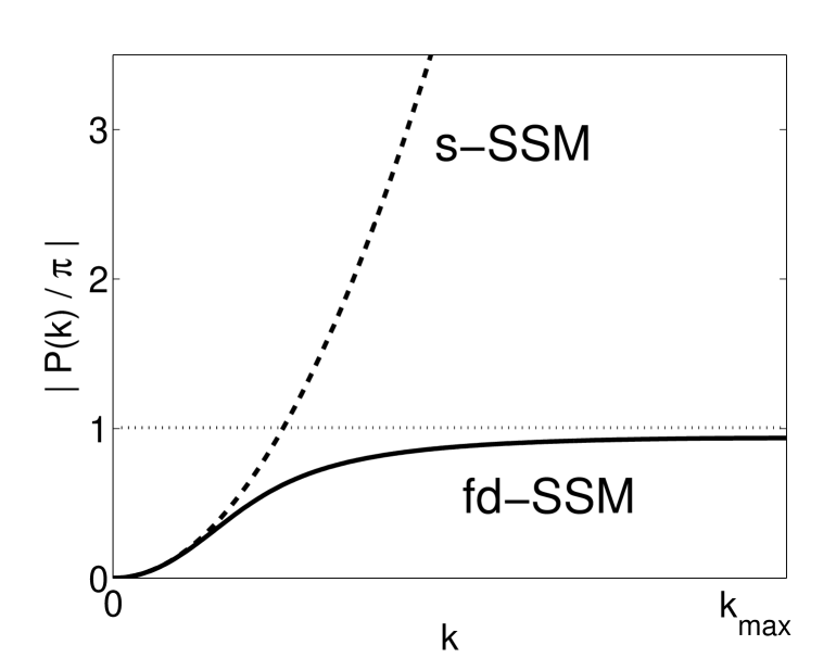
Figure 4: Normalized phase:  $|\beta|k^{2}\Delta t$ for the s-SSM (dashed) and as given by (3.2) for the fd-SSM (solid). In both cases, $r=5$. The horizontal line indicates the condition of the first resonance: $|P(k)|=\pi$.

Using Eqs. (1.3) and (3.1), one can write, similarly to Eq. (3.1) in [23], a linear equation satisfied by a small numerical error $\tilde{u}_{n}$ of the fd-SSM with an arbitrary $k$:

$${\mathcal{F}}\left[\tilde{u}_{n+1}\right]=e^{iP(k)}{\mathcal{F}}\left[e^{i\gamma|u_{\rm b}|^{2}\Delta t}\big{(}\tilde{u}_{n}+i\gamma\Delta t(u_{\rm b}^{2}\tilde{u}_{n}^{*}+|u_{\rm b}|^{2}\tilde{u}_{n})\,\big{)}\;\right]\,.$$ (3.3)

Here $\tilde{u}_{n}$ is defined similarly to (1.9), with $u_{\rm b}$ being either $u_{\rm pw}$ or $u_{\rm sol}$, depending on the background solution. The exponential growth of $\tilde{u}_{n}$ can occur only if there is sufficiently strong coupling between $\tilde{u}_{n}$ and $\tilde{u}_{n}^{*}$ in (3.3). This coupling is the strongest when the temporal rate of change of the relative phase between those two terms is minimized. In [23] we showed that this rate can be small only for those $k$ where the exponent $P(k)$ is close to a multiple of $\pi$. Using (3.2) (see also Fig. 4), we see that this can occur only for sufficiently high $k$ where $\sin^{2}(k\Delta x/2)=O(1)$ rather than $O(\Delta x\,^{2})$. Then:

$$-P(k) = \pi-\frac{1}{|\beta|r\sin^{2}(k\Delta x/2)}+O\left(\frac{1}{r^{3}}\right)$$ (3.4)

$$= \pi-\frac{1}{|\beta|r}-\frac{(k-k_{\max})^{2}\Delta x\,^{2}}{4|\beta|r}+O\left(\frac{1}{r^{3}}+\frac{\big{(}(k-k_{\max})\Delta x\,\big{)}^{4}}{r}\right),$$

where $k_{\max}=\pi/\Delta x$; also recall that $\beta<0$. We have also used that

$$r=\Delta t/\Delta x\,^{2}=C/\Delta t\gg 1,$$ (3.5)

given that the NI was observed in Sec. 2 for $C=O(1)$.

We will now discuss which terms in (3.4) should be retained. First of all, in order to neglect the entire $O$-term, one needs to require that

$$(k-k_{\max})^{2}\Delta x\,^{2}<O(1),$$ (3.6a)

where we have also used (3.5) to neglect the $$O(1/r^{3}) O$$-term. Next, if we keep the third term on the right-hand side (r.h.s.) of (3.4), it should be greater (in the order of magnitude sense) than the discarded -term, whence

$$(k-k_{\max})^{2}\Delta x\,^{2}>O(1/r^{2})=O(\Delta x^{2}).$$ (3.6b)

It is not particularly important where in the range defined by (3.6a) and (3.6b) the value of  $$(k-k_{\max})^{2}\Delta x\,^{2}$$  should be. For example, if we take it in the middle of that range:

$$|k-k_{\max}|=O(1/\sqrt{\Delta x}).$$ (3.6c)

then the three terms on the r.h.s. of (3.4) have orders of magnitude $O(1)$, $O(\Delta x)$, and $O(\Delta x^{2})$. What is important is that we have chosen to keep the third term in (3.4) and hence required (3.6b). We stress that this choice has followed not from our derivation but rather from our numerical results, as illustrated by Fig. 2(a). Indeed, one sees from that figure that the width of the bands of unstable modes, i.e. $|k-k_{\max}|$, is significantly greater than the spectral width of the soliton, which is of order one. In Sec. 6 we will encounter a situation where, in contrast to the above, the third term on the r.h.s. of (3.4) will not need to be kept.

Substituting the first three terms on the r.h.s. of (3.4) into (3.3), using (3.5), and introducing a new variable

$$\tilde{v}_{n}=\left(e^{-i\pi}\right)^{n}\tilde{u}_{n}=(-1)^{n}\tilde{u}_{n},$$ (3.7)

one obtains:

$${\mathcal{F}}[\tilde{v}_{n+1}] = \exp\left(-\frac{i\Delta t}{C\beta}\left\{1+\frac{(k-k_{\max})^{2}\Delta x\,^{2}}{4}\right\}\right)\,\times$$ (3.8)

$${\mathcal{F}}\left[e^{i\gamma|u_{\rm b}|^{2}\Delta t}\,\left\{\tilde{v}_{n}+i\gamma\Delta t(u_{\rm b}^{2}\tilde{v}_{n}^{*}+|u_{\rm b}|^{2}\tilde{v}_{n})\right\}\,\right].$$

Note that (3.8) describes a small change of $\tilde{v}_{n}$ occurring over the step $\Delta t$, because for $\Delta t\rightarrow 0$, the r.h.s. of that equation reduces to ${\mathcal{F}}[\tilde{v}_{n}]$. Therefore we can approximate the difference equation (3.8) by a differential equation, as we will now explain.

First, recall from (3.6a) that the wavenumbers of $\tilde{v}_{n}$ are on the order of $k_{\max}$; hence we seek

$$\tilde{v}_{n}(x)=e^{ik_{\max}x}\,\tilde{w}_{n}(x).$$ (3.9)

The effective wavenumber of $\tilde{w}_{n}$ is then $(k-k_{\max})$, and according to (3.6a) $\tilde{w}_{n}$ varies slowly over the scale $O(\Delta x)$. (One may recognize (3.9) as the standard slowly varying envelope approximation.) Introducing the scaled variables by

$$\chi=x/\epsilon,\quad k_{\rm sc}=(k-k_{\max})\epsilon,\qquad\epsilon=\Delta x/2,$$ (3.10)

one rewrites (3.8) as:

$${\mathcal{F}}_{\rm sc}[\tilde{w}_{n+1}]=\exp\left(-\frac{i\Delta t}{C\beta}\{1+k_{\rm sc}^{2}\}\right)\;{\mathcal{F}}_{\rm sc}\left[e^{i\gamma|u_{\rm b}|^{2}\Delta t}\,\left\{\tilde{w}_{n}+i\gamma\Delta t(u_{\rm b}^{2}\tilde{w}_{n}^{*}+|u_{\rm b}|^{2}\tilde{w}_{n})\right\}\,\right],$$ (3.11)

where now ${\mathcal{F}}_{\rm sc}$ is the Fourier transform with respect to the scaled variables (3.10). In handling the $\tilde{v}_{n}^{*}$ term in (3.8), we have used the fact that on the spatial grid $x_{m}=m\Delta x$, one has:

$$\tilde{v}_{n}^{*}(x_{m})=e^{-ik_{\max}x_{m}}\tilde{w}_{n}^{*}(x_{m})=e^{-i\pi m}\tilde{w}_{n}^{*}(x_{m})=e^{i\pi m}\tilde{w}_{n}^{*}(x_{m})=e^{ik_{\max}x_{m}}\tilde{w}_{n}^{*}(x_{m}).$$

Second, note that the s-SSM (1.3), (1.4) can be written as

$${\mathcal{F}}[u_{n+1}]=e^{i\beta k^{2}\Delta t}\;{\mathcal{F}}\left[e^{i\gamma|u|^{2}\Delta t}\,u\right].$$ (3.12)

When $|\beta|k^{2}\Delta t\ll 1$ and $\gamma|u|^{2}\Delta t\ll 1$, this is equivalent to the NLS (1.2) plus a term proportional to

$$\Delta t\;\left[\beta\partial^{2}_{x},\;\gamma|u|^{2}\right]_{-}u+O(\Delta t\,^{2}),$$ (3.13)

where $[\ldots,\;\ldots]_{-}$ denotes a commutator (see, e.g., Sec. 2.4 in [3]). Equation (3.11) has the form of a linearized Eq. (3.12) with a different coefficient in the dispersion term and with an extra phase. Therefore, (3.11) must be equivalent to a modified linearized NLS, with the modification affecting only the corresponding terms:

$$i\tilde{w}_{t}+(\tilde{w}_{\chi\chi}-\tilde{w})/(C\beta)+\gamma(u_{\rm b}^{2}\tilde{w}^{*}+2|u_{\rm b}|^{2}\tilde{w})=0,$$ (3.14)

plus a term proportional to the linearized form of the commutator (3.13). Neglecting that latter term as small (of order $O(\Delta t)$) compared to the rest of the expression and denoting  $\psi=\tilde{w}\;\exp(-i\omega_{\rm b}t)$, we rewrite (3.14) as:

$$i\psi_{t}+\delta\psi+\psi_{\chi\chi}/(C\beta)+\gamma U_{\rm b}^{2}(\epsilon\chi)\;(2\psi+\psi^{*})=0,$$ (3.15)

where

$$\delta=-\omega_{\rm b}-1/(C\beta).$$ (3.16)

Here $\omega_{\rm b}$ is either $\omega_{\rm pw}$ or $\omega_{\rm sol}$, and $U_{\rm b}$ is either constant or $U_{\rm sol}$, depending on whether the background solution is a plane wave (1.8) or a soliton (1.13b). The modified linearized NLS (3.15) for the fd-SSM is the counterpart of Eq. (1.14) that was derived for the s-SSM.

Our subsequent analysis of the instability of the first-order accurate fd-SSM (1.3) & (1.6) will be based on Eq. (3.15). The instability of the second-order accurate version of this method, where the order of the nonlinear and dispersive steps is alternated in any two consecutive full time steps [11], is the same as that of the first-order version. The instability of higher-order versions (e.g., $O(\Delta t\,^{4})$-accurate) can be studied similarly to how that was done in Ref. [23] for the s-SSM.

The boundary conditions satisfied by $\psi$ are still periodic:

$$\psi(-L/(2\epsilon),\,t)=\psi(L/(2\epsilon),\,t).$$ (3.17)

This follows from the fact that $\tilde{u}_{n}(x)$ satisfies the periodic boundary conditions (1.7) and from (3.9), given that for $k_{\max}=\pi/\Delta x$ and $L/2=M\Delta x$ with some integer $M$,

$$e^{-ik_{\max}L/2}=e^{-iM\pi}=e^{iM\pi}=e^{ik_{\max}L/2}.$$

There are three differences between Eq. (3.15) and the linearized NLS (1.15). Most importantly, (3.15) has the opposite sign of the dispersion term. This is explained by the shape of the curve $P(k)$ for the fd-SSM in Fig. 4 at high wavenumbers, where the curvature is opposite to that at $k\approx 0$. Secondly, unlike the $(-\omega_{\rm sol})$-term in (1.15), the $\delta$-term in (3.15) with $\beta<0$ can be either positive or negative, depending on the value of $C$. Thirdly, the “potential” $U_{\rm b}^{2}(\epsilon\chi)$ (when $U_{\rm b}\equiv U_{\rm sol}$) is a slow function of the scaled variable $\chi$. That is, solutions of (3.15) that vary on the scale $\chi=O(1)$ “see” the soliton as being very wide. This should also be contrasted with the situation for the s-SSM, where the modes described by Eq. (1.14) “see” the soliton as being very narrow [23].

Before proceeding to find unstable modes of Eq. (3.15) with $U_{\rm b}\equiv U_{\rm sol}$, let us note that (3.15) with $U_{\rm b}={\rm const}$ confirms the result of Ref. [13] regarding the instability of the fd-SSM on the plane-wave background. Namely, for $\beta<0$, Eq. (3.15) with $U_{\rm b}={\rm const}$ describes the evolution of a small perturbation to the plane wave in the modulationally stable case (see, e.g., Sec. 5.1 in [3]). That is, for $\beta<0$, there is no NI, in agreement with [13]. On the other hand, for $\beta>0$, Eq. (3.15) describes the evolution of a small perturbation in the modulationally unstable case, and hence the plane wave of the NLS (1.2) can become numerically unstable. The corresponding instability growth rate found from (3.15) and Eq. (5.1.8) of [3] can be shown to agree with the one that can be obtained from Eq. (37) and the next two unnumbered relations in [13]. An example of this growth rate is shown in Fig. 1(b). Also, using our (3.15) and Eq. (5.1.8) of Ref. [3], the threshold value of $\Delta t$ can be shown to be given by (1.12), in agreement with [13].

4 Analysis of numerical instability of standing soliton of NLS

4.1 Unstable modes of modified linearized NLS (3.15)

In this section we focus on the case where the background solution is a soliton with zero velocity ($S=0$ in (1.13b)); hence $\beta<0$ and $U_{\rm b}\equiv U_{\rm sol}(x)$. Substituting into (3.15) and its complex conjugate the standard ansatz [25]  $(\psi(\chi,t),\,\psi^{*}(\chi,t))=(\phi_{1}(\chi),\,\phi_{2}(\chi))\,e^{\lambda t}$  and using yet another rescaling:

$$\begin{array}[]{c}\displaystyle X=\frac{A}{\sqrt{-\beta}}\chi\equiv\frac{2A}{\sqrt{-\beta}}\frac{x}{\Delta x},\qquad D=-\frac{C\beta^{2}}{A^{2}}\delta\equiv\beta^{2}\left(\frac{1}{\beta A^{2}}+C\right),\vspace{0.2cm}\\ \displaystyle\Lambda=\frac{C\beta^{2}}{A^{2}}\lambda,\qquad V(y)=2C\beta^{2}{\rm sech}\,^{2}(y),\end{array}$$ (4.1)

one obtains:

$$\left(\partial_{X}^{2}+D-V(\epsilon X)\left(\begin{array}[]{cc}2&1\\ 1&2\end{array}\right)\,\right)\vec{\phi}\,=\,i\Lambda\sigma_{3}\vec{\phi},$$ (4.2)

where $\sigma_{3}={\rm diag}(1,-1)$ is a Pauli matrix, $\vec{\phi}=(\phi_{1},\,\phi_{2})^{T}$, and $T$ stands for a transpose. If $(\vec{\phi},\,\Lambda)$ is an eigenpair of (4.2), then so are $(\sigma_{1}\vec{\phi},\,-\Lambda)$,  $(\vec{\phi}^{*},\,-\Lambda^{*})$, and $(\sigma_{1}\vec{\phi}^{*},\,\Lambda^{*})$, where

$$\sigma_{1}=\left(\begin{array}[]{cc}0&1\\ 1&0\end{array}\right)$$

is another Pauli matrix. Note also that $\lambda$ is defined in the same way as in (1.10); hence Re$(\Lambda)\neq 0$ indicates an instability. Below we will use shorthand notations $\Lambda_{R}={\rm Re}(\Lambda)$ and $\Lambda_{I}={\rm Im}(\Lambda)$.

We begin analysis of (4.2) with two remarks. First, this equation is qualitatively different from an analogous equation that arises in studies of stability of both bright [25] and dark [26] NLS solitons in that the relative sign of the first and third terms of (4.2) is opposite of that in [25, 26]. This fact is the main reason why the unstable modes supported by (4.2) are qualitatively different from unstable modes of linearized NLS-type equations, as we will see below. While the latter modes are supported by the soliton’s core (see, e.g., Fig. 3 in [27]), the unstable modes of (4.2) are supported by the soliton’s “tails”.

Second, from (4.2) and (4.1) one can easily establish the minimum value of parameter $C$ where an instability (i.e., $\Lambda_{R}\neq 0$) can occur. The matrix operators on both sides of (4.2) are Hermitian; the operator $\sigma_{3}$ on the r.h.s. is not sign definite. Then the eigenvalues $\Lambda$ are guaranteed to be purely imaginary when the operator on the l.h.s. is sign definite [28]; otherwise they may be complex. The third term on the l.h.s. of (4.2) is negative definite, and so is the first term in view of (3.17). The second term, $D$, is negative when

$$C\,<\,1/(|\beta|A^{2}).$$ (4.3)

Thus, (2.2) and (4.3) yield the stability condition of the fd-SSM on the background of a soliton. We will show later that an unstable mode indeed first arises when $C$ just slightly exceeds the r.h.s. of (4.3).

Since the potential term in (4.2) is a slow function of $X$, it may seem natural to employ the Wentzel–Kramers–Brillouin (WKB) method to analyze it. Below we show that, unfortunately, the WKB method fails to yield an analytic form of unstable modes of (4.2). Away from “turning points” (see below) the WKB-type solution of (4.2) is:

$$\vec{\phi}=\left(a_{+}e^{\theta_{+}/\epsilon}+b_{+}e^{-\theta_{+}/\epsilon}\right)\,\vec{\varphi}_{+}+\left(a_{-}e^{\theta_{-}/\epsilon}+b_{-}e^{-\theta_{-}/\epsilon}\right)\,\vec{\varphi}_{-},$$ (4.4)

where $a_{\pm},\,b_{\pm}$ are some constants, and

$$(\theta^{\prime}_{\pm})^{2}=-D+2V\pm\sqrt{V^{2}-\Lambda^{2}},\qquad V\equiv V(\epsilon X),\;\;\theta^{\prime}\equiv d\theta/d(\epsilon X),$$ (4.5a)

$$\vec{\varphi}_{\pm}=\frac{1}{\left[(\theta^{\prime}_{\pm})^{2}(V^{2}-\Lambda^{2})\right]^{1/4}}\,\left(\begin{array}[]{r}\sqrt{\Lambda\pm\sqrt{\Lambda^{2}-V^{2}}}\vspace{0.2cm}\\ -i\sqrt{\Lambda\mp\sqrt{\Lambda^{2}-V^{2}}}\end{array}\right).$$ (4.5b)

At a turning point, say, $X=X_{0}$, the solution (4.4), (4.5b) breaks down, which can occur because the denominator in (4.5b) vanishes. In such a case, one needs to obtain a solution of (4.2) in a transition region around the turning point by expanding the potential:  $V(\epsilon X)=V(\epsilon X_{0})+\epsilon(X-X_{0})\,V^{\prime}(\epsilon X_{0})+\ldots$, and then solving the resulting approximate equation. For a single linear Schrödinger equation, a well-known solution of this type is given by the Airy function. This solution is used to “connect” the so far arbitrary constants $a_{\pm},\,b_{\pm}$ in (4.4) on both sides of the turning point.

Now a turning point of (4.2) is where: either (i) $\theta_{+}^{\prime}=0$ or $\theta_{-}^{\prime}=0$,  or (ii)  $(V(\epsilon X))^{2}-\Lambda^{2}=0$. The former case can be shown (see, e.g., [29]) to reduce to the single Schrödinger equation case, where the solution in the transition region is given by the Airy function. However, at present, no such transitional solution is analytically available in case (ii) [30, 31]. Therefore, the solutions (4.4) canot be “connected” by an analytic formula across such a turning point, and hence one cannot find the eigenpairs ($\vec{\phi}$, $\Lambda$) analytically.

However, the preceding analysis indicates where the unstable modes $\vec{\phi}$ can exist. Based on the past experience with unstable linear modes of nonlinear waves, it is reasonable to assume that unstable solutions of (4.2) must be localized. We now show that localized solutions (4.4) cannot exist around the soliton’s core and thus may only exist at the soliton’s sides. For simplicity, we assume that $\Lambda_{R}\neq 0$ and $\Lambda_{I}=0$ for such a solution, but a more detailed analysis upholds this conclusion for the case $\Lambda_{I}\neq 0$. Note that just above the instability threshold, $D$ is small (see the text before (4.3)), and so is $\Lambda$. On the other hand, near the soliton’s core, $V(\epsilon X)=O(1)$, and hence from (4.5a) one sees that there $\theta_{\pm}^{2}>0$. Thus, both $\theta_{\pm}$ are real, and hence the corresponding (4.4) would grow exponentially away from the soliton’s core. This, however, is not possible because on the scale of Eq. (4.2), the soliton is very wide, and then a mode growing away from its center would become exponentially large before it reaches the turning point. Thus, the only possibility for a localized mode of (4.2) is to be centered at some point at the soliton’s side and decay in both directions away from that point. A straightforward but tedious analysis shows that this is indeed possible when $D>0$ and $\Lambda_{R}\neq 0$.

In Fig. 5 we show the first (i.e., corresponding to the greatest $\Lambda_{R}$) such a mode for $L=40$, $N=2^{9}$ points (hence $\epsilon=\Delta x/2\approx 0.04$), $A=1$, $\beta=-1$, $\gamma=2$. For these parameters, the threshold given by the r.h.s. of (4.3) is $C=1$, and parameter $D$ in (4.2) is related to $C$ by:

$$D=C-1.$$ (4.6)

The numerical method of solving (4.2) is described in Appendix B, and the modes found by this method are shown in Fig. 5(a) for different values of $C$. In Fig. 5(b) we show the same modes obtained from the numerical solution of the NLS (1.2) by the fd-SSM. These modes were extracted from the numerical solution by a high-pass filter, and then the highest-frequency harmonic was factored out as per (3.9). The agreement between Figs. 5(a) and 5(b) is seen to be good. Note that Fig. 5 shows, essentially, the envelope of the unstable mode. The mode not extracted from the numerical solution is shown in Fig. 6(a); it can also be seen at the “tails” of the soliton in Fig. 2(b).

In Fig. 6(b) we show the location of the peak of the first unstable mode, computed both from (4.2) and from the numerical solution of (1.2), versus parameter $C$. The corresponding values of the instability growth rate $\lambda$ were shown earlier in Fig. 3. Let us stress that $\lambda$ for the localized modes of (4.2) was found to be purely real up to the computer’s round-off error ($\sim 10^{-15}$). There also exist unstable modes with complex $\lambda$, but such modes were found to be not localized and to have smaller growth rates than the localized modes.

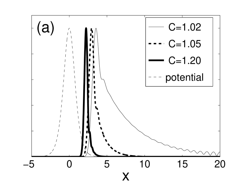
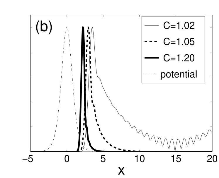
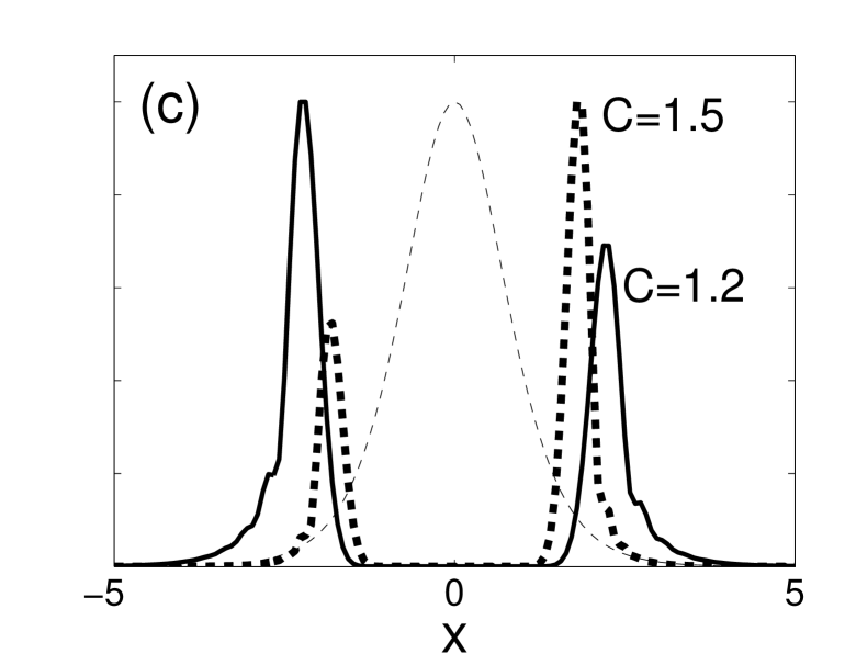
Figure 5: (a)  Profiles of the first localized mode on the right side of the soliton for different values of $C$, as found by the numerical method of Appendix B.  (b)  Same as in (a), but found from the numerical solution of (1.2), as explained in the text.  (c)  The modes at both sides of the soliton found from the numerical solution of (1.2). Note that these modes do not “see” each other because of the barrier created by the soliton, and hence in general have different amplitudes as they develop from independent noise seeds. In all panels, the potential is ${\rm sech}\,^{2}(\epsilon X)$ (see (4.1)) and the amplitude of the mode is normalized to that of the potential.

 

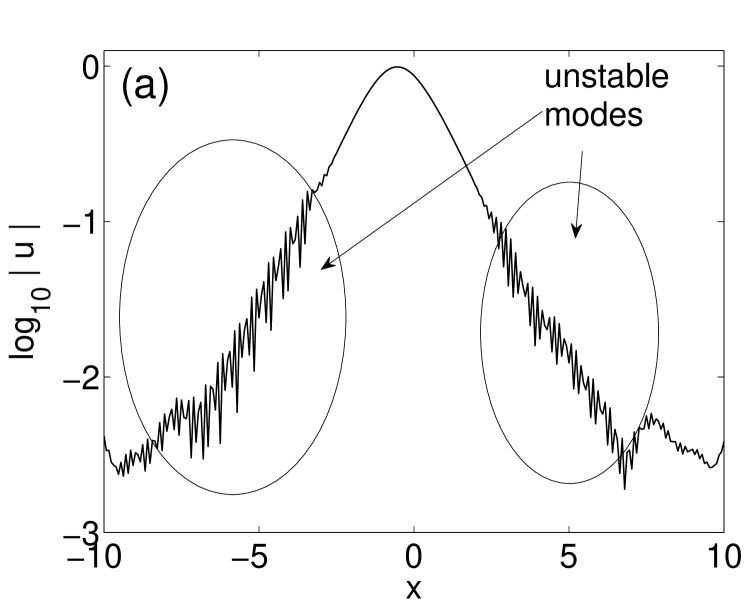
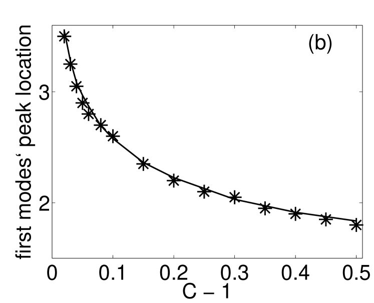
Figure 6: (a)  The numerical solution for $t=1500$ and the same parameters as in Fig. 5, with $C=1.05$.  (b)  Location of the peak of the first localized mode, found by the method of Appendix B (solid line) and from the solution of (1.2) (stars). Similar data for $L=40$ and $N=2^{10}$ are very close and hence are not shown.

   

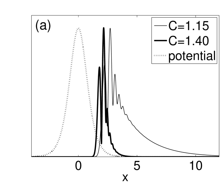
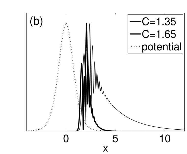
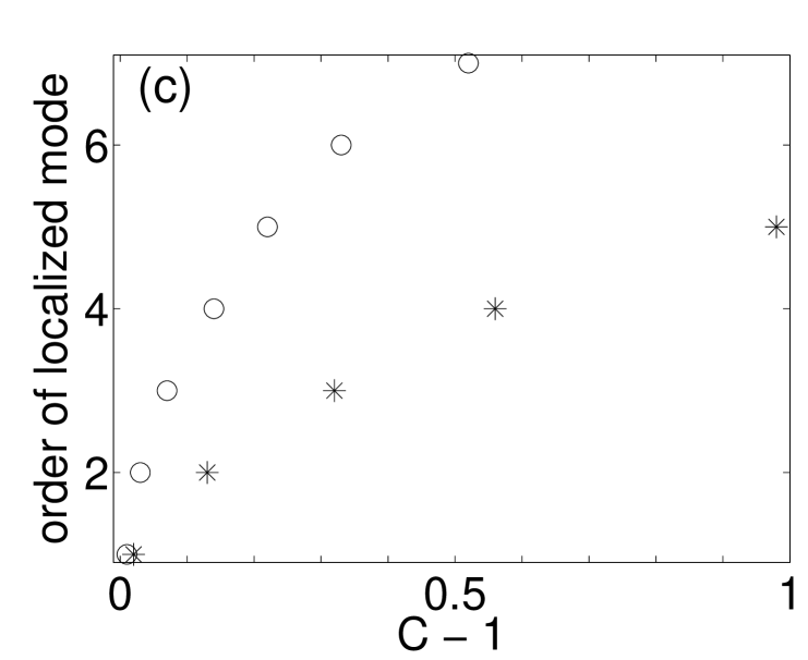
Figure 7: Similar to Fig. 5(a), but for the second (a) and third (b) localized modes.  (c): $C$ values where localized modes of increasing order appear. Stars — for $\epsilon=40/1024$, circles — for $\epsilon=40/2048$.

As $C$ increases from the critical value given by (4.3), the localized unstable mode becomes narrower and also moves toward the center of the soliton. Moreover, higher-order localized modes of (4.2) arise. Typical profiles of the second and third modes are shown in Fig. 7, along with the parameter $C$ for which such modes first become localized within the spatial domain. In Appendix C we demonstrate that the process of “birth” of an eigenmode that eventually (i.e., with the increase of $C$) becomes localized, is rather complicated. In particular, it is difficult to pinpoint the exact value of parameter $C$ where such a mode appears. Therefore, the $C$ values shown in Fig. 7 are accurate only up to the second decimal place.

4.2 Effect of unstable modes on soliton

Let us now show how our results can qualitatively explain the observed dynamics of the numerically unstable soliton — see the text after Eq. (2.2) and Fig. 2(b). Let $\tilde{u}_{\rm unst}$ be the field of the unstable modes at the soliton’s sides. At an early stage of the instabilty, it is much less than the amplitude of the soliton: $|\tilde{u}_{\rm unst}|\ll A$. Also, its characteristic wavenumbers are much greater than those of the soliton: see Fig. 2(a) and (3.6c). Then, to determine its effect on the soliton, one substitutes $u=u_{\rm sol}+u_{\rm unst}$ into the NLS (1.2) and discards all the high-wavenumber terms to obtain:

$$i(u_{\rm sol})_{t}-\beta(u_{\rm sol})_{xx}+\gamma u_{\rm sol}|u_{\rm sol}|^{2}=-2\gamma u_{\rm sol}|u_{\rm unst}|^{2}.$$ (4.7)

This is the equation for a perturbed soliton with the perturbation being, in general, not symmetric about the soliton’s center (see Fig. 5(c)). Indeed, the modes on the left and right sides of the soliton do not “see” each other through the wide barrier created by the soliton’s core and hence can have different amplitudes. Such an asymmetric perturbation is known (see, e.g., [3], Sec. 5.4.1) to cause the soliton to move, which is precisely the effect reported in Fig. 2(b).

5 Numerical instability of soliton in generalized NLS

The analysis of Secs. 3 and 4.1 easily extends to the case when the nonlinearity in (1.1) has a different form than in (1.2) (e.g., is saturable) or when an external potential $\Pi(x)$ is included. Below we focus on the latter situation, i.e. on the subclass of (1.1) described by

$$iu_{t}-\beta u_{xx}+\big{(}\gamma|u|^{2}+\Pi(x)\big{)}u=0.$$ (5.1a)

For brevity, and without loss of generality, we will assume

$$\beta<0.$$ (5.1b)

The opposite choice, i.e. $\beta>0$ (with the corresponding adjustment of signs of both $\gamma$ and $\Pi$), will not affect either real or numerical instabilities of the solution, since Eq. (5.1a) is Hamiltonian.

The soliton solution of (5.1b) has the form similar to (1.13b):

$$u(x,t)=U_{\rm sol}(x)\,\exp[i\omega_{\rm sol}t],$$ (5.2a)

where now $$U_{\rm sol}(x) \omega_{\rm sol}$$ and are found (usually numerically) from the nonlinear eigenvalue problem

$$|\beta|\,(U_{\rm sol})_{xx}+\big{(}\gamma|U_{\rm sol}|^{2}+\Pi(x)\big{)}U_{\rm sol}=\omega_{\rm sol}U_{\rm sol}.$$ (5.2b)

Note that in the presence of potential $\Pi(x)$, the soliton has zero velocity. The evolution equation for the unstable mode, $\psi$, is similar to (3.15):

$$i\psi_{t}+\delta\psi-\psi_{\chi\chi}/(C|\beta|)+\gamma U_{\rm sol}^{2}(\epsilon\chi)\;(2\psi+\psi^{*})+\Pi(\epsilon\chi)\,\psi=0,$$ (5.3a)

where now

$$\delta=-\omega_{\rm sol}+1/(C|\beta|),$$ (5.3b)

with $U_{\rm sol}$ and $\omega_{\rm sol}$ being defined by (5.2b).

Below we will describe three scenarios in which the NI governed by (5.3b) may be qualitatively different from that governed by (3.15) and described earlier in this paper. In the first two scenarios, the differences will be quite obvious, while in the third, it will be less so. Nonetheless, it is this third scenario of the onset of NI that will be shown in Sec. 7 to occur in a yet wider range of situations.

Let us also mention that in all scenarios, the presence of an external potential affects the nonlinear stage of NI (see Sec. 4.2) in a predictable way: due to the confinement by the potential, the soliton would not drift. Rather, it would disintegrate once the numerical noise becomes strong enough.

5.1 External potential with multiple minima

We will show that in this case, unstable modes can be localized only at the absolute minima of the potential. This will result in “stability windows”, i.e. intervals of $C$ values past the NI threshold where NI does not occur.

As an example, we considered Eq. (5.1b) with

$$\beta=-1,\quad\gamma=2,\quad\Pi(x)=1.5\cos^{2}x,\quad\omega_{\rm sol}=1.$$ (5.4)

The numerical parameters were $L=14\pi$ and $N=2^{10}$. The corresponding soliton, found by the numerical method of [32], is shown in Fig. 8. In simulations, the initial condition was taken as that soliton plus small noise, similarly to (2.1). Note that the estimate (4.3) of the threshold value of $C$ beyond which NI may occur is modified as follows (recall (5.1b)):

$$C_{\rm thresh}\,\approx\,\frac{1}{|\beta|\left(\,\omega_{\rm sol}-\min_{x}(\Pi+1\cdot\gamma|U_{\rm sol}|^{2})\,\right)}.$$ (5.5)

The last term in the denominator estimates the “internal” potential, created by the soliton itself. The ‘$1\cdot$’ in front of it indicates that this estimate has used the fact that the smaller eigenvalue of the matrix on the l.h.s. of (4.2) equals 1; see Eq. (11.1a) in Appendix C. Later on we will explain why the expression on the r.h.s. is bound to (slightly) underestimate the threshold value for $C$.

Figure 8: Dashed line: “Internal” potential $\gamma|U_{\rm sol}|^{2}$ ($\gamma=2$), where $U_{\rm sol}$ is the solution of (5.1b) and (5.4). The marked vertical scale pertains to this curve; all other curves are plotted with an arbitrary vertical scale.  Dotted line: External potential $\Pi(x)$.  Solid lines: Absolute value of unstable modes for various values of $C$. (Only one side of each mode is shown; in numerical simulations; one observes such a mode on both sides of the soliton; see Fig. 5(c).)  A: $C\in[1.04,\,1.05]$;  B: $C\in[1.10,\,1.11]$ (this is the second-order mode, similar to that in Fig. 7(a));  C: $C>1.15$.

We have observed no NI until $C=1.04$, at which point the unstable mode appeared as curve A in Fig. 8. Note that the mode is localized near a minimum of $\Pi(x)$. Given that the “internal”’ potential at this $x$ is $2|U_{\rm sol}(x)|^{2}\approx 0.01$, estimate (5.5) yields a smaller NI threshold: $C\approx 1.01$. The discrepancy (i.e., $C=1.01$ versus $C=1.04$) occurs due to neglecting the contribution of $\psi_{\chi\chi}$ in the derivation of estimate (5.5) as explained before (4.3). Since operator $\partial_{\chi\chi}$ is non-positive definite, then accounting for its contribution would decrease the denominator of (5.5) and hence increase $C_{\rm thresh}$. This effect is more conspicuous in the case of the soliton of (5.1b), (5.4) than it was for the NLS soliton in Sec. 4.1 because in the former case, the unstable mode is more localized (compare Fig. 8 and the thin solid curve in Fig. 5(b)), leading to a more negative contribution from $\partial_{\chi\chi}$. From the above discussion and Eq. (5.5), the contribution of operator $\partial_{\chi\chi}$ to the threshold value of $C$ can be roughly estimated as:

$$``\partial_{\chi\chi}"\approx\frac{1}{1.04}-\frac{1}{1.01}\approx-0.03.$$ (5.6)

Let us note, in passing, that the small absolute value of $\partial_{\chi\chi}$ agrees with the fact that while the mode is seen as narrow in $x$-space, it is still very wide in $\chi$-space (recall that $\chi=x/\epsilon$).

In an interval $C\in[1.06,\,1.09]$, NI disappears. This occurs due to the following. As $C$ increases, the unstable mode “wants” to move towards the soliton’s center, similarly to the situation shown in Figs. 6(b). As it moves, the value of $\Pi(x)$ increases and this, according to (5.5), increases the NI threshold, leading to NI’s disappearance.

As $C$ continues to increase, the second-order unstable mode moves from outside the soliton to the location $x\approx 3\pi/2$, where $\Pi(x)\approx 0$, and then NI reappears, being now caused by that second-order mode; see curve B in Fig. 8. With further increase of $C$, that mode moves towards the soliton’s center and away from the minimum of $\Pi(x)$, and NI disappears again.

It reappears when the first-order unstable mode moves into the minimum of $\Pi(x)$ closest to the soliton’s center; see curve C in Fig. 8. In our numerical simulations this was observed starting at $C\approx 1.15$. On the other hand, estimate (5.5) yields $C\approx 1.11$, where we have used that at $x\approx\pi/2$ one has $2|U_{\rm sol}|^{2}\approx 0.1$. However, if we add the contribution of $\partial_{\chi\chi}$ to the denominator of (5.5) and use (5.6), we obtain:  $C\approx 1/(1-0.1-0.3)\approx 1.15$, which is in excellent agreement with the numerical result.

5.2 Bell-shaped potential; $\gamma<0$

We will show that in this case, the unstable mode can appear either at the center or at the “tail” of the soliton.

As an example, we considered Eq. (5.1b) with

$$\beta=-1,\quad\gamma=-1,\quad\Pi(x)=6{\rm sech}\,^{2}x,$$ (5.7)

and used $L=40$ and $N=2^{10}$. Let us note that equations with $\gamma<0$ are not too uncommon; for instance, the generalized NLS with saturable nonlinearity [33] provides an example of a realistic physical system with negative effective nonlinearity.

We will first describe how the soliton of (5.1b), (5.7) depends on $\omega_{\rm sol}$, as this will explain different behaviors of NI observed in this case. By comparing the equation in question with the linear Schrödinger equation with a ${\rm sech}\,^{2}x$ potential, one can see that its soliton exists for $\omega_{\rm sol}\in(0,\,4)$. At $\omega_{\rm sol}=4-0$, it becomes vanishingly small and has the shape of ${\rm sech}\,^{2}x$. As $\omega_{\rm sol}$ decreases, the soliton becomes wider and its amplitude grows, so that at $\omega_{\rm sol}=1$, one has $U_{\rm sol}=2{\rm sech}\,x$. As $\omega_{\rm sol}=+0$, the soliton becomes very wide and its amplitude approaches $\sqrt{6}$. Amplitudes of the soliton at three values of $\omega_{\rm sol}$ are shown in Table 1.

$\omega_{\rm sol}$	$\max{|U_{\rm sol}|}$	$\min\big{(}\Pi-3\gamma|U_{\rm sol}|^{2}\big{)}$	mode’s	$C_{\rm thresh,\;\eqref{e4_308}}$	$C_{\rm thresh,\;numer}$
			location
1	2	$-6$	center	$0.144$	$0.145$
2	$1.657$	$-2.237$	center	$0.237$	$0.241$
3	$1.187$	0	“tail”	$0.334$	see Sec. 5.3

Table 1: NI of the soliton of Eq. (5.1b), (5.7); see text for details. The last two columns list theoretical and numerically observed values for the NI threshold.

The estimate of the the threshold beyond which NI can appear is almost the same as (5.5):

$$C_{\rm thresh}\,\approx\,\frac{1}{|\beta|\left(\,\omega_{\rm sol}-\min_{x}(\Pi-3\cdot|\gamma||U_{\rm sol}|^{2})\,\right)}.$$ (5.8)

Here the ‘$3\cdot$’ in front of the last term occurs because to minimize the expression in parentheses, one needs to use the larger eigenvalue of the matrix on the l.h.s. of (4.2), since now $\gamma<0$. The validity of this estimate is supported by the first two lines of Table 1. We would like to stress three aspects of these results.

First, since for $\omega_{\rm sol}=1$ and 2,  $\min_{x}(\Pi-3\cdot|\gamma||U_{\rm sol}|^{2})$  occurs at $x=0$, the unstable mode appears at the soliton’s center rather than at its “tails”, as was the case in Sec. 4. This mode looks like modes A and C in Fig. 8 except that it is located at $x=0$.

Second, when the unstable mode occurs at the soliton’s center, NI develops very rapidly with respect to parameter $C$. That is, lowering $C$ by 0.001 compared to the value listed in the Table will suppress the NI entirely. On the contrary, at the indicated $C_{\rm thresh}$, magnitude of unstable modes reaches $O(1)$ within $t\sim 100$, which is more than an order of magnitude faster than the unstable modes in Secs. 2 and 4 would do within 1% past $C_{\rm thresh}$.

Third, the case $\omega_{\rm sol}=3$ is different from that of $\omega_{\rm sol}=1$ or 2 in that the unstable mode is predicted by (5.8) to be at the “tails” of the soliton. In that respect, it is similar to the mode discussed in Sec. 4. However, we have also observed substantial differences from the unstable mode of the pure NLS (1.2). These new features of the NI are not specific to having $\gamma<0$, and therefore we report them in a separate subsection, which follows next.

5.3 “Sluggish” numerical instability

We begin by reporting our results for the model (5.1b), (5.7) with $\omega_{\rm sol}=3$. For several values of $C$ near the theoretical threshold $C_{\rm thresh}=1/3$, we ran simulations up to $t=50,000$. Recall that other numerical parameters are $L=40$ and $N=2^{10}$. At $C=0.345$, which is over 3% above the threshold, we have not observed any sign of NI. At $C=0.350$, we have observed an order-of-magnitude growth (from $10^{-8}$ to $10^{-7}$) of high-$k$ harmonics in the Fourier spectrum. In comparison, for the same relative increase above the threshold, $(C-C_{\rm thresh})/C_{\rm thresh}\approx 5$%, the NI growth rate of the pure NLS soliton is about two orders of magnitude greater: see Fig. 3. As we continued to increase $C$, the NI has gradually become stronger; however, this was not monotonic. For example, the evolution of $|{\mathcal{F}}[u](k_{\rm max})|$ at two values of $C$ is shown in Fig. 9(a), where a stronger NI corresponds to the smaller $C$. It is only past $C\approx 0.45$, i.e. 35% above the threshold predicted by (5.8), that the increase of NI’s growth rate with $C$ becomes monotonic.

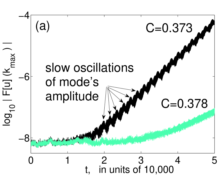
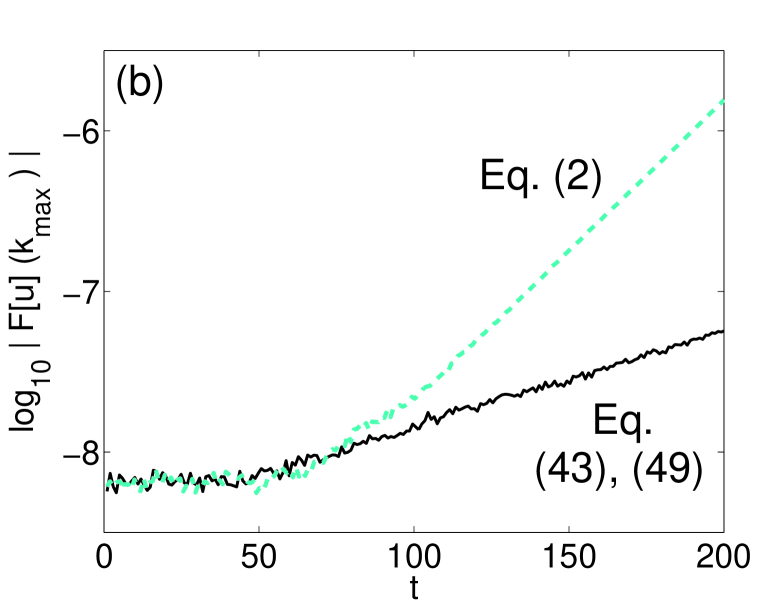
Figure 9: Evolution of the highest Fourier harmonic (see text).  (a)  For Eq. (5.1b), (5.7) with $\omega_{\rm sol}=3$. The lines appear thick because of oscillations on the scale of $t\sim 50$, which is not resolved in this figure. Note also slower oscillations with the period of $t\sim 2000$.  (b)  For Eq. (1.2), $C=1.1$;  for Eq. (5.1b), (5.7), $C=0.45$.

We have called this NI “sluggish” due to its very slow, compared to the pure NLS case, development with the increase of $C$. We have found that it occurs when the external potential $\Pi(x)$ is either wider or significantly taller (or both, as in the case reported above) than the “internal” potential $\gamma|U_{\rm sol}(x)|^{2}$. It is not specific to the particular sign of $\gamma$; for example, it also occurs when in (5.8) one takes $\gamma=+1$ (and, e.g., $\omega_{\rm sol}=5$), as well as for Eq. (5.10) below. We will now list features of this “sluggish” NI and then will provide some insight into them. In Sec. 8 we will speculate on a reason behind the occurrence of “sluggish” NI.

5.3.1 Features of “sluggish” NI

(i)  The unstable mode could remain “hidden” for some time. This is most conspicuous when $C$ is close to the threshold value predicted by (5.8) or, more generally, when the NI is weak. For example, in the cases shown in Fig. 9(a), NI becomes visible only after $t\sim 15,000$ for $C=0.373$ and $t\sim 25,000$ for $C=0.378$.  Motivated by this observation, we revisited our earlier simulations for the soliton of the pure NLS. We have found the same “delayed” NI there as well, except that its starting time was considerably less; see Fig. 9(b).

(ii)  The increase of NI with $C$ is not monotonic; that is, as one increases $C$, NI may sometimes get substantially weaker than it was for a smaller value of $C$. This was illustrated by Fig. 9(a), but has also been observed in many other cases.

(iii)  Growth of unstable modes with time is not monotonic, either. A mild example of it is also shown in Fig. 9(a); in some cases, we even observed oscillations of mode’s amplitude of almost on order of magnitude.

(iv)  The unstable modes of this “sluggish” NI look different from the unstable modes described in Sec. 4. A typical example is shown in Fig. 10. The difference in $x$-space is that while the mode is still almost zero within the soliton (and the external potential), it is not localized outside the soliton. In $k$-space, the latter circumstance is reflected by a peak marked in Fig. 10(a), while the steep decay of the mode towards the soliton’s center is reflected in a broad “plateau”, similarly to what occurred for the unstable mode of the pure-NLS soliton.  Let us note that these characteristics of a “sluggish” unstable mode are generic. Eventually, as $C$ becomes large enough, the shape of the unstable mode becomes qualitatively similar to that described in Sec. 4.

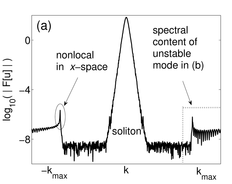
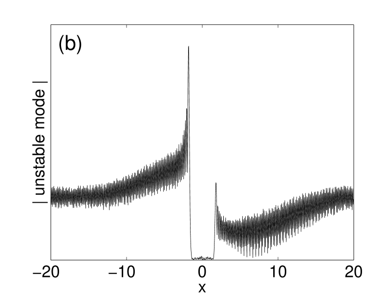
Figure 10: (a) Fourier spectrum of “sluggish” NI; compare to Fig. 2(a).  (b) Absolute value in $x$-space of the unstable mode whose spectral content is shown in the box on the right of panel (a); compare to Fig. 5.

(v)  The fact that the unstable mode may be non-localized in $x$ implies that the growth rate of “sluggish” NI can be affected by the length $L$ of the computational domain, and this was indeed observed in our numerics.

(vi)  Finally, as one decreases $\Delta x$, the relative range  $\Delta C_{\rm rel,\,sluggish}\equiv(C-C_{\rm thresh,\,\eqref{e4_308}})/C_{\rm thresh,\,\eqref{e4_308}}$  where the “sluggish” NI is observed, decreases. For example, if in the simulations reported at the beginning of this subsection one takes $N=2^{11}$ or $N=2^{12}$ (i.e. decreases $\Delta x$ two- and four-fold), then “sluggish” NI turns into “non-sluggish” one around $C=0.42$ and $0.38$, respectively. These values correspond to the $\Delta C_{\rm rel,\,sluggish}<30$% and $\Delta C_{\rm rel,\,sluggish}\approx 15$%, which should be contrasted with $C\approx 0.47$ for $N=2^{10}$, where $\Delta C_{\rm rel,\,sluggish}>40$%.)

5.3.2 Explanation of features of “sluggish” NI

To provide some insight into these features, we have computed eigenvalues and eigenfunctions of the problem

$$\left(\frac{1}{C|\beta|}\partial_{\chi\chi}-\delta-\Pi(\epsilon\chi)-\gamma|U_{\rm sol}(\epsilon\chi)|^{2}\left(\begin{array}[]{cc}2&1\\ 1&2\end{array}\right)\right)\vec{\phi}=i\lambda\sigma_{3}\vec{\phi},$$ (5.9)

obtained from (5.3b). Both the notations and the method of numerical solution of this eigenproblem are the same as for (4.2). Below we report results for the following specific values of parameters:

$$\beta=-1,\quad\gamma=2,\quad\Pi(x)=e^{-0.3x^{2}},\quad\omega_{\rm sol}=1.$$ (5.10)

We have chosen a different $\Pi(x)$ than in (5.7) to emphasize that to bring about a “sluggish” NI it may be sufficient to have the external potential wider, but not necessarily much taller, than the internal one. (Both these potentials corresponding to (5.10) are shown in Fig. 12 below.) However, we have also solved (5.9) for parameters (5.7) and found qualitatively similar results.

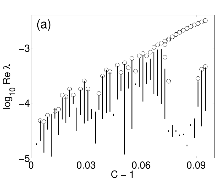
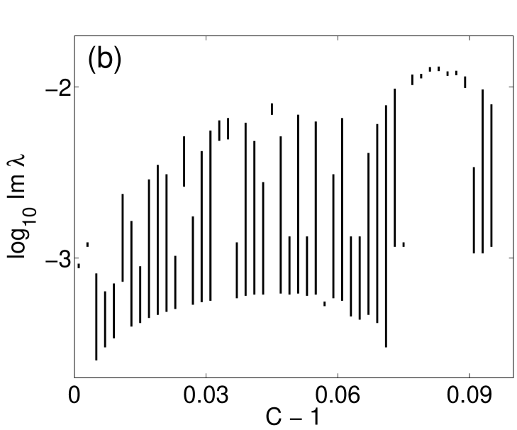
Figure 11: Eigenvalues of (5.9), (5.10) with Re$\,\lambda>0$.  Note that $C_{\rm thresh,\,\eqref{e4_308}}=1$.  (a)  Circles: Purely real eigenvalues.  (a) and (b)  Vertical segments show the intervals of Re$\,\lambda$ and Im$\,\lambda$ corresponding to the smallest $|\lambda|$. (For some $C$, there are also other intervals with larger $|\lambda|$.) It can be seen that around $C=1.077$, two purely real eigenvalues merge into a double eigenvalue, as has observed earlier for the pure NLS case (see Appendix C).

The seemingly mysterious feature (i), i.e. the “delayed” NI, has a simple explanation. The noise $\xi(x)$ in the initial condition (see (2.1)) consists of Fourier harmonics with random phases and random, but similar, amplitudes. The part of each Fourier harmonic that overlaps with the most unstable mode grows, while the rest of the harmonics oscillates or grows at a lower rate. To clarify why this leads to an effective delay in the growth of the Fourier harmonic, we will focus on the case when the unstable mode is nonlocalized, as, e.g., in Fig. 10. In this case, the explanation is most transparent, and it is also then that the “delayed” NI is most conspicuous. The overlap factor between a Fourier harmonic and the most unstable mode,

$${\rm OF}(k)=\left|\int_{-L/2}^{L/2}e^{ikx}u_{\rm mode}dx\right|\,\Big{/}\,\sqrt{L\int_{-L/2}^{L/2}|u_{\rm mode}|^{2}dx},$$ (5.11)

is proportional to the spectrum of the unstable mode; see Fig. 10(a). A point to note is that ${\rm OF}(k)$ has a peak (circled in the figure), i.e. most of the content of the unstable mode is in one Fourier wavenumber, $k_{\rm peak}$. Also, we have verified that

$$\left|{\rm OF}(k_{\rm peak})\right|\sim 0.5.$$ (5.12)

As will become clear shortly, the significance of (5.12) is that this number is substantially less than one. The evolution of the corresponding Fourier harmonic is:

$${\mathcal{F}}[u](k_{\rm peak},t)={\mathcal{F}}[u](k_{\rm peak},0)\left({\rm OF}(k_{\rm peak})\,e^{\lambda_{\rm most}t}+\sum_{j}{\rm OF}(k_{j})e^{\lambda_{j}t}\right),$$ (5.13a)

where $$\lambda_{\rm most} \lambda_{j} \lambda_{\rm most}> \lambda_{j} \lambda_{j}$$ and are the eigenvalues of the most unstable mode and all other modes, respectively; they are shown in Fig. 11. Over long time, the second term on the r.h.s. of (5.13a) is negligible compared to the first one, not only because ReRe but also because of partial cancellation of the summands due to Im all being different. Therefore, asymptotically,

$${\mathcal{F}}[u](k_{\rm peak},t)\approx{\rm OF}(k_{\rm peak})\,{\mathcal{F}}[u](k_{\rm peak},0)e^{\lambda_{\rm most}t}.$$ (5.13b)

Thus, the $k$-peak of the most unstable mode will become visible above the noise floor when  $\left|{\rm OF}(k_{\rm peak})\,e^{\lambda_{\rm most}t}\right|>1$, i.e. for

$$t_{\rm delay}>O(1)/{\rm Re}\lambda_{\rm most},$$ (5.14)

where we have used (5.12). In other words, the weaker the NI, the longer it takes the NI to become observable.

Feature (ii) is immediately explained by Fig. 11(a), which shows that the increase of $\max\,{\rm Re}\,\lambda$ is not monotonic with $C$. This is most notably seen near $C=1.035$, where the NI growth rate drops by almost an order of magnitude.

Feature (iii) is explained by noticing that below $C\approx 1.07$, there are multiple eigenvalues with very similar Re$\,\lambda$. Their eigenmodes grow at very similar rates and interfere, thus causing non-monotonic growth of the numerical error with time.

Feature (iv) is supported by Fig. 12(a). It shows the most unstable mode at $C=1.051$, which is essentially nonlocalized and thus looks qualitatively similar to the mode shown in Fig. 10(b). This should be compared to the localized mode at $C=1.05$ for the pure NLS; see Fig. 5. Even at $C=1.077$, where the two pairs of purely real eigenvalues have almost merged and far exceed real parts of other eigenvalues, the most unstable mode is still not quite localized (Fig. 12(b)).

   

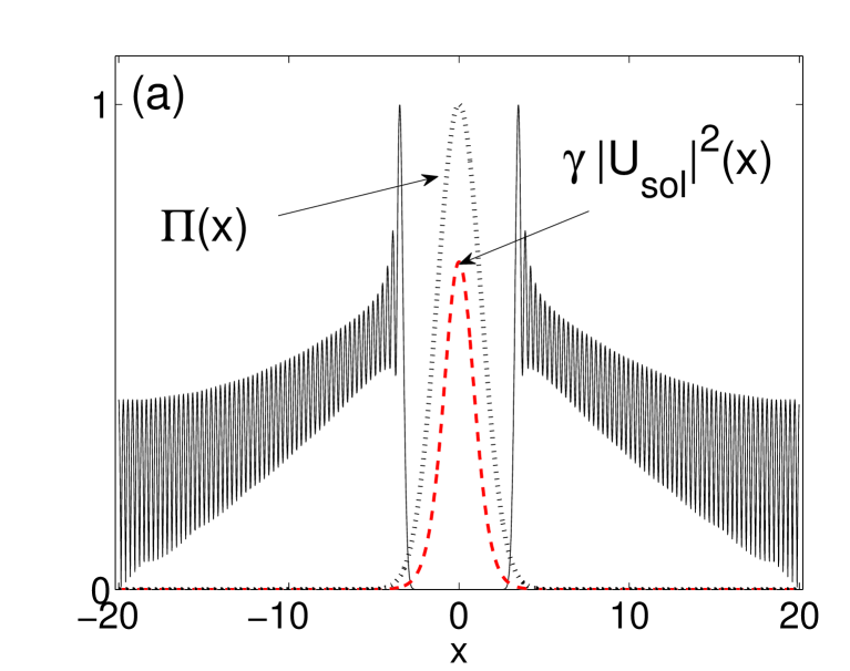
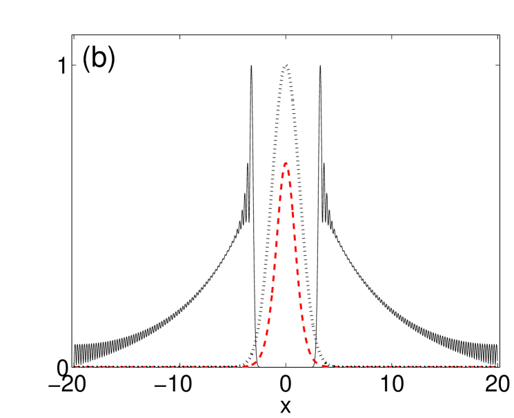
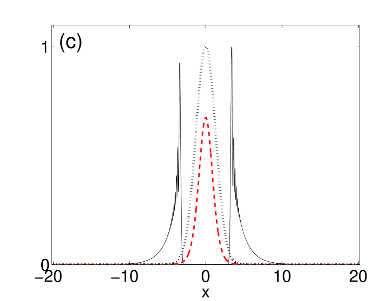
Figure 12: Most unstable mode (solid) and external (dotted) and “internal” (dashed) potentials. The vertical scale pertains to both potentials, while the amplitude of the mode is scaled to one.  (a)  $N=2^{10}$, $C=1.051$;  (b)  $N=2^{10}$, $C=1.077$;  (c)  $N=2^{11}$, $C=1.051$.

Feature (v) is self-explanatory, as has been mentioned earlier. In our numerics we have observed that in its “sluggish” stage, where the most unstable mode is nonlocalized, NI gets, on average, weaker as $L$ increases. However, this dependence is not monotonic. As the most unstable mode becomes essentially localized, the NI’s growth rate, naturally, ceases to depend on $L$.

Feature (vi) is supported by Fig. 12(c), where we show that the most unstable mode becomes localized, and the NI ceases to become “sluggish”, earlier on for smaller $\Delta x$ (or, equivalently, smaller $\epsilon$).

We will encounter “sluggish” NI again in Sec. 7. For now we leave the case of a standing soliton and turn to the moving soliton of the pure NLS (1.2).

6 Numerical instability of moving soliton

The study presented in this section has been motivated by the numerical results of U. Ascher [34], who, to our knowledge, was the first to report the development of NI in the fd-SSM for a moving soliton. More specifically, he considered a collision of two solitons and observed generation of a high-wavenumber ripple for a certain relation between $\Delta t$ and $\Delta x$. However, since a collision is a short-term event, it could not cause NI (which was demonstrated to develop over a very long time: $t\sim 1000$), and hence it is the stationary propagation of an individual soliton that must have lead to the aforementioned NI. Note that due to the periodic boundary conditions, the soliton remained in the computational domain at all times, which justifies the use of the word ‘stationary’ above.

When we learned of Ascher’s results, we have already completed the analysis of NI for a standing soliton and hence initially thought that for a moving soliton, the instability should develop similarly, because the shape of the moving and standing soliton is the same and the only difference is a phase factor: see (1.13b). However, Ascher’s results suggested a qualitatively different scenario of NI. In retrospect, this could be expected given the statement emphasized in the Introduction: NI depends not only on the equation and numerical scheme, but also on the particular solution being simulated. (Let us mention in passing that the NI analysis for a moving plane wave of (1.2) also exhibits some differences from that for a standing plane wave [35].)

We will begin by reporting our own numerical results which demonstrate the same NI as observed by Ascher but for the parameters closer to those used in Secs. 2 and 4. After that we will present an approximate theory of this NI. It will begin as in Sec. 3 but will lead to a different equation to the numerical error than (3.14), which will, therefore, require a qualitatively different analysis. To carry out that analysis, we will have to approximate the soliton by a rectangular box. Such a crude approximation cannot lead to quantitatively accurate predictions about the NI’s threshold, spectral location, and increment. However, it still qualitatively explains a number of observed features of this NI.

6.1 Numerics for the moving soliton, and key observation about spectrum of numerical error

The initial condition in our numerical simulations was taken similarly to (2.1):

$$u_{0}(x)={\rm sech}\,(x)\,e^{iK_{\rm sol}x}+\xi,$$ (6.1)

where $\xi$ is Gaussian noise with amplitude of order $10^{-10}$ and $K_{\rm sol}$ is related to the soliton’s speed as $S=2K_{\rm sol}|\beta|$; see (1.13b). The other parameters: $A=1$, $\beta=-1$, and $\gamma=2$, were as in the previous sections. The Fourier spectrum of a typical numerical solution — for $L=40$, $N=2^{10}$, $C=0.9$, and $t=1500$ — is shown in Fig. 13 for $S=1.89$. (This is an approximation to $S=2$, used so that the exponential factor in (6.1) be exactly periodic in the computational domain.) As the unstable modes continue to grow and become visible on the linear (versus logarithmic) scale on the background of the soliton, in the $x$-space they are observed as high-frequency ripple: see Fig. 7(b) in [34].

Figure 13 illustrates two main differences of the NI for the moving and standing solitons. First, NI for the moving soliton is observed even for $C\,(=(\Delta t/\Delta x)^{2}\,)$ that is less than the threshold value $C=1$ for the standing case (see the text before (4.6)). In fact, we have observed (a weak) NI of the moving soliton with the same parameters even for $C=0.5$; we will comment on it later. Second, the spectrum of each of the numerically unstable modes in Fig. 13(a) (see also Fig. 18(b) below) is considerably narrower than that in Fig. 2(a). We will explain in what follows that this leads to a different equation for the numerical error than (3.14).

 

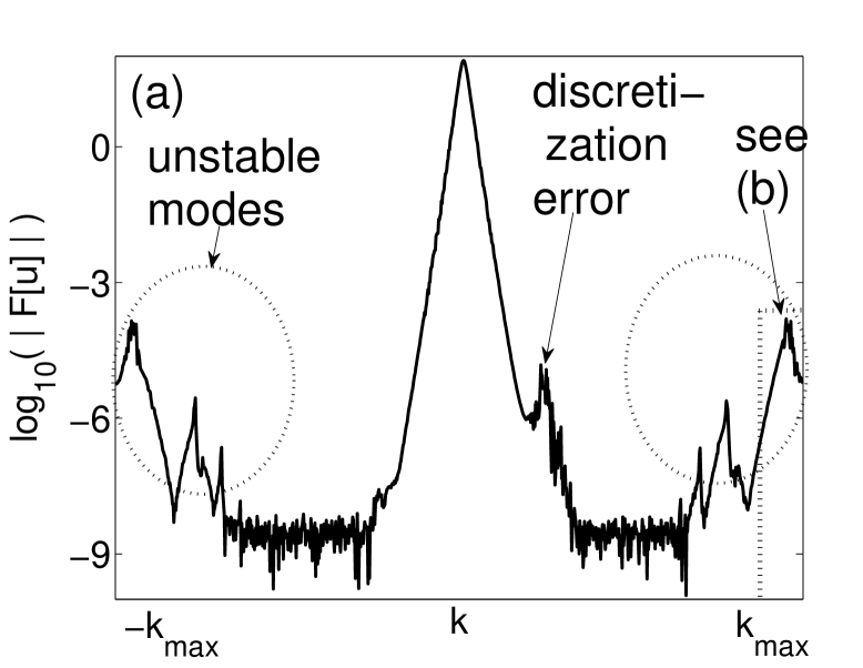
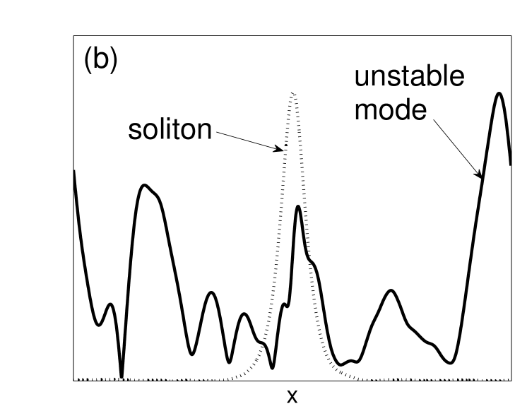
Figure 13: (a) Logarithm of the Fourier spectrum of the numerical solution described in the text. Unstable modes are circled at both ends of the $k$-domain. The discretization error seen on the right of the soliton is due to the approximation of the $u_{xx}$-term in (1.2) by the finite-difference method (1.6).  (b) The unstable mode filtered out by a band-pass filter shown near the right edge of (a). The soliton is shown by the dotted line. Both the soliton and the unstable mode are normalized to have the same amplitude.

Before deriving that equation, let us mention that our derivation will be valid for $S=O(1)$. In the range $0<S<O(1)$, which is intermediate between the case of a standing soliton and the case of a moving soliton considered below, the analysis must be more involved. Indeed, such an analysis should be able to explain a transition between those two cases. However, in the former case, the unstable modes are localized at the sides of the (standing) soliton (see Sec. 4), and such a situation cannot be described even qualitatively using the box approximation for the pulse, which we will (have to) use below for the moving soliton. Thus, the analysis of NI in the intermediate range $0<S<O(1)$ will not be attempted here and remains an open problem.

On the other hand, we note that $K_{\rm sol}=S/(2|\beta|)$ is to be less than approximately $1/\sqrt{|\beta|\Delta t}$ in order for the fd-SSM to yield an accurate solution of the NLS (1.2) [35].

6.2 Modified equation for numerical error on background of moving soliton, and its analysis

The numerical error satisfies Eq. (3.3) for any background solution. From Fig. 13 one can see that the spectrum of unstable modes is approximately symmetric relative to some value $k=O(1)$. It is, therefore, convenient to seek

$$\tilde{u}_{n}=e^{i\omega_{\rm sol}t_{n}+iK_{\rm sol}(x-St_{n})}\left(\tilde{p}_{n}(x)e^{iK_{0}x}+\tilde{q}^{*}_{n}(x)e^{-iK_{0}x}\right),$$ (6.2)

where $(\pm K_{0}+K_{\rm sol})$, with $K_{0}=O(k_{\max})\gg 1$, are the approximate locations of the unstable peaks and $\tilde{p}_{n}(x)$, $\tilde{q}_{n}(x)$ may vary with $x$ on scale $O(1)$. Two notes are in order about the latter assumption. First, it follows solely from numerical results (Fig. 13 and 18(b)), where one sees that the unstable peaks have width of order one in the Fourier space, which implies the above statement about $\tilde{p}_{n}(x)$ and $\tilde{q}_{n}(x)$. Second, the locations of the unstable peaks may differ by an amount of order one from $(\pm K_{0}+K_{\rm sol})$; our analysis will yield approximate expressions both for $K_{0}$ and for those modified locations.

When (6.2) is substituted into (3.3), the next step is to expand the phase $P(k)$. The first step of that expansion is given by the first line of (3.4), but the subsequent expansion is different. Indeed, as discussed in the previous paragraph, the values of $k$ are located within a “distance” of order one of $(\pm K_{0}+K_{\rm sol})$, and therefore also of $\pm K_{0}$ (recall that we have assumed that $S$ and hence $K_{\rm sol}$ are $O(1)$). Therefore, the expansion is:

$$-P(k) = \pi-\frac{1}{|\beta|r\sin^{2}(k\Delta x/2)}+O\left(\frac{1}{r^{3}}\right)$$ (6.3)

$$= \pi-\frac{1}{|\beta|r\sin^{2}(K_{0}\Delta x/2)}+O\left(\frac{1}{r^{2}}\right)\,,$$

where we have also used $\Delta x=O(1/r)$, as in Sec. 3. Then, using Eqs. (3.3), (6.2), (6.3), a transformation  $\{\tilde{p}_{n},\,\tilde{q}_{n}\}=(-1)^{n}\{p_{n},\,q_{n}\}$  (as in (3.7)), the reasoning outlined between Eqs. (3.12) and (3.14), and, finally, the change of variables $(x,t)\longrightarrow(z=x-St,t)$, we obtain:

$$p_{t}-Sp_{z}=i\mu p+i\gamma U_{\rm sol}^{2}(z)\,(2p+q),$$ (6.4a)

$$q_{t}-Sq_{z}=-i\mu q-i\gamma U_{\rm sol}^{2}(z)\,(p+2q),$$ (6.4b)

where $\{p(x,t),\,q(x,t)\}$ are time-continuous counterparts of $\{p_{n}(x),\,q_{n}(x)\}$ and

$$\mu=\frac{1}{C|\beta|\sin^{2}(K_{0}\Delta x/2)}-A^{2}+|\beta|K_{\rm sol}^{2}.$$ (6.5)

The boundary conditions that go with Eqs. (6.4b) are periodic, as in Sec. 3. To be more precise, in light of (6.2) it is  $p(x,t)\exp[i(K_{\rm sol}+K_{0})x]$ and  $q(x,t)\exp[i(K_{\rm sol}-K_{0})x]$ that are to be spatially periodic. However, in all our numerical simulations we have used the initial condition where $K_{\rm sol}$ was on the spectral grid, whence $\exp[iK_{\rm sol}x]$ is periodic. As for the yet unknown $K_{0}$, when later on we determine a range for its values, we will select from that range only the values on the spectral grid; hence $\exp[\pm iK_{0}x]$ will be periodic. Thus, without loss of generality, we require

$$p(-L/2,t)=p(L/2,t),\qquad q(-L/2,t)=q(L/2,t).$$ (6.6)

Since these conditions hold at all times $t$, the first argument of $p$ and $q$ in (6.6) may equally be interpreted as either $x$ or $z$.

Before we use Eqs. (6.4b)–(6.6) to study the NI of a moving soliton, let us note that they, along with (6.2), are the counterparts of the modified linearized NLS (3.15)–(3.17). These two sets of equations are different from one another in two aspects, in addition to the obvious difference of having $S\neq 0$ for the former set. First, Eqs. (6.4b) unlike Eq. (3.15) do not have a second-order spatial derivative. This is a direct consequence of the numerically observed width of the unstable peaks being of order one for the case of moving soliton (Fig. 13), whereas such peaks are considerably wider in the Fourier space for the standing soliton (Fig. 2(a)). This was discussed before Eq. (6.3) and near Eqs. (3.6c), respectively. Second, while coefficient $\delta$ in (3.15) is fixed (for given values of simulated parameters), coefficient $\mu$ in (6.4b) depends on a yet to be determined value $K_{0}$, related to the spectral location of unstable peaks.

Let us now explain why this latter circumstance renders the finding of unstable modes for Eqs. (6.4b), (6.6) more difficult than for (3.15), (3.17). Seeking the solution of (6.4b) in the standard form  $(p(z,t),\,q(z,t))^{T}=\vec{\rho}(z)e^{\lambda t}$, one obtains the following counterpart of (4.2):

$$\left(iS\sigma_{3}\partial_{z}-\mu-\gamma U_{\rm sol}^{2}(z)\left(\begin{array}[]{cc}2&1\\ 1&2\end{array}\right)\,\right)\vec{\rho}=i\lambda\sigma_{3}\vec{\rho},$$ (6.7)

with $\vec{\rho}$ satisfying periodic boundary conditions following from (6.6). Now, when in Sec. 4 we solved the eigenvalue problem (4.2), we selected a value of $C=(\Delta t/dx)^{2}$ and for it found all the unstable modes and their eigenvalues. However, for (6.7) the task is more complicated because $\mu$ depends not only on $C$ but also on $K_{0}$, which not yet known. Then, for a given $C$, one would have to scan through values of $K_{0}$ to determine those special values of $K_{0}$ where one has an unstable mode. Not only would this make the numerical solution in this case considerably more time-consuming, but it would also not provide any insight into why the instability occurs only for some special values of $K_{0}$ but not for all $K_{0}$. Such an insight could only come from an analytical solution of (6.7), but we have been unable to find it for that system of differential equations with a $z$-dependent coefficient $U_{\rm sol}^{2}(z)$ given by (1.13b).

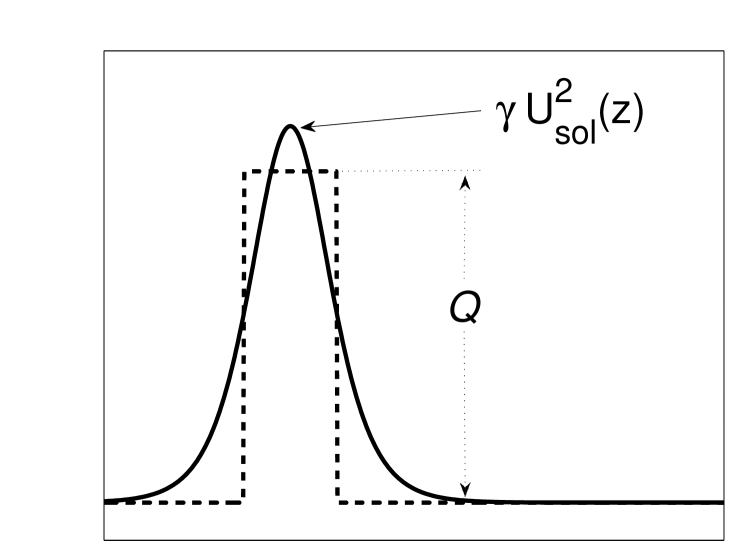
Figure 14: Schematics of a box profile approximating $\gamma U_{\rm sol}^{2}$ in (6.4b).

Therefore, we have resorted to a widely used approximation and replaced $\gamma U_{\rm sol}^{2}(z)$ with a box profile of width $\ell$ and height $Q$, as illustrated in Fig. 14. While such a crude approximation cannot be expected to yield a quantitatively accurate description of NI, it still allows us to understand the nature of unstable modes as well as the dependence of NI’s features on such parameters as $K_{\rm sol}$ (or, equivalently, $S$), the length of the spatial domain $L$, and the mesh size $\Delta x$.

Without loss generality the left-hand edge of the box can be put at $z=0$. Then the solutions of (6.7) with $U_{\rm sol}^{2}$ replaced by the box profile are given by the following expressions inside and outside the box:

$$\begin{array}[]{l}\displaystyle 0\leq z\leq\ell:\vspace{0.2cm}\\ \displaystyle\vec{\rho}=a^{-}_{\rm in}\left(\begin{array}[]{c}\mu+\eta+2Q\\ -Q\end{array}\right)e^{i\kappa^{-}_{\rm in}\,z}+a^{+}_{\rm in}\left(\begin{array}[]{c}-Q\\ \mu+\eta+2Q\end{array}\right)e^{i\kappa^{+}_{\rm in}\,z},\end{array}$$ (6.8a)

$$\begin{array}[]{l}\displaystyle\ell\leq z\leq L:\vspace{0.2cm}\\ \displaystyle\vec{\rho}=a^{-}_{\rm out}\left(\begin{array}[]{c}1\\ 0\end{array}\right)e^{i\kappa^{-}_{\rm out}\,z}+a^{+}_{\rm out}\left(\begin{array}[]{c}0\\ 1\end{array}\right)e^{i\kappa^{+}_{\rm out}\,z},\end{array}$$ (6.8b)

where

$$\eta=\sqrt{(\mu+2Q)^{2}-Q^{2}},\qquad\kappa^{\pm}_{\rm in}=(-i\lambda\pm\eta)/S,\qquad\kappa^{\pm}_{\rm out}=(-i\lambda\pm\mu)/S.$$ (6.9)

The constants $a^{\pm}_{\rm in,\,out}$ are found using the continuity of this solution at $z=\ell-0$ and $z=\ell+0$ and at $z=L$ and $z=0$, with the latter condition being equivalent to the periodic boundary condition. The existence of nontrivial solutions of the resulting linear system determines the eigenvalue $\lambda$:

$$e^{\lambda L/S}=R\pm\sqrt{R^{2}-1},$$ (6.10a)

$$R=\cos\Phi_{+}+\frac{Q^{2}}{(\mu+\eta+2Q)^{2}-Q^{2}}\left(\cos\Phi_{+}-\cos\Phi_{-}\right).\vspace{0.2cm}$$ (6.10b)

$$\Phi_{\pm}=(\mu(L-\ell)\pm\eta\ell)/S$$ (6.10c)

Eigenvalues with  Re$\lambda>0$ exist for

$$|R|>1.$$ (6.11)

Thus, (6.11) along with (6.10cb,c) is the condition of NI of a moving soliton.

6.3 Features of numerical instability of moving soliton and their explanation

As we announced in the Introduction, the focus of our study is to understand what modes cause NI and, if possible, estimate their growth rate and a threshold for their appearance. Numerical results of Sec. 6.1 presented evidence, and the analysis of Sec. 6.2 confirmed, that these unstable modes are delocalized, plane-wave-like packets. The NI is caused by a pair of these waves, denoted as $p$ and $q$ in Sec. 6.2, repeatedly (due to the periodic boundary conditions) passing through the soliton and interacting with each other. This situation should be contrasted with the unstable modes of standing solitons considered in Secs. 2–5.2, which are localized and “pinned” at the “tails” of its host pulse.

Below we will show how to use Eqs. (6.10c), (6.11) to explain qualitatively, and sometimes even quantitatively, a number of features (including the growth rate) of the NI of a moving soliton, observed in numerical simulations.

• The height and spectral width of unstable peaks decrease as their wavenumber $|k|$ decreases;

• The wavenumbers of the unstable peaks vary in inverse proportion to $\Delta x$;

• The wavenumbers of the peaks are not symmetric about $K_{\rm sol}$, as one could have concluded from (6.2);

• The instability growth rate, Re$\lambda$, varies in inverse proportion to the length $L$ of the computational domain;

• The instability decreases as $C$ is decreased or $K_{\rm sol}$ is increased.

Feature (i) is illustrated by Fig. 14(a), while details on the other features will be given as we proceed.

A convenient way to analyze the NI condition is to consider a parametric representation $R=R(\mu)$ and $K_{0}=K_{0}(\mu)$, where for the latter one inverts (6.5):

$$K_{0}=\frac{2}{\Delta x}{\rm arcsin}\sqrt{\frac{1}{C|\beta|(\mu-|\beta|K_{\rm sol}^{2}+A^{2})}}.$$ (6.12)

The resulting plot of $|R|$ versus $K_{0}$ is shown in Fig. 15(a) for the same parameters as used for Fig. 13. For other parameters, the plot $R=R(K_{0})$ looks qualitatively similar. We have also used the values

$$\ell=1.76,\qquad Q=4/\ell,$$ (6.13)

where the first is the full width at half maximum of the ${\rm sech}\,^{2}$ profile and the second follows from $Q\ell=\int_{-\infty}^{\infty}\gamma U_{\rm sol}^{2}(z)dz=4$ for $A=|\beta|=1$. In Fig. 15(b) we show a detailed view of (a) that demonstrates that the NI condition (6.11) is satisfied only in narrow bands of wavenumbers $k$. As we noted before (6.6), values of $K_{0}$ must be on the spectral grid, and hence the increasingly narrow bands where $|R|>1$ occurring towards the decreasing values of $K_{0}$ may simply miss points on the spectral grid. This, along with the fact that the “tips” of $|R|$ that exceed 1 become smaller as $K_{0}$ decreases explains feature (i) stated above.

 

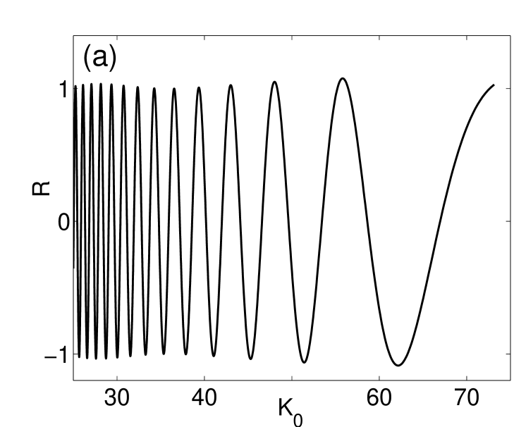
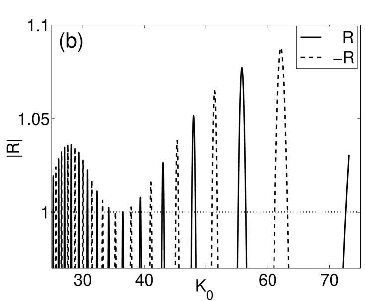
Figure 15: (a) $R(K_{0})$  and (b) a detailed view of (a) near $\pm R(K_{0})=1$.

Feature (ii) is illustrated by Table 2. The simulation parameters are the same as those used for Fig. 13, except that we have varied $C$ and also compared the cases of $N=2^{10}$ and $N=2^{11}$ grid points, so that the corresponding $\Delta x$ differ by a factor of 2. The locations of the respective peaks of unstable modes is seen to differ by an approximately reciprocal factor. An explanation for this follows directly from (6.12).

$C$	$k^{\pm}_{\rm peak},\;N=2^{10}$			$k^{\pm}_{\rm peak},\;N=2^{11}$
0.9	$77.0$	$62.5$	$56.2$	$154.4$	$125.0$	$112.2$
	$-76.2$	$-61.8$	$-55.6$	$-153.3$	$-124.4$	$-111.7$
1.0	$63.9$	$56.4$	$51.5$	$128.0$	$112.6$	$102.9$
	$-63.1$	$-55.7$	$-50.9$	$-127.2$	$-112.0$	$-102.4$
1.25	$71.8$	$58.7$	$52.0$	$144.5$	$117.2$	$103.8$
	$-70.7$	$-57.8$	$-51.2$	$-143.4$	$-116.2$	$-103.0$
1.50	$74.0$	$57.6$	$50.5$	$149.5$	$115.3$	$100.7$
	$-72.8$	$-56.6$	$-49.5$	$-147.7$	$-114.2$	$-99.7$

Table 2: Wavenumbers of the three most unstable peaks; $k^{+}>0,\,k^{-}<0$. For $C\geq 1$ the outer peaks (those with larger $|k_{\rm peak}^{\pm}|$) contain several grid points; only the wavenumber of the maximum $|{\mathcal{F}}[u](k)|$ is listed in those cases.

Results of Table 2 also illustrate feature (iii): the positive and their respective negative peaks are not symmetric about $K_{\rm sol}$. That is,

$$(k^{+}_{\rm peak}+k^{-}_{\rm peak})/2\neq K_{\rm sol}.$$ (6.14)

The l.h.s. of this formula is plotted in Fig. 16(a). The analytical estimate for this quantity is obtained as follows. Since at any given time the soliton occupies only a small part of the computational domain, the unstable mode is described for the most part by its “outside of the box” expression (6.8b). Along with the expression (6.9) for $\kappa^{\pm}_{\rm out}$ and the fact that for the unstable modes $\lambda$ is purely real (see (6.10a) and (6.11)) this implies that $\{p,\,q^{*}\}\propto\exp[-i(\mu/S)z]$. Then from (6.2) it follows that

$$k^{\pm}_{\rm peak}=\pm K_{0}+K_{\rm sol}-\mu/S,$$ (6.15)

which confirms (6.14).

 

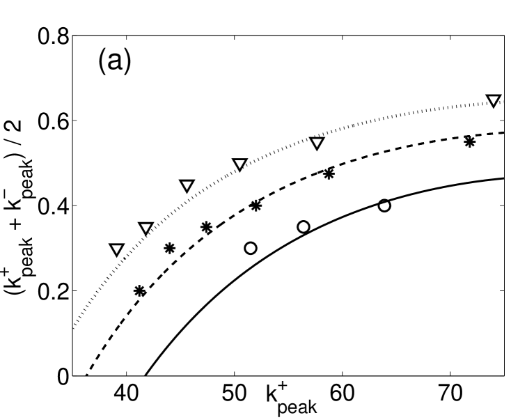
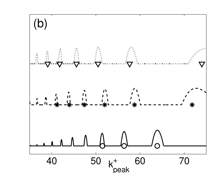
Figure 16: (a) The l.h.s. of (6.14) versus the wavenumber of unstable peaks with $k>0$. Solid, dashed, and dotted lines are the analytical expressions obtained from (6.15) for $C=1,\,1.25,\,1.5$ and the parameters stated in the text. Circles, stars, and triangles are the respective numerical values.  (b) Line and symbol styles pertain to the same cases as in (a). Lines are obtained from the analytical expressions for  $\max(|R|,\,1)$, so that the “bumps” indicate locations of bands of unstable modes. Symbols indicate the locations of numerically obtained unstable peaks. The data for different values of $C$ are vertically shifted for clarity.

Figure 16 demonstrates that the locations of unstable peaks are quite accurately predicted by our approximate analysis. However, this analysis considerably (by a factor of order two for $C\approx 1$) overestimates the instability growth rate. Moreover, as $C$ decreases, the discrepancy between the analytical and numerically observed growth rates increases.

Yet, our analysis easily explains feature (iv), whereby the instability growth rate scales in inverse proportion to the length of the computational domain (assuming that it far exceeds the width of the soliton). To that end, we will first explain why one typically has

$$|R|-1\ll 1\qquad\mbox{where $|R|>1$},$$ (6.16)

as seen in Fig. 15. For $C$, $A$, $K_{\rm sol}$ all of order one, $\mu$ is also of order one; see (6.5). (For the specific values $A=K_{\rm sol}=|\beta|=1$ used here, $\mu\geq 1/C$.) Then, even if we conservatively assume $\mu>0$, then from (6.9) one has $\eta/Q>\sqrt{3}$, and then

$$(\mu+\eta+2Q)^{2}/Q^{2}>(\sqrt{3}+2)^{2}\approx 14.$$ (6.17)

We stress that this is a conservatively low estimate; in our simulations the respective values were higher than about 22. Relation (6.17) implies that the second term in (6.10b) is small. From this one concludes that the “bumps” of $|R|$ occur where $\Phi^{+}\approx\pi n$ for some integer $n$ and that

$$|R|-1\leq 2/\left(\big{(}(\mu+\eta)/Q+2\big{)}^{2}-1\right),$$ (6.18a)

which in view of (6.17) and the note below it we regard as as small number. Combining this with (6.10a) one obtains

$$\lambda\approx\sqrt{2}(S/L)\sqrt{|R|-1},$$ (6.18b)

which provides the reason behind feature (iv).

Formulas (6.18b) and (6.5) also explain why increasing $K_{\rm sol}$ (and hence $S=2|\beta|K_{\rm sol}$) eventually suppresses the NI, which was stated as part of feature (v). Below we will present our argument as a crude estimate but will confirm it with analytical expressions following from our analysis above and also by results of numerical simulations. For the purpose of this estimate we will assume that the first two terms on the r.h.s. of (6.5) approximately cancel each other, and then $\mu\sim K_{\rm sol}^{2}$. With the same accuracy, from (6.9) we have $\eta\sim K_{\rm sol}^{2}+2Q$, and then from (6.18b) we find

$$\max\,\lambda\propto K_{\rm sol}/(K_{\rm sol}^{2}/Q+2).$$ (6.19)

This shows that as $K_{\rm sol}$ increases, the instability growth rate eventually vanishes, although it does grow initially as $K_{\rm sol}$ increases from zero. These conclusions are qualitatively confirmed by Fig. 17. As an aside, let us note that the broad “pedestals” of the unstable peaks for $K_{\rm sol}=0.3$ and $0.5$ seen in Fig. 17(b) are reminiscent of the spectrally broad unstable mode of a standing soliton in Fig. 2(a). This agrees with our remark, made before (6.2), that for sufficiently small $K_{\rm sol}$ (or $S$) there should be a regime where the NI of a moving soliton turns into that of a standing soliton; as we have stated earlier, our analysis does not capture this regime.

 

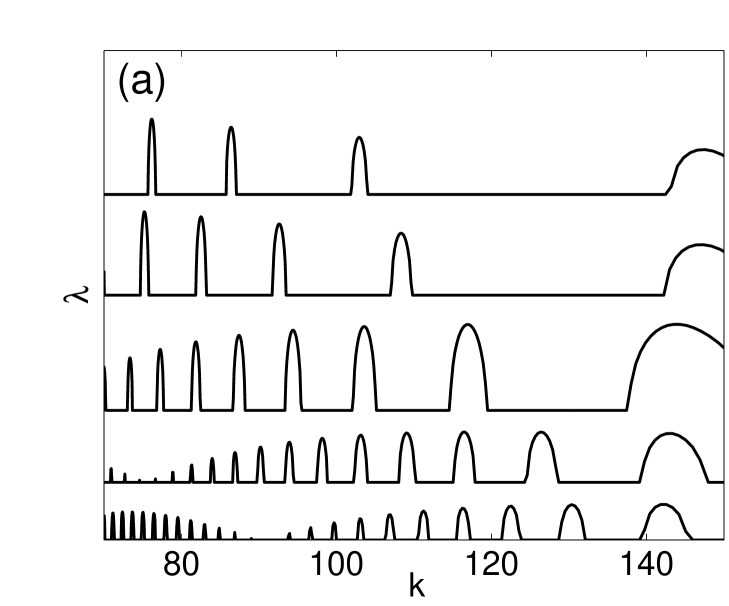
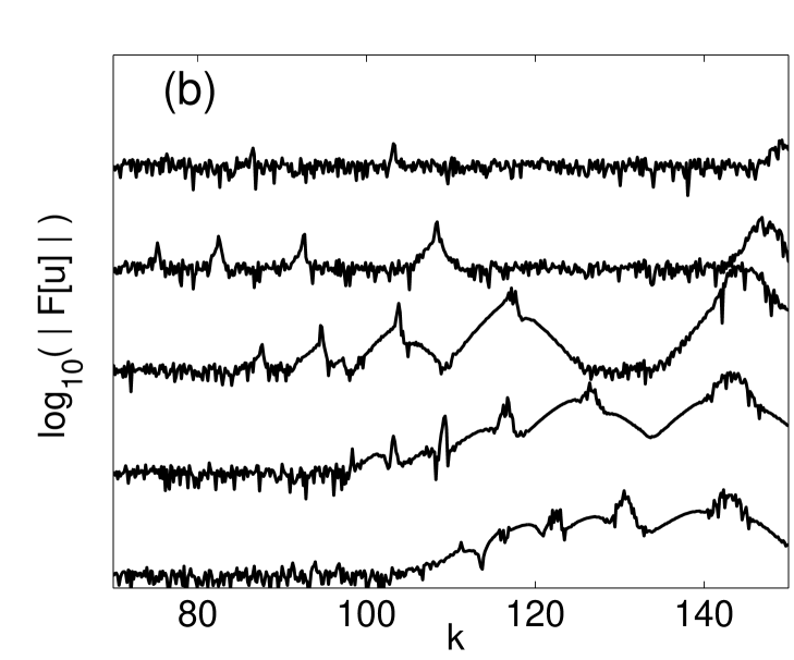
Figure 17: (a) NI growth rate, computed from (6.18b), as a function of wavenumber. The parameters are as previously described in the text, except that $C=1.25$, $K_{\rm sol}$ is varied as stated below, and $N=2^{11}$. (This larger $N$, leading to a smaller $\Delta x$, is needed to keep the discretization error due to the finite-difference approximation (1.6) sufficiently small for the larger values of $K_{\rm sol}$.) The curves, from bottom to top, correspond to $K_{\rm sol}=0.31,\,0.47,\,0.94,\,1.57,\,2.04$. Note that only the higher-$k$ part of the spectrum is shown.  (b) The results of numerical simulations for the same respective parameters as in (a).

The other part of feature (v) — that as $C$ decreases, the NI growth rate decreases — is explained similarly to the above. Indeed, it follows from (6.5) that $\mu$ increases as $C$ decreases, which via (6.18b) implies that $\lambda$ decreases. The main difference from (6.19) here is that this decrease occurs monotonically with $C$.

To conclude this section, let us note that the “delayed” NI, first reported in Sec. 5.3, is also observed for the moving soliton. Because of estimate (5.14), this phenomenon is most noticeable for lower values of $C$. For example, for $C=0.7$, NI may become visible around $t=1300$, as shown in Fig. 18(a). The delay time could be varied by varying the seed of the random number generator for the background noise in the initial condition (6.1). This is illustrated in Fig. 18(a) and is in agreement with the explanation of the “delayed” NI given in Sec. 5.3.

 

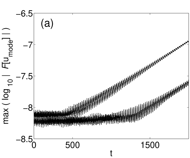
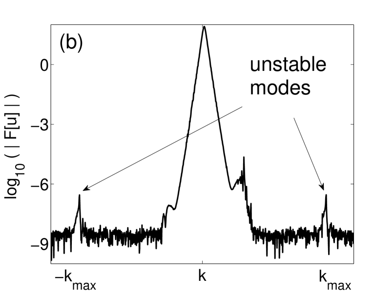
Figure 18: (a) Evolution of the right peak of the unstable mode for two different noise realizations in initial condition (6.1).  (b) Fourier spectrum of the numerical solution corresponding to the smaller delay time in (a); simulation parameters are the same as in Fig. 13, except that $C=0.7$ and $t=2000$.

7 Numerical instability of oscillating solutions of Eq. (5.1b)

In the the previous sections we have analyzed the NI on the background of solitons of the pure and generalized NLS which have stationary shape. Here we will extend those studies to the NI of solutions whose shape varies in time. As before, we will be concerned with the NI that is weak, i.e. takes a long time to develop. When the background solution’s shape is changing, the development of weak NI is possible only when those changes are repetitive. Otherwise, the factors leading to NI will not be able to accumulate coherently, and hence NI would not be able to occur. Therefore, solutions where weak NI could occur must be periodic or near-periodic in time. Below we will restrict our attention to such solutions whose center is not moving; i.e., they extend the standing solitons considered in Secs. 4 and 5. We will show that NI on the background of such oscillating pulses is similar to the “sluggish” NI reported in Sec. 5.3.

In all simulations reported below, we used $\beta=-1$ and $\gamma=2$.

7.1 “Sluggish” numerical instability of oscillating pulses

We began by simulating the NLS (1.2) with the initial condition and length of the computational domain given by:

$$u_{0}(x)={\rm sech}\,(x)\cdot e^{-(x/3)^{4}}+0.2\cos(2\pi x/L)+\xi(x),\qquad L=20,$$ (7.1)

instead of (2.1). Here the exponential factor was used to ensure zero (to numerical accuracy), and hence periodic, boundary conditions at this shorter $L$ than in the previous sections. Near $x=0$, the solution resembles a soliton, whose amplitude and width oscillate in time; the “pedestal” outside the pulse oscillates as well. By varying $C$ around 0.25 (see below), we observed the “sluggish” NI with all its features described in Sec. 5.3.3. The most notable feature is still (i): the NI may take a long time to develop; recall Figs. 8 and 18(a). For example, for $N=2^{9}$ and $C=0.226$, it takes $t>10,000$ for the NI to become distinguishable above the noise floor; by $t=50,000$ it grows only by half an order of magnitude. At $C=0.265$, it rises from the noise floor around $t\sim 6,000$ and grows by an order of magnitude by $t=20,000$.

We have considered possible reasons that could cause “sluggish” NI in this case. From Secs. 4 and 5 we have recalled that the unstable mode was found at the “tails” of the pulse. Since the “tails” are being constantly affected by the oscillating “pedestal”, could that quasi-periodic motion of the “tails” have caused growth of unstable modes? We have answered this question to the negative by showing that qualitatively the same NI is observed for solutions that are either exactly or almost exactly periodic in time. Such solutions were engendered by the following respective initial conditions:

$$u_{0}(x)=2\,{\rm sech}\,(x)+\xi(x),\qquad L=40,$$ (7.2)

for the pure NLS (1.2) and

$$u_{0}(x)={\rm sech}\,(x)\,\left(\,1+0.4(1-2x\,{\rm tanh}\,(x))\;\right)+\xi(x),\qquad L=40,$$ (7.3)

for the generalized NLS (5.1b) with $\Pi(x)=1.5\,\exp[-0.2x^{2}]$. Note that initial condition (7.2) results in a well-known analytical solution of the NLS, which is given in Appendix D. The solution corresponding to (7.3) is a sech-like pulse whose amplitude oscillates between $1.08$ and $1.44$ almost periodically, with almost no dispersive radiation being emitted outside the pulse. From this numerical evidence we have concluded that it is those oscillations, rather than just the “tails” of the soliton, that cause “sluggish” NI. In Appendix D we speculate about a relation between the “sluggish” NI for an oscillating pulse and that for a soliton in a wide or tall external potential, described in Sec. 5.3. Unfortunately, unlike in the previous sections, we have not been able to propose a predictive model of this phenomenon.

7.2 Estimation of threshold of “sluggish” numerical instability

In the absence of such a model, and given a relatively large range of $C$ values where “sluggish” NI of an oscillating pulse is observed, we have considered a question that may be posed by a researcher interested in avoiding NI in long-term simulations:  For what relation between $\Delta x$ and $\Delta t$ does NI not grow above a certain amount (we used ‘by one order of magnitude’) at a certain simulation time (we used $t=1000$)? In loose terms, what relation between $\Delta x$ and $\Delta t$ gives a “practical” NI threshold? We address this below.

Our results from Secs. 4 and 5 imply that the exact NI threshold should satisfy the relation:

$$\Delta t=O(\Delta x)\quad\Rightarrow\quad C_{\rm thresh,\,exact}={\rm const},$$ (7.4a)

given the definition (2.2) of the parameter in equations (3.15) and (5.3b) for the numerical error. The only factor that can possibly (and probably only slightly) modify it is the dependence of the potentials in (4.2) and (5.9) on the “slow” spatial variable $$\epsilon\chi \epsilon=O(\Delta x)$$, where . On the contrary, the main result of [16] is that NI is guaranteed not to occur for

$$\Delta t\leq O(\Delta x\,^{2})\quad\Rightarrow\quad C_{\rm thresh,\,exact}=O(\Delta x\,^{2}).$$ (7.4b)

These results, again, pertain to the exact NI threshold, whereas our question above is about a “practical” threshold, which, obviously, is greater.

We have answered that question by numerically simulating initial conditions (7.1)–(7.3) and several others, among which we report on two:

$$u_{0}(x)=2.5\,{\rm sech}\,(x)\cdot e^{-1.2(x/4)^{4}}+\xi(x),\qquad L=15,$$ (7.5)

and

$$u_{0}(x)={\rm sech}\,(x)\,\left(\,1+\varepsilon(1-2x\,{\rm tanh}\,(x))\;\right)+\xi(x),\qquad\varepsilon=0.2,\quad L=40;$$ (7.6)

both for the pure NLS (1.2). Since the amplitude of the sech-like pulse in (7.5) is half-integer, that initial condition results in a dynamics that is most dissimilar to an ${\mathcal{N}}$-soliton solution (for an integer ${\mathcal{N}}$); the short length of the computational domain enhances that dissimilarity. Thus, such a solution represents a rather generic quasi-periodic (in time), pulse-like solution of the NLS. On the other hand, initial condition (7.6) was chosen because for $\varepsilon\ll 1$, it results in the soliton of amplitude $1+\varepsilon^{2}$ plus dispersive radiation of order $O(\varepsilon)$. In other words, the $\varepsilon$-term only minimally shifts the parameters of the original soliton [36]. The quasi-periodic dynamics here occurs due to the dispersive radiation repeatedly re-entering the computational domain due to periodic boundary conditions. We had to choose $\varepsilon$ to be not too small since otherwise the “practical” threshold occurred almost exactly at the theoretical threshold $C=1$ for the pure soliton (2.1).

For initial conditions (7.1)–(7.3), (7.5), (7.6) the dependence of the “practical” threshold, as defined above, on $\Delta x$ is shown in Fig. 19. It is seen to be much closer to the dependence (7.4a), predicted in this work, than to (7.4b), predicted in [16]. The fact that it does not follow (7.4a) exactly agrees with feature (vi) discussed in Sec. 5.3. Let us emphasize, again, that all features of the “sluggish” NI listed there were also observed for all the cases of the initial conditions considered in this section.

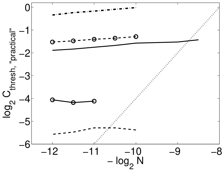
Figure 19: Dependence of the “practical” threshold, described before (7.4b), on $N^{-1}\propto\Delta x$. Solid, dashed, and (thicker) dash-dotted lines pertain to the initial conditions (7.1), (7.5), (7.6), and solid and dashed lines with circles pertain to initial conditions (7.2), (7.3), respectively. Dotted line: the slope predicted by (7.4b). The smallest $N$ in each case was dictated by ensuring a sufficiently small discretization error, whereas the largest, $N=2^{12}$, was used to constrain the computational time. Also, since for lower $N$ the growth rate of “sluggish” NI is non-monotonic in $C$ (feature(ii) in Sec. 5.3), we reported the largest observed $C_{\rm thresh,\,``practical"}$. (That is, for some $C$ below that value, NI may grow by more than on order of magnitude in $t=1000$, but a subsequent increase of $C$ will not necessarily lead to a stronger NI.)

8 Conclusions

8.1 Summary of results

The main contribution of this work is the development of the (in)stability analysis of the fd-SSM beyond the von Neumann (i.e., constant-coefficient) approximation. Our analysis is valid for spatially-varying, pulse-like background solutions of the generalized NLS. We showed that, as previously for the s-SSM [23], this is done via a modified equation — (3.15), (5.3b), or (6.4b), — derived for the Fourier modes that approximately satisfy the resonance condition

$$|\beta|k^{2}\Delta t=\pi.$$ (8.1)

Analyzing the (in)stability of the fd-SSM then proceeds similarly to the (in)stability analysis of nonlinear waves, i.e., by solving an eigenvalue problem with a spatially-varying potential. In view of this it is clear that properties of NI and, in particular, its threshold, depend on the simulated solution and thus cannot be expected to be universally applicable to all solutions. However, our NI analysis does provide an understanding of the mechanism and of generic features of the NI for broad classes of background solutions. Below we summarize such mechanisms and features for three classes of pulse-like solutions of the generalized NLS.

The first such a class includes, as a prominent representative, the standing soliton of the pure NLS (1.2). Note that the corresponding modified equation for the numerical error, Eq. (3.15), is different from the analogous modified equation, (1.14), for the s-SSM. Their analyses are also qualitatively different, and so are the modes that are found to cause the instability of these two numerical methods. For the s-SSM, these modes are almost monochromatic (i.e., non-localized) waves $\sim\exp(\pm ikx)$ that “pass” through the soliton very quickly. It is this scattering of those waves on the soliton that was shown [23] to lead to their instability. In contrast, for the fd-SSM considered in this work, the dominant unstable modes are stationary relative to the soliton. Moreover, they are localized at the sides, as opposed to the core, of the soliton. To our knowledge, such localized modes were not reported before in studies of instability of nonlinear waves.

It was straightforward to obtain an approximate threshold, (4.3) (where $C$ is given by (2.2)), beyond which NI may occur. Our simulations showed that an NI does indeed occur just slightly above that threshold. In this regard let us note that a qualitatively different expression for a bound of the NI threshold, given in (7.4b), was recently proved in [16] (see Eq. (2.9) there) by a completely different method. Our threshold (4.3), which satisfies (7.4a), is clearly greater for $\Delta x\ll 1$. Also, as we have demonstrated above, it is close to being sharp. On the downside, it is strictly valid only when the initial condition is infinitesimally close to the soliton. Indeed, in Sec. 7 we showed numerically that when the initial deviation from the soliton is not too small, the threshold value of $C$ may decrease compared to (4.3). The NI threshold obtained in [16] does not require the initial deviation from the soliton to be infinitesimal. Yet, as we have demonstrated in Secs. 2, 4, 5, and 7.2, it is only a conservative bound and certainly is not sharp.

In Sec. 5 we considered the generalized NLS with an external potential $\Pi(x)$, Eq. (5.1b), and have shown that NI on the background of its soliton may be similar to that of the standing soliton of the pure NLS (1.2). We have also identified situations when the NI for (5.1b) can be observed at different spatial locations, such as minima of $\Pi(x)$ (Sec. 5.1) or the center of the soliton (Sec. 5.2). We have not considered the generalized NLS (1.1) with a nonlinearity other than cubic, e.g., saturable. However, we believe that in that case, the NI follows one of the scenarios described in Secs. 2, 4, 5.1, or 5.2, as long as the external potential is not wider or substantially taller than the “internal” potential created by the soliton itself.

The second class of background solutions, which leads to a noticeably different NI behavior, are (quasi-)periodic in time solutions, discussed in Sec. 7. The same kind of NI, which we called “sluggish”, also occurs for stationary solitons of the generalized NLS (5.1b) in which the external potential is either wider or substantially taller (or both) than the “internal” potential $\gamma|U_{\rm sol}(x)|^{2}$; see Sec. 5.3. The distinguishing feature of the “sluggish” NI is that it can remain weak even when $C$ exceeds the NI threshold by several tens percent. The modes that cause “sluggish” NI are not localized (see Figs. 10 and 12(a,b)), in contrast to the most unstable modes on the background of the pure NLS soliton (see Fig. 5). Yet, they “hinge” on the pulse’s “tails” (see next paragraph). Other features of the “sluggish” NI are listed in Sec. 5.3.

Since the “sluggish” NI reported in Sec. 5.3 and the NI of the first subclass of background solutions are described by similar equations, (5.9) and (4.2), respectively, they are not unrelated. In fact, the NI of the standing soliton of the pure NLS also has a “sluggish” stage, where the most unstable mode is not localized and the NI growth rate is not a monotonic function of $C$; see Appendix C. However, that stage exists only in a narrow interval of $C$ values of about 1% past the NI threshold given by (4.3), whereas the “sluggish” NI reported in Sec. 5.3 exists over several tens percent past the NI threshold. Therefore, one reason why we have singled out the “sluggish” NI as a separate phenomenon is that it is likely to be noticed in routine simulations, whereas the behavior described in Appendix C is not. The other reason is that it is the “sluggish” NI that is observed for near-soliton and, more generally, oscillating background solutions.

The third type of background solutions that we considered, in Sec. 6, is the moving soliton with speed $S=O(1)$ of the pure NLS. In this case, NI develops in a manner different from that for the other two classes of background solutions. Namely, the corresponding unstable modes are not localized and also are not “pinned” to the soliton; see Fig. 13(b). Rather, they and the soliton pass through each other (repeatedly, due to the periodic boundary conditions of the computational domain), and the NI is a result of two such waves’ interaction mediated by the soliton. This mechanism is remotely similar to the NI mechanism for the s-SSM. The corresponding Eqs. (6.4b) have the form similar to that of Eqs. (3.9) in [23]. The difference between these two equations is that for the s-SSM, the unstable modes pass through the soliton very fast and hence interact with each other weakly. This is the reason behind the NI of the s-SSM being weak; it is related to the wavenumbers of the interacting modes, satisfying (8.1), being large, of order $O(1/\sqrt{\Delta t})$. On the other hand, the modes causing the NI of the fd-SSM about the moving soliton pass through the soliton with speed $S=O(1)$ and, moreover, are almost stationary relative to one another (their group velocities are close to zero). The weakness of the fd-SSM does not appear to be related to any physical parameter being small or large; see the discussion related to estimate (6.17).

In Sec. 6, we did not mention the NI threshold for the moving soliton. Let us comment on this issue now. Formally, from estimate (6.18a), one may conclude that such a threshold does not exist (i.e., the fd-SSM is, again, formally, unconditionally unstable). This is because for arbitrarily small $\Delta t$ (or, equivalently, $C$), there are always bands of wavenumbers $k$ where $|R|>1$ and hence the NI growth rate $\lambda>0$; see (6.18b) and (6.5). Less formally, even thought the continuous operator $i\partial_{z}$ in (6.7) is sign indefinite and unbounded, the corresponding operator on the discrete grid takes on values within the interval $[-k_{\max},\,k_{\max}]$. Then, following the reasoning that led to threshold (4.3), one could have obtained a threshold value of $\mu$, and hence $C$, below which NI of the moving soliton would be guaranteed not to occur. A simple estimate yields that in this case, one would find $C_{\rm thresh}=O(\Delta x)$ and hence $\Delta t_{\rm thresh}=O(\Delta x\,^{3/2})$. However, such an estimate is of no practical value. Indeed, we have repeatedly mentioned in Sec. 6 that our analysis there had overestimated the NI growth rate, and already for $C=0.7$ (and $K_{\rm sol}\approx 1$), the NI may take $t>1000$ to become just barely visible above the noise floor. For $C=0.5$, it takes several thousand time units to appear above the noise floor, and for a yet smaller $C$ it will take even longer. Thus, it is unlikely that such a weak NI could be significant in simulations.

8.2 Open problems

8.2.1 Analysis of (4.2) and (5.9) in the limit $\epsilon\rightarrow 0$

As we explained in Sec. 3, WKB solution of these eigenproblems would require the handling of the turning points where a pair of eigenvectors of the non-self-adjoint system of linear Schrödinger-type equations becomes linearly dependent. This appears to have been a long-standing unsolved problem (see, e.g., [30, 31]). Therefore, we find it reasonable to discuss only those aspects of (4.2) and (5.9) that do not require solving that problem.

Let us begin with (4.2). Figure 21 in Appendix C suggests that eigenvalues of the unstable modes at their “birth” satisfy $|\Lambda|\ll D$. The smallness of $|\Lambda|/D$ could be used to consider (4.2) as a perturbation of the WKB-solvable system (11.1b). This may explain the cascade of bifurcations that eventually leads to the emergence of a pair of real eigenvalues, resulting in NI. It may also give a value of the sharp NI threshold $C_{\rm cr}$, defined in Appendix C. It could also be interesting to find out how that cascade of bifurcations is affected by the size $L$ of the computational domain. Namely, as $L\rightarrow\infty$, will it “collapse” to a single value of $C$ where an unstable eigenmode, having once emerged, would persist for all greater values of $C$, as opposed to the behavior described in Appendix C?

With respect to (5.9), we sketch an approach by which the “sluggish” NI of a stationary soliton, described in Sec. 5.3, could be analyzed. As we mentioned there, the occurrence of “sluggish” NI requires that the external potential $\Pi(x)$ be substantially wider or taller than the “internal” one, $\gamma|U_{\rm sol}(x)^{2}|$. From Fig. 12 we notice that in such a case, the eigenmode overlaps much more with the external than with the “internal” potential. Therefore, the $\gamma|U_{\rm sol}(x)^{2}|$-term in (5.9) can be considered as a small perturbation. The remaining part of that eigenproblem decouples into two linear Schrödinger equations, which can be solved by the WKB method. Then the solution of (5.9) could be sought as a perturbation of that solution with $\gamma=0$. One of the features of “sluggish” NI, noted in Sec. 5.3, was that the most unstable mode is delocalized in a rather wide range of $C$ values past the NI threshold. As for (4.2), here it could also be interesting to find out how this is affected by the size of the computational domain. In other words, is “sluggish” NI a finite-$L$ phenomenon or will it persist on the infinite line?

8.2.2 Numerical instability of oscillating solutions

Recall that (3.14) describes the evolution of a high-$k$ numerical error with an arbitrary, including oscillatory, background $u_{\rm b}$. In Appendix D we argued that the standard technique of splitting the fields in (3.14) into slowly and rapidly varying parts does not appear to lead to an analytically tractable model. An alternative approach could, perhaps, be based on proper orthogonal decomposition of the background oscillating solution into a small number of rapidly diminishing “principal components”. For example, such a decomposition of solution (12.3) into just two principal components can be found in [37].

8.2.3 Numerical instability of moving soliton

We were unable to analytically solve Eqs. (6.4b) with $U_{\rm sol}(x)\propto{\rm sech}\,(x)$ and hence had to approximate it by a box profile. It is unclear whether an analytical solution with (6.4b) without such an approximation is even possible, except, perhaps, in the limit $\mu\rightarrow\infty$. However, that limit is of no practical interest since it corresponds to $C\rightarrow 0$, and we have noted that NI in that case is so weak that it may never be observed in simulations. Therefore, we do not propose solving the non-approximated (6.4b) as an open problem.

Instead, we think that obtaining an equation for a high-$k$ numerical error that could be valid for $0<S<O(1)$ is an interesting open problem. Such an equation must somehow account for the Fourier spectrum of the error having a structure seen in the three bottom curves in Fig. 17(b): a narrow peak (i.e., delocalized in $x$) on top of a broad pedestal (i.e., variations in $x$ on a scale much shorter than $O(1)$). At the moment we do not know how to approach that problem. If such an equation is obtained, its analysis, even only numerical, would be another interesting problem. Indeed, it would have to exhibit a transition of the unstable mode from being “pinned” to the soliton (for $S=0$) to passing through it (for $S=O(1)$).

Even more fundamental seems to be another issue, which lies at the heart of the difference between the modified equations of the high-$k$ numerical error for the standing and moving solitons, i.e., Eqs. (3.14) and (6.4b), respectively. This difference stems from that of the spectra of the numerical error in this two cases: a broad spectrum for the standing soliton (Fig. 2(a)) and rather narrow peaks for the moving one (Figs. 13(a) and 18(b)). Recall that Eqs. (3.14) and (6.4b) did not explain those differences; rather, they were derived based on the numerically observed different spectra. Thus, an open question is: How can one tell from the form of the background solution of the NLS what the spectrum of unstable modes of the fd-SSM should be?

8.2.4 Miscellaneous

We believe that analysis of NI of the SSM and related methods (e.g., the integrating factor method) is an unexplored area where techniques of stability analysis of nonlinear waves could be applied. As examples, let us mention just three broad topics, which were not considered in this work:  (i) NI of s- and fd-SSMs in two and three spatial dimensions;  (ii) NI of the generalized NLS (5.1b) where the external potential $\Pi(x)$ grows at infinity, e.g., $\Pi(x)\propto x^{2}$, as in the Gross–Pitaevskii equation;  (iii) NI of solitons in long-wave, e.g., Korteweg–de Vries, equations.

Appendix A: Modified linearized NLS for fd-SSM with non-periodic boundary conditions

We consider homogeneous Dirichlet boundary conditions (b.c.), which are compatible with the standing soliton solution of (1.2) in a large computational domain. Neumann or mixed b.c. can be treated similarly, and lead to similar results.

The equation for the dispersive step of the fd-SSM is still given by (1.6). However, now instead of (1.7) we assume: $u_{n+1}^{0}=0$, $u_{n+1}^{M}=0$, where $m=0$ and $m=M$ are the end points of the spatial grid. Then (1.6) can be rewritten as [38]

$$({\mathcal{I}}+(i\beta r/2){\mathcal{A}})\,{\bf u}_{n+1}=({\mathcal{I}}-(i\beta r/2){\mathcal{A}})\,{\bf\bar{u}},$$ (9.1)

where: ${\bf\bar{u}}=[\bar{u}^{1},\bar{u}^{2},\ldots,\bar{u}^{M-1}]^{T}$, similarly for ${\bf u}_{n+1}$, ${\mathcal{I}}$ is an $(M-1)\times(M-1)$ identity matrix, and ${\mathcal{A}}$ is an $(M-1)\times(M-1)$ tridiagonal matrix with $(-2)$ on the main diagonal and $(+1)$ on the sub- and super-diagonals.

The starting point of our derivation in Sec. 3, Eq. (3.1), has exacly the same form for the case of the Dirichlet b.c., except that ${\mathcal{F}}$ is replaced with ${\mathcal{T}}$ — an expansion over the complete set of the eigenvectors of ${\mathcal{A}}$; similarly, ${\mathcal{F}}^{-1}$ is replaced by ${\mathcal{T}}^{-1}$. The exponential in (3.2) that acts on the $j$th eigenvector is replaced by

$$e^{iP_{j}}=\frac{1-i\beta r\lambda_{j}/2}{1+i\beta r\lambda_{j}/2},$$ (9.2)

where $\lambda_{j}$ is the corresponding eigenvalue [38]:

$$\lambda_{j}=-4\sin^{2}\big{(}\pi j/(2M)\big{)}.$$ (9.3)

Equations (9.2), (9.3) and the middle expression in (3.2) coincide provided that we identify:

$$k=j\pi/(M\Delta x)=j\pi/L.$$ (9.4)

However, we are still a step away from proving that the modified linearized NLS for the Dirichlet b.c. case is the same as that equation for periodic b.c.. This is because $-k^{2}$, which is the Fourier symbol of the second derivative, is not the symbol of the second derivative under the transformations ${\mathcal{T}}$ and ${\mathcal{T}}^{-1}$. Under those transformation, the required symbol is given by (9.3). We will now use this observation to supply the last step and show that the modified linearized NLS for the case of Dirichlet b.c. is indeed the same as (3.14). This follows from (9.2)–(9.4) and a calculation that is similar to (3.4):

$$e^{iP(k)} \approx -\left(1+\frac{1}{i\beta r\big{(}1-\sin^{2}((k-k_{\max})\Delta x/2)\big{)}}\right)$$ (9.5)

$$\approx -\left(1+\frac{1}{i\beta r}+\frac{\sin^{2}((k-k_{\max})\Delta x/2)\big{)}}{i\beta r}\right),$$

where we have used that $\sin(k_{\max}\Delta x/2)=1$ and that for highly oscillatory eigenvectors of ${\mathcal{A}}$, one has $(k-k_{\max})\Delta x\ll 1$. The last term on the r.h.s. of (9.5) is the desired symbol of the second derivative, and then the rest of the derivation is the same as that leading to (3.11). From it one obtains the same modified linearized NLS as (3.14). Our numerical simulations of the NLS using the fd-SSM with zero Dirichlet b.c. confirm this conclusion.

Appendix B: Numerical solution of eigenproblem (4.2)

We work with (4.2) written in an equivalent form:

$$\sigma_{3}\left(\partial_{X}^{2}+D-V(\epsilon X)\left(\begin{array}[]{cc}2&1\\ 1&2\end{array}\right)-i\Lambda_{0}\sigma_{3}\,\right)\vec{\phi}\,=\,i(\Lambda-\Lambda_{0})\vec{\phi},$$ (10.1)

where the reason to include a constant $\Lambda_{0}$ will be explained later. We discretize (10.1) using Numerov’s method, which approximates the equation  $\Phi_{XX}=F(\Phi,X)$  by a finite-difference scheme

$$\Phi^{m+1}-2\Phi^{m}+\Phi^{m-1}=\frac{\Delta X\,^{2}}{12}\big{(}F^{m+1}+10F^{m}+F^{m-1}\big{)}$$ (10.2)

with accuracy $O(\Delta X\,^{4})$. Here $\Phi^{m}\equiv\Phi(X_{m})$, $F^{m}\equiv F(\Phi^{m},X_{m})$, etc., and $m=1,\ldots\,,\bar{M}-1$. Note that the number of grid points, $\bar{M}$, in the $X$-domain is much greater than the number of grid points, $M$, in the $x$-domain, because $X\propto x/\epsilon$; see (4.1), (3.10). Then, for the discretized solution ${\bf f}_{k}=[\phi_{k}^{1},\ldots\,,\,\phi_{k}^{\bar{M}-1}]^{T}$ ($k=1,2$) one obtains:

$$(-1)^{k-1}\left(\,\left[\frac{1}{\Delta X\,^{2}}{\mathcal{A}}_{\rm per}+{\mathcal{N}}_{\rm per}\left\{D{\mathcal{I}}-2{\mathcal{V}}-i\Lambda_{0}(-1)^{k-1}{\mathcal{I}}\right\}\right]{\bf f}_{k}\,-\,{\mathcal{N}}_{\rm per}{\mathcal{V}}{\bf f}_{3-k}\,\right)\,=\,i(\Lambda-\Lambda_{0}){\mathcal{N}}_{\rm per}{\bf f}_{k}.$$ (10.3)

Here all matrices, denoted by script letters, have size $(\bar{M}-1)\times(\bar{M}-1)$; ${\mathcal{I}}$ is defined after (9.1);  ${\mathcal{A}}_{\rm per}$ is as in (9.1) except that its $(1,\bar{M}-1)$th and $(\bar{M}-1,1)$th entries equal 1 (to account for the periodic boundary conditions);  ${\mathcal{N}}_{\rm per}$ has a similar structure as ${\mathcal{A}}_{\rm per}$:  $({\mathcal{N}}_{\rm per})_{m,m}=10/12$ (see (10.2)), $({\mathcal{N}}_{\rm per})_{(m-1),m}=({\mathcal{N}}_{\rm per})_{m,(m-1)}=1/12$, $({\mathcal{N}}_{\rm per})_{1,(\bar{M}-1)}=({\mathcal{N}}_{\rm per})_{(\bar{M}-1),1}=1/12$, and the rest of its entries are zero;  and ${\mathcal{V}}={\rm diag}(V^{1},\ldots\,,\,V^{\bar{M}-1})$. Next, defining the combined vector and matrices:

$$\hat{\bf f}=\left[\begin{array}[]{c}{\bf f}_{1}\\ {\bf f}_{2}\end{array}\right],\quad\hat{\mathcal{A}}_{\rm per}=\left(\begin{array}[]{cc}{\mathcal{A}}_{\rm per}&{\mathcal{O}}\\ {\mathcal{O}}&{\mathcal{A}}_{\rm per}\end{array}\right),\quad\hat{\mathcal{N}}_{\rm per}=\left(\begin{array}[]{cc}{\mathcal{N}}_{\rm per}&{\mathcal{O}}\\ {\mathcal{O}}&{\mathcal{N}}_{\rm per}\end{array}\right),$$

$$\hat{\mathcal{V}}=\left(\begin{array}[]{cc}2{\mathcal{V}}&{\mathcal{V}}\\ {\mathcal{V}}&2{\mathcal{V}}\end{array}\right),\quad\hat{\sigma}_{3}=\left(\begin{array}[]{cc}{\mathcal{I}}&{\mathcal{O}}\\ {\mathcal{O}}&-{\mathcal{I}}\end{array}\right),$$

where ${\mathcal{O}}$ is the $(\bar{M}-1)\times(\bar{M}-1)$ zero matrix, one rewrites (10.3) as:

$$\hat{\sigma}_{3}\left[\frac{1}{\Delta X\,^{2}}\hat{\mathcal{A}}_{\rm per}+D\hat{\mathcal{N}}_{\rm per}-\hat{\mathcal{N}}_{\rm per}\hat{\mathcal{V}}-i\Lambda_{0}\hat{\sigma}_{3}\hat{\mathcal{N}}_{\rm per}\right]\hat{\bf f}\,=\,i(\Lambda-\Lambda_{0})\hat{\mathcal{N}}_{\rm per}\hat{\bf f}\,.$$ (10.4)

This equation has the form of the generalized eigenvalue problem ${\mathcal{G}}\hat{\bf f}=\lambda{\mathcal{H}}\hat{\bf f}$ where ${\mathcal{H}}=\hat{\mathcal{N}}_{\rm per}$ is a positive definite matrix. This problem can be solved by Matlab’s command eigs. As its options, we specified that 108 smallest-magnitude eigenvalues and the corresponding eigenmodes needed to be computed. Among them, we looked only at those with complex $\Lambda$. Beyond the instability threshold there are several such modes. We visually inspected them and found that the most unstable mode was also the most localized and also had a real eigenvalue.

We verified that the eigenvalues did not change to five significant figures whether we used $\Delta X=1/10$ or $1/20$; so we used $\Delta X=1/10$. Finally, for relatively large $D\geq 0.1$, it was convenient to shift the eigenvalues by some $\Lambda_{0}$ (found at a previously considered value of $D$), so that those with largest $\Lambda_{R}$ would appear at the beginning of the list, when they are sorted by Matlab according to their absolute value in ascending order.

Appendix C: “Birth” of localized unstable mode

The instability growth rates plotted in Fig. 3 are monotonic functions of the parameter $C$. This, however, occurs only when $C$ is sufficiently beyond a critical value, $C_{\rm cr}$, where the dominant (i.e., with the greatest-$|\Lambda_{R}|$) unstable mode is created. Near $C_{\rm cr}$, which is slightly above the threshold value given by the r.h.s. of (4.3), the evolution of the greatest-$|\Lambda_{R}|$ eigenvalue is quite irregular.

Below we present results about this evolution for the dominant unstable mode (shown in Fig. 5) for $L=40$, $N=2^{9}$ (i.e., $\epsilon=40/1024\approx 0.04$) and the rest of the parameters being the same as listed in Sec. 2, i.e.: $\beta=-1$, $\gamma=2$, and $A=1$. Then, parameters $C$ and $D$ are related by (4.6): $D=C-1$. While we have been unable to rigorously establish an analytical expression for $C_{\rm cr}$, we will present a hypothesis as to what it may be. The main message that we intend to convey is that the “birth” of a localized eigenmode of Eq. (4.2) occurs via a complex sequence of bifurcations, in contrast to a single bifurcation that typically takes place when an unstable mode of a nonlinear wave is “born” (see, e.g., [39]).

We numerically observed that eigenmodes of (4.2) with $\Lambda_{R}\neq 0$ are “born” in two ways. One is when two imaginary eigenvalues $\pm i\Lambda_{I}$ “collide” at the origin (i.e., $\Lambda_{I}\rightarrow 0$) and thereby give rise to two real ones. The other way is a “collision” of two imaginary eigenvalues $i\Lambda_{I1}$ and $i\Lambda_{I2}$ away from the origin (i.e., $i\Lambda_{I1}\rightarrow i\Lambda_{I2}\neq 0$). In that case two complex eigenvalues are “born”. The very first (i.e., for the smallest $C$) unstable mode is created in the former way. We will now show that this mode is essentially non-localized and, moreover, it is not the mode that eventually becomes the dominant unstable mode, whose growth rate is plotted in Fig. 3. The reason why we still chose to discuss the former mode while being primarily interested in the latter one, will become clear as we proceed.

For a mode with $\Lambda=0$, Eq. (4.2) can be split into two uncoupled linear Schrödinger equations:

$$\big{(}\,\partial_{X}^{2}+D-\nu_{\pm}\,V(\epsilon X)\,\big{)}\phi_{\pm}=0,\qquad\phi_{\pm}=\phi_{1}\pm\phi_{2},$$ (11.1a)

where $$\nu_{-}=1 \nu_{+}=3 \phi_{\pm}$$ and . Note that satisfy the periodic boundary conditions:

$$\phi_{\pm}(-L/(2\epsilon))\,=\,\phi_{\pm}(L/(2\epsilon)).$$ (11.1b)

In Fig. 20(a) we show an example of a nontrivial solution of (11.1b). In view of the periodic boundary conditions, this figure is equivalent to Fig. 20(b). Recall from Sec. IV that the eigenmode is exponentially small inside the soliton. Then the solution shown in Fig. 20(b) can be thought of as being localized inside the valley bounded by the two “halves” of the potential. Using this observation, one can estimate the isolated values of $D$ for which one of the equations (11.1a), along with (11.1b), has a nontrivial solution, by the standard WKB method. The condition for the existence of a mode localized inside the valley of Fig. 20(b) is given by the Bohr–Sommerfeld formula:

$$\left(\int_{-L/(2\epsilon)}^{X_{\rm left}}+\int_{X_{\rm right}}^{L/(2\epsilon)}\right)\,\sqrt{D-\nu V(\epsilon X)}\,dX\,=\,\pi\left(n+\frac{1}{2}\right),$$ (11.2)

where $\nu$ is either $\nu_{-}$ or $\nu_{+}$, $n$ is an integer, and $X_{\rm left,\,right}$ are the turning points (see Sec. 4), where

$$D-\nu V(\epsilon X_{\rm left,\,right})=0.$$ (11.3)

The number of full oscillation periods of the mode inside the valley equals $n$; for example, in Fig. 20, $n=3$.

 

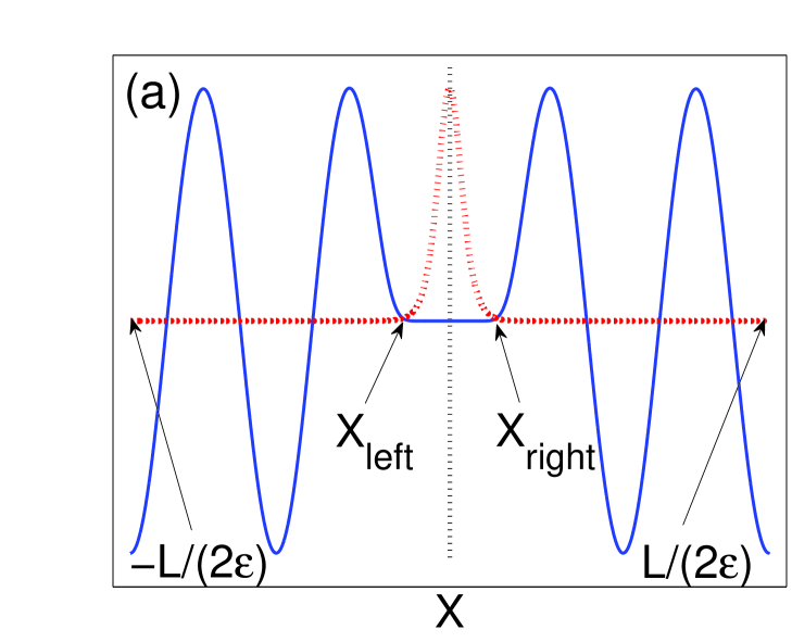
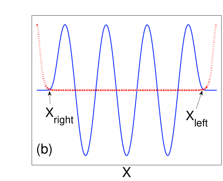
Figure 20: (Color online)  (a): A solution of (11.1b) (solid); potential ${\rm sech}\,^{2}(\epsilon X)$ (red dotted). The amplitude of the solution is normalized to that of the potential.  (b): Same as (a), but that panel is “cut” along the vertical dotted line at the center, and the resulting halves are interchanged.

When $D\ll 1$, the ${\rm sech}\,^{2}$ potential in (11.3) can be approximated by an exponential:  ${\rm sech}\,^{2}(\epsilon X)\approx 4\exp(-2\epsilon X)$. Then, using (4.1) and (11.3), we reduce (11.2) to

$$\sqrt{D}\int_{X_{\rm right}}^{L/(2\epsilon)}\sqrt{1-\exp[-2\epsilon(X-X_{\rm right})]}\,dX\,=\,\frac{\pi}{2}\left(n+\frac{1}{2}\right),$$ (11.4)

with $X_{\rm left}=-X_{\rm right}$ and

$$X_{\rm right}=\frac{1}{2\epsilon}\,\ln\frac{8\nu C\beta^{2}}{D}\,.$$ (11.5)

Neglecting the exponentially small terms of the order $O\big{(}\,\exp[-(L-2\epsilon X_{\rm right})]\,\big{)}$, one obtains from (11.4):

$$\sqrt{D}\left(L-\ln\frac{8\nu C\beta^{2}}{D}-2(1-\ln 2)\right)=\epsilon\,\pi\left(n+\frac{1}{2}\right).$$ (11.6)

Note that the WKB condition (11.2), and hence (11.6), is valid when $n$ is sufficiently large. In particular, it is not supposed to accurately predict the “birth” of the first unstable mode, where $n=0$. Indeed, Eq. (11.6) predicts that such a mode (for $\nu=1$) emerges at $D\approx 5.9\cdot 10^{-6}$, while numerically (see Appendix B) it is found at $D\approx 1.6\cdot 10^{-5}$. (A similar mode for $\nu=3$ emerges at a slightly higher value of $D$.) Formula (11.6) becomes accurate to the fourth significant figure in $D$ for $n\gtrsim 20$.

As we noted above, the first unstable mode is not the one that eventually becomes the dominant unstable mode. It disappears already at $D\approx 1.7\cdot 10^{-5}$, and there is an adjacent interval of $D$ values where all the eigenvalues of (4.2) are purely imaginary (i.e., the soliton is numerically stable). As $D$ increases, higher-order “real” (i.e., with $\Lambda_{I}=0$) modes appear and disappear in a similar fashion, as do quadruplets of modes with complex $\Lambda$. In both these types of modes, $\Lambda_{R}$ is fairly small: $|\Lambda_{R}|\lesssim D/10$. There also exist intervals of $D$, of increasingly small length, where all $\Lambda$’s are purely imaginary. This situation persists until the dominant unstable mode appears at $D_{\rm cr}\,(=C_{\rm cr}-1)$. This occurs as follows.

First, at $D\approx 0.012134$, a “real” mode appears (see Fig. 21(a,b)), and from this point on there always exists a “real” mode, even though the particular mode “born” at $D\approx 0.012134$ disappears later on. Specifically, at $D\approx 0.012928$, another “real” mode acquires $\Lambda_{R}$ greater than that of the mode “born” at $D\approx 0.012134$, and the latter mode soon disappears (Fig. 21(c,d)). A similar switchover between “real” modes occurs at least one more time near $D\approx 0.013750$ (not shown). Next, another “real” mode is “born” via a cascade of bifurcations near $D\approx 0.0162$ (Fig. 21(e,f)), and its $\Lambda_{R}$ crosses that of the previously dominant-$\Lambda_{R}$ “real” mode near $D\approx 0.01635$. At $D=0.0170$, these two dominant “real” modes have $\Lambda_{R}\approx 1.4\cdot 10^{-3}$ and $1.5\cdot 10^{-3}$ (Fig. 21(e)). Finally, these two modes gradually approach each other while crossing at least once more near $D=0.01725$. At $D=0.023$ and beyond, their eigenvalues are the same to five significant figures. Thus, remarkably, the dominant unstable mode eventually becomes doubly degenerate. We verified that such a degeneracy also occurs for the higher-order localized unstable modes, shown in Fig. 7.

   

   

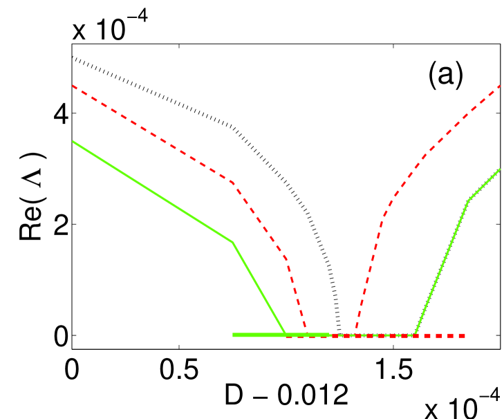
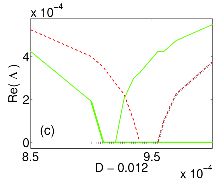
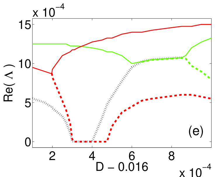
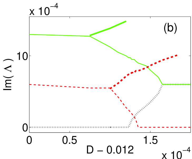
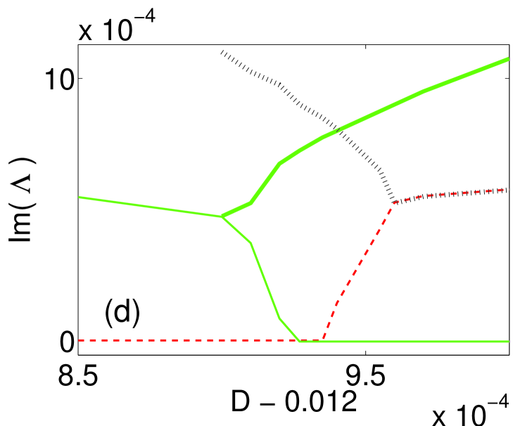
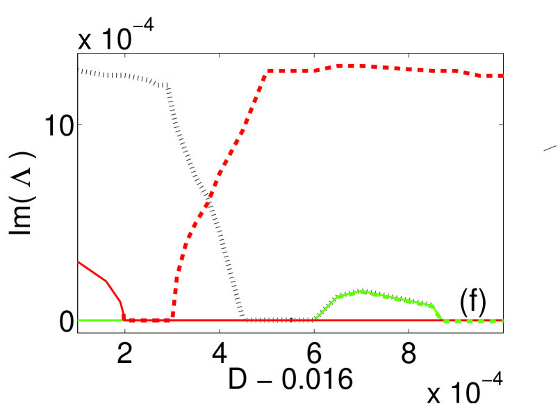
Figure 21: (Color online)  Real and imaginary parts of selected modes of (4.2), including the most unstable mode.  (a) & (b): $0.01200\leq D\leq 0.01220$;  (c) & (d): $0.01285\leq D\leq 0.01300$;  (e) & (f): $0.01610\leq D\leq 0.01700$. Same line colors, styles, and widths are used to indicate the same modes within one pair of panels (e.g., (c) & (d)). The same line colors/styles/widths in different pairs of panels (e.g., in (a) & (b) and (c) & (d)) do not imply the same modes.

To conclude, we present a hypothesis as to why the value $C_{\rm cr}$, where a “real” mode appears permanently (see above), is near $C=1.013$. Let us interpret (11.6) in a way that the $n$ on its r.h.s. is not necessarily an integer, but a continuous function of the parameter $D$. For those values of $D$ when $n$ is an integer, a mode with a real $\Lambda$ either appears or disappears at the origin $\Lambda=0$. Evaluating $n$ at the values of $D$ listed in the previous paragraph in connection with Figs. 21(a)–(d), one finds:

$$\underline{{\rm at}\;\;D=0.012134}: n|_{\nu=1}\approx 29.02,\qquad n|_{\nu=1}-n|_{\nu=3}\approx 0.99;$$ (11.7a)

$$\underline{{\rm at}\;\;D=0.012928}: n|_{\nu=1}\approx 30.02,\qquad n|_{\nu=1}-n|_{\nu=3}\approx 1.02;$$ (11.7b)

$$\underline{{\rm at}\;\;D=0.013750}: n|_{\nu=1}\approx 31.04,\qquad n|_{\nu=1}-n|_{\nu=3}\approx 1.05.$$ (11.7c)

That is, both $n|_{\nu=1}$ and $n|_{\nu=3}$ are simultaneously very close to integers. At $D=0.012928$, one of the “real” modes has not yet disappeared while the next one has appeared (Fig. 21(c)). From (11.7) we observe that at this value of $D$, the difference $(n|_{\nu=1}-n|_{\nu=3})$ exceeds $1$ for the first time. Thus, we hypothesize that $C_{\rm cr}\equiv 1+D_{\rm cr}$ is found from the condition that $(n|_{\nu=1}-n|_{\nu=3})$ exceeds $1$ for the first time. Verification of this hypothesis requires a deeper analytical insight than we have at the moment. Moreover, finding a value of $C$ past which the dominant real eigenvalue increases monotonically (as seen in Fig. 21(e)) is also an open question.

Appendix D: Possible reason behind “sluggish” numerical instability of oscillating pulse

Here we will give an argument in favor of a relation between mechanisms of “sluggish” NI for a stationary pulse in a potential (Sec. 5.3) and for an oscillating pulse (Sec. 7). The key observation here is that the (approximate) period of the oscillations, which is $O(1)$, is much smaller than the characteristic time over which NI develops, which is $O(100)$ and greater. This allows one to invoke well-known techniques of analysis of the evolution with rapidly oscillating perturbations in solving Eq. (3.14). Specifically, we split the background $u_{\rm b}^{2}$ and the solution $\tilde{w}$ into slowly (‘s’) and rapidly (‘r’) varying parts:

$$u_{\rm b}^{2}=\left(\varrho_{s}+\varrho_{r}\right)\,e^{2i[\vartheta_{s}+\vartheta_{r}]},$$ (12.1a)

where all the variables are real-valued and depend on $$x t$$ and , and

$$\tilde{w}=\left(\zeta_{s}+\zeta_{r}\right)\,e^{i[\vartheta_{s}+\vartheta_{r}]},$$ (12.1b)

where now $\zeta_{s,r}$ may be complex. In what follows we will denote $\partial_{t}\vartheta_{s,r}\equiv\dot{\vartheta}_{s,r}$ and $\partial_{\chi}\vartheta_{s,r}\equiv\vartheta\,^{\prime}_{s,r}$. Substitution of (12.1b) into (3.14) and separation of the slow and fast parts yields:

$$i\zeta_{s,\,t} +\left(\Gamma\big{(}1+(\vartheta_{s}^{\prime})^{2}-i\vartheta_{s}^{\prime\prime}\big{)}-\dot{\vartheta}_{s}\right)\zeta_{s}-2i\Gamma\vartheta_{s}^{\prime}\zeta_{s,\,\chi}-\Gamma\zeta_{s,\,\chi\chi}+\gamma\varrho_{s}(2\zeta_{s}+\zeta_{s}^{*})$$ (12.2a)

$$+\left\langle\left(\Gamma\big{(}\,2\vartheta_{r}^{\prime}\vartheta_{s}^{\prime}-i\vartheta_{r}^{\prime\prime}\big{)}-\dot{\vartheta}_{r}\right)\zeta_{r}-2i\Gamma\vartheta_{r}^{\prime}\zeta_{r,\,\chi}+\gamma\varrho_{r}(2\zeta_{r}+\zeta_{r}^{*})\right\rangle\;=\;0;$$

$$i\zeta_{r,\,t} +\left(\Gamma\big{(}1+(\vartheta_{s}^{\prime})^{2}-i\vartheta_{s}^{\prime\prime}\big{)}-\dot{\vartheta}_{s}\right)\zeta_{r}-2i\Gamma\vartheta_{s}^{\prime}\zeta_{r,\,\chi}-\Gamma\zeta_{r,\,\chi\chi}+\gamma\varrho_{s}(2\zeta_{r}+\zeta_{r}^{*})$$ (12.2b)

$$+\left\{\left(\Gamma\big{(}\,2\vartheta_{r}^{\prime}\vartheta_{s}^{\prime}-i\vartheta_{r}^{\prime\prime}\big{)}-\dot{\vartheta}_{r}\right)\zeta_{s}-2i\Gamma\vartheta_{r}^{\prime}\zeta_{s,\,\chi}+\gamma\varrho_{r}(2\zeta_{s}+\zeta_{s}^{*})\right\}\;=\;0.$$

Here $\Gamma\equiv 1/(C|\beta|)$ and $\langle\ldots\rangle$ denotes averaging over time; as usual, we have omitted terms that oscillate faster than (e.g., twice as fast as) $\vartheta_{r}$ and $\zeta_{r}$. The standard method is to solve (12.2b) for $\zeta_{r}$ and substitute the result in the second line of (12.2a). Solving (12.2b) analytically requires the assumption $|\zeta_{r}|\ll|\zeta_{s}|$, which, upon some calculations, reduces the terms in the second line of (12.2a) to $\langle\vartheta_{r}\varrho_{r}\rangle\zeta_{s}^{*}$, etc.. We numerically computed $\langle\vartheta_{r}\varrho_{r}\rangle$ for some of the solutions considered in Sec. 7 and found that it is considerably smaller than, e.g., $\varrho_{s}$. Therefore, we believe that the occurrence of “sluggish” NI for oscillating pulses is primarily related to terms in the first line of (12.2a).

We will argue this point using the solution generated by initial condition (7.2) as an example. The analytical form of this solution is

$$u(x,t)=\frac{\displaystyle 4e^{it}\left(\cosh(3x)+3e^{8it}\cosh(x)\right)}{\cosh(4x)+4\cosh(2x)+3\cos(8t)};$$ (12.3)

its snapshots are shown in Fig. 22(a). In Fig. 22(b) we show $\dot{\vartheta}_{s}$, computed as $\langle\dot{\vartheta}\rangle$. At the far “tails” of the pulse ($|x|>7$) the graph is irregular since the numerical error dominates over the solution (12.3). The important feature to note in Fig. 22(b) is that $\dot{\vartheta}_{s}$ is piecewise constant where $|u|^{2}$ is essentially nonzero. Thus, the corresponding term in the first line of (12.2a) creates an effective potential, which is one reason why NI in this case may be related to that described in Sec. 5.3. We emphasize that the piecewise-constant shape of $\dot{\vartheta}_{s}$ is common for all time-periodic (or almost periodic) solutions that we have simulated, e.g., that generated by initial condition (7.3). For quasi-periodic oscillating pulses, the transition region connecting one constant value of $\dot{\vartheta}_{s}$ to another or to the outside region is smooth rather than abrupt; see Fig. 22(c).

   

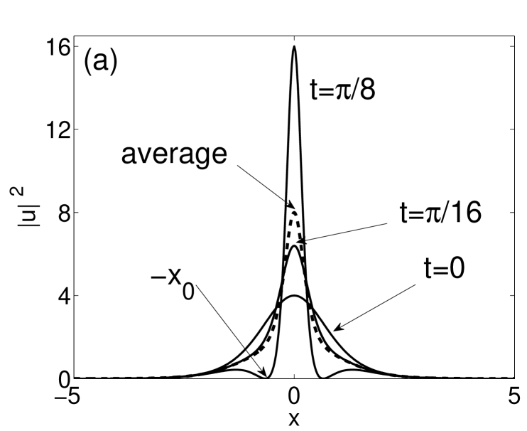
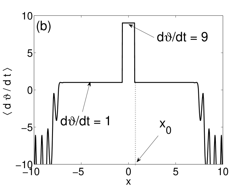
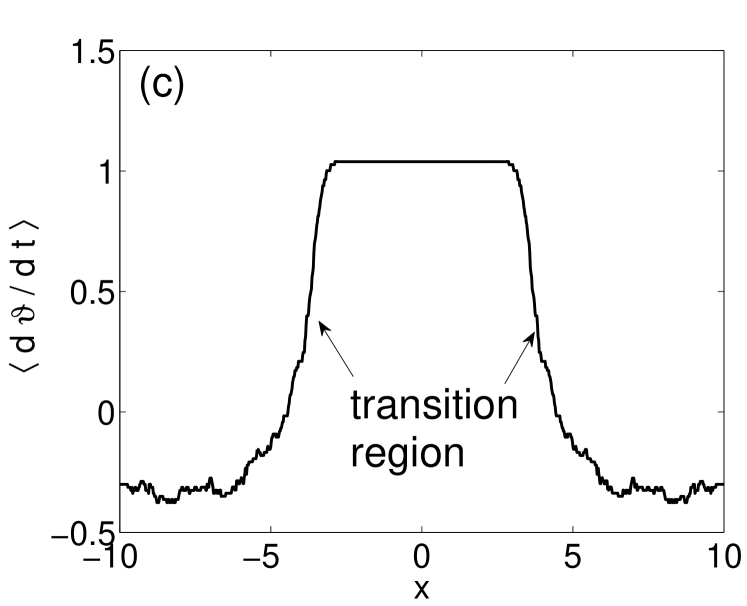
Figure 22: (a)  Snapshots and the average value of $|u|^{2}$ from (12.3).  (b)  $\dot{\vartheta}_{s}$ of the same solution.  In both panels, $x_{0}={\rm arcsinh}(1/\sqrt{2})$ is where $u(x_{0},\pi/8)=0$ and hence the phase has a discontinuity.  (c)  $\dot{\vartheta}_{s}$ of the solution generated by initial condition (7.6).

However, the reason presented in the previous paragraph may not be the only one behind the development of “sluggish” NI. Two other terms in the same equation, $\big{(}(\vartheta_{s}^{\prime})^{2}-i\vartheta_{s}^{\prime\prime}\big{)}$, create an additional, time-dependent, effective potential. Indeed, while $\vartheta_{s}^{\prime}=0$ wherever $\dot{\vartheta}_{s}={\rm const}$ with respect to $x$, it is nonzero in the transitional region. Since in that region $\dot{\vartheta}_{s}={\rm const}$ with respect to $t$, then $\vartheta_{s}^{\prime}\propto t$ there. Let us note that while $\partial_{x}\vartheta_{s}\sim\delta(x-x_{0})$, where $x_{0}$ is the location of the sharp transition region (see Fig. 22(b)), $\vartheta_{s}^{\prime}\equiv\partial_{\chi}\vartheta_{s}=\epsilon\partial_{x}\vartheta_{s}$ is a function varying on the scale $O(1)$ in $\chi$. Unfortunately, analytical solution of even simplest equations with time-dependent potential, like

$$iw_{t}+w_{xx}\pm t\,\delta(x)\,w=0,$$ (12.4)

does not appear to be possible. It is, therefore, an open problem to relate the development of “sluggish” NI of an oscillating pulse to some reduced model described by an equation of the form

$$iw_{t}+w_{xx}+\big{(}\Pi_{1}(x)w+\Pi_{2}(x)w^{*}\big{)}=0$$ (12.5)

for some time-independent $\Pi_{1}$ and $\Pi_{2}$. Such a model would generalize that considered in Secs. 3–5 and would be more amenable to standard methods of eigenvalue analysis than the time-dependent model discussed above.

References

- [1] R.H. Hardin and F.D. Tappert, Applications of the split-step Fourier method to the numerical soltion of nonlinear and variable coefficient wave equations, SIAM Review (Chronicle) 15, 423 (1973).
- [2] T. Taha and M. Ablowitz, Analytical and numerical aspects of certain nonlinear evolution equations. II. Numerical, Nonlinear Schrodinger equation, J. Comp. Phys. 55, 203–230 (1984).
- [3] G.P. Agrawal, Nonlinear fiber optics, 3rd Ed. (Academic Press, San Diego, 2001).
- [4] W. Bao and H. Wang, An efficient and spectrally accurate numerical method for computing dynamics of rotating Bose–Einstein condensates, J. Comput. Phys. 217, 612–626 (2006).
- [5] A.D. Bandrauk and H. Shen, Exponential split operator methods for solving coupled time-dependent Schrödinger equations, J. Chem. Phys. 99, 1185–1193 (1993).
- [6] E. Lorin, S. Chelkowski, A. Bandrauk, A numerical Maxwell–Schrödinger model for intense laser–matter interaction and propagation, Comput. Phys. Commun. 177, 908–932 (2007).
- [7] D. Lanser and J.G. Verwer, Analysis of operator splitting for advection–reaction–diffusion problems from air pollution modelling, J. Comp. Appl. Math. 111, 201–206 (1999).
- [8] J. Carrayroua, R. Mosé, and P. Behra, Operator-splitting procedures for reactive transport and comparison of mass balance errors, J. Contamin. Hydrology 68, 239–268 (2004).
- [9] A. Chertock, A. Kurganov, and G. Petrova, Fast explicit operator splitting method for convection–diffusion equations, Int. J. Numer. Meth. Fluids 59, 309–332 (2009).
- [10] F. Blumenthal, H. Bauke, A stability analysis of a real space split operator method for the Klein–Gordon equation, J. Comput. Phys. 231, 454–464 (2012).
- [11] G. Strang, On the construction and comparison of difference schemes, SIAM J. Numer. Anal. 5 506–517 (1968).
- [12] M. Glassner, D. Yevick, and B. Hermansson, High-order generalized propagation techniques, J. Opt. Soc. Am. B 8, 413–415 (1991).
- [13] J.A.C. Weideman and B.M. Herbst, Split-step methods for the solution of the nonlinear Schrödinger equation, SIAM J. Numer. Anal. 23, 485–507 (1986).
- [14] A. Carena, V. Curri, R. Gaudino, P. Poggiolini, and S. Benedetto, A time-domain optical transmission system simulation package accounting for nonlinear and polarization-related effects in fiber, IEEE J. Sel. Areas Commun. 15, 751–764 (1997).
- [15] Q. Chang, E. Jia, and W. Sun, Difference schemes for solving the generalized nonlinear Schrödinger equation, J. Comp. Phys. 148, 397–415 (1999).
- [16] D. Bambusi, E. Faou, and B. Grébert, Existence and stability of solitons for fully discrete approximations of the nonlinear Schrödinger equation, Numer. Math. 123, 461–492 (2013).
- [17] X. Antoine, W. Bao, and C. Besse, Computational methods for the dynamics of the nonlinear Schrödinger/Gross–Pitaevskii equation, Comp. Phys. Commun. 184, 2621–2633 (2013).
- [18] G. Li, Recent advances in coherent optical communication, Adv. Opt. Photon. 1, 279–307 (2009).
- [19] V.M. Kenkre and D.K. Campbell, Self-trapping on a dimer: Time-dependent solutions of a discrete nonlinear Schrödinger equation, Phys. Rev. B 34, 4959–4961 (1986).
- [20] A.B. Aceves and J.-G. Caputo, Mode dynamics in nonuniform waveguide arrays: a graph Laplacian approach, J. Opt. 16, 035202 (2014).
- [21] J. Von Neumann and R.D. Richtmeyer, A method for the numerical calculation of hydrodynamic shocks, J. Appl. Phys. 21, 232–237 (1950).
- [22] L.N. Trefethen, Spectral methods in Matlab (SIAM, Philadelphia, 2001), Chap. 10.
- [23] T.I. Lakoba, Instability analysis of the split-step Fourier method on the background of a soliton of the nonlinear Schrödinger equation, Num. Meth. Part. Diff. Eqs. 28, 641–669 (2012).
- [24] L. Gauckler and C. Lubich, Splitting integrators for Nonlinear Schrödinger equations over long times, Found. Comput. Math. 10, 275–302 (2010).
- [25] D.J. Kaup, Perturbation theory for solitons in optical fibers, Phys. Rev. A 42, 5689–5694 (1990).
- [26] H.T. Tran, Stability of dark solitons: Linear analysis, Phys. Rev. A 46, 7319–7321 (1992).
- [27] D.E. Pelinovsky, Yu.S. Kivshar, and V.V. Afanasjev, Internal modes of envelope solitons, Physica D 116, 121–142 (1998).
- [28] I.M. Gelfand, Lectures on linear algebra (Interscience Publishers, New York, 1961), Sec. 15.
- [29] G. Chen and J. Zhou, Vibration and damping in distributed systems, vol. II (WKB and wave methods, vizualization and experimentation) (CRC Press, Boca Raton, 1993), Sec. 1.2.
- [30] S.A. Fulling, Adiabatic expansions of solutions of coupled secondorder linear differential equations. II, J. Math. Phys. 20, 1202–1209 (1979).
- [31] A.A. Skorupski, Phase integral approximation for coupled ODEs of the Schrödinger type, J. Math. Phys. 49, 053523 (2008).
- [32] T.I. Lakoba, J. Yang, A generalized Petviashvili iteration method for scalar and vector Hamiltonian equations with arbitrary form of nonlinearity, J. Comp. Phys. 226, 1668–1692 (2007).
- [33] M. Segev, G.C. Valley, B. Crosignani, P. DiPorto, A. Yariv, Steady-state spatial screening solitons in photorefractive materials with external applied field, Phys. Rev. Lett. 73, 3211–3214 (1994).
- [34] U. Ascher, Surprising computations, Appl. Numer. Math. 62, 1276–1288 (2012).
- [35] T.I. Lakoba, Instability of the split-step method for a signal with nonzero central frequency, J. Opt. Soc. Am. B 30, 3260–3271 (2013).
- [36] D.J. Kaup, T.I. Lakoba, Variational method: How it can generate false instabilities, J. Math. Phys. 37, 3442–3462 (1996).
-
[37]
J.N. Kutz, Computational Methods for Data Analysis,
online course:
http://courses.washington.edu/amath582/; Sec. 18. - [38] D.R. Kincaid, E.W. Cheney, Numerical analysis: Mathematics of scientific computing, 3rd Ed. (Brooks/Cole, Pacific Crove, CA, 2002), Sec. 9.1.
- [39] T. Kapitula and B. Sandstede, Instability mechanism for bright solitary-wave solutions to the cubic-quintic Ginzburg–Landau equation J. Opt. Soc. Am. B 15, 2757–2762 (1998).