Access Policy Design for Cognitive Secondary Users under a Primary Type-I HARQ Process

Abstract

In this paper, an underlay cognitive radio network that consists of an arbitrary number of secondary users (SU) is considered, in which the primary user (PU) employs Type-I Hybrid Automatic Repeat Request (HARQ). Exploiting the redundancy in PU retransmissions, each SU receiver applies forward interference cancelation to remove a successfully decoded PU message in the subsequent PU retransmissions. The knowledge of the PU message state at the SU receivers and the ACK/NACK message from the PU receiver are sent back to the transmitters. With this approach and using a Constrained Markov Decision Process (CMDP) model and Constrained Multi-agent MDP (CMMDP), centralized and decentralized optimum access policies for SUs are proposed to maximize their average sum throughput under a PU throughput constraint. In the decentralized case, the channel access decision of each SU is unknown to the other SU. Numerical results demonstrate the benefits of the proposed policies in terms of sum throughput of SUs. The results also reveal that the centralized access policy design outperforms the decentralized design especially when the PU can tolerate a low average long term throughput. Finally, the difficulties in decentralized access policy design with partial state information are discussed.

I Introduction

The advent of new technologies and services in wireless communication has increased the demand for spectrum resources so that the traditional fixed frequency allocation will not be able to meet these bandwidth requirements. However, most of the spectrum frequencies assigned to licensed users are under-utilized. Thus, cognitive radio is proposed to improve the spectral efficiency of wireless networks [2]. Cognitive radio enables licensed primary users (PUs) and unlicensed secondary users (SUs) to coexist and transmit in the same frequency band [3], [4]. For a literature review on spectrum sharing and cognitive radio, the reader is referred to [5]-[7]. In the underlay cognitive radio approach, the smart SUs are allowed to simultaneously transmit in the licensed frequency band allotted to the PU. The PU is oblivious to the presence of the SUs while the SU needs to control the interference it causes at the PU receiver.

HARQ, a link layer mechanism, is a combination of high-rate forward error-correcting coding (FEC) and ARQ error-control, and is employed in current technologies, including for example HSDPA and LTE. CRNs with an HARQ scheme implemented by the PU are addressed in [8]-[15]. [8], [9] and [10] show how to exploit the Type-I HARQ retransmissions implemented by the PU. [8] considers a cognitive radio network composed of one PU and one SU, and does not utilize interference cancelation (IC) at the SU receiver. [9] employs Type-I HARQ with an arbitrary number of retransmissions and applies backward and forward IC after decoding the PU message at the SU receiver. The network considered in [10] is similar to [8], where the SU is also allowed to selectively retransmit its own previous corrupted message and apply a chain decoding protocol to derive the SU access policy. [11] applies Type-II Hybrid ARQ with at most one retransmission, where the SU receiver tries to decode the PU message in the first time slot and, if successful, it removes this PU message in the second time slot to improve the SU throughput. The extension of the work in [11] to IR-HARQ with multiple rounds is addressed in [12], where several schemes are proposed. [13] proposes SU transmission schemes when the SU is able to infrequently probe the channel using the PU Type-II HARQ feedback with Chase combining (CC-HARQ). Exploiting primary Type-II HARQ in CRN has also been studied in [14] and [15]. Note that deriving the benefit from PU Type-I HARQ for designing an optimum access policy has been only addressed for CRNs with one SU in the literature, with the exception of our work in [1]. We have to notice that increasing the number of SUs and allowing them to access the channel cause more interference at the PU receiver and therefore decrease the PU throughput. In fact it is necessary to control the access of the SUs to the channel to constrain the PU throughput degradation.

In this paper, an optimum access policy for $N$ SUs is designed, which exploits the redundancy introduced by the Type-I HARQ protocol in transmitting copies of the same PU message and interference cancelation at the SU receivers. The aim is to maximize the average long term sum throughput of SUs under a constraint on the average long term PU throughput degradation. We assume that the number of transmissions is limited to at most $T$ and all SUs have a new packet to transmit in each time slot. Two design scenarios are considered: in the first one, SUs make a channel access decision jointly, whereas in the second scenario, each SU makes an independent decision and does not know whether or not the other secondary users access the channel. We call them respectively as centralized and decentralized scenarios. Noting the PU message knowledge state at each of the SU receivers and also the ARQ retransmission time, the $PU-SU_{1}-...-SU_{N}$ network is modeled using MDP and MMDP models [16], respectively in centralized and decentralized scenarios. Due to the constraint on the average long term PU throughput, we then have a constrained MDP (CMDP) and Constrained MMDP (CMMDP).

In the centralized case, the access policy in one state shows the joint probability of accessing and/or not accessing the channel by the SUs. Using [17] and [18], it follows that the optimal policy may be obtained from the solution of a corresponding LP problem. In the decentralized scenario, there is an access policy for each SU describing the probability of accessing the channel by that SU. It is noteworthy that we are interested in random access policies instead of only deterministic access policies. Hence, the optimum polices in the centralized case can not be directly applied to a decentralized scenario. To propose local optimum access policies for the CMMDP model, we employ Nash Equilibrium.

The simulation results demonstrate that due to the use of forward IC (FIC), a cognitive radio network converges to the upper bound faster as the number of SUs increases for large enough SNR of the channels from the PU transmitter to SU receivers. The results also reveal that our proposed centralized access policy design significantly outperforms the decentralized one when the average PU throughput constraint is low.

The paper is organized as follows. Following the system model in Section II, the rates and the corresponding outage probabilities are computed in Section III. Optimal access policies for $N$ SUs in centralized and decentralized scenarios are proposed respectively in Sections IV and V. The numerical results are presented in Section VI and an extension to the paper is discussed in Section VII. Finally, the paper is concluded in Section VIII.

II System Model

In the system we consider, there exist one primary and N secondary transmitters denoted by $PU_{tx}$, $SU_{tx1}$,…,$SU_{txN}$, respectively. These transmitters transmit their messages with constant power over block fading channels. In each time slot (one block of the channel), the channels are considered to be constant. The instantaneous signal to noise ratios of the channels $PU_{tx}\rightarrow PU_{rx}$, $PU_{tx}\rightarrow SU_{rxn}$, $SU_{txn}\rightarrow SU_{rxm}$, $SU_{txn}\rightarrow PU_{rx}$, $n,m\in\{1,...,N\}$ are denoted by $\gamma_{pp}$, $\gamma_{ps_{n}}$, $\gamma_{s_{n}s_{m}}$ and $\gamma_{s_{n}p}$, respectively. As an example, the system model with the mentioned channel SNRs for $N=2$ is depicted in Fig. 1.

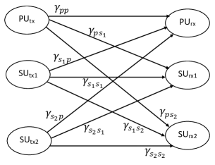
Figure 1: CRN Model with two SUs

We assume that no Channel State Information (CSI) is available at the transmitters except the ACK/NACK message and the PU message knowledge state. Thus, transmissions are under outage, when the selected rates are greater than the current channel capacity.

PU is unaware of the presence of the SUs and employs Type-I HARQ with at most $T$ transmissions of the same PU message. We assume that the ARQ feedback is received by the PU transmitter at the end of a time-slot and a retransmission can be performed in the next time-slot. Retransmission of the PU message is performed if it is not successfully decoded at the PU receiver until the PU message is correctly decoded or the maximum number of transmissions allowed, $T$, is reached . Fig. 2 shows the model of the PU Type-I HARQ, where $R_{P}$ is the PU transmission rate and $C_{t}$ is the capacity of the $PU_{tx}$ to $PU_{rx}$ channel in ARQ time slot $t$ when SU transmissions are considered as background noise at $PU_{rx}$. In each time-slot, each SU, if it accesses the channel, transmits its own message, otherwise it stays idle and does not transmit. This decision is based on the access policy described later. The activity of the SUs affects the outage performance of the PU, by creating interference at the PU receiver. The objective is to design access policies for SUs to maximize the average sum throughput of the SUs under a constraint on the PU average throughput degradation.

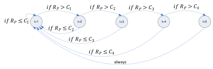
Figure 2: ARQ Type-I HARQ Model for $T=5$.

We consider centralized and decentralized scenarios. In the centralized scenario, there exists a central unit which receives the PU message knowledge states of the SUs as well as the ACK/NACK message from the PU receiver. This unit then computes the secondary access actions and provides them to the SUs. In the decentralized scenario, there exists no central unit. The PU message knowledge state at each SU receiver is fed back to all the SU transmitters, but each SU transmitter makes its own channel access decision independently, based on this information. Thus, in the decentralized design each SU is not aware of the access decisions of the other SUs in the same slot.

If $SU_{rxn}$, $n\in\{1,...,N\}$, succeeds in decoding the PU message, it can cancel it from the received signal in future retransmissions. We refer to this as FIC [9]. We call the PU message knowledge state as $\Phi=\bigl{(}\phi(1),...,\phi(N)\bigr{)}$, which belongs to the set of $2^{N}$ possible combinations of PU message knowledge states of all secondary users, where $\phi(n)$ is the PU message knowledge state of the $SU_{n}$ receiver. For example, if $\Phi=(K,K)$ for $N=2$, then $SU_{rx1}$ and $SU_{rx2}$ both know the PU message and thus can perform FIC.

In the centralized scenario, there are $2^{N}$ possible channel access combinations for the $N$ SUs, collected in the set $A=\{0,1,...,2^{N}-1\}$. Each action, denoted by $a$, can be represented as an $N$-dimensional vector $\Psi(a)=\bigl{(}\varphi(a,1),...,\varphi(a,N)\bigr{)}$ which is equal to the binary expansion of $a$, $0\leq a\leq 2^{N}-1$ and therefore, $\varphi(a,n)\in\{0,1\}$. Equivalently, we have

$$\Psi(a)=Dec2Bin_{N}(a),$$ (1)

where the function $Dec2Bin_{N}$ is the $N$-dimensional decimal to binary conversion. For access action $a$, $\varphi(a,n)=1$ means that $SU_{n}$ is allowed to access the channel. If $\Psi(a)=\mathbf{U}_{n}$, only $SU_{n}$ accesses the channel, where $\mathbf{U}_{n}$ is defined as follows:

Definition 1

$\mathbf{U}_{n}$ is an $N$-dimensional vector with $\mathbf{U}_{n}(n)=1$ and $\mathbf{U}_{n}(m)=0$ for $m\neq n$.

On the contrary, in the decentralized case, the access action is $a_{n}\in A_{n}=\{0,1\}$ for secondary user $n$, where $a_{n}=1$ means that this user is allowed to transmit.

III Rates and Outage Probabilities

First we consider the centralized scenario, where we have a joint access action $a\in A=\{0,1,...,2^{N}-1\}$ and then we address the decentralized scenario with independent $N$ access actions $a_{n}\in A_{n}=\{0,1\}$, $n\in{1,...,N}$.

III-A Centralized Scenario

The PU transmission rate, $R_{P}$, is considered fixed. However, based on the PU message knowledge state $\Phi$ and the access action $a$, the rate of each secondary user $n$ can be adapted and is denoted by $R_{s_{n},a,\Phi}$, $a\in A=\{1,...,2^{N}-1\}$. (All rates for access action $a=0$ are zero.)

The outage probability of the channel $PU_{tx}\rightarrow PU_{rx}$ for SU access action $a$ is denoted by $\rho_{p,a}$. Noting that the $SU_{n}$ transmissions $\forall n\in\{1,...,N\}$ are considered as background noise at $PU_{rx}$, we have

$$\rho_{p,a} =1-Pr\left(R_{p}\leq C(\frac{\gamma_{pp}}{1+\sum_{n=1}^{N}\varphi(a,n)\gamma_{s_{n}p}})\right)\;\;\;\;a\in A=\{0,1,...,2^{N}-1\},$$ (2)

where $C(x)=\log_{2}(1+x)$. Obviously, $C_{t}$ in Fig. 2 is equal to $C(\frac{\gamma_{pp}}{1+\sum_{n=1}^{N}\varphi(a,n)\gamma_{s_{n}p}})$ if in ARQ time $t$, action $a$ is selected.

The SNR region ${\Gamma}_{s_{n},a,\Phi}(R_{s_{1},a,\Phi},...,R_{s_{N},a,\Phi})$, $n\in\{1,...,N\}$, where $\phi(n)=K$, is the set of all $N-$tuples of $SNRs$ $(\gamma_{s_{1}s_{n}},...,\gamma_{s_{N}s_{n}})$, for which the $SU_{n}$ message transmitted at rate $R_{s_{n},a,{\Phi}}$ is successfully decoded at $SU_{rxn}$ regardless of the decoding of other SUs messages transmitted at rates $R_{s_{m},a,\Phi}$, $\forall m\neq n$. The SNR region $\dot{\Gamma}_{s_{n},a,\Phi}(R_{p},R_{s_{1},a,\Phi},...,R_{s_{N},a,\Phi})$ is similarly defined for $\phi(n)=U$ and contains all SNR vectors such that the $SU_{n}$ message transmitted at rate $R_{s_{n},a,{\Phi}}$ is successfully decoded at $SU_{rxn}$ irrespective of the decoding of other SUs and PU messages transmitted at rates $R_{s_{m},a,\Phi}$ and $R_{p}$ respectively. Thus, the outage probability of the channel $SU_{txn}\rightarrow SU_{rxn}$, $n\in\{1,...,N\}$ denoted by $\rho_{s_{n},a,\Phi}$ is computed as

$$\rho_{s_{n},a,\Phi=(\phi(1),...,\phi(n)=K,...,\phi(N))}=Pr\left((\gamma_{s_{1}s_{n}},...,\gamma_{s_{N}s_{n}})\notin{\Gamma}_{s_{n},a,\Phi}(R_{s_{1},a,\Phi},...,R_{s_{N},a,\Phi})\right)$$ (3)

and

$$\rho_{s_{n},a,\Phi=(\phi(1),...,\phi(n)=U,...,\phi(N))}=Pr\left((\gamma_{psn},\gamma_{s_{1}s_{n}},...,\gamma_{s_{N}s_{n}})\notin{\dot{\Gamma}}_{s_{n},a,\Phi}(R_{p},R_{s_{1},a,\Phi},...,R_{s_{N},a,\Phi})\right).$$ (4)

As an example of how the SNR regions can be determined, we have:

$${\dot{\Gamma}}_{s_{1},1,\Phi}(R_{p},R_{s_{1},1,\Phi})\overset{\Delta}{=}\biggl{\{}(\gamma_{s_{1}s_{1}},\gamma_{ps_{1}}):R_{s_{1},1,\Phi}\leq C(\gamma_{s_{1}s_{1}}),\biggr{.}$$

$$\biggl{.}\;R_{p}\leq C(\gamma_{ps_{1}}),R_{s_{1},1,\Phi}+R_{p}\leq C(\gamma_{s_{1}s_{1}}+\gamma_{ps_{1}})\biggr{\}}\bigcup$$

$$\biggr{\{}(\gamma_{s_{1}s_{1}},\gamma_{ps_{1}}):R_{p}>C(\gamma_{ps_{1}}),R_{s_{1},1,\Phi}\leq C(\frac{\gamma_{s_{1}s_{1}}}{1+\gamma_{ps_{1}}})\biggr{\}},\;\text{where }\phi(1)=U,$$ (5)

$${\Gamma}_{s_{1},3,\Phi}(R_{s_{1},3,\Phi},R_{s_{2},3,\Phi})\overset{\Delta}{=}\biggl{\{}(\gamma_{s_{1}s_{1}},\gamma_{s_{2}s_{1}}):R_{s_{1},3,\Phi}\leq C(\gamma_{s_{1}s_{1}}),\biggr{.}$$

$$\biggl{.}\;R_{s_{2},3,\Phi}\leq C(\gamma_{s_{2}s_{1}}),R_{s_{1},3,\Phi}+R_{s_{2},3,\Phi}\leq C(\gamma_{s_{1}s_{1}}+\gamma_{s_{2}s_{1}})\biggr{\}}\bigcup$$

$$\biggr{\{}(\gamma_{s_{1}s_{1}},\gamma_{s_{2}s_{1}}):R_{s_{2},3,\Phi}>C(\gamma_{s_{2}s_{1}}),R_{s_{1},3,\Phi}\leq C(\frac{\gamma_{s_{1}s_{1}}}{1+\gamma_{s_{2}s_{1}}})\biggr{\}},\;\text{where }\phi(1)=K.$$ (6)

As observed, ${\dot{\Gamma}}_{s_{1},1,\Phi}(R_{p},R_{s_{1},1,\Phi})$ depends on $R_{p}$ and $R_{s_{1},1,\Phi}$, when $\phi(1)=U$. This is because only $SU_{1}$ is allowed to access the channel when $a=1$ and the $PU$ message is unknown at $SU_{rx1}$. It is also seen that ${\Gamma}_{s_{1},3,\Phi}(R_{s_{1},3,\Phi},R_{s_{2},3,\Phi})$ depends on $R_{s_{1},3,\Phi}$ and $R_{s_{2},3,\Phi}$ when $\phi(1)=K$. The reason is that only $SU_{1}$ and $SU_{2}$ access the channel when $a=3$ and the $PU$ message can be removed at the $SU_{1}$ receiver. All other SNR regions can be similarly computed (full details for $N=2$ can be found in [19]).

III-B Decentralized Scenario

In the decentralized case, each SU does not coordinate its access action with the other SUs, and therefore there exist $N$ independent binary access actions $a_{n}\in A_{n}=\{0,1\}$ $\forall n\in\{1,...,N\}$. The access action $a$ in the decentralized case is the combination of $N$ binary decisions (actions) $a_{1},...,a_{N}$ and may be derived as follows:

$$a=Bin2Dec(a_{N},a_{N-1},...,a_{1})=\sum_{n=1}^{N}{a_{n}2^{n-1}},$$ (7)

where the function $Bin2Dec$ is binary to decimal conversion. Thus, the rates and the outage probabilities at access action $a$ and PU message knowledge state $\Phi$ defined in Section III-A can also be applied in the decentralized scenario.

IV Centralized Optimal Access Policies for the SUs

The state of the $PU-SU_{1}-...-SU_{N}$ system may be modeled by a Markov Process $s=(t,\Phi)$, where $t\in\{1,2,...,T\}$ is the primary ARQ state and $\Phi$, the PU message knowledge state, belongs to the set of $2^{N}$ possible combinations of PU message knowledge states. The set of all states is indicated by $\mathcal{S}$, and the number of states is equal to $2^{N}*(T-1)+1$.

The policy $\mu$ maps the state of the network $s$ to the probability that the secondary users take access action $a\in\{0,1,...,2^{N}-1\}$. The probability that action $a$ is selected in state $s$ is denoted by $\mu(a,s)$. For example, with probability $\mu(1,s)$, only $SU_{tx1}$ transmits and with probability $\mu(0,s)=1-\sum_{i=1}^{2^{N}-1}\mu(i,s)$, they are all idle.

If access action $a\in\{1,,...,2^{N}-1\}$ is selected, the expected throughput of $SU_{n}$, $n\in{1,...,N}$ in state $s=(t,\Phi)$ is computed as

$${T}_{s_{n},a,\Phi}=R_{s_{n},a,\Phi}(1-\rho_{s_{n},a,\Phi})$$ (8)

Since the model considered here is a stationary Markov chain, the average long term SU sum throughput can be obtained as

$$\bar{T}_{su,c}(\mu)=\text{E}_{a,s=(t,\Phi)}\left[\sum_{n=1}^{N}{T}_{s_{n},a,\Phi}\right]=\text{E}_{s=(t,\Phi)}\biggl{[}\sum_{a=1}^{2^{N}-1}\sum_{n=1}^{N}\mu(a,s)R_{s_{n},a,\Phi}(1-\rho_{s_{n},a,\Phi})\biggr{]},$$ (9)

where $\text{E}_{a,s}$ denotes the expectation with respect to $a$ and $s$. The outage probabilities $\rho_{s_{n},a,\Phi}$ are given in (3) and (4).

The aim is to maximize the average long term sum throughput of the SUs under the long term average PU throughput constraint, where the average long term PU throughput is given by $\bar{T}_{pu}=R_{p}\left(1-\sum_{a=0}^{2^{N}-1}\text{E}_{s=(t,\Phi)}\left[\mu(a,s)\right]\rho_{p,a}\right)$. Using $\mu(0,s)=1-\sum_{a=1}^{2^{N}-1}\mu(a,s)$, the average long term PU throughput $\bar{T}_{pu}$ is rewritten as follows:

$$\bar{T}_{pu} =R_{p}\left(1-\sum_{a=1}^{2^{N}-1}\text{E}_{s=(t,\Phi)}\left[\mu(a,s)\right]\rho_{p,a}\right)-R_{p}\left(\rho_{p,0}-\sum_{a=1}^{2^{N}-1}\text{E}_{s=(t,\Phi)}\left[\mu(a,s)\right]\rho_{p,0}\right)$$

$$=T_{pu}^{I}-R_{p}\left(\sum_{a=1}^{2^{N}-1}\text{E}_{s=(t,\Phi)}\left[\mu(a,s)\right](\rho_{p,a}-\rho_{p,0})\right)$$

$$=T_{pu}^{I}-R_{p}\left(\text{E}_{a,s=(t,\Phi)}\left[{\rho_{p,a}-\rho_{p,0}}\right]\right),$$ (10)

where $T_{pu}^{I}=R_{p}(1-\rho_{p,0})$; and $\rho_{p,a}$, $a\in\{0,...,2^{N}-1\}$ are given in (2).

Thus, if we request that $\bar{T}_{pu}\geq T_{pu}^{I}(1-\epsilon_{PU})$, the PU throughput degradation constraint is computed as follows

$$T_{pu}^{I}-\bar{T}_{pu}=R_{p}\text{E}_{a,s=(t,\Phi)} \left[{\rho_{p,a}-\rho_{p,0}}\right]\leq R_{p}(1-\rho_{p,0})\epsilon_{PU}.$$

Now we can formalize the optimization problem as follows:

Problem 1

$$\underset{\mu(a,s)}{\operatorname{maximize}}{\;\bar{T}_{su,c}(\mu)=\text{E}_{a,s=(t,\Phi)}\left[\sum_{n=1}^{N}{T}_{s_{n},a,\Phi}\right]}\text{\;\;s.t.}$$ (11)

$$\text{E}_{a,s=(t,\Phi)}\left[{\rho_{p,a}-\rho_{p,0}}\right]\leq(1-\rho_{p,0})\epsilon_{PU}\triangleq\epsilon_{\omega},$$ (12)

where $\mu(a,s)$ is the probability that access action $a$ is selected in state $s$.

The constraint (12) is referred to as the normalized PU throughput degradation constraint.

To give a solution to Problem 1, we provide the following definition, which identifies the boundary between low and high access rate regimes.

Definition 2

Let $\acute{\mu}_{init}=\{\mu_{1,init},...,\mu_{2^{N}-1,init}\}$ be defined as follows:

$$\acute{\mu}_{init}=\begin{cases}\mathbf{U}_{m}&\forall s\in\mathcal{S_{K}}=\left\{(t,(K,...,K)):t\in\{1,2,...,T\}\right\}\\ 0&\forall s\notin\mathcal{S_{K}},\end{cases}$$ (13)

where

$$m=\underset{a\in\{1,...,2^{N}-1\}}{\arg\max}v_{a}$$ (14)

$$v_{a}=Dec2Bin_{N}(a).({T}_{s_{1},a,(K,...,K)},...,{T}_{s_{N},a,(K,...,K)})\operatorname{min}(\frac{\epsilon_{\omega}}{\rho_{p,a}-\rho_{p,0}},1)$$ (15)

and $A.B$ is the inner product of two vectors A and B; and ${T}_{s_{n},a,(K,...,K)}$ is given in (8). Thus, according to (14), action $m\in\{1,...,2^{N}-1\}$ is selected if $s\in\mathcal{S_{K}}$, otherwise action $0$ is selected. Note that ${\mu}_{init}=\{\mu_{0,init}\}\bigcup\acute{\mu}_{init}$ is a random access policy, where $\mu_{0,init}=1-\sum_{a=1}^{2^{N}-1}{\mu_{a,init}}$.

For access policy ${\mu}_{init}$, we compute the normalized PU throughput degradation constraint in (12) and refer to it as $\omega_{init}$. Hence, replacing (13) in (12) and then computing the expectation with respect to $a$ and $s$, $\omega_{init}$ can be obtained as follows:

$$\omega_{init}=({\rho_{p,m}-\rho_{p,0}})\sum_{t=1}^{T}{\pi(t,(K,...,K))},$$ (16)

where $m$ is given in (14) and $\pi(t,(K,...,K))$ is the steady-state probability of being in state $s=(t,(K,...,K))$.

In the sequel, we derive an upper bound to the average long term sum throughput of SUs, and characterize the low SU access rate regime $\epsilon_{\omega}\leq\omega_{init}$ and high SU access rate regime $\epsilon_{\omega}>\omega_{init}$.

IV-A Upper Bound to the Average Long Term SU Sum Throughput in Centralized Access Policy Design

An upper bound to the average long term SU sum throughput is achieved when the receivers are assumed to know the PU message, so that they can always cancel the PU interference. Since each SU always knows the PU message, as in [9] there exists an optimal access policy which is independent of the ARQ state, and therefore is the same in each slot. We refer to this policy as $\mu=\{\mu_{0},\mu_{1},...,\mu_{2{N}-1}\}$. Thus, noting that $\sum_{a=1}^{2^{N}-1}\mu_{a}\leq 1$ and $0\leq\mu_{a}$, Problem 1 may be rewritten as follows:

Problem 2

$$\underset{\mu_{1},...,\mu_{2^{N}-1}}{\operatorname{max}}\bar{T}_{su,c}(\mu)=\sum_{a=1}^{2^{N}-1}\mu_{a}{Dec2Bin_{N}(a).({T}_{s_{1},a,(K,...,K)},...,{T}_{s_{N},a,(K,...,K)})},\;\;s.t.$$ (17)

$$\sum_{a=1}^{2^{N}-1}\mu_{a}({\rho_{p,a}-\rho_{p,0}})\leq\epsilon_{\omega},\;\;\sum_{1}^{2^{N}-1}\mu_{a}\leq 1,$$ (18)

where $0\leq\mu_{a}$. Proposition 1 below provides a solution to Problem 2.

Proposition 1

An access policy to achieve the upper bound is given by $\mu^{u}=\{\mu^{u}_{0},\mu^{u}_{1},...,\mu^{u}_{2^{N}-1}\}=\{\mu^{u}_{0}\}\bigcup\acute{\mu}^{u}$, where

$$\acute{\mu}^{u}=\operatorname{min}(\frac{\epsilon_{\omega}}{\rho_{p,m}-\rho_{p,0}},1)\mathbf{U}_{m}$$ (19)

and the upper bound to the average long term SU sum throughput is obtained as

$$\bar{T}_{su,c}^{u}=\operatorname{min}(\frac{\epsilon_{\omega}}{\rho_{p,m}-\rho_{p,0}},1){Dec2Bin_{N}(m).({T}_{s_{1},m,(K,...,K)},...,{T}_{s_{N},m,(K,...,K)})}$$ (20)

where $m$ is defined in (14) and the other parameters are given in Sections II and III.

Proof:

Using Lagrange multipliers $\lambda_{1}$ and $\lambda_{2}$, the Lagrangian for Problem 2 is

$$L= \sum_{a=1}^{2^{N}-1}\mu_{a}{Dec2Bin_{N}(a).({T}_{s_{1},a,(K,...,K)},...,{T}_{s_{N},a,(K,...,K)})}-\lambda_{1}\biggl{(}\sum_{a=1}^{2^{N}-1}\mu_{a}({\rho_{p,a}-\rho_{p,0}})-\epsilon_{\omega}\biggr{)}-$$

$$\lambda_{2}(\sum_{a=1}^{2^{N}-1}\mu_{a}-1)$$ (21)

and then the Kuhn-Tucker conditions are as follows:

$$\frac{\partial L}{\partial\mu_{i}}\leq 0,\;\;\;\mu_{i}\geq 0,\;\;\;\mu_{i}\frac{\partial L}{\partial\mu_{i}}=0\;\;\;\;\;i\in\{1,...,2^{N}-1\}$$ (22)

$$\sum_{a=1}^{2^{N}-1}\mu_{a}({\rho_{p,a}-\rho_{p,0}})-\epsilon_{\omega}\leq 0,\;\;\;\lambda_{1}\geq 0,\;\;\;\lambda_{1}\biggl{(}\sum_{a=1}^{2^{N}-1}\mu_{a}({\rho_{p,a}-\rho_{p,0}})-\epsilon_{\omega}\biggr{)}=0$$ (23)

$$\sum_{a=1}^{2^{N}-1}\mu_{a}-1\leq 0,\;\;\;\lambda_{2}\geq 0,\;\;\;\lambda_{2}(\sum_{a=1}^{2^{N}-1}\mu_{a}-1)=0.$$ (24)

To solve the problem, we need to consider different situations for the various inequalities. The complete proof is given in Appendix A. ∎

Thus, if $m=1$ is the answer to (14), then only $SU_{1}$ can access the channel while satisfying the PU throughput degradation constraint. Thus, $v_{1}$ is proportional to the ratio of the $SU_{1}$ throughput over the relative PU throughput. Relative PU throughput indicates the amount of reduction in the PU throughput if only $SU_{1}$ transmits with respect to that when no SU transmits. The result for the other selected $m$ can be interpreted in a similar way.

IV-B Low SU Access Rates Regime in Centralized Access Policy Design

Now we consider the low SU access rate regime $\epsilon_{\omega}\leq\omega_{init}$, where $\epsilon_{\omega}$ is defined in (12). Proposition 2 below characterizes the optimum access policy for this access rate regime.

Proposition 2

In the low SU access rate regime $\epsilon_{\omega}\leq\omega_{init}$, the optimal access policy is given by

$$\mu^{*}=\{\mu^{*}_{0},\mu^{*}_{1},...,\mu^{*}_{2^{N}-1}\}=\{\mu^{*}_{0}\}\bigcup\acute{\mu}^{*},$$ (25)

where

$$\acute{\mu}^{*}=\begin{cases}(\frac{\epsilon_{\omega}}{\omega_{init}})\mathbf{U}_{m}&\forall s\in\mathcal{S_{K}}=\left\{(t,(K,...,K)):t\in\{1,2,...,T\}\right\}\\ 0&\forall s\notin\mathcal{S_{K}},\end{cases}$$ (26)

and

$$\bar{T}_{su,c}^{u}=(\frac{\epsilon_{\omega}}{\rho_{p,m}-\rho_{p,0}}){Dec2Bin_{N}(m).({T}_{s_{1},m,(K,...,K)},...,{T}_{s_{N},m,(K,...,K)})}$$ (27)

where $m$ is defined in (14) and the other parameters are given in Sections II and III.

Proof:

With $\mu_{init}$ in (13) (Definition 2), the constraint (12) is equal to $\omega_{init}$ as given in (16). However, for the low SU access rate regime, $\epsilon_{\omega}$ is less than or equal to $\omega_{init}$. To meet this stricter constraint, we can scale the access policy $\mu_{init}$ in (13) by $\frac{\epsilon_{\omega}}{\omega_{init}}$ such that (12) is satisfied with equality. Therefore, $\mu^{*}$ in (25) satisfies the constraint. Replacing $\mu^{*}$ in (11) we obtain

$$\bar{T}_{su,c}(\mu)=\frac{\epsilon_{\omega}}{\omega_{init}}{Dec2Bin_{N}(m).({T}_{s_{1},m,(K,...,K)},...,{T}_{s_{N},m,(K,...,K)})}\sum_{t=1}^{T}{\pi(t,(K,...,K))}$$ (28)

Thus, substituting $\omega_{init}$ given in (16) results in the SU sum throughput as given in (27). Since the SU sum throughput (27) is equal to the upper bound (20) in the low SU access rate regime $\epsilon_{\omega}\leq\omega_{init}$, the proposed access policy (25) is optimal. Note that in the low SU access rate regime since $\epsilon_{\omega}\leq\omega_{init}$, we have

$$\frac{\epsilon_{\omega}}{\rho_{p,m}-\rho_{p,0}}\leq 1,$$ (29)

where $m$ is defined in (14). ∎

Proposition 2 provides the conditions in which the SUs can access the channel in the low SU access rate regime. As observed, the SUs are not allowed to transmit if even one of the SU receivers does not know the PU message.

IV-C High SU Access Rates Regime in Centralized Access Policy Design

In Problem 1, we are looking for an optimum policy for the CMDP problem. Therefore, for high SU access rate regime, we employ the equivalent LP formulation corresponding to CMDP, e.g., see [17], [18]. To provide the equivalent LP, we need the transition probability matrix of the Markov process denoted by $P$, where $P_{s\acute{s},a}$ is the probability of moving from state $s$ to $\acute{s}$ if access action $a$ is chosen. Note that the only allowable state with ARQ time $t=1$ is state $s=(1,(U,...,U))$ and the process always restarts from $s=(1,(U,...,U))$ when the maximum number of PU retransmissions or the successful decoding of the PU messages occurs. To obtain the transition probability matrix $P_{{s}\acute{{s}},a}$, we need to compute the transition probability matrix of the PU Markov model $Q_{t\acute{t},a}$ as given in (30), which is the probability that the primary ARQ state $t$ is transferred to $\acute{t}$ if access action $a$ is selected.

$$Q_{t\acute{t},a}=\begin{cases}1&\text{if }\acute{t}=1,t=T\\ 1-\rho_{p,a}&\text{if }\acute{t}=1,t\neq T\\ \rho_{p,a}&\text{if }\acute{t}=t+1,t\neq T\\ 0&\text{otherwise}.\end{cases}$$ (30)

Thus, $P_{s\acute{s},a}=P_{({t},{\Phi})(\acute{t},\acute{\Phi}),a}$ is given by

$$P_{({t},{\Phi})(\acute{t},\acute{\Phi}),a}=Q_{t\acute{t},a}Pr(\acute{\Phi}|\Phi,a),$$ (31)

where $Pr(\acute{\Phi}|\Phi,a)$, the probability that the PU message knowledge state $\Phi$ is changed to state $\acute{\Phi}$ given action $a$, is obtained as follows:

$$Pr(\acute{\Phi}|\Phi,a)=\prod_{n=1}^{N}F_{n}({\Phi},a),$$ (32)

where

$$F_{n}({\Phi},a)=\begin{cases}\rho_{ps_{n},a,\Phi}&\text{if }\phi(n)=U\text{ and }\acute{\phi}(n)=U\\ 1-\rho_{ps_{n},a,\Phi}&\text{if }\phi(n)=U\text{ and }\acute{\phi}(n)=K\\ 1&\text{if }\phi(n)=K\text{ and }\acute{\phi}(n)=K\\ 0&\text{if }\phi(n)=K\text{ and }\acute{\phi}(n)=U\end{cases}$$ (33)

and $\rho_{ps_{n},a,\Phi}$ is the probability that $SU_{rxn}$ is not able to decode the PU message in PU message knowledge state $\Phi$ if access action $a$ is selected.

For any unichain Constrained Markov Decision Process, there exists an equivalent LP formulation, where an MDP is unichain if it contains a single recurrent class plus a (perhaps empty) set of transient states [20]. Since the transition probability of moving from every state to state $s=(1,\{U,...,U\})$ is not zero, our CMDP model is unichain. Thus, the following problem formalizes the equivalent LP for Problem 1 [17]:

Problem 3

$$\underset{x}{\operatorname{maximize}}\sum_{s\in\mathcal{S}}\sum_{a\in A}{\sum_{n=1}^{N}{T}_{s_{n},a,\Phi}x(s,a)}\text{\;\;s.t.}$$ (34)

$$\sum_{s\in\mathcal{S}}\sum_{a\in A}{(\rho_{p,a}-\rho_{p,0})x(s,a)}\leq\epsilon_{\omega}$$ (35)

$$\sum_{a\in A}x(\acute{s},a)-\sum_{s\in\mathcal{S}}\sum_{a\in A}{P_{s\acute{s},a}\;x(s,a)}=0\;\;\;\forall\acute{s}\in\mathcal{S}$$ (36)

$$\sum_{s\in\mathcal{S}}\sum_{a\in A}{x(s,a)}=1$$ (37)

$$x(s,a)\geq 0\;\;\;\forall s\in\mathcal{S},\;a\in A.$$ (38)

Note that since the number of actions and states are respectively equal to $2^{N}$ and $2^{N}*(T-1)+1$, the computational complexity of the LP approach is the order of $2^{2N}$. The relationship between the optimal solution of Problem 3 and the solution to the considered Problem 1 is obtained as follows [17]:

$$\mu(a,s)=\begin{cases}\frac{x(s,a)}{\sum_{\acute{a}\in A}{x(s,\acute{a})}}&\text{if}\sum_{\acute{a}\in A}{x(s,\acute{a})}>0\\ \text{arbitrary}&\text{otherwise}.\end{cases}$$ (39)

All cases of practical interest considered in this paper correspond to a unichain CMDP. For the equivalent linear problem corresponding to the general case of a multichain CMDP, the reader is referred to [18].

V Decentralized Access Policies for SUs in MMDP Model

In this section, we assume that there is no central unit to control the access policy of the SU transmitters. Therefore, each SU has to control its own access policy independently. We also assume that the PU message knowledge state of each SU receiver is known to all SU transmitters (e.g., the $SU_{rxm}$ sends back its PU message knowledge state on an error free feedback channel, which is heard by all SU transmitters). Hence, the state $s$ defined in Section IV is known to all transmitters. However, since there is no central unit, there is no coordination among the SUs, and $SU_{m}$ does not know the action selected by $SU_{n}$, $n\neq m$. Thus, each secondary user knows the state of the MDP but not the action selected by the other users. In this case, the $PU-SU_{1}-...-SU_{N}$ system may be modeled by an Multi-agent Markov Decision Process $s=(t,\Phi)$ [16], where $t$ and $\Phi$ are defined in Section IV. The set of all states is indicated by $\mathcal{S}$. In contrast to the centralized scenario, we have $N$ policies $\mu_{n}$, $n=\{1,...,N\}$, which map the state of the network $s$ to the probabilities that each secondary user $n$ takes access action $a_{n}\in A_{n}=\{0,1\}$. The probability that action $a_{n}$ is selected by $SU_{n}$ in state $s$ is denoted by $\mu_{n}(a_{n},s)$, where $a_{n}=0$ if $SU_{txn}$ does not transmit, and $a_{n}=1$ otherwise ($SU_{txn}$ transmits). We use the notation $\mu=(\mu_{1},...,\mu_{N})$ for the access policy of the system in the decentralized case. As denoted, the objective is to maximize the average long term sum throughput of the SUs under the long term average PU throughput constraint as formalized in Problem 4, where all throughputs are influenced by the actions selected by the $N$ users.

Problem 4

$$\underset{\mu_{1}(a_{1},s),...,\mu_{N}(a_{N},s)}{\operatorname{maximize}}{\;\bar{T}_{su,d}(\mu_{1},...,\mu_{N})=\text{E}_{a,s=(t,\Phi)}\left[{T}_{s_{1},a,\Phi}+...,+{T}_{s_{N},a,\Phi}\right]}\text{\;\;s.t.}$$ (40)

$$D(\mu_{1},...,\mu_{N})=\text{E}_{a,s=(t,\Phi)}\left[{\rho_{p,a}-\rho_{p,0}}\right]\leq\epsilon_{\omega},$$ (41)

where $a=Bin2Dec(a_{N},a_{N-1},...,a_{1})$, $\epsilon_{\omega}$ is defined in Section IV; and $\mu_{n}(a_{n},s)$ is the probability that access action $a_{n}$ is selected at transmitter $SU_{n}$, given system state $s$.

Since the access policy designed in Section IV is a randomized policy [17], in general we can not find an access policy for each SU from the proposed centralized access policy. For example, assume $N=2$ and the centralized optimum policy $\mu=[0.3,\;0,\;0,\;0.7]$, which cannot be implemented in a distributed way. This is because that we can find the two probabilities $\nu_{1}=\mu_{1}(0,s)$ and $\nu_{2}=\mu_{2}(0,s)$ by solving the two equations $\nu_{1}\nu_{2}=0.3$ and $(1-\nu_{1})(1-\nu_{2})=0.7$, but the solution would be incompatible with $\nu_{1}(1-\nu_{2})=\nu_{2}(1-\nu_{1})=0$. This is actually a result of the fact that in the centralized solution we pick a probability distribution over $2^{N}$ values, which has $2^{N}-1$ degrees of freedom, whereas in the decentralized scenario we pick $N$ binary distributions, with only $N$ degrees of freedom, and therefore there always exist centralized distributions that cannot be obtained by combining $N$ binary distributions for any $N>1$.

In the sequel, a scheme based on Nash Equilibrium is proposed, which finds the local optimum policies by converting the CMMDP to a CMDP [21], [22].

V-A Decentralized Access policy Design Using Nash Equilibrium

We employ Nash Equilibrium, in which no user has an interest in unilaterally changing its policy. In fact, $SU_{n}$ transmitter designs its optimal policy by assuming fixed policies for the other SUs. This procedure for different SUs continues until there is no benefit in employing more iterations. Assuming fixed policies $\mu_{n}$ for $SU_{n}$, the problem for $SU_{m}$, $m\neq n$ can be considered as a CMDP, referred to as $CMDP_{m}$. The state space of the new model is the same as the system state $\mathcal{S}$. In fact, since the system state $s$ is known for all users, the state of $CMDP_{m}$ is $s=(t,(\phi(1),...,\phi(N)))$. $SU_{txm}$ chooses action $a_{m}$ from the set $A_{m}=\{0,1\}$, where for $a_{m}=1$ and $a_{m}=0$ the $SU_{m}$ does or does not transmit respectively. Problem 5 below formalizes the new optimization problem for $SU_{m}$ assuming fixed stationary policies for all $SU_{n}$, $n\neq m$.

Problem 5

$$\underset{\mu_{m}(a_{m},s)}{\operatorname{maximize}}{\;\text{E}_{a_{m},s=(t,\Phi)}\left[\sum_{a_{n},\forall n\neq m}({T}_{s_{1},a,\Phi}+...+{T}_{s_{N},a,\Phi})\prod_{n=1,n\neq m}^{N}\mu_{n}(a_{n},s)\right]}\text{\;\;s.t.}$$ (42)

$$\text{E}_{a_{m},s=(t,\Phi)}\left[\sum_{a_{n},\forall n\neq m}({\rho_{p,a}-\rho_{p,0}})\prod_{n=1,n\neq m}^{N}\mu_{n}(a_{n},s)\right]\leq\epsilon_{\omega},$$ (43)

where $\epsilon_{\omega}$ is defined in Section IV; and $\mu_{m}(a_{m},s)$ is the probability that access action $a_{m}$ is selected in state $s$ by the $SU_{m}$ transmitter.

Assume a fixed stationary policy $\mu_{n}$ for $SU_{n}$, $\forall n\in\{1,...,N\}$, $n\neq m$. The problem for $SU_{m}$ is a CMDP characterized by tuple $(s,\acute{P}^{m},\acute{r}^{m},\acute{d}^{m})$, where

$$\acute{P}^{m}_{s\acute{s},a_{m}}=\sum_{a_{n},\forall n\neq m}P_{s\acute{s},a}\prod_{n=1,n\neq m}^{N}\mu_{n}({a_{n}},s),$$ (44)

$$\acute{r}^{m}_{s,a_{m}}=\sum_{a_{n},\forall n\neq m}({T}_{s_{1},a,\Phi}+...+{T}_{s_{N},a,\Phi})\prod_{n=1,n\neq m}^{N}\mu_{n}({a_{n}},s),$$ (45)

$$\acute{d}^{m}_{s,a_{m}}=\sum_{a_{n},\forall n\neq m}({\rho_{p,a}-\rho_{p,0}})\prod_{n=1,n\neq m}^{N}\mu_{n}({a_{n}},s).$$ (46)

$\acute{P}^{m}$, $\acute{r}^{m}$ and $\acute{d}^{m}$, respectively are the transition matrix probability, the instantaneous reward function and the instantaneous cost function in the new model and $P_{s\acute{s},a}$ is the transition probability of the system.

As explained in Section IV-C, there is an equivalent LP formulation for any unichain CMDP, and the LP formulation corresponding to $CMDP_{m}$ described in Problem 5 is given by

Problem 6

$$\underset{x^{m}}{\operatorname{maximize}}\sum_{s\in\mathcal{S}}\sum_{a_{m}\in A_{m}}{\acute{r}^{m}_{s,a_{m}}x^{m}(s,a_{m})}\text{\;\;s.t.}$$

$$\sum_{s\in\mathcal{S}}\sum_{a_{m}\in A_{m}}{\acute{d}^{m}_{s,a_{m}}x^{m}(s,a_{m})}\leq\epsilon_{\omega}$$

$$\sum_{a_{m}\in A_{m}}x^{m}(\acute{s},a_{m})-\sum_{s\in\mathcal{S}}\sum_{a_{m}\in A_{m}}{\acute{P}^{m}_{s\acute{s},a_{m}}\;x^{m}(s,a_{m})}=0\;\;\;\forall\acute{s}\in\mathcal{S}$$

$$\sum_{s\in\mathcal{S}}\sum_{a_{m}\in A_{m}}{x^{m}(s,a_{m})}=1$$

$$x^{m}(s,a_{m})\geq 0\;\;\;\forall s\in\mathcal{S},\;a_{m}\in A_{m}.$$ (47)

The relationship between the optimal solution of LP Problem 6 and the solution to the considered Problem 5 is also obtained as follows

$$\mu_{m}({a_{m}},s)=\begin{cases}\frac{x^{m}(s,a_{m})}{\sum_{\acute{a_{m}}\in A_{m}}{x^{m}(s,\acute{a_{m}})}}&\text{if}\sum_{\acute{a_{m}}\in A_{m}}{x^{m}(s,\acute{a_{m}})}>0\\ \text{arbitrary}&\text{otherwise}.\end{cases}$$ (48)

As denoted, $SU_{m}$ computes the optimum policy as given in (48) by considering fixed policies for other $SUs$. By changing $m\in\{1,...,N\}$, this procedure iteratively continues until an equilibrium is achieved. (We prove later in Proposition 4 that an equilibrium point is always achieved.) Algorithm 1 below describes the local optimal solution to Problem 4 based on Nash Equilibrium. The obtained access policies are local optimum solutions. We have to restart Algorithm 1 for several random initiations and see whether the resulting SU sum throughput is higher.

Algorithm 1 Local Optimum Policy using Nash Equilibrium

1. Choose initial stochastic policies $\mu_{n}$ $\forall n\in\{1,...,N\}$ and select $m=1$, $l=1$ and $\mu^{1}=(\mu_{1},...,\mu_{N})$.

2. To compute optimum policy $\mu_{m}$ for $SU_{m}$, obtain the solution to Problem 5 as given in (48) for given $\mu_{n},$ $\forall n\neq m$,

3. Select $l=l+1$, $m=m+1$ and $\mu^{l}=(\mu_{1},...,\mu_{N})$. If $m=N+1$, then $m=1$.

4. If $\mu^{l}=\mu^{l-1}$, then go step 5. Else go step 2.

5. $\mu_{n},\;\forall n\in\{1,...,N\}$ are the local optimum solution to original DEC-MMDP Problem 4.

We have the two following propositions related to Nash Equilibrium.

Proposition 3

Optimum access policies $\mu_{n}^{*},\;\forall n\in\{1,...,N\}$ solution to Problem 4 are a fixed point or an equilibrium point.

Proof:

If $\mu_{n}^{*},\;\forall n\in\{1,...,N\}$ are the optimum solutions to problem 4, then

$$\bar{T}_{su,d}(\mu^{*}_{1},...,\mu^{*}_{N})\geq\bar{T}_{su,d}(\mu_{1},...,\mu_{N}),$$ (49)

where $(\mu_{1},...,\mu_{N})$ belongs to the set of all feasible solutions (i.e., the set of polices that satisfy the constraint in Problem 4) and $\bar{T}_{su,d}(\mu^{*}_{1},...,\mu^{*}_{N})$ is given in Problem 4. Now suppose that the policy for $SU_{n}\;\forall n\neq 1$ is fixed to $\mu_{n}^{*}$. Note that $\bar{T}_{su,d}(\mu_{1})$ in Problem 5 is equal to $\bar{T}_{su,d}(\mu_{1},\mu^{*}_{2},...,\mu^{*}_{N})$ in Problem 4. Thus, noting (49), we have

$$\bar{T}_{su,d}(\mu_{1})\leq\bar{T}_{su,d}(\mu^{*}_{1},\mu^{*}_{2},...,\mu^{*}_{N})$$ (50)

and if $\mu_{1}$ is equal to $\mu^{*}_{1}$, equality occurs. Thus, point $(\mu^{*}_{1},...,\mu^{*}_{N})$ is a fixed point. In other words, this fixed point is an equilibrium where no user can get any more benefit in SU sum throughput by more iterations. ∎

Proposition 4

The SU sum throughput obtained by solving Algorithm 1 improves as the iteration index $l$ increases and furthermore, the iterative procedure based on Algorithm 1 converges to a fixed point.

Proof:

Suppose $\mu^{l}_{n}\;\forall n\in\{1,...,N\}$ are the resulting policies in iteration $l$ of the algorithm and the resulting SU sum throughput is given by $\bar{T}_{su,d}(\mu^{l}_{1},...,\mu^{l}_{N})$. Now we consider $\mu^{l}_{n}\;n\neq 1$ to be fixed and improve $\mu^{l}_{1}$ to $\mu^{l+1}_{1}$ according to the algorithm. Therefore, $\mu^{l+1}_{1}$ is the optimum solution to Problem 5 and we have

$$\bar{T}_{su,d}(\mu^{l+1}_{1})\geq\bar{T}_{su,d}(\mu^{l}_{1})$$ (51)

or equivalently

$$\bar{T}_{su,d}(\mu^{l+1}_{1},\mu^{l}_{2},...,\mu^{l}_{N})\geq\bar{T}_{su,d}(\mu^{l}_{1},\mu^{l}_{2},...,\mu^{l}_{N}).$$ (52)

Since $\bar{T}_{su,d}(\mu^{l}_{1},...,\mu^{l}_{N})$ and $\bar{T}_{su,d}(\mu^{l+1}_{1},\mu^{l}_{2},...,\mu^{l}_{N})$ are the SU sum throughput respectively in iterations $l$ and $l+1$, it is observed that the SU sum throughput can not decrease as the algorithm proceeds. The same approach could be seen when the policy for $SU_{n},\;n\neq 1$ improves and the policies of the other SUs are constant. This shows that the SU sum throughput is an increasing function with respect to $l$. Since the performance is bounded by that of the centralized access policy design, it is proved that the proposed algorithm converges. ∎

Propositions 3 and 4 prove that the optimum solution to the decentralized access policy design is an equilibrium point and the decentralized access policy design based on Algorithm 1 converges to a fixed point.

VI Numerical Results

For numerical evaluations we consider a CRN with $N$ SUs, $N\in\{1,2,3\}$, and Rayleigh fading channels. Thus, the SNR $\gamma_{x}$ is an exponentially distributed random variable with mean $\bar{\gamma}_{x}$, where $x\in\{pp,ps_{n},s_{n}s_{m},s_{n}p\}$, $n,m\in\{1,...,N\}$. We consider the following parameters throughout the paper, unless otherwise mentioned. Following [9], we consider the average SNRs $\bar{\gamma}_{pp}=10$, $\bar{\gamma}_{s_{n}s_{n}}=5$, $\bar{\gamma}_{ps_{m}}=5$, $\bar{\gamma}_{s_{n}p}=2$, and $\bar{\gamma}_{s_{n}s_{m}}=3$, $m\neq n$. The ARQ deadline is $T=5$. The PU rate $R_{p}$ is selected such that the PU throughput is maximized when all SUs are idle, i.e., $R_{p}=\operatorname{argmax}_{R}{T_{pu}^{I}(R)}$. Thus, we set $R_{p}=2.52$ and $T_{pu}^{I}=1.57$. The PU throughput constraint is set to $(1-\epsilon_{PU})T_{pu}^{I}$, where $\epsilon_{PU}=0.2$. In the centralized case the rates $R^{*}_{s_{n},a,\Phi}$, $n\in\{1,...,N\}$, are computed as $(R^{*}_{s_{1},a,\Phi},...,R^{*}_{s_{N},a,\Phi})=\operatorname{argmax}_{R_{s_{1},a,\Phi},...,R_{s_{N},a,\Phi}}{T_{s_{1},a,\Phi}+...+T_{s_{N},a,\Phi}}$ so as to maximize the SU sum throughput, where $T_{s_{n},a,\Phi}$, $n\in\{1,...,N\}$ is a function of $R_{P}$ (only if the PU message knowledge state is unknown for receiver $SU_{n}$) and of all $R_{s_{m},a,\Phi}$, $\forall m\in\{1,...,N\}$. In the decentralized case, the rate $R_{s_{n},a,\Phi}$ is selected so as to maximize $T_{s_{n},a,\Phi}$, irrespective of the other SU transmissions.

We remark that the SU access policies are randomized, in the sense that, for a given system state, different channel access outcomes are possible with different probabilities. In the centralized case, the policy is given by the joint distribution of the channel access actions by all $N$ SUs, whereas in the decentralized case each SU makes its own randomized binary decision about whether or not to access the channel.

The scheme “Forward Interference Cancelation” discussed here is called “FIC”. The centralized and decentralized access policy designs are respectively referred to as “FIC Decentralized” and “FIC Centralized”. For the centralized policy design, the performance bound described in Section IV-A is referred to as “PM already Known”. To validate the SU sum throughput obtained by Problem 3, we use access policies proposed by ”FIC Centralized” in a Monte-Carlo simulation, compute the SU sum throughput and PU throughput degradation and refer to it as “FIC Centralized-Monte-Carlo”. In addition, we also consider the scenario without using FIC, referred to as “No FIC” in the centralized access policy design. Note that “FIC: One SU” denotes the case that only one SU exists in the CRN and its receiver applies FIC.

The SU sum throughput with respect to the PU throughput by varying the value of $\epsilon_{PU}$ for $N=1,\;2,\;3$ is depicted in Fig. 3. As can be observed from Fig. 3, “FIC Centralized-Monte-Carlo” matches the SU sum throughput obtained by the solution to Problem 3. It is also obvious that as the PU throughput $T_{pu}^{I}(1-\epsilon_{PU})=1.57(1-\epsilon_{PU})$ increases, the average sum throughput of SUs decreases. PU throughputs greater than $1.286$ and $1.224$ ($\epsilon_{PU}<0.22$ and $\epsilon_{PU}<0.18$) correspond to the low SU access rate regime respectively for centralized and decentralized scenarios with two SUs. The FIC performance is the same as that of the upper bound (“PM already Known” scheme) for the low SU access rate regime. As can be observed, each CRN scenario provides a constant SU sum throughput for a loose enough constraint on the PU throughput. There is also a performance loss with applying the decentralized approach with respect to the centralized one in CRN with either $N=2$ or $N=3$ SUs, especially for a loose PU throughput constraint. Our simulation results show that this loss in the decentralized scenario is because the assigned rate to each SU does not account for the decision made by the other SUs, whereas in the centralized case the rates are jointly assigned. In fact, when the rates assigned to the SUs in the decentralized case are the same as those in the centralized case, our proposed decentralized design has the same performance as the centralized design. It can be seen that the decentralized scenario with $N=3$ provides a performance similar to $N=2$ even for a loose PU throughput constraint and this is because the SUs interfere more with each other when the rate at each SU is assigned irrespective of the other SUs. Thus, increasing the number of SUs generates more interference at the SU receivers and requires the SUs to reduce their access to the channel. The results also reveal that the trend of the tradeoff curve between PU and SU sum throughput is the same for all FIC schemes regardless of $N$, and the slope of the tradeoff curves after departing from the “PU always known” curve is the same in all cases including “No FIC”, where the difference among the various cases is the value on which the various curves settle in the loose PU throughput constraints. Thus, from the results of Fig. 3, it can be concluded that, despite the obvious quantitative differences (SU sum throughput is higher when more SUs are present and the PU throughput constraint is loose), the trends of all curves are very similar. For this reason, in the rest of this section, in order to keep the plots more readable, we will focus on the simpler case $N=2$, with the understanding that for $N=3$ we will have curves with similar behaviors and slightly better throughput.

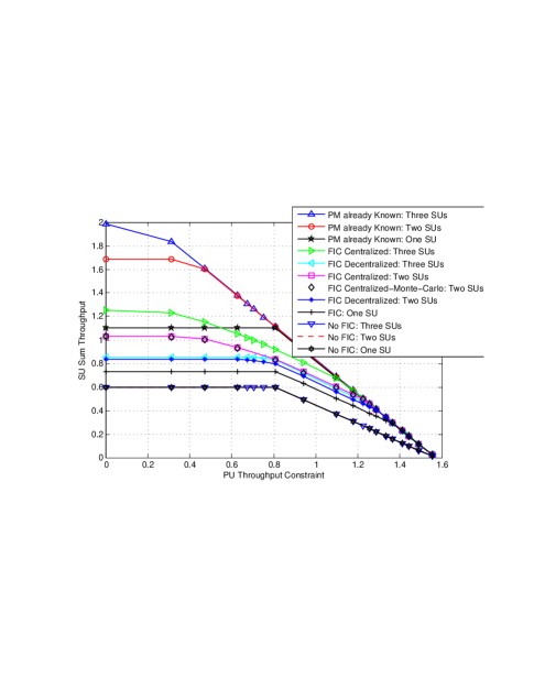
Figure 3: Average sum throughput of SUs with respect to PU throughput constraint $(1-\epsilon_{PU})T_{pu}^{I}$. $\bar{\gamma}_{ps_{n}}=5$, $\bar{\gamma}_{s_{n}p}=2$, $\bar{\gamma}_{pp}=10$, $\bar{\gamma}_{s_{n}s_{n}}=5$ and $\bar{\gamma}_{s_{n}s_{m}}=3$, $n,m\in\{1,...,N\}$, $n\neq m$.

The average sum throughput of SUs as a function of $\bar{\gamma}_{s_{1}p}$ is depicted in Fig. 4, where $\bar{\gamma}_{s_{2}p}=2$. As observed, the SU sum throughput decreases as $\bar{\gamma}_{s_{1}p}$ increases. This is because $\bar{\gamma}_{s_{2}p}=2$ and hence, the PU throughput degradation constraint is always active for the two SUs. A similar plot for the case $\bar{\gamma}_{s_{2}p}=\bar{\gamma}_{s_{1}p}$ is depicted in Fig. 5. As observed, for $\bar{\gamma}_{s_{1}p}<0.5$, $\bar{\gamma}_{s_{1}p}<0.25$ and $\bar{\gamma}_{s_{1}p}<0.45$ respectively in the CRN with one SU, centralized and decentralized cases, we have a different result. In fact, because the interference power of SUs has little effect on the PU receiver, initially the PU throughput degradation constraint is not active and therefore $SU_{tx1}$ and $SU_{tx2}$ may utilize their powers to maximize their own throughput. Note that the action obtained for the SUs when $\bar{\gamma}_{s_{1}p}=0.25$ can not be used for $\bar{\gamma}_{s_{1}p}<0.25$. In fact, notice that as $\bar{\gamma}_{s_{1}p}$ and $\bar{\gamma}_{s_{2}p}$ increase, the activity of the SUs causes more interference at the PU receiver and leads to more ARQ retransmissions. In turn, this will make more IC opportunities available at the SU receivers, thereby increasing the SU sum throughput. On the other hand, since for PM already Known and “No FIC” the SUs assume that the PU messages are already known or they do not apply IC, respectively, there is no benefit in augmenting the ARQ retransmissions and therefore the performance is constant for small $\bar{\gamma}_{s_{1}p}$ and $\bar{\gamma}_{s_{2}p}$, until the constraint becomes active for $\bar{\gamma}_{s_{1}p}>0.5$, $\bar{\gamma}_{s_{1}p}=\bar{\gamma}_{s_{2}p}>0.25$ and $\bar{\gamma}_{s_{1}p}=\bar{\gamma}_{s_{2}p}>0.45$, respectively in the CRN with one SU, centralized and decentralized cases; therefore, above those values, the SU sum throughput decreases. As expected, in the cognitive radio with two symmetric SUs and centralized scenario, the PU throughput degradation constraint becomes active sooner than in the cognitive radio with one SU, when increasing the SNR of the channels from the SU transmitters to the PU receiver. A similar observation can be made when $\bar{\gamma}_{ps_{1}}=\bar{\gamma}_{ps_{2}}=2$ as depicted in Fig. 6. Our results, not shown here, confirm the same observation for $N=3$ when compared with $N=2$. It is noteworthy that because $\bar{\gamma}_{ps_{1}}=\bar{\gamma}_{ps_{2}}=2$ are neither strong enough to be successfully decoded, nor so weak as to be considered as small noise at the SU receivers, the SU sum throughput provided by the centralized case suffers a higher performance loss with respect to the upper bound compared with that in Fig. 5. This observation is clearly seen also in the next two figures, as discussed later.

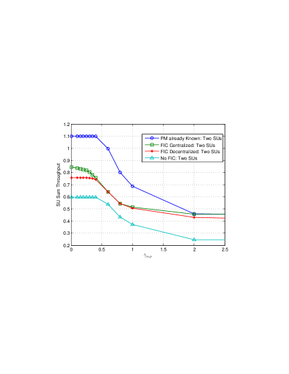
Figure 4: Average sum throughput of SUs with respect to $\bar{\gamma}_{s_{1}p}$. $\bar{\gamma}_{ps_{1}}=\bar{\gamma}_{ps_{2}}=5$, $\bar{\gamma}_{s_{2}p}=2$, $\bar{\gamma}_{pp}=10$, $\bar{\gamma}_{s_{1}s_{1}}=\bar{\gamma}_{s_{2}s_{2}}=5$, $\bar{\gamma}_{s_{1}s_{2}}=\bar{\gamma}_{s_{2}s_{1}}=3$ and $\epsilon_{PU}=0.2$.

Figure 5: Average sum throughput of SUs with respect to $\bar{\gamma}_{s_{1}p}=\bar{\gamma}_{s_{2}p}$. $\bar{\gamma}_{ps_{1}}=\bar{\gamma}_{ps_{2}}=5$, $\bar{\gamma}_{pp}=10$, $\bar{\gamma}_{s_{1}s_{1}}=\bar{\gamma}_{s_{2}s_{2}}=5$, $\bar{\gamma}_{s_{1}s_{2}}=\bar{\gamma}_{s_{2}s_{1}}=3$ and $\epsilon_{PU}=0.2$.

Figure 6: Average sum throughput of SUs with respect to $\bar{\gamma}_{s_{1}p}=\bar{\gamma}_{s_{2}p}$. $\bar{\gamma}_{ps_{1}}=\bar{\gamma}_{ps_{2}}=2$, $\bar{\gamma}_{pp}=10$, $\bar{\gamma}_{s_{1}s_{1}}=\bar{\gamma}_{s_{2}s_{2}}=5$, $\bar{\gamma}_{s_{1}s_{2}}=\bar{\gamma}_{s_{2}s_{1}}=3$ and $\epsilon_{PU}=0.2$.

Figs. 7 and 8 show the average SU sum throughput with respect to $\bar{\gamma}_{ps_{1}}$ for $\bar{\gamma}_{ps_{2}}=5$ and $\bar{\gamma}_{ps_{2}}=\bar{\gamma}_{ps_{1}}$, respectively. Note that $R^{*}_{s_{1},a,\Phi=(U,\theta)}$ and $R^{*}_{s_{2},a,\Phi=(\theta,U)}$ respectively depend on $\bar{\gamma}_{ps_{1}}$ and $\bar{\gamma}_{ps_{2}}$. As expected, $\bar{\gamma}_{ps_{1}}$ does not have any influence on the “PM already Known” scheme. This is because in this scheme the PU message is previously known and can always be canceled by the SU receiver in future retransmissions. It is observed that for large enough values of $\bar{\gamma}_{ps_{1}}$, the upper bound is achievable by the FIC scheme in the centralized scenario. In fact, the SU receiver can successfully decode the PU message, remove the interference and decode its corresponding message. Note that the upper bound is computed in the centralized scenario. The sum throughput is minimized at $\bar{\gamma}_{ps_{1}}=2$ in the CRN with one SU, centralized and decentralized cases, where the PU message is neither strong enough to be successfully decoded, nor weak to be considered as negligible. It is also evident that the FIC scheme in Fig. 7 converges to the upper bound faster than in Fig. 8. The reason is that $\bar{\gamma}_{sp_{1}}$ and $\bar{\gamma}_{sp_{2}}$ increase simultaneously in Fig. 8, whereas the value of $\bar{\gamma}_{sp_{2}}$ is considered to be equal to zero in Fig. 7, resulting in no interference to the PU receiver. It is also observed from Fig. 8 that a cognitive radio with two symmetric SUs converges to the upper bound faster than the network with one SU for large enough SNR of the channels from the PU transmitter to SU receivers. This is because of the use of the FIC scheme at the SU receivers. A similar behavior has been observed in a CRN with $N=3$.

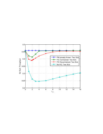
Figure 7: Average sum throughput of SUs with respect to $\bar{\gamma}_{ps_{1}}$. $\bar{\gamma}_{ps_{2}}=5$, $\bar{\gamma}_{s_{1}p}=\bar{\gamma}_{s_{2}p}=2$, $\bar{\gamma}_{pp}=10$, $\bar{\gamma}_{s_{1}s_{1}}=\bar{\gamma}_{s_{2}s_{2}}=5$, $\bar{\gamma}_{s_{1}s_{2}}=\bar{\gamma}_{s_{2}s_{1}}=3$ and $\epsilon_{PU}=0.2$.

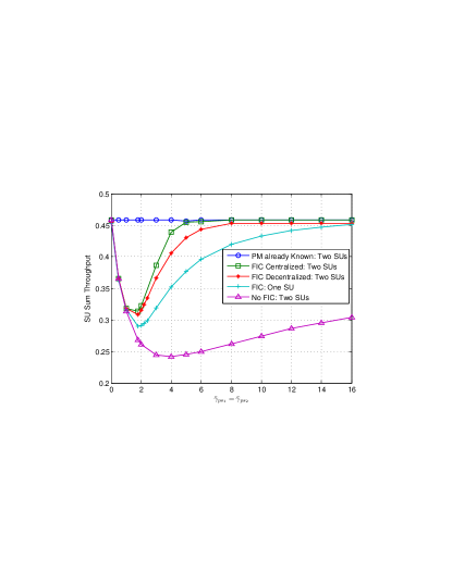
Figure 8: Average sum throughput of SUs with respect to $\bar{\gamma}_{ps_{1}}=\bar{\gamma}_{ps_{2}}$. $\bar{\gamma}_{s_{1}p}=\bar{\gamma}_{s_{2}p}=2$, $\bar{\gamma}_{pp}=10$, $\bar{\gamma}_{s_{1}s_{1}}=\bar{\gamma}_{s_{2}s_{2}}=5$, $\bar{\gamma}_{s_{1}s_{2}}=\bar{\gamma}_{s_{2}s_{1}}=3$ and $\epsilon_{PU}=0.2$.

VII Extension to Decentralized Access Policy Design with Partially State Information

In this section, we discuss a possible model for the decentralized scenario when the PU message knowledge state is known partially for the SUs in addition to the action being selected by the SU independently of the other SUs. In Section V, the PU message knowledge state of each SU was assumed to be also known to the other SUs, which makes the whole state of the system known to all SUs. Now we assume that each user can only observe its own PU message knowledge state. When there is an uncertainty about the state of the system, the problem is called “Distributed Partial State Information MDP” (DEC-PSI-MDP) which is a type of “Partially Observable MDP” (DEC-POMDP). For a literature review on the decentralized control of DEC-POMDP, the reader is referred to [23]. In this model, the shared objective function is used (here the SU Sum throughput) and the action is selected based on the partial state observation at each SU. Because each secondary user is unaware of the belief states of the other users, it is impossible for each user to properly estimate the state of the system. Thus, a DEC-POMDP can not be formulated as an MDP by introducing beliefs. It can be shown that DEC-POMDP is nondeterministic exponential (NEXP) complete even for two users [24] and, hence, only approximate solutions can be applied [22]. Consideration of this type of system is left as future work.

VIII Conclusion

In this paper, an optimal access policy for an arbitrary number of cognitive secondary users was proposed, under a constraint on the interference from the secondary users to the primary receiver. Leveraging the inherent redundancy of the ARQ retransmissions implemented by the PU, each SU receiver can cancel a successfully decoded PU message in the following ARQ retransmissions, thereby improving its own throughput. Both centralized and decentralized scenarios were considered. In the first scenario, there is a centralized unit which controls the access to the channel of all SUs, to maximize the average sum throughput of the SUs under the average PU throughput degradation constraint. In the decentralized scenario, there exists no central unit and therefore each SU makes an access decision independently of the other SUs, while the state of the system is still assumed to be known to all secondary users. In the centralized case, an upper bound was formulated and a close form solution was provided. Our studies confirm that the centralized and decentralized scenarios may be modeled as CMDP and MMDP and therefore solved by linear programming. At the end, extension of the problem to CRN with partial state information was discussed.

Appendix A Proof of Proposition 1

Define:

$$d_{i}=Dec2Bin_{N}(i).({T}_{s_{1},i,(K,...,K)},...,{T}_{s_{N},i,(K,...,K)})\;\;\;i\in\{1,...,2^{N}-1\},$$ (53)

where ${T}_{s_{n},i,(K,...,K)}$, $n\in\{1,...,N\}$ is given in (8). A list of all situations is given here in detail for $N=2$, and can be extended to an arbitrary $N$.

1. $\lambda_{1}=0$ and $\lambda_{2}=0$. From (22), it is necessary to have

   $$d_{i}=0\;\;\;i\in\{1,2,3\}$$ (54)

   Hence, this case is not acceptable.

2. $\mu_{i}=0,\;i\in\{1,2,3\}$. This case gives an SU sum throughput equal to zero and hence does not provide the optimum solution.

3. $\lambda_{1}>0$, $\lambda_{2}=0$, $\mu_{i}>0,\mu_{j}=0,\mu_{k}=0$, $(i,j,k)\in\{(1,2,3),(2,1,3),(3,1,2)\}$. It is observed from condition (22) that $\frac{\partial L}{\partial\mu_{i}}=0$, $\frac{\partial L}{\partial\mu_{j}}\leq 0$ and $\frac{\partial L}{\partial\mu_{k}}\leq 0$. This occurs if

   $$\frac{d_{j}}{{\rho_{p,j}-\rho_{p,0}}}\leq\frac{d_{i}}{{\rho_{p,i}-\rho_{p,0}}}$$ (55)

   $$\frac{d_{k}}{{\rho_{p,k}-\rho_{p,0}}}\leq\frac{d_{i}}{{\rho_{p,i}-\rho_{p,0}}}$$ (56)

   Noting (23) and (24), we have $\mu_{i}({\rho_{p,i}-\rho_{p,0}})=\epsilon_{\omega}$ and $\mu_{i}\leq 1$; or equivalently

   $$\mu_{i}=\frac{\epsilon_{\omega}}{\rho_{p,i}-\rho_{p,0}}\leq 1.$$ (57)

   Thus, the resulting maximum SU sum throughput is equal to $\frac{\epsilon_{\omega}}{\rho_{p,i}-\rho_{p,0}}{d_{i}}$.

4. $\lambda_{1}=0$, $\lambda_{2}>0$, $\mu_{i}>0,\mu_{j}=0,\mu_{k}=0$, $(i,j,k)\in\{(1,2,3),(2,1,3),(3,1,2)\}$. It is observed from condition (22) that $\frac{\partial L}{\partial\mu_{i}}=0$, $\frac{\partial L}{\partial\mu_{j}}\leq 0$ and $\frac{\partial L}{\partial\mu_{k}}\leq 0$. This occurs if

   $$d_{k}\leq d_{i}$$ (58)

   $$d_{j}\leq d_{i}.$$ (59)

   Noting (23) and (24), we have $\mu_{i}({\rho_{p,i}-\rho_{p,0}})\leq\epsilon_{\omega}$ and $\mu_{i}=1$; or equivalently

   $$\mu_{i}=1\leq\frac{\epsilon_{\omega}}{\rho_{p,i}-\rho_{p,0}}.$$ (60)

   Thus, the resulting maximum SU sum throughput is equal to $d_{i}$.

5. $\lambda_{1}>0$, $\lambda_{2}>0$, $\mu_{i}>0,\mu_{j}=0,\mu_{k}=0$, $(i,j,k)\in\{(1,2,3),(2,1,3),(3,1,2)\}$. It is observed from condition (22) that $\frac{\partial L}{\partial\mu_{i}}=0$, $\frac{\partial L}{\partial\mu_{j}}\leq 0$ and $\frac{\partial L}{\partial\mu_{k}}\leq 0$. This occurs if

   $$d_{k}\geq d_{i}\;\;\;\mathrm{if}\;{{\rho_{p,k}-\rho_{p,0}}\geq{\rho_{p,i}-\rho_{p,0}}}$$ (61)

   $$d_{k}<d_{i}\;\;\;\mathrm{if}\;{{\rho_{p,k}-\rho_{p,0}}<{\rho_{p,i}-\rho_{p,0}}}$$ (62)

   $$d_{j}\geq d_{i}\;\;\;\mathrm{if}\;{{\rho_{p,j}-\rho_{p,0}}\geq{\rho_{p,i}-\rho_{p,0}}}$$ (63)

   $$d_{j}<d_{i}\;\;\;\mathrm{if}\;{{\rho_{p,j}-\rho_{p,0}}<{\rho_{p,i}-\rho_{p,0}}}.$$ (64)

   Noting (23) and (24), we have

   $$\mu_{i}=1=\frac{\epsilon_{\omega}}{\rho_{p,i}-\rho_{p,0}}.$$ (65)

   Thus, the resulting maximum SU sum throughput is equal to $d_{i}$.

6. $\lambda_{1}>0$, $\lambda_{2}=0$, $\mu_{1}>0,\mu_{2}>0,\mu_{3}>0$. It is observed from condition (22) that $\frac{\partial L}{\partial\mu_{1}}=\frac{\partial L}{\partial\mu_{2}}=\frac{\partial L}{\partial\mu_{3}}=0$. This occurs if

   $$\frac{d_{1}}{{\rho_{p,1}-\rho_{p,0}}}=\frac{d_{2}}{{\rho_{p,2}-\rho_{p,0}}}=\frac{d_{3}}{{\rho_{p,3}-\rho_{p,0}}}.$$ (66)

   Noting (23) and (24), $\mu_{1}({\rho_{p,1}-\rho_{p,0}})+\mu_{2}({\rho_{p,2}-\rho_{p,0}})+\mu_{3}({\rho_{p,3}-\rho_{p,0}})=\epsilon_{\omega}$ and $\mu_{1}+\mu_{2}+\mu_{3}\leq 1$. These two conditions impose that

   $$\epsilon_{\omega}\leq{\rho_{p,3}-\rho_{p,0}}.$$ (67)

   Thus, the resulting maximum SU sum throughput is equal to $\frac{\epsilon_{\omega}{d_{1}}}{{\rho_{p,1}-\rho_{p,0}}}$.

7. $\lambda_{1}=0$, $\lambda_{2}>0$, $\mu_{1}>0,\mu_{2}>0,\mu_{3}>0$. It is observed from condition (22) that $\frac{\partial L}{\partial\mu_{1}}=\frac{\partial L}{\partial\mu_{2}}=\frac{\partial L}{\partial\mu_{3}}=0$. This occurs if

   $$d_{1}=d_{2}=d_{3}.$$ (68)

   Noting (23) and (24), $\mu_{1}({\rho_{p,1}-\rho_{p,0}})+\mu_{2}({\rho_{p,2}-\rho_{p,0}})+\mu_{3}({\rho_{p,3}-\rho_{p,0}})\leq\epsilon_{\omega}$ and $\mu_{1}+\mu_{2}+\mu_{3}=1$. The conditions impose that

   $$\operatorname{min}{(\rho_{p,1}-\rho_{p,0},\rho_{p,2}-\rho_{p,0})}\leq\epsilon_{\omega}.$$ (69)

   Thus, the resulting maximum SU sum throughput is equal to $d_{1}$.

8. $\lambda_{1}>0$, $\lambda_{2}>0$, $\mu_{1}>0,\mu_{2}>0,\mu_{3}>0$. It is observed from condition (22) that $\frac{\partial L}{\partial\mu_{1}}=\frac{\partial L}{\partial\mu_{2}}=\frac{\partial L}{\partial\mu_{3}}=0$. This occurs if

   $$d_{i}\leq d_{3}\;\;\;i\in\{1,2\}$$ (70)

   $$d_{1}\geq d_{2}\;\;\;\mathrm{if}\;{{\rho_{p,1}-\rho_{p,0}}\geq{\rho_{p,2}-\rho_{p,0}}}$$ (71)

   $$d_{1}<d_{2}\;\;\;\mathrm{if}\;{{\rho_{p,1}-\rho_{p,0}}<{\rho_{p,2}-\rho_{p,0}}}$$ (72)

   $$\frac{d_{3}}{\rho_{p,3}-\rho_{p,0}}<\operatorname{min}\{\frac{d_{1}}{\rho_{p,1}-\rho_{p,0}},\frac{d_{2}}{\rho_{p,2}-\rho_{p,0}}\}$$ (73)

   $$\frac{d_{1}}{\rho_{p,1}-\rho_{p,0}}\geq\frac{d_{2}}{\rho_{p,2}-\rho_{p,0}}\;\;\;\mathrm{if}\;{{\rho_{p,1}-\rho_{p,0}}\leq{\rho_{p,2}-\rho_{p,0}}}$$ (74)

   $$\frac{d_{1}}{\rho_{p,1}-\rho_{p,0}}<\frac{d_{2}}{\rho_{p,2}-\rho_{p,0}}\;\;\;\mathrm{if}\;{{\rho_{p,1}-\rho_{p,0}}>{\rho_{p,2}-\rho_{p,0}}}$$ (75)

   Noting (23) and (24), $\mu_{1}({\rho_{p,1}-\rho_{p,0}})+\mu_{2}({\rho_{p,2}-\rho_{p,0}})+\mu_{3}({\rho_{p,3}-\rho_{p,0}})=\epsilon_{\omega}$ and $\mu_{1}+\mu_{2}+\mu_{3}=1$. The conditions impose that

   $$\operatorname{min}{(\rho_{p,1}-\rho_{p,0},\rho_{p,2}-\rho_{p,0})}\leq\epsilon_{\omega}\leq\operatorname{max}{(\rho_{p,1}-\rho_{p,0},\rho_{p,2}-\rho_{p,0})}$$ (76)

   $$\epsilon_{\omega}\leq{\rho_{p,3}-\rho_{p,0}}.$$ (77)

   Thus, the resulting maximum SU sum throughput is equal or lower than $\epsilon_{\omega}\operatorname{max}{(\frac{d_{1}}{\rho_{p,1}-\rho_{p,0}},\frac{d_{2}}{\rho_{p,2}-\rho_{p,0}})}$ and the equality is achieved when $\frac{d_{1}}{\rho_{p,1}-\rho_{p,0}}=\frac{d_{2}}{\rho_{p,2}-\rho_{p,0}}$.

9. $\lambda_{1}>0$, $\lambda_{2}=0$, $\mu_{i}=0,\mu_{j}>0,\mu_{k}>0$, $(i,j,k)\in\{(1,2,3),(2,1,3),(3,1,2)\}$. It is observed from condition (22) that $\frac{\partial L}{\partial\mu_{i}}\leq 0$, $\frac{\partial L}{\partial\mu_{j}}=0$ and $\frac{\partial L}{\partial\mu_{k}}=0$. This occurs if

   $$\frac{d_{i}}{{\rho_{p,i}-\rho_{p,0}}}\leq\frac{d_{j}}{\rho_{p,j}-\rho_{p,0}}=\frac{d_{k}}{\rho_{p,k}-\rho_{p,0}}.$$ (78)

   Noting (23) and (24), $\mu_{j}({\rho_{p,j}-\rho_{p,0}})+\mu_{k}({\rho_{p,k}-\rho_{p,0}})=\epsilon_{\omega}$ and $\mu_{j}+\mu_{k}\leq 1$. The conditions impose that

   $$\epsilon_{\omega}\leq\operatorname{max}{(\rho_{p,j}-\rho_{p,0},\rho_{p,k}-\rho_{p,0})}.$$ (79)

   and the resulting maximum SU sum throughput is equal to $\frac{\epsilon_{\omega}{d_{j}}}{{\rho_{p,j}-\rho_{p,0}}}$.

10. $\lambda_{1}=0$, $\lambda_{2}>0$, $\mu_{i}=0,\mu_{j}>0,\mu_{k}>0$, $(i,j,k)\in\{(1,2,3),(2,1,3),(3,1,2)\}$. It is observed from condition (22) that $\frac{\partial L}{\partial\mu_{i}}\leq 0$, $\frac{\partial L}{\partial\mu_{j}}=0$ and $\frac{\partial L}{\partial\mu_{k}}=0$. This occurs if

    $$d_{i}\leq{d_{j}}=d_{k}.$$ (80)

    Noting (23) and (24), $\mu_{j}({\rho_{p,j}-\rho_{p,0}})+\mu_{k}({\rho_{p,k}-\rho_{p,0}})\leq\epsilon_{\omega}$ and $\mu_{j}+\mu_{k}=1$. The conditions impose that

    $$\operatorname{min}{(\rho_{p,j}-\rho_{p,0},\rho_{p,k}-\rho_{p,0})}\leq\epsilon_{\omega}.$$ (81)

    The resulting maximum SU sum throughput is equal to $d_{j}$.

11. $\lambda_{1}>0$, $\lambda_{2}>0$, $\mu_{i}=0,\mu_{j}>0,\mu_{k}>0$, $(i,j,k)\in\{(1,2,3),(2,1,3),(3,1,2)\}$. It is observed from condition (22) that $\frac{\partial L}{\partial\mu_{i}}\leq 0$, $\frac{\partial L}{\partial\mu_{j}}=0$ and $\frac{\partial L}{\partial\mu_{k}}=0$. This occurs if

    $$d_{j}\geq d_{k}\;\;\;\mathrm{if}\;{{\rho_{p,j}-\rho_{p,0}}\geq{\rho_{p,k}-\rho_{p,0}}}$$ (82)

    $$d_{j}<d_{k}\;\;\;\mathrm{if}\;{{\rho_{p,j}-\rho_{p,0}}<{\rho_{p,k}-\rho_{p,0}}}$$ (83)

    $$\frac{d_{j}}{\rho_{p,j}-\rho_{p,0}}\geq\frac{d_{k}}{\rho_{p,k}-\rho_{p,0}}\;\;\;\mathrm{if}\;{{\rho_{p,j}-\rho_{p,0}}\leq{\rho_{p,k}-\rho_{p,0}}}$$ (84)

    $$\frac{d_{j}}{\rho_{p,j}-\rho_{p,0}}<\frac{d_{k}}{\rho_{p,k}-\rho_{p,0}}\;\;\;\mathrm{if}\;{{\rho_{p,j}-\rho_{p,0}}>{\rho_{p,k}-\rho_{p,0}}}$$ (85)

    $$d_{i}\geq d_{j}\;\;\;\mathrm{if}\;{{\rho_{p,i}-\rho_{p,0}}\geq{\rho_{p,j}-\rho_{p,0}}}$$ (86)

    $$d_{i}<d_{j}\;\;\;\mathrm{if}\;{{\rho_{p,i}-\rho_{p,0}}<{\rho_{p,j}-\rho_{p,0}}}$$ (87)

    $$d_{i}\geq d_{k}\;\;\;\mathrm{if}\;{{\rho_{p,i}-\rho_{p,0}}\geq{\rho_{p,k}-\rho_{p,0}}}$$ (88)

    $$d_{i}<d_{k}\;\;\;\mathrm{if}\;{{\rho_{p,i}-\rho_{p,0}}<{\rho_{p,k}-\rho_{p,0}}}$$ (89)

    Noting (23) and (24), $\mu_{j}({\rho_{p,j}-\rho_{p,0}})+\mu_{k}({\rho_{p,k}-\rho_{p,0}})=\epsilon_{\omega}$ and $\mu_{j}+\mu_{k}=1$. The conditions impose that

    $$\operatorname{min}{(\rho_{p,j}-\rho_{p,0},\rho_{p,k}-\rho_{p,0})}\leq\epsilon_{\omega}\leq\operatorname{max}{(\rho_{p,j}-\rho_{p,0},\rho_{p,k}-\rho_{p,0})}.$$ (90)

    The resulting maximum SU sum throughput is equal or lower than $\epsilon_{\omega}\operatorname{max}{(\frac{d_{j}}{\rho_{p,j}-\rho_{p,0}},\frac{d_{k}}{\rho_{p,k}-\rho_{p,0}})}$ and the equality is achieved when $\frac{d_{j}}{\rho_{p,j}-\rho_{p,0}}=\frac{d_{k}}{\rho_{p,k}-\rho_{p,0}}$.

Noting items 1 to 11, it is observed that items $3$, $4$, $6$, $7$, $9$, $10$ provide optimum solutions and hence, the optimum access policy and SU Sum throughput can be summarized in (19) and (20) respectively. Thus, the proof is complete.

References

• [1] R. Joda and M. Zorzi, “Centralized access policy design for two cognitive secondary users under a primary ARQ process,” Proc. IEEE Conf. Commun. Workshop on Cooperative and Cognitive Mobile Networks, 2014.
• [2] J. Mitola and G. Maguire, “Cognitive radio: Making software radios more personal,” IEEE Personal Commun. Mag., vol. 24, pp. 13–18, May 1999.
• [3] J. M. Peha, “Approaches to spectrum sharing,” IEEE Commun. Mag., vol. 43, pp. 10–12, Feb. 2005.
• [4] J. M. Peha, “Sharing spectrum through spectrum policy reform and cognitive radio,” Proc. IEEE, vol. 97, pp. 708–719, Apr. 2009.
• [5] Q. Zhao and B. M. Sadler, “A survey of dynamic spectrum access: Signal processing, networking, and regulatory policy,” IEEE Signal Process. Mag., vol. 24, pp. 79–89, May 2007.
• [6] K. G. Shin, H. Kim, A. W. Min, and A. Kumar, “Cognitive radios for dynamic spectrum access: From concept to reality,” IEEE Trans. Wireless Commun., vol. 17, pp. 64–74, Dec. 2010.
• [7] I. Akyildiz, W. Y. Lee, M. Vuran, and S. Mohanty, “A survey on spectrum management in cognitive radio networks,” IEEE Commun. Mag., vol. 46, pp. 40–48, Apr 2008.
• [8] M. Levorato, U. Mitra, and M. Zorzi, “Cognitive interference management in retransmission-based wireless networks,” IEEE Trans. Inform. Theory, vol. 58, pp. 3023–3046, May 2012.
• [9] N. Michelusi, P. Popovski, O. Simeone, M. Levorato, and M. Zorzi, “Cognitive access policies under a primary ARQ process via forward-backward interference cancellation,” IEEE J. Sel. Areas Commun., vol. 31, pp. 2374–2486, Nov. 2013.
• [10] N. Michelusi, P. Popovski, and M. Zorzi, “Cognitive access policies under a primary ARQ process via chain decoding,” ITA Workshop, 2013.
• [11] R. Tannious and A. Nosratinia, “Cognitive radio protocols based on exploiting hybrid ARQ retransmissions,” IEEE Trans. Wireless Commun., vol. 9, pp. 2833–2841, Sept. 2010.
• [12] R. Tajan, C. Poulliat, and I. Fijalkow, “Opportunistic secondary spectrum sharing protocols for primary implementing an IR type Hybrid-ARQ protocol,” Proc. IEEE ICASSP, pp. 3233–3236, 2012.
• [13] J. C. F. Li, W. Zhang, A. Nosratinia, and J. Yuan, “SHARP: Spectrum harvesting with ARQ retransmission and probing in cognitive radio,” IEEE Trans. Commun., vol. 61, pp. 951–960, Mar. 2013.
• [14] R. Tajan, C. Poulliat, and I. Fijalkow, “Interference management for cognitive radio systems exploiting primary IR-HARQ: a constrained Markov decision process approach,” Proc. IEEE Asilomar Conf. Signals, Systems and Computers, pp. 1818–1822, Nov. 2012.
• [15] R. Joda and M. Zorzi, “Centralized power allocation policy design for cognitive secondary users under a primary Type-II HARQ process,” IEEE Conf. Computing, Networking and Communications (ICNC), Feb. 2015.
• [16] C. Boutilier, “Planning, learning and coordination in multiagent decision processes,” Proc. of the Conference on Theoretical Aspects of Rationality and Knowledge, pp. 195–210, 1996.
• [17] K. W. Ross, “Randomized and pastdependent policies for Markov decision processes with multiple constraints,” Operations Research, vol. 37, no. 3, pp. 474–477, 1989.
• [18] E. Altman, “The linear program approach in multi-chain Markov decision processes revisited,” Mathematical Methods of Operations Research, vol. 42, pp. 169–188, 1995.
• [19] R. Joda and M. Zorzi, “Access policy design for two cognitive secondary users under a primary ARQ process,” [Online.] Available: http://arxiv.org/abs/1410.4155.
• [20] E. Altman, “Constrained Markov decision processes,” CRC Press, vol. 7, 1999.
• [21] B. S. I. Chad‘es and F. Charpillet, “A heuristic approach for solving decentralized-POMDP: Assessment on the pursuit problem,” Proc. of the Sixteenth ACM Symposium on Applied Computing, 2002.
• [22] R. Nair, M. Tambe, M. Yokoo, D. V. Pynadath, and S. Marsella, “Taming decentralized POMDPs: Towards efficient policy computation for multiagent settings,” Proc. of the 18th Int. Joint Conf. on Artificial Intelligence, pp. 705–711, 2003.
• [23] C. Amato, G. Chowdhary, A. Geramifard, N. K. Ure, and M. J. Kochenderfer, “Decentralized control of partially observable Markov decision processes,” IEEE Conference on Decision and Control, pp. 2398–2405, 2013.
• [24] D. S. Bernstein, R. Givan, N. Immerman, and S. Zilberstein, “The complexity of decentralized control of Markov decision processes,” Mathematics of Operations Research, vol. 27, no. 4, pp. 819–840, 2002.