Robust Topological Feature Extraction for Mapping of Environments using Bio-Inspired Sensor Networks

Abstract

In this paper, we exploit minimal sensing information gathered from biologically inspired sensor networks to perform exploration and mapping in an unknown environment. A probabilistic motion model of mobile sensing nodes, inspired by motion characteristics of cockroaches, is utilized to extract weak encounter information in order to build a topological representation of the environment. Neighbor to neighbor interactions among the nodes are exploited to build point clouds representing spatial features of the manifold characterizing the environment based on the sampled data. To extract dominant features from sampled data, topological data analysis is used to produce persistence intervals for features, to be used for topological mapping. In order to improve robustness characteristics of the sampled data with respect to outliers, density based subsampling algorithms are employed. Moreover, a robust scale-invariant classification algorithm for persistence diagrams is proposed to provide a quantitative representation of desired features in the data. Furthermore, various strategies for defining encounter metrics with different degrees of information regarding agents’ motion are suggested to enhance the precision of the estimation and classification performance of the topological method.

Introduction

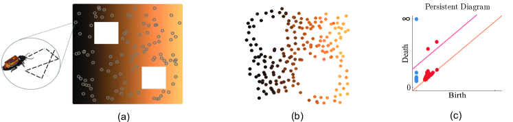
Figure 1: Topologcal Mapping: (a) a physical environment with mobile sensing nodes moving inspired by cockroaches, (b) an esimated point cloud from coordinate free information, (c) the corresponding persistence diagram highlighting the features in dim 0 (blue dots) the features in dim 1 (red dots); significant features can be distinguished from noise using an appropriate threshhold.

Sensor networks with their broad application in mapping and navigation [1], habitat monitoring [2], exploration, and search and rescue [3], have attracted a lot of attention in recent decades. Mobile sensor networks offer the flexibility to adapt with dynamic environments. As an example, swarm robotic systems, where mobility models of agents are inspired by biological entities, and each agent is equipped with some type of sensing, are considered as mobile sensor networks which can perform distributed sensing and estimation tasks. Emergent behavior in animals such as formation[4], coverage[5], and aggregation[6] have inspired scientists to develop behavioral-based distributed systems.

In some applications, however, the amount of information that could be sensed or transferred by the agents is limited. This motivates the design of distributed systems composed of simple agents with minimal sensing requirements[7]. Consider for example a disaster zone response scenario, where we aim to perform exploration and mapping of an unstructured and unknown environment using a mobile sensor network. One may choose to make use of a swarm of biologically inspired agents with minimal sensing capabilities to perform the task. However, under such rough conditions of the terrain, localization information provided by the agents could be very weak and contains a high amount of uncertainty. Hence, traditional localization and mapping algorithms such as SLAM[8] would fail to perform effectively.

Methods from computational topology, on the other hand, can provide tools to extract topological features from data sets without requiring coordinate information. This makes them more suitable for scenarios in which weak or no localization is provided. Topological data analysis (TDA), introduced in [9], has been a new field of study which employs tools from persistent homology theory [10] to obtain a qualitative description of the topological attributes and visualization of data sets sampled from high dimensional point clouds. The point cloud can be thought of as finite samples taken from a density map which may include noise. TDA represents the prominence of features in the point cloud in terms of a compact representation of the multi-scale topological structure called persistence diagrams[11]. It reduces the dimensions of data by construction of a filtration of combinatorial objects, which can represent geometrical and topological features of the data set at specific scales.

Topological frameworks have been used for characterization of coverage and hole detection in stationary sensor networks by using only proximity information of the nodes within a neighborhood[12, 13]. However, these studies mostly focused on networks with static nodes. Moreover, they are mainly concerned about the coverage holes in the sensing domain of the network rather than the topology of the physical environment itself. Adding mobility to the nodes in the network makes the problem more challenging. One way to reduce such complexity is to look for patterns created by tracing the encounters of the nodes instead of investigating the mobility data itself. Walker [14] employed persistent homology to compute topological invariants from encounter data of the mobile nodes in Mobile Ad-Hoc networks in order to infer global information regarding the topology of a physical environment, but the nodes are assumed to follow a simple mobility model on a graph.

Contribution: In this paper, we aim to construct topological maps of unknown environments using bio-inspired mobile sensor networks under the constraint of limited sensing information. In particular, we consider agents whose movement model is described by the motion model of cockroaches, which are experts to survive in harsh environments. We develop algorithms that do not depend on any type of traditional localization schemes. Instead, we consider estimation of a topological model for the environment based on limited information retrieved from the agents including their own status, and their encounters with other agents in their proximity. We propose various types of metrics for the construction of point clouds based on coordinate-free information that estimate topological features of the environment. Moreover, density based subsampling methods are used to deal with outliers produced as a result of uncertainty in the estimated point clouds. Computational topology algorithms are used to extract dominance of these features in terms of persistence intervals. However, such intervals provide qualitative representation about low dimensional structures in the point cloud. Hence, methods from machine learning and statistical data analysis recently have been integrated with persistence analysis in order to make inference and interpretation out of such intervals [15, 16]. In this study, we develop a density based classification algorithm to extract features from persistence intervals quantitatively in a robust manner to be used in the construction of the topological map.

The remainder of the paper is organized as follows: A concise background on TDA is presented in section 2. Bio-inspired mobility model as well as sensing model for the nodes are described in section 3, followed by a general overview of the proposed mapping framework. Section 4 discusses the different metrics employed for construction of point clouds. Subsampling techniques are described in section 5, and classification algorithm for dominant features is proposed in section 6. Finally, conclusion and future extensions of the presented work are discussed in Section 7.

Background on TDA

A brief introduction of some of the basic concepts in computational topology is presented here. A comprehensive review of the topic can be found in [11].

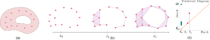
Figure 2: Topological persistence: (a) An example of a topological space $M$ with a sampled point cloud $X$, (b) a filtration of complexes over $X$, (c) the corresponding persistence diagram ( dgm${}_{0}(X)$ in dark cyan and dgm${}_{1}(X)$ in red)

One of the well-known techniques widely used in topological data analysis is persistent homology, which deals with the way that objects are connected. Topological structures of a space $M$ are summarized as a compact representation in the form of so-called Betti numbers, which are ranks of topological invariants, called homology groups. The $n$-th Betti number, $\beta_{n}$ measures the number of $n$-dimensional cycles in the space (e.g. $\beta_{0}$ is the number of connected components and $\beta_{1}$ is the number of holes in the complex). The space $M$ usually is not directly accessible but a sampled version of it, ${X,}$ can be used for computations. This sample is represented as a point cloud, a finite set of points equipped with a metric, which can be defined by pairwise distances between the points.

A standard method to analyze the topological structure of a point cloud is to map it into combinatorial objects called simplicial complexes. One way to build these complexes is to select a scale $\epsilon$, place balls of radius $\epsilon$ on each vertex, and construct simplices based on their pairwise distance relative to $\epsilon$. A computationally efficient complex, called Vietoris-Rips complex [17] consists of simplices for which the distances between each pair of its vertices are at most $\epsilon$. A sequence of complexes, called a filtration ${X}(\epsilon)$, then can be obtained by increasing $\epsilon$ over a range of interest, with the property that if $t<s$ then ${X}(t)\subset{X}(s)$. Persistent homology, computes the values $\epsilon$ for which the classes of topological features appear ($b^{i}_{n}$) and disappear ($d^{i}_{n}$) during filtration, referred to as the birth and death values of the $i$-th class of features in dimension $n$. This information is encoded into persistence intervals $[b^{i}_{n},d^{i}_{n}]$ or as a multiset of points $(b^{i}_{n},d^{i}_{n})$, called a persistence diagram, dgm_n(${X}$). Algorithms for computation of persistent homology can be found in [9, 18].

An example of a topological space $M$ together with sampled data ${X}$ and corresponding filtration over $\epsilon$ is shown in figure 2. The persistent diagram infers the existence of one connected component and one persistent hole.

Problem Formulation

Consider a network of mobile sensing agents in a bounded environment $\mathcal{D}\in\mathbb{R}^{d}$, each distinguished with their unique ID’s. We assume that motion dynamics of the agents in a bounded space mimic the movements of cockroaches, as described in the next subsection. Moreover, we assume that the agents are provided with weak localization information, i.e. they can only identify the other agents within a certain radius, and no coordination information is provided, which is described in the following subsection.

Bio-Inspired Mobility Model

The mobility model is adopted from the probabilistic movement model of cockroaches described in [19]. Motion characteristics of the mobility model of the cockroaches can be mainly described by their individual and group behaviors. In this paper, for the sake of simplicity, we skip the group behavior resulting from interactions among individuals.

The individual behavior of cockroaches depends on their relative distance to the boundaries of the arena. Specifically, when they are far from the boundaries of the environment, their motion can be modeled as a diffusive random walk (RW) with piecewise fixed orientation movements, characterized by line segments, interrupted by direction changes, and constant average velocity of $v_{c}$. The average length of the line segments $l^{*}$, is considered as the characteristic length of an exponential distribution for the path lengths. As for angular reorientation, we assume an isotropic diffusion, where $p(\theta_{\text{new}}|\theta_{\text{current}})=p(\theta_{\text{new}})$ characterized by a uniform distribution over $(0,2\pi)$.

When cockroaches detect a part of the boundary of $\mathcal{D}$ (through their antennas) they switch to a wall following (WF) behavior with a constant average velocity of $v_{p}$. During wall following, the agents might leave the boundary towards the central partition randomly after a random time modeled with an exponential distribution with an average of $\tau_{\text{exit}}$ seconds, and an angle of $\theta_{\text{exit}}$ with respect to the tangent vector to the boundary distributed uniformly over $[0,\pi]$.

However, during their RW or WF movement, the agents probabilistically stop for some period of time and then continue their movement. The agents’ stopping behavior is modeled as a memory-less process described by an exponential distribution with a characteristic time $\tau_{\text{stop}}$, representing the average time elapsed before an agent stops. Once an agent enters a stop mode (S), it could either have a short stop with a probability of $p_{\text{sh}}$, or a long stop with the probability of $1-p_{\text{sh}}$. Each of these two stopping processes are characterized by exponential distributions with characteristic times $\tau_{s}$ and $\tau_{l}$, respectively. More details on the probabilistic motion model and the parameters we used can be found in [20].

Sensing and Communication

Likewise the mobility model, the sensing model is inspired by limited sensing capabilities of cockroaches combined with capacities added by integration of wireless transmitter and receiver chips inserted into their body [21]. Specifically, the nodes can detect other agents as well as boundaries of the environment within a detection radius of $r_{d}$. Each agent is equipped with a unique ID and is able to record and transmit its own ID, the ID’s of the other agents in its detection neighborhood, and corresponding time of the occurrence of such encounters to the base station. Furthermore, the nodes are able to report their status as being in a RW, WF, or S state.

Algorithm Overview

The overall mapping algorithm is summarized as the following steps: Exploration, Data Collection, Computing Encounter Metric, Subsampling, Topological Analysis and Visualization, and Classification. Exploration of the unknown environment is performed by the agents based on the probabilistic motion model described in Subsection 3.1. Minimal sensing in the agents with no odometry information along with bandwidth and power constraints in harsh environments, results in a lack of coordinate information for the purpose of environment mapping. However, for a coordinate-free mobile network, data associated with the encounters between agents can be used instead of dealing directly with coordinates of moving nodes. Each agent sends its local encounter information to the base station, where this information is processed to construct a metric, which we refer to as the estimated encounter metric, and the corresponding encounter point cloud is built on the set of nodes. The point cloud is processed to construct a filtration of simplicial complexes, denoted as encounter complexes. Figure 3 illustrates construction of encounter complex for a simplified motion of 8 agents over circular regions.

Extracting topological information from the whole point cloud would be computationally expensive due to the large number of events that are created over time; hence a subsampling algorithm needs to be used to reduce the computational complexity. A subset of the point cloud is selected such that it possesses the same topological properties as the original set, and exploited to construct a smaller filtration of complexes. Persistent homology is then used to extract ordinary persistence intervals for subsampled data. These intervals are then employed for feature extraction towards building the environment map. We used Rips complexes for construction of filtrations, and Dionysus C++ library [22] for computation of persistent homology. Finally our proposed density based classification technique is used for robust feature extraction from the estimated point cloud. For visualization purposes, we used Multi-Dimensional Scaling (MDS)[23] to obtain projections of the point cloud on 3D Euclidean space.

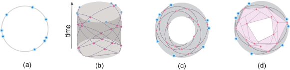
Figure 3: Construction of encounter complex: (a) Nodes (blue dots) moving on a circle $S^{1}$ and (b) their encounters over time (pink dots) in the encounter space (cylinder $S^{1}\times\mathbb{R^{+}}$); (c) nodes moving on an annulus and (c) their corresponding encounter complex

Encounter Metric

Let $\mathcal{I}$ denote the set of all of the IDs assigned to sensing nodes. For moving nodes in the network, an encounter event $\mathcal{E}_{i}$ occurs at time $t_{i}$ if $\exists\,I_{i}^{1},I_{i}^{2}\in\mathcal{I}$ such that $\|p(I_{i}^{1},t_{i})-p(I_{i}^{2},t_{i})\|\leq r_{d}$, where $p:(\mathcal{I},R)\mapsto\mathbb{R}^{2}$ is a coordinate function such that $p(i,t)$ is the position vector of the node $i$ at time $t$. The encounter $\mathcal{E}_{i}$ is represented as a tuple

$$\mathcal{E}_{i}=[t_{i},I_{i}^{1},I_{i}^{2}],$$ (1)

and its corresponding ID set is defined as $I_{i}=\{I_{i}^{1},I_{i}^{2}\}$. To build a distance metric on the set of encounter events, we construct an undirected weighted graph $\mathcal{G}$ with vertices corresponding to the events $\mathcal{E}_{i}$, denoted as encounter graph. For each two vertices $\mathcal{E}_{i}$ and $\mathcal{E}_{j}$, they are considered connected if $I_{i}\cap I_{j}\neq\emptyset$, and disconnected otherwise. The condition $I_{i}\cap I_{j}\neq\emptyset$ implies that there exist a node $k\in\mathcal{I}$ which has encountered two other agents at times $t_{i}$ and $t_{j}$ at positions $p_{i}$ and $p_{j}$, respectively. Due to the sensing limitations, these coordinates are not available at the base station. However, the Euclidean distance between $p_{i}$ and $p_{j}$ is bounded by $u_{ij}=v_{m}.|t_{i}-t_{j}|$, where $v_{m}=max(v_{c},v_{p})$. Therefore, one can assign a weight proportional to $u_{ij}$ as a rough estimation of $\|p_{i}-p_{j}\|$ to the undirected edge connecting $\mathcal{E}_{i}$ and $\mathcal{E}_{j}$ as $w_{ij}=\begin{cases}|t_{i}-t_{j}|,&\text{if }\mathcal{I}_{i}\cap\mathcal{I}_{j}\neq\emptyset\\ \infty,&\text{otherwise}\end{cases}$. Now we build a metric on $\mathcal{G}$, denoted by $\mathcal{D}_{\mathcal{G}}$, as $[\mathcal{D}_{\mathcal{G}}]_{i,j}=d_{\mathcal{G}}(\mathcal{E}_{i},\mathcal{E}_{j})$ where $d_{\mathcal{G}}(\mathcal{E}_{i},\mathcal{E}_{j})$ represents the length of the shortest path between nodes $\mathcal{E}_{i},\mathcal{E}_{j}$ in $\mathcal{G}$.

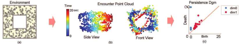
Figure 4: (a) An environment with one hole, (b) the encounter point cloud for data gathered over 20 seconds and (c) the persistence diagram

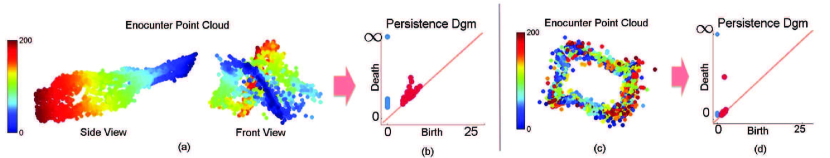
Figure 5: Comparison of the point clouds obtained from encounter data collected over 200 seconds using (a) encounter metric in the mobile network, (c) using contracted metric on the hybrid network, and their corresponding persistence intervals in (b) and (d), respectively.

Encounter Tracking

Due to the fact that the agents can have probabilistic stops in our model, taking into account every single encounter detection will result in redundant data. Therefore, we consider the encounters that take place only at the beginning of a period when two agents are in proximity with each other for the whole interval. Specifically, the encounter event $\mathcal{E}_{i}$ occurs at time $t_{i}$ if (i) $\exists I_{i}^{1},I_{i}^{2}\in\mathcal{I}$ such that $\|p(I_{i}^{1},t_{i})-p(I_{i}^{2},t_{i})\|\leq r_{d}$, and (ii) $\exists\,t^{\prime}\in[0,t_{i}]$ such that $\|p(I_{i}^{1},t)-p(I_{i}^{2},t)\|>r_{d}$ for $\forall t\in[t^{\prime},t_{i})$.

Figure 4 illustrates an example of a square environment with one hole inside on which 200 agents perform exploration. The encounter point cloud, colored over time of simulation, (figure 4(b)) resembles a noisy cylindrical tube, and one can easily distinguish the hole in the corresponding dgm${}_{1}(X)$ (figure 4(c)). However, as we continue data collection for a longer time interval, the cycles in its two ends tend to get deformed and the point cloud loses its cylindrical shape (figure 5(a)). In this case, the hole is not distinguishable from noise in the corresponding dgm${}_{1}(X)$ (figure 5(b)). We can justify this due to the accumulation of the errors in the encounter metric because of the uncertainty in pairwise distances over a long period of time, which makes the estimated point cloud gradually lose the topological structure existing in the real environment. Note that as it could be observed from figure 3(b), these encounters produce sampled points in the space of $\mathcal{D}\times[0,t_{f}]$, and collecting more observation over time does not help the estimation of $\mathcal{D}$ but it makes it worst. One solution to this problem would be to consider point clouds obtained from information over a shorter time frame that is still long enough to capture the correct structure. However, in practice, this would impose the requirement of tuning another parameter. In the following we will show that by adding an extra piece of information one can build more precise contracted point clouds that carry correct topological information without worrying about time frames.

Contracted Encounter Metric

To increase the precision of estimated pairwise distances in our metric, we consider the fact that the agents stop probabilistically for some time intervals, and keep track of stopped nodes in the network by asking the agents to transmit their change of moving status (RW, WF, or S). If two nodes meet the third one during one of its stop intervals, we infer the corresponding encounters have occurred at the same location. Hence we use this observation and improve the metric as follows: Let $\mathcal{T}_{k}=\{T_{k}^{1},T_{k}^{2},\dots\}$ be the set of stop intervals for agent $k$, meaning that agent $k$ has been in S mode for $\forall\,t\in T_{k}^{l},\,\forall l$. For two events $\mathcal{E}_{i}$ and $\mathcal{E}_{j}$, if $I_{i}\cap I_{j}=k$ and $t_{i},t_{j}\in T^{l}_{k}$ for some $l$, then we set $w_{ij}=0.$ We refer to this metric as a contracted encounter metric as it contracts the space of the corresponding encounter point cloud from $\mathcal{D}\times[0,t_{f}]$ to the lower dimension space of $\mathcal{D}$. We observed that contracting the point cloud improves the performance of the estimation in terms of more persistence features, but it still is not a complete embedding into a lower dimensional space as a result of the probabilistic nature of stop intervals of the agents.

A Hybrid Network

We can also make further improvements over the estimated metric by incorporating a few percentage of static nodes in the network, which we refer to it as a hybrid network. The exploration task initiates with all nodes starting in a RW status, and after a while, when the nodes are dispersed enough in the environment, a few percentage of them are commanded to stop as static nodes. Now, let $\mathcal{S}\in\mathcal{I}$ be the set of indices for these static nodes. Then we modify the corresponding weights for two encounter events $\mathcal{E}_{i}$ and $\mathcal{E}_{j}$ in case that $\mathcal{I}_{i}\cap\mathcal{I}_{j}\neq\emptyset$ as $w_{ij}=\begin{cases}\|t_{i}-t_{j}\|,&\text{if }I_{i}\cap I_{j}\notin\mathcal{S}\\ 0,&\text{if }I_{i}\cap I_{j}\in\mathcal{S}\\ \end{cases}$. This configuration can be used in case that the natural stop intervals of agents are not long enough to contract the point cloud space into a proper lower dimensional space. The resulting contracted point cloud and persistence diagrams for a hybrid network with only $\%5$ of static nodes are shown in figure 4(c) and (d), which nicely infer the existence of the environment by a much better separation between the persistent feature and the noise

Subsampling

In [20], we used the well-known maxmin landmark selection algorithm [24] for selecting a subset of point cloud on which the complexes are built. Unfortunately, maxmin filtration is very sensitive to outliers as they are distant from the other points in the set and very prone to be selected as the maximizers of the distance to the set of previously selected samples. Dealing with the outliers in real-world data analysis is of high importance. One of the causes of the appearance of outliers in the estimated data sets is due to the estimation uncertainties. In our problem, they occur as a result of inaccuracies in the estimation of encounter metric, which can be observed in figures 4 and 5. We propose two approaches to overcome this issue and improve the robustness of our mapping algorithm by enhanced filtration of the point cloud.

KNN filtering

In [25] nearest neighbor density estimation is used for pre-filtration of the point cloud. In our first approach, we employ a k-nearest neighbors (KNN) filtration followed by a maxmin subsampling algorithm to select a subsample of point cloud which preserves the topological information of the actual space and is robust to outliers. Specifically, for a point $x_{i}\in{X}$, let $d_{k}(x_{i})$ denote the distance between $x_{i}$ and it’s k-nearest neighbor, and $\overline{d}_{k}(x_{i})$ be the average distance to its k-nearest neighbors (inversely proportional to the local density of the point cloud around $x_{i}$). We consider the density of all average distances over ${X}$ as $\rho_{k}({X})$ and select the threshold $\tau_{q,k}$ to be $q$-quantile of $\rho_{k}({X})$. Then we select a subset $V$ of points $v_{i}$ such that $d_{k}(v_{i})<\tau_{q,k},\,\forall v_{i}\in V$, which will remove outliers of ${X}$ to a large extent. Finally, we apply the maxmin algorithm on the pre-filtered point cloud $V$ to obtain a smaller subset $V_{s}$ for persistence analysis.

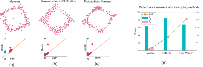
Figure 6: Comparison of (a) standard maxmin subsampling, (b) maxmin over pre-filtered data, and (c) probablistic maxmin algorithm, and (d) their SNR performance for 100 independent runs

Probabilistic maxmin

In the second approach, we propose a single stage sequential probabilistic subsampling method, where the local densities of the point cloud are taken into account directly in sequential sample selection procedure rather than in a separate pre-filtration process. We select the first sample $x_{1}\in{X}$ randomly; Then at each iteration, if $L$ is the set of the previously selected landmarks, find a point $l_{k}\in{X}$ such that it maximizes $\alpha(d(l_{k},L),\rho_{k}(l_{k}))$, where $\alpha(u,v)$ is a scalar continuous function with the properties: $\alpha(0,0)=0$, and $\alpha(u,.)$ is an increasing function of $u$ for a fixed $v$, $\alpha(.,v)$ is an increasing function of $v$ for a fixed $u$. An appropriate example of such a function for our application is $\alpha(u,v)=u+\omega v$ where $\omega$ is a constant scalar.

Figure 6(a-c) shows the subsampled point clouds of 150 points for a contracted data set in along with their persistence diagrams with parameters $q=0.9$ and $k=10$. It confirms that the one dimensional feature is more persistent using KNN filtration or our probabilistic maxmin subsampling than the standard maxmin approach. As another example, a subsampled point cloud from encounter information over a 2-hole square environment projected on 2D space is shown in figure 1. The points are colored according to the real positions of encounters in the environment, confirming that it nicely represents the structure of the environment. In order to compare the performance of landmark selection algorithms in presence of noise, we use a signal to noise ratio (SNR) measure as follows: For a point $(b^{i}_{n},d^{i}_{n})$ in dgm, let $l^{i}_{n}=[b_{n}^{i},d_{n}^{i}]$ be the corresponding persistence interval. Then $|l^{i}_{n}|$ represents the vertical distance of the point to the diagonal of dgm , and can be considered as a rough measure of significance or noisiness of features. In other words, features with small values of $|l^{i}_{n}|$ can be considered as noise and the ones with larger values as signals, with some level of confidence [16]. Let $\mathcal{L}_{n}=\{|l^{1}_{n}|,...,|l^{m}_{n}|\}$ be the set of all interval lengths in dimension $n$ sorted in non-decreasing order. Define the signal set as $\mathcal{S}_{n}=\{|l^{i}_{n}|\in\mathcal{L}_{n}\,|i<\beta_{n}+1\}$ and the noise set as the set difference $\mathcal{N}_{n}=\mathcal{L}_{n}\backslash\mathcal{S}_{n}$. Then their corresponding average powers can be defined as $P_{\mathcal{S}_{n}}=\frac{\sum_{\mathcal{S}_{n}}{|l_{n}^{i}|}^{2}}{|\mathcal{S}_{n}|}$ and $P_{\mathcal{N}_{n}}=\frac{\sum_{\mathcal{N}_{n}}{|l^{j}_{n}|}^{2}}{|\mathcal{N}_{n}|}$, and the signal to noise ratio as $SNR=\frac{P_{\mathcal{S}_{n}}}{P_{\mathcal{N}_{n}}}$. A number of $N$ independent subsampling runs can then be performed over the point cloud, and the average SNR can be used as the performance measure of the subsampling method. The average SNR measure for the scenario in figure 4 after 100 runs is shown in figure 6(d)exposing a great improvement of SNR for these approaches over the standard maxmin algorithm.

Robust Classification of Persistence Intervals

Betti numbers summarize topological features of a space $M$ as numbers. However, for a sampled point cloud $X$ out of $M$, one usually constructs a filtration of simplicial complexes on $X$ and analyzes varying homology over a scale space. For a dense enough sampled data, one can find a range of scales for which the homology of simplicial complexes is equal to the one for $M$ [16]. Nonetheless, persistence intervals do not provide a quantitative representation of the topology of the real space but only birth and death of the features over the scale space. Furthermore, we are interested in feature extraction algorithms that are robust to scaling and outliers. In the following part, we propose a density based classification algorithm for persistence intervals with the purpose of a scale invarient and robust feature extraction method for sampled data sets.

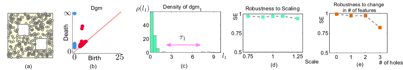
Figure 7: Robust Classification of persistence intervals: (a) A 2-hole environment, (b) the extracted persistence diagram, (c) density of persistence intervals with the appropriate threshold, (d) robustness of classification algorithm to scaling, and (e) to change in the number of features

Consider again the persistence interval lengths $|l^{i}_{n}|$. We are interested in finding a threshold for dimension $n$, $\tau_{n}$ such that all of the features with the property that $|l^{i}_{n}|>\tau_{n}$ can be considered as signals (see figure 7(d-e)). To make the approach scale invariant, we consider the density of interval lengths scaled by a $q_{n}$ quantile, $\rho_{q_{n}}(l_{n})$, and define the $n$-th Betti function as $\hat{\beta}_{n}(q_{n},\Delta_{n},\tau_{n})=\sum_{i}{\mathds{1}_{\mathbb{R}^{+}}\left(\frac{l^{i}_{n}}{l_{q_{n}}+\Delta_{n}}-\tau_{n}\right)},$ where $l_{q_{n}}$ is the $q_{n}$-quantile of the density, $\Delta_{n}$ has been added for dealing with singularities, and $\mathds{1}_{\mathbb{R}^{+}}(.)$ is the indicator function of ${\mathbb{R}^{+}}$ . Let $\mathbb{M}=\{M_{1},\ldots,M_{m}\}$ denote a set of random spaces that have the same topological characteristics as $M$, and $\mathbb{X}=\{X_{1},\ldots,{X_{m}}\}$ represent the corresponding set of sampled point clouds. Define the $(n,k)$-th Betti function as

$$\hat{\beta}^{k}_{n}(\Theta_{n})=\sum_{i}{\mathds{1}_{\mathbb{R}^{+}}\left(\frac{l^{i,k}_{n}}{l_{q_{n}}^{k}+\Delta_{n}}-\tau_{n}\right)},$$

and its corresponding error function as $e_{n}^{k}(\Theta_{n})=|\hat{\beta}^{k}_{n}(q_{n},\Delta_{n},\tau_{n})-\beta_{n}|$, where $\Theta_{n}=(q_{n},\delta_{n},\tau_{n})$ defines the parameter space. Now our classification problem reduces to perform an optimization algorithm to find the minimum of the cost functional $\mathcal{F}(\Theta_{n})=\left\|[e_{n}^{1}(\Theta_{n}),...,e_{n}^{m}(\Theta_{n})]^{T}\right\|_{1}/m$, i.e. the optimal parameter set is $\Theta^{*}_{n}=\operatorname*{arg\,min}_{\Theta_{n}}\mathcal{F}(\Theta_{n})$. To make the cost functional smooth for optimization purposes, one can replace the indicator function $\mathds{1}(.)$ with a sigmoid function $\sigma_{\alpha,l^{i}_{n}}(.)$ where $\sigma_{\alpha,x_{0}}(x)=\frac{1}{1+e^{-\alpha(x-x_{0})}}$.

We performed classification for dimension $1$ intervals on a training data set consisting of 100 variations of the space shown in figure 7(a) with random placements of the two square holes in the space. Persistence diagram and the corresponding density of interval lengths for one of the environments is shown in figure 7(b) and (c), respectively. The optimization process resulted in a minimum of $\mathcal{F}(\Theta^{*}_{1})=0.03$ with $\Theta^{*}_{1}=(0.5,0.7,3.7)$. This result is not surprising as the $0.5$-quantile of the density, which is the median of dataset, is known to be robust to outliers. To investigate the performance of our classifier, we evaluated $\mathcal{F}(\Theta^{*}_{1})$ for a variety of test sets $\mathbb{X}^{i}$, each containing 100 point clouds with random feature placements, with each test set differing in either scale of the environment and features or the number of features (holes). To investigate the performance, we used the sensitivity measure for classification, $SE=TP/(TP+FN)$, where $TP$ and $FN$ denote the number of true positives and false negatives, respectively. The sensitivity performance for these scenarios is summarized in figure 7 (d) and (e) for scaled environments, and environments with different numbers of holes but the same scale, respectively. Note that we have evaluated this measure for the whole mapping algorithm and not just for the classification part, which can justify the degradation in the performance for the 3-hole case, as we observed that in $15\%$ of the cases, the third hole could not be retrieved from the point cloud data.

Conclusion

We introduced encounter metrics for the construction of point clouds that represent topological features of unknown environments based on minimal encounter information of mobile nodes in a sensor networks whose mobility is inspired by insects. We enhanced the accuracy of the estimation with incorporating different pieces of information in the construction of the metric. Moreover, we employed density based subsampling approaches to cope with the outliers emerging due to uncertainties in the point cloud, and proposed a classification for robust feature extraction out of persistence diagrams. Future work includes validation of the proposed algorithms on swarm robotic and biobotic systems as well as the quantification of uncertainties in topological estimation. We are also working on how one can extract features other than connected components and holes from the encounter point cloud can be exploited for a more precise mapping technique.

References

- [1] K. Kotay, R. Peterson, and D. Rus, “Experiments with robots and sensor networks for mapping and navigation,” in Field and Service Robotics, vol. 25 of Springer Tracts in Advanced Robotics, pp. 243–254, 2006.
- [2] A. Mainwaring, D. Culler, J. Polastre, R. Szewczyk, and J. Anderson, “Wireless sensor networks for habitat monitoring,” Proceedings of the 1st ACM international workshop on Wireless sensor networks and applications - WSNA ’02, pp. 88–97, 2002.
- [3] G. A. Kantor, S. Singh, R. Peterson, D. Rus, A. Das, V. Kumar, G. Pereira, and J. Spletzer, “Distributed search and rescue with robot and sensor teams,” in The 4th International Conference on Field and Service Robotics, July 2003.
- [4] T. Balch and R. Arkin, “Behavior-based formation control for multirobot teams,” Robotics and Automation, IEEE Transactions on, vol. 14, no. 6, pp. 926–939, 1998.
- [5] J. Cortes, S. Martinez, T. Karatas, and F. Bullo, “Coverage control for mobile sensing networks,” Robotics and Automation, IEEE Transactions on, vol. 20, no. 2, pp. 243–255, 2004.
- [6] V. Gazi, “Swarm aggregations using artificial potentials and sliding mode control,” in Decision and Control, 2003. Proceedings. 42nd IEEE Conference on, vol. 2, pp. 2041–2046 Vol.2, 2003.
- [7] S. Gandhi, R. Kumar, and S. Suri, “Target counting under minimal sensing: Complexity and approximations,” in Algorithmic Aspects of Wireless Sensor Networks (S. Fekete, ed.), vol. 5389 of Lecture Notes in Computer Science, pp. 30–42, Springer Berlin Heidelberg, 2008.
- [8] J. Aulinas, Y. Petillot, J. Salvi, and X. Lladó, “The slam problem: a survey,” in Proceedings of the 2008 conference on Artificial Intelligence Research and Development, pp. 363–371, 2008.
- [9] Edelsbrunner H., D. Letscher, and A. Zomorodian, “Topological persistence and simplification,” Proceedings 41st Annual Symposium on Foundations of Computer Science, 2000.
- [10] H. Edelsbrunner and J. Harer, “Persistent homology-a survey,” Contemporary mathematics, vol. 0000, pp. 1–26, 2008.
- [11] H. Edelsbrunner and J. Harer, Computational Topology - an Introduction. American Mathematical Society, 2010.
- [12] R. Ghrist and a. Muhammad, “Coverage and hole-detection in sensor networks via homology,” IPSN 2005. Fourth International Symposium on Information Processing in Sensor Networks, 2005., no. 1, pp. 254–260.
- [13] V. de Silva and R. Ghrist, “Coverage in sensor networks via persistent homology,” Algebraic & Geometric Topology, vol. 7, pp. 339–358, 2007.
- [14] B. Walker, “Using persistent homology to recover spatial information from encounter traces,” in Proceedings of the 9th ACM international symposium on Mobile ad hoc networking and computing, MobiHoc ’08, p. 371, ACM Press, May 2008.
- [15] E. Munch, P. Bendich, and K. Turner, “Probabilistic Fr’{e} chet Means and Statistics on Vineyards,” arXiv preprint arXiv:1307.6530, pp. 1–25, 2013.
- [16] S. Balakrishnan, B. Fasy, and F. Lecci, “Statistical Inference For Persistent Homology,” arXiv preprint arXiv:1303.7117v1, 2013.
- [17] E. Chambers, V. Silva, J. Erickson, and R. Ghrist, “Vietoris–rips complexes of planar point sets,” Discrete and Computational Geometry, vol. 44, no. 1, pp. 75–90, 2010.
- [18] A. Zomorodian and G. Carlsson, “Computing persistent homology,” Proceedings of the twentieth annual symposium on Computational geometry - SoCG ’04, p. 347, 2004.
- [19] R. Jeanson, C. Rivault, J.-L. Deneubourg, S. Blanco, R. Fournier, C. Jost, and G. Theraulaz, “Self-organized aggregation in cockroaches,” Animal Behaviour, vol. 69, pp. 169–180, Jan. 2005.
- [20] A. Dirafzoon and E. Lobaton, “Topological Mapping of Unknown Environments using an Unlocalized Robotic Swarm,” in International Conference on Intelligent Robots and Systems (IROS), 2013, To appear.
- [21] T. Latif and A. Bozkurt, “Line following terrestrial insect biobots,” Engineering in Medicine and Biology Society (EMBC), 2012 Annual International Conference of the IEEE, pp. 972–975, Aug. 2012.
- [22] D. Morozov, “Dionysus library for persistent homology.” Software available at http://mrzv.org/software/dionysus.
- [23] T. F. C. M. Cox, Multidimensional Scaling. Chapman and Hall / CRC, 2nd ed., 2000.
- [24] V. D. Silva and G. Carlsson, “Topological estimation using witness complexes,” Proc. Sympos. Point-Based Graphics, 2004.
- [25] G. Carlsson, T. Ishkhanov, V. Silva, and A. Zomorodian, “On the Local Behavior of Spaces of Natural Images,” International Journal of Computer Vision, vol. 76, pp. 1–12, June 2007.