How accurate are stellar ages
based on stellar models?
II. The impact of asteroseismology

Abstract

Accurate and precise stellar ages are best determined for stars which are strongly observationally constrained, that is which are intrinsically oscillating. We review here the seismic diagnostics which are sensitive to stellar ages and provide some illustrating examples of seismically age-dated stars.

1 Introduction

Figure 1: Regions in the HR diagram where oscillating stars are observed. [From J. Christensen-Dalsgaard, http://astro.phys.au.dk/~jcd/oscilnotes/contents.html.]

Precise and absolute stellar ages are crucial requirements in many astrophysical studies. In particular, the huge harvest of newly discovered exoplanets calls for accurate and precise ages of their host-stars, a crucial parameter in the understanding of planet formation and evolution (Havel et al., 2011, see also the chapter by T. Guillot).

As we discussed in Part I, the determination of the age of a single star is very imprecise when the only observational data available for that star are its luminosity, effective temperature, and metallicity. Fortunately, there are several kinds of stars for which additional observational data are available, allowing to better constrain stellar models and thus to improve age-dating. Stellar masses can be obtained directly, via the third Kepler law, for stars in binary systems (visual/interferometric binaries or combined spectroscopic/eclipsing binaries). On the other hand, stellar radii are accessible for stars in combined eclipsing/spectroscopic binaries or, for bright or large stars observed in interferometry. Furthermore, major steps towards the precise and accurate age-dating (and weighing) of oscillating stars have been made after the asteroseismic data provided by the ultra high precision photometric space-borne missions CoRoT (Baglin et al., 2002) and Kepler (Koch et al., 2010) have been made available.

As illustrated in Fig. 1, stellar pulsations are observed in stars spanning the whole Hertzsprung-Russell (HR) diagram. The analysis of the observed frequencies allows to probe the physical processes that are at work in the propagation regions at the actual age of the star, but also that were at work in its past life. This was demonstrated a very long time ago, by the study of large amplitude, radial, classical pulsators as Cepheids (starting with the work of Eddington, 1917) and by helioseismology, following the discovery of low-amplitude pulsations in the Sun by Evans & Michard (1962) and Leighton et al. (1962). The field of asteroseismology slowly evolved after the first observation of low amplitude solar-like oscillations in Procyon (Brown et al., 1991), but made significant advances with the advent of ultra-high precision photometry conducted in space by CoRoT and Kepler. Indeed, these missions have detected low amplitude stellar oscillations in many stars allowing to measure their frequencies with a typical precision of a few tenths of micro Hertz (, Michel et al., 2008; Chaplin & Miglio, 2013).

Seismic data have been used to age-date and weigh many stars. Currently, two approaches are taken. The first one, ensemble asteroseismology, attempts to determine the age and mass of large sets of stars based on their mean seismic properties (Chaplin et al., 2014). In this approach, interpolation in large grids of “ready-made” stellar models, by different techniques, provides the mass and age of the model that best matches the observations. The alternative approach, more precise, is the hereafter named “à la carte” modelling (Lebreton, 2013), that is the detailed study of specific stars, one by one, also referred to as “boutique” modelling (see , Soderblom, 2013). This approach has been used to model CoRoT and Kepler stars (see the reviews by Baglin et al., 2013; Chaplin & Miglio, 2013). In particular, stars hosting exoplanets have been modelled by for instance Gilliland et al. (2011), Lebreton (2012), Escobar et al. (2012), Lebreton (2013), Gilliland et al. (2013), and Lebreton & Goupil (2014).

In this lecture, we focus on asteroseismic diagnostics of stellar ages and also briefly discuss the impact of asteroseismology in stellar mass and radius determination. We mainly restrict the subject to low-amplitudes oscillations in solar-like oscillators, that is damped oscillations stochastically excited by turbulence in the near surface layers. We concentrate on the advantages brought by the calculation of à la carte stellar models with respect to ensemble asteroseismology. The idea is to perform à la carte modelling of the stars with the strongest and more numerous observational constraints, which we refer to as calibrators. Calibrator modelling is expected to provide new insights and constraints on the complex physical processes at work in stellar interiors as well as on some of the unknown or -at least- very imprecise properties of any star, as its initial helium content. As discussed in details in Lecture 1, the poor knowledge we have of these aspects is responsible for large uncertainties in the age-dating of individual stars. The characterization of calibrators will then serve to improve the modelling and age-dating of other, less well-observed stars, in particular for statistical studies (for instance for Galactic structure and evolution studies). In the future, one can expect that a sufficient number of calibrators is known, paving the HR diagram in all its dimensions (mass, age/evolutionary stage, and chemical composition). Therefore, to any ordinary star will correspond a referent calibrator to be used to improve its characterization.

This chapter is organized as follows. In Section 2, we give a definition for à la carte stellar models and present some examples. In Section 3, we briefly present oscillation frequency calculations and we detail the different seismic diagnostics that are currently used to constrain stellar models and their ages. In Section 4, we present selected examples of age-dating based on asteroseismology and discuss the range of precision and accuracy that can be reached.

2 “À la carte” stellar modelling

In à la carte modelling, dedicated internal structure models are built to best represent the observed star. Given the observational data available for that star, an optimization process is conducted to define and calculate the stellar model that best matches these data. In the following, we distinguish so-called classical observational parameters from seismic ones. Classical parameters are, for instance, the effective temperature $T_{\mathrm{eff}}$, the luminosity $L$, the metallicity [Fe/H] or the individual abundances, the surface gravity $\log g$, and when measurable, the mass $M$, the radius $R$, the mean density derived from the transit of an exoplanet, etc. Seismic parameters can be the individual oscillation frequencies or different combinations of them (see Sect. 3.5). In the optimization process, an adjustment of the input physics and other parameters of the stellar models (, the initial helium abundance) is performed, to match at best the observations. Naturally, the more observational constraints, the more model parameters can be adjusted, as illustrated in the following.

The modelling of calibrators (Sun, very well-observed stars) is mainly performed à la carte. As recalled below, the solar model and other calibrator models provide the reference for modelling other stars, in terms of input physics, helium abundance, etc. Reference models also serve to calibrate empirical relations (for empirical age-dating, see the chapter by R. Jeffries). À la carte stellar models are also required when a precise characterization of an individual star is required, for instance when absolute ages are demanded. This is the case of exoplanet host-stars, for which we need the age, mass, and radius to characterize the exoplanet internal structure, formation scenario, and evolution (see the chapter by T. Guillot).

2.1 The Sun

The first calibrator ever studied is the Sun, see, for instance, the first paper on the helium content of the Sun by Schwarzschild (1946) where he found a mass fraction of helium $Y\approx 0.40$ and suggested an upper limit on the solar metallicity $Z/X$ of 0.255, , about ten times the present one, inferred from both the solar spectrum and analysis of meteorites! The solar model is a reference and provides tests and calibration for the physical description and free parameters of stellar models. In the case of the Sun, the classical parameters (mass $M_{\odot}$, radius $R_{\odot}$, luminosity $L_{\odot}$, individual abundances of chemical elements, age $t_{\odot}$) are very precisely measured. One commonly defines the standard solar model as the model of one solar mass that matches, at solar age, the observed solar luminosity, radius, and surface metallicity. The standard solar model is based on standard input physics, that is currently accepted and updated physical inputs at the time of the calculation. Once the input physics has been fixed, the calibration provides an estimate for the two main free parameters of the model, the initial helium content, which mainly controls the luminosity, and the mixing-length parameter of convection $\alpha_{\mathrm{conv}}$, which mainly controls the radius (see for instance works by Mazzitelli, 1979; Hejlesen, 1980; Christensen-Dalsgaard, 1982; Lebreton & Maeder, 1986). A few decades ago, the so-called solar neutrino problem bothered solar modellers (see , Bahcall & Shaviv, 1968) and some of them designed so-called non-standard solar models in order to reproduce the observed neutrino flux, see for instance the solar models with turbulent diffusion by Schatzman et al. (1981); Lebreton & Maeder (1987), or the exotic solar model with a central black hole by Stothers & Ezer (1973). This was prior to the finding that neutrinos have a mass and oscillate in three flavours in their travelling from Sun to Earth.

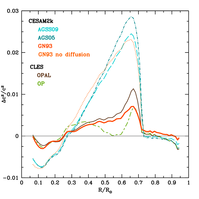
Figure 2: Relative differences between the sound speed derived through inversion of oscillation frequencies by Basu et al. (2000) and the sound speed obtained in different solar models. The inputs of solar models are discussed in Part I. [From Y. Lebreton, in the collective book by Stasińska et al. (2012).]

Very importantly, a major step towards the resolution of the solar neutrino problem came for helioseismology. Indeed, the very complete and precise set of solar pressure mode oscillation frequencies (see Sect. 3) provided by radial velocity and intensity measurements brought strong clues that the standard solar model, even imperfect, was not so far from reality (see , the review by Bahcall & Ulrich, 1988). Heliosismic analysis allowed to determine the present helium abundance in the solar convective envelope (, Gough, 1984; Dappen & Gough, 1984; Basu & Antia, 1995) as well as the depth of this envelope (Kosovichev & Fedorova, 1991; Christensen-Dalsgaard et al., 1991). In turn, this brought constraints on the input physics to be included in a solar model, mainly the gravitational settling of chemicals (Richard et al., 1996) and elaborated equations of state (Christensen-Dalsgaard et al., 1988). However, as illustrated in Fig. 2, there remained disagreements between the sound speed profile inferred from the inversion of the observed frequencies and the one obtained in solar models, in particular in the radiative regions just below the convective envelope and in the centre. Maximum relative differences in the square of the sound speed, $(c^{2}_{\mathrm{models}}-c^{2}_{\mathrm{observed}})/c^{2}_{\mathrm{observed}}$ are of $\sim 0.4$ per cent below the convective zone (, Christensen-Dalsgaard et al., 1996). These differences can partially be erased by the introduction of a transport of chemical elements in the radiative zone (Gabriel, 1997). More recently, Zhang & Li (2012) showed that the disagreement in the sound speed between solar models and helioseismic inversions below the base of the solar convective envelope nearly disappears when diffusive overshooting mixing is taken into account at the transition between the upper convective layers and the lower radiative interior (see also Christensen-Dalsgaard et al., 2011).

Helioseismology still calls for further improvements and refinements in the solar model description, regarding for instance internal rotation (see Schou et al., 1998; Chaplin et al., 1999), and the description of the tachocline (see Rogers, 2011, for a review). Furthermore, the redetermination of the solar abundances on the basis of 3-D model atmospheres and improved atomic data led to a degradation of the quality of the modelling of the sound speed profile. With the new AGSS09 abundances (presented in Lecture 1), the difference $(c^{2}_{\mathrm{models}}-c^{2}_{\mathrm{observed}})/c^{2}_{\mathrm{observed}}$ is about $10$ times larger than in the Christensen-Dalsgaard et al. (1996) solar model based on the GN93 mixture (see , Asplund et al., 2009, and Fig. 2). Finally, gravity modes which would allow to probe the deep interior of the Sun (see Sect. 3 below) are still tracked, but their low amplitudes make the quest difficult (, García et al., 2007).

2.2 Other stars

For other stars, we are quite far from the degree of achievement of the solar model. We actually assume solar values for the free parameters entering their physical description, even if they may have masses, chemical compositions, and evolutionary stages far from solar. However, when the observational data are very precise and numerous, the status of calibrator can be given to a star. Then, with à la carte modelling, we hope to reach a level where we are able to discriminate different options for the input physics of stellar models and get insight on mostly free parameters, as the helium content. For stellar calibrators, the age determination will therefore be not only more precise, but also more accurate. We give some examples later in the text.

2.3 Optimization procedures

In seismic à la carte modelling, the constraints on the classical observed stellar parameters and those on the seismic ones are combined to improve the calibration of the model of the considered star. In the examples presented in Sect. 4, $L$, $T_{\mathrm{eff}}$, [Fe/H] will be considered together with different seismic indicators. Then, stellar models are calculated and their unknowns, which may be either inputs or outputs of the model calculation, are adjusted so as to minimize the deviation of the model from the observational material. The goodness of the match can be evaluated through the minimization of a merit function $\chi^{2}$, which can be written,

$$\chi^{2}\;=\;\sum_{i=1}^{N_{\mathrm{obs}}}\frac{\left(x_{\mathrm{i,mod}}-x_{\mathrm{i,obs}}\right)^{2}}{\sigma_{\mathrm{i,obs}}^{2}}\,,$$ (1)

where $N_{\mathrm{obs}}$ is the total number of observational constraints considered, $x_{\mathrm{i,mod}}$ and $x_{\mathrm{i,obs}}$ are the computed and observed values of the $i^{\mathrm{th}}$ constraint. The more observational constraints available, the more free parameters can be adjusted in the modelling process. The parameters that are currently adjusted are the initial stellar mass $M$, the initial $(Z/X)_{0}$ and helium mass fraction $Y_{0}$ (all are models inputs), the parameters entering the physical description of the star (mainly the mixing-length parameter of convection $\alpha_{\mathrm{conv}}$ and overshooting parameter $\alpha_{\mathrm{ov}}$), and the age $A$ (model output). If too few observational constraints are available, some free parameters have to be fixed (see below), while the others can be adjusted. Note that the expression of the $\chi^{2}$ in Eq. 1 is not valid if data are correlated. In that case, Eq. 35 has to be used (see Sect. 3.5.7).

Different optimizations approaches have been used to adjust stellar models to observational constraints: model-grid based methods (Stello et al., 2009; Quirion et al., 2010, etc.), genetic algorithms as in the Asteroseismic Modelling Portal (Metcalfe et al., 2009), Levenberg-Marquardt minimization (Miglio & Montalbán, 2005), and Bayesian approach (Gruberbauer et al., 2012; Bazot et al., 2012). The Levenberg-Marquardt (LM) algorithm combines the steepest descent method and Newton’s method to solve non-linear least square problems (Bevington & Robinson, 2003; Press et al., 2002). In some examples presented below the LM minimization method was used in the way described by Miglio & Montalbán (2005).

3 Stellar oscillations

3.1 Setting the stage

Pulsating stars are spanned all across the HR diagram (Fig. 1). There are many categories of oscillators both in terms of the kind of pulsations observed (radial or non-radial), and of their amplitudes and driven mechanism. In particular, one distinguishes pulsating stars where the amplitudes of the oscillations are large (Cepheids, Mira, etc.) from low-amplitude pulsators (solar-like, $\beta$ Cephei, etc.). The characteristic oscillation period $P$ scales as the dynamical time-scale $t_{\mathrm{dyn}}$, which measures the amount of time it would take a star to collapse in the absence of any internal pressure. Therefore $P$ reads,

$$P\approx t_{\mathrm{dyn}}\;=\;\left(\frac{2R^{3}}{GM}\right)^{1/2}\propto\langle\rho\rangle^{-1/2}\quad.$$ (2)

The theory of stellar oscillations is presented and detailed in text books, see , Cox (1980), Unno et al. (1989), Christensen-Dalsgaard (2014), Aerts et al. (2010), and references therein. In the following, we only briefly recall the main steps of the calculation of stellar oscillations. We focus on solar-like oscillations, excited by stochastic convective motions that take place in low-mass stars. The related oscillators are multi-mode oscillators.

3.2 Stellar oscillations equations

The structure of a star is described with the classical equations of hydrodynamics,

$$\frac{\partial\rho}{\partial t}+\overrightarrow{\nabla}.(\rho\vec{u})\;=\;0,\ \hfill\ \mathrm{continuity}$$ (3)

$$\rho\left(\frac{\partial}{\partial t}+\vec{u}.\overrightarrow{\nabla}\right)\vec{u}\;=\;\rho\vec{f}-\overrightarrow{\nabla}P-\rho\overrightarrow{\nabla}\Phi+\mathop{\mathrm{div}}\mathfrak{S},\ \hfill\ \mathrm{momentum}$$ (4)

with

$$\Delta\Phi\;=\;{\nabla}^{2}\Phi=4\pi G\rho,\hfill\mathrm{Poisson^{\prime}s\ equation}$$ (5)

$$\rho T\left(\frac{\partial}{\partial t}+\vec{u}.\overrightarrow{\nabla}\right){S}\;=\;\rho(\epsilon_{\mathrm{nuc}}+\epsilon_{\mathrm{visc}})-\overrightarrow{\nabla}.\overrightarrow{F_{\mathrm{R}}},\hfill\mathrm{energy\ conservation}$$ (6)

where $\rho$ is the density, $P$ the pressure, $T$ the temperature, $\vec{u}$ the velocity of the flow, $\vec{f}$ the external forces, $\Phi$ the gravitational potential, $\mathfrak{S}$ the viscous stress tensor, $\overrightarrow{F_{\mathrm{R}}}$ the heat flux, $S$ the entropy, and $\epsilon_{\mathrm{nuc,visc}}$ the energy produced or lost by nuclear reactions, neutrino loss, viscous heat generation, etc.

The basic assumptions consist in neglecting external forces, dissipation, and shear instabilities. Furthermore, oscillations occur on a dynamical time scale, which in the evolutionary phases of interest here is much smaller than both the Kelvin-Helmholtz and nuclear time scales (see definitions in Lecture 1). Oscillations can then be treated as small perturbations of the equilibrium model at a given evolutionary stage. Hereafter, the variables defining the equilibrium state of the star are labelled with the subscript $0$ ($\vec{u_{0}}=\vec{0}$, $p_{0}$, $\rho_{0}$, etc.). The equations are then linearised in the perturbations with a classical time dependency in $\exp(-i\omega t)$. The linear perturbations associated with the oscillations are then defined as

$$\vec{\xi}(\vec{r},t)\;=\;\vec{\xi}(\vec{r})\,\exp(-i\omega t),$$ (7)

where $\vec{\xi}(\vec{r})$ is the radial displacement vector. The velocity and pressure read,

$$\vec{u}(\vec{r},t)\;=\;-i\,\omega\ \vec{\xi}(\vec{r})\ \exp(-i\omega t)\ ;\ p(\vec{r},t)=[p_{0}(\vec{r})+p^{\prime}(\vec{r})]\exp(-i\omega t)\;,$$ (8)

where $p^{\prime}(\vec{r})$ is the pressure perturbation, etc. The horizontal dependence of the functions is then expressed using the spherical harmonics, for instance for the pressure perturbation,

$$p^{\prime}(\vec{r})\;\propto\;p^{\prime}({r})\times Y_{\ell}^{m}(\theta,\phi),\ \mathrm{etc.}$$ (9)

where $\theta$ and $\phi$ denote the usual spherical coordinates. This provides an equation for the radial displacement

$$-\omega^{2}\rho_{0}\xi_{r}+\dfrac{\mathrm{d}p^{\prime}}{\mathrm{d}r}+\rho_{0}\dfrac{\mathrm{d}\Phi^{\prime}}{\mathrm{d}r}+\rho^{\prime}g_{0}=0\;,$$ (10)

as well as associated equations for the perturbations of the Poisson’s equation and continuity equation.

In a third step, the heat exchanges may be discarded, which does not impact the frequencies significantly. In such an adiabatic approximation

$$\dfrac{p^{\prime}}{p_{0}}\;=\;\Gamma_{1}\dfrac{\rho^{\prime}}{\rho_{0}}\,,$$ (11)

where

$$\Gamma_{1}\;=\;\left(\dfrac{\partial\ln p}{\partial\ln\rho}\right)_{\mathrm{ad}}\;,$$ (12)

is the first adiabatic exponent.

The surface and central properties of a star allow standing waves to develop, which are at the origin of the observed surface oscillations. In the case of pressure modes for instance, modes are reflected at the surface because of the decrease of the density, and are refracted on the inner boundary of the trapping cavity because of the inwards increase of the (adiabatic) sound speed ${c}_{\mathrm{s}}=\sqrt{\Gamma_{1}p/\rho}$. Note that for an ideal gas, ${c}_{\mathrm{s}}\propto\sqrt{T/\mu}$, where $\mu$ is the mean molecular weight. Mathematically, boundary conditions must be imposed when solving the oscillation equations; the problem of stellar oscillations is therefore an eigenvalue problem. The solution is a set of discrete frequencies $\nu_{n,\ell,m}=\omega_{n,\ell,m}/2\pi$, each frequency being characterized by three numbers (integers).

The radial dependence of an eigenfunction is characterized by the number $n$, the radial order, which counts the number of nodes along a stellar radius. The horizontal dependence is represented by the spherical harmonic $Y_{\ell,m}$. The number $\ell$ is the angular degree, it counts the number of nodal lines on the surface, while $m$ is the azimuthal order, which counts the number of nodal lines crossing the equator. In absence of rotation, modes of same $n$, $\ell$, and different $m$ have the same frequency. We neglect rotation in the following and therefore write $\nu=\nu_{n,\ell}$.

We point out that the observations of CoRoT and Kepler have provided sets of oscillation frequencies $\nu_{n,\ell}$ for many stars with a very high precision. These frequencies are distance-independent and provide very strong constraints for the modelling of oscillating stars.

3.3 Nature of the oscillation modes

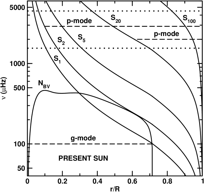
Figure 3: Propagation diagram for the Sun. The profiles of the buoyancy $N^{2}_{\mathrm{BV}}$ and of the acoustic frequency $S^{2}_{\ell}$, this latter for different values of the angular degree $\ell$, are plotted. Horizontal dotted lines delimit the frequency range of observed solar oscillations. From top to bottom, dashed lines span the cavities where $p$-modes with $\ell=20$ and $\ell=2$ are trapped, and the region of propagation of a gravity mode. [From Lebreton & Montalbán (2009).]

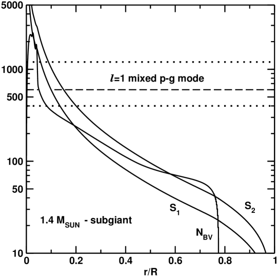
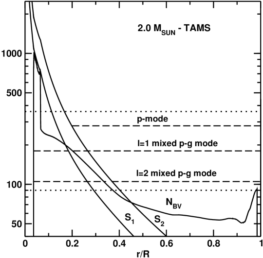
Figure 4: Propagation diagrams, as in Fig. 3 for different stellar masses. Top: star of mass $M=1.4\ M_{\odot}$ in the subgiant stage. Bottom: star of mass $M=2\ M_{\odot}$ at the end of its MS phase, close to the TAMS. The frequency domains (dotted lines) and regions of propagation of $p$-modes and mixed $p-g$ modes (dashed lines) are indicated. [From Lebreton & Montalbán (2009).]

A further simplification of the problem, called the Cowling approximation (Cowling, 1941), consists in neglecting the perturbations of the gravitational potential $\Phi$. For what concerns the present lecture, it is valid at large values of the absolute value of the radial order $n$. Moreover, some more approximations can be made, which consist in neglecting the terms containing derivatives of the equilibrium quantities (, Aerts et al., 2010, pages 203-204). With these approximations, the differential equation governing the radial displacement is of second order and reads,

$$\frac{\mathrm{d}^{2}\xi_{r}}{\mathrm{d}r^{2}}+K_{r}\xi_{r}\;=\;0\;,$$ (13)

with

$$K_{r}\;=\;\frac{1}{\omega^{2}{c}_{\mathrm{s}}^{2}}\left(N^{2}_{\mathrm{BV}}-\omega^{2}\right)\left(S^{2}_{\ell}-\omega^{2}\right)\;,$$ (14)

where $N^{2}_{\mathrm{BV}}$ and $S^{2}_{\ell}$ are characteristic frequencies defined below. The nature of the solution depends on the sign of $K_{r}$. When $K_{r}>0$, the solution is an oscillating wave, while when $K_{r}<0$ the solution is an exponential function and the wave is evanescent. In the adiabatic approximation, the frequencies only depend on two quantities (for instance $c_{\mathrm{s}}$ and $\rho$).

Two characteristic frequencies appear in Eq. 13. The critical acoustic frequency, or Lamb frequency reads,

$$S^{2}_{\ell}\;=\;\dfrac{\ell(\ell+1)c_{\mathrm{s}}^{2}}{r^{2}}\quad.$$ (15)

It characterizes the compressibility of the medium. Note that $S^{2}_{\ell}$ depends on the chemical composition inside the star, via the dependence in $\mu$ of the sound speed. Therefore, it is related to the evolutionary stage and age of the star. The buoyancy $N^{2}_{\mathrm{BV}}$, or Brunt-Väisälä (BV) frequency, reads,

$$N^{2}_{\mathrm{BV}}\;=\;g\left(\frac{1}{\Gamma_{1}}\,\frac{\mathrm{d}\ln p}{\mathrm{d}r}-\frac{\mathrm{d}\ln\rho}{\mathrm{d}r}\right)\;.$$ (16)

In a radiative zone, $N^{2}_{\mathrm{BV}}>0$. It is the frequency associated to the oscillation of a perturbed parcel of a gravitationally stratified fluid. In a convective zone $N^{2}_{\mathrm{BV}}<0$. Furthermore, for an ideal gas,

$$N^{2}_{\mathrm{BV}}\;=\;\frac{g^{2}\rho}{p}\left(\nabla_{\mathrm{ad}}-\nabla+\nabla_{\mu}\right)\;,$$ (17)

where $\nabla=(\mathrm{d}\ln T/\mathrm{d}\ln p)$ denotes the actual temperature gradient, $\nabla_{\mathrm{ad}}$ the adiabatic gradient, and $\nabla_{\mu}=(\mathrm{d}\ln\mu/\mathrm{d}\ln p)$, the gradient of the chemical composition. In a star interior, the profile of $N^{2}_{\mathrm{BV}}$ reflects density changes, and chemical composition changes via the gradients of the chemical composition built by the evolution.

The solution of Eq. 13 is an oscillatory one when

• $\lvert\omega\rvert>\lvert N_{\mathrm{BV}}\rvert$ and $\lvert\omega\rvert>\lvert S_{\ell}\rvert$. In that case, the solution corresponds to standing (acoustic) pressure waves, commonly called $p$-modes, for which the restoring force is related to the pressure gradient.

• $\lvert\omega\rvert<\lvert N_{\mathrm{BV}}\rvert$ and $\lvert\omega\rvert<\lvert S_{\ell}\rvert$. In that case, the solution corresponds to standing gravity waves, commonly called $g$-modes, for which the restoring force is related to the buoyancy.

The kind of possible solutions in a star like the Sun are illustrated in the propagation diagram in Fig. 3. It shows that in the Sun, pressure-modes of $\ell\geq 0$ can propagate up to the surface where they are observed, while gravity modes are predicted to propagate in the inner regions, but are evanescent in the convective envelope. Since the frequencies of the oscillation modes depend on the properties of the stars, propagation diagrams are different for different stellar masses, evolutionary stages (ages), and chemical compositions. This is illustrated in Fig. 4 where we show the propagation diagrams of a $1.4\ M_{\odot}$ star in the subgiant stage and of a $2\ M_{\odot}$ star at the end of its MS phase, close to the terminal age main sequence (TAMS). This latter would correspond to a A-star in the $\delta$ Scuti phase. We point out that the profiles of the buoyancy in these two stars differ from the solar one. During the MS, those stars possessed a convective core (still present in the $2\ M_{\odot}$ star). Because of nuclear evolution and convective core recession during the MS, a steep molecular weight gradient has been built in the inner regions producing the observed peak in $N_{\mathrm{BV}}$ (see Eq. 17). Furthermore, the increase of density in the central regions of the $1.4\ M_{\odot}$ model, resulting from core contraction on the subgiant branch leads to a central increase of $N_{\mathrm{BV}}$, and therefore of the frequencies of possible $g$-modes. In these slightly evolved stars, the range of frequencies of gravity modes overlap the one of pressure modes, while the evanescent region between the $g$-mode trapping cavity and the $p$-mode one is narrower.

When the intermediate evanescent region is narrow enough, one $g$-mode and one $p$-mode which happen to have very close frequencies actually are no longer a pure $g$-mode and a pure $p$-mode respectively. Instead both modes behave both as a $g$-mode in the inner cavity and as a $p$-mode in the outer cavity. This phenomenon called avoided crossing has been predicted and described by Scuflaire (1974) and Aizenman et al. (1977), and was first observed by Osaki (1975) in a $10\ M_{\odot}$ star. Such modes, that change their nature when propagating in the star, are called mixed $p-g$ modes. They carry information on the inner regions of the star (see the detailed description of the conditions of occurrence of these modes by Deheuvels & Michel, 2011). Mixed modes provide diagnostics on the compactness of stellar cores as well as on the different mixing processes at work during the evolution of a star. This is illustrated in Sect. 4.

Fig. 1 illustrates the variety of oscillation modes excited in different types of stars with different internal structures. The main oscillators are listed below.

• Solar-like oscillators: high radial order $p$-modes with periods spanning the range a few minutes (MS) to a few hours (red giants).

• $\gamma$ Doradus stars: high order $g$-modes, periods in the range $\approx$ 8 hours–3 days.

• $\delta$ Scuti stars: low order $p-g$ modes, periods in the range $\approx$ 30 minutes–6 hours.

• SPB stars: high order $g$-modes with periods in the range $\approx$ 15 hours–5 days.

• $\beta$ Cephei stars: low order $p-g$ modes with periods in the range $\approx$ 2–8 hours.

Figure 5: Stars where solar-like oscillations are detected, after Chaplin & Miglio (2013). Left: stars observed during CoRoT long runs, , 3 months of observation per star. Right: stars observed by Kepler for a total duration of 3 years observations per star.

3.4 Solar-like oscillators

The proximity of the Sun permits high temporal and spatial resolution observations. More than $10^{7}$ pressure modes have been observed and identified with angular degrees $\ell=0$ to $\sim 5000$. The high number of frequencies and the extremely high accuracy of the frequency measurements have allowed to conduct sophisticated studies. The inversion of the oscillation frequencies provided the profile of the sound speed, of the density, and of the rotation rate from the surface to regions close to the centre (see Sect. 2.1). From these studies, very accurate measurements were drawn, mainly the depth of the convective envelope and its helium content. In the case of stars different from the Sun, all kinds of modes may propagate depending on the star, that is either $p$, $g$, or $p-g$ mixed modes. However, because of the lack of spatial resolution and of measurements restricted to integrated light, the accessible modes are those with low angular degrees with $\ell$ in the range 0 to 3 at best. Inversions of oscillations have been performed for several red giants (RGs) and subgiants (SGs), which provided the rotation profile (see Sect. 4.2.2). A rich harvest of observational data has been provided by CoRoT and Kepler, as illustrated in Fig. 5.

3.5 Asteroseismic analysis and diagnostics

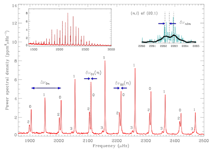
Figure 6: Kepler oscillation spectrum of the MS star 16 Cygni A. Top left-hand inset: frequency-power spectrum. Main plot: zoom on a range in frequency, indicating the frequency of maximum oscillation power, $\nu_{\mathrm{max}}$ at about 2200 $\mu$Hz, and the characteristic frequency separations discussed in the text. Top right-hand inset: zoom in frequency showing rotational frequency splitting of the non-radial $\ell=1$, $n=20$ mode (not discussed here). [From Chaplin & Miglio (2013).]

3.5.1 Individual oscillation frequencies

Figure 6, left-hand inset, from Chaplin & Miglio (2013), shows the frequency power spectrum of the solar-like oscillator 16 Cygni A, as observed by Kepler (Metcalfe et al., 2012). This power spectrum shows the now famous regular pattern of pressure modes observed in the Sun and in the many solar-like oscillators observed by CoRoT and Kepler. Another example is the frequency power spectrum of the CoRoT main target HD 43587 obtained by Boumier et al. (2014).

A formulation adapted from the asymptotic expansion by Vandakurov (1967) and Tassoul (1980) is commonly used to interpret the observed low-degree pressure mode oscillation spectra (see , Mosser et al., 2013, and references therein). It approximates the frequency of a $p$-mode of high radial order $n$ and angular degree $\ell{\ll}n$ as

$$\nu_{n,\ell}\;{\simeq}\;\left(n+\frac{1}{2}\ell+\epsilon\right)\Delta\nu_{\mathrm{asym}}-\ell(\ell+1)D_{0}\;.$$ (18)

Therefore, in the asymptotic approximation, $p$-modes of same angular degree and consecutive $n$ are nearly equidistant in frequency. The coefficients $\epsilon$, $\Delta\nu_{\mathrm{asym}}$, and $D_{0}$ depend on the considered equilibrium state of the star. In particular

$$\Delta\nu_{\mathrm{asym}}\;{=}\;\left(2\int\limits_{0}^{R}\frac{\mathrm{d}r}{c}\right)^{-1}\ \mathrm{and}\ \ D_{0}\approx-\frac{\Delta\nu_{\mathrm{asym}}}{4\pi^{2}\,\nu_{n,\ell}}\int\limits_{0}^{R}\frac{\mathrm{d}c}{r}\;.$$ (19)

The quantity $\Delta\nu_{\mathrm{asym}}$ measures the inverse of the sound travel time across a stellar diameter and is proportional to the square root of the mean density. The quantity $D_{0}$ probes the evolution status (and then age of the star) through the sound speed gradient built by the chemical composition changes in the stellar core.

The $\epsilon$ term weakly depends on $n$ and $\ell$, but it is much sensitive to the physics of surface layers. The problem is that outer layers in solar-type oscillators are the seat of inefficient convection, a 3-D, non-adiabatic, and turbulent process, which is poorly understood. The modelling of near surface stellar layers is uncertain and so are the related computed frequencies. These so-called near-surface effects are a main concern when using individual frequencies to constrain stellar models because they are at the origin of an offset between observed and computed oscillation frequencies. Some empirical recipes are used to correct for this offset. This is discussed below.

3.5.2 $\nu_{\mathrm{max}}$, $\langle\Delta\nu\rangle$ and scaling relations

From the oscillation power spectrum, the frequency at maximum amplitude $\nu_{\mathrm{max}}$ is extracted (see left-hand inset in Fig. 6 where $\nu_{\mathrm{max,16Cyg}}\simeq 2200~{}\mu\mathrm{Hz}$). This quantity is proportional to the acoustic cut-off frequency, itself related to effective temperature and surface gravity (see , Brown et al., 1994; Kjeldsen & Bedding, 1995; Belkacem et al., 2011). This dependency yields a scaling relation used to constrain the mass and radius (or surface gravity) of a star of known $T_{\mathrm{eff}}$,

$$\frac{\nu_{\mathrm{max,sc}}}{\nu_{\mathrm{max,\odot}}}\;{=}\;\left(\frac{M}{M_{\odot}}\right)\left(\frac{T_{\mathrm{eff}}}{5777\,K}\right)^{-1/2}\left(\frac{R}{R_{\odot}}\right)^{-2}\,=\,\left(\frac{g}{g_{\odot}}\right)\left(\frac{T_{\mathrm{eff}}}{5777\,K}\right)^{-1/2}\;,$$ (20)

where $\nu_{\mathrm{max,\odot}}=3050\ \mu$Hz is the solar value and the index $\mathrm{sc}$ stands for scaling.

The difference in frequency of two $p$-modes of same degree and consecutive orders reads

$$\Delta\nu_{\ell}(n)\;{=}\;\nu_{n,\ell}{-}\nu_{n-1,\ell}\,,$$ (21)

and is named the large frequency separation (see main panel of Fig. 6). The mean large frequency separation is used to constrain stellar models.

There are different ways to estimate the large frequency separation in a stellar model. First, it can be calculated as an average of the individual separations defined by Eq. 21. Second, in the asymptotic approximation (Eq. 18), $\Delta\nu_{\ell}(n){\equiv}\Delta\nu_{\mathrm{asym}}$ is approximately constant whatever the $\ell$ value. $\Delta\nu_{\mathrm{asym}}$ can therefore be derived from an adjustment of the asymptotic relation through the observed frequencies (for instance by a weighted least-squares fit). Such an adjustment also provides the values of $D_{0}$ and $\epsilon$. Third, as mentioned above, $\langle\Delta\nu\rangle\propto\langle\rho\rangle^{1/2}$. This yields a scaling relation usable to constrain stellar mass and radius (see , Ulrich, 1986; Kjeldsen & Bedding, 1995),

$$\frac{\langle\Delta\nu\rangle_{\mathrm{sc}}}{\langle\Delta\nu\rangle_{\odot}}{=}\left(\frac{M}{M_{\odot}}\right)^{1/2}\left(\frac{R}{R_{\odot}}\right)^{-3/2},$$ (22)

where $\langle\Delta\nu\rangle_{\odot}=134.9\ \mu$Hz is the solar value.

3.5.3 Small frequency separations and separation ratios

The difference in frequency of two pressure modes of degrees differing by two units and orders differing by one unit reads

$$d_{\ell,\ \ell+2}(n)\;{=}\;\nu_{n,\ell}{-}\nu_{n-1,\ \ell+2}\quad,$$ (23)

and is commonly referred to as the small frequency separation. According to the asymptotic relation (Eq. 18), $d_{02}(n)$ scales as ${\approx}6D_{0}$. Thus, $d_{02}(n)$ probes the central conditions, and in turn the evolutionary status of stars. The quantity $d_{02}(n)$, often also denoted by $\delta\nu_{02}(n)$, is shown in Fig. 6.

Modes of $\ell=1$ are rather easy to detect, while modes of $\ell=2$ are not always observed, or are affected by large error bars. This led Roxburgh & Vorontsov (2003) to propose to use either the three points small frequency separations $d_{01}(n)$ and $d_{10}(n)$, or the five points separations $dd_{01}(n)$ and $dd_{10}(n)$ as diagnostics for stellar models. These quantities read

$$d_{01}(n) = -\frac{1}{2}(\nu_{n-1,1}-2\nu_{n,0}+\nu_{n,1})\,$$ (24)

$$d_{10}(n) = \frac{1}{2}(\nu_{n+1,0}-2\nu_{n,1}+\nu_{n,0})$$ (25)

for the three points separations, and

$$dd_{01}(n) = \frac{1}{8}(\nu_{n-1,0}-4\nu_{n-1,1}+6\nu_{n,0}-4\nu_{n,1}+\nu_{n+1,0})\,,$$ (26)

$$dd_{10}(n) = -\frac{1}{8}(\nu_{n-1,1}-4\nu_{n,0}+6\nu_{n,l}-4\nu_{n+1,0}+\nu_{n+1,1})\,,$$ (27)

for the five points separations. An illustration is provided in Fig. 6 for the quantity $d_{01}(n)$ denoted by $\delta\nu_{01}(n)$. According to the asymptotic relation (Eq. 18), $dd_{01/10}(n)$ scales as ${\approx}2D_{0}$. Thus, these quantities also probe the central conditions, and in turn the evolutionary status of stars.

Furthermore, Roxburgh & Vorontsov (2003) demonstrated that, while the frequency separations are sensitive to near-surface effects, these effects nearly cancel in the frequency separation ratios defined as

$$r_{02}(n) = d_{02}(n)/\Delta\nu_{1}(n)\;,$$ (28)

$$rr_{01}(n) = dd_{01}(n)/\Delta\nu_{1}(n)\;,$$ (29)

$$rr_{10}(n) = dd_{10}(n)/\Delta\nu_{0}(n+1)\;.$$ (30)

Furthermore, the second difference $\delta_{2}\nu$ has been introduced by Gough (1990):

$$\delta_{2}\nu_{n,\ell}\;=\;\nu_{n+1,\ell}-2\nu_{n,\ell}+\nu_{n-1,\ell}\;,$$ (31)

and can be seen as a second derivative of the frequency $\nu_{n,\ell}$ with respect to $n$. This quantity is sensitive to rapid variations in the sound speed profile inside the star. Frequency separations and ratios can be used to constrain stellar models.

3.5.4 Period separations for $g$-dominated mixed modes

In the asymptotic theory (Tassoul, 1980), it is shown that the period difference between two pure $g$-modes of same degree and consecutive radial orders is approximately constant and reads,

$$\Delta P_{n,\ell}\;=\;P_{n+1,\ell}-P_{n,\ell}\;\propto\;\frac{n}{\sqrt{\ell(\ell+1)}}\Pi_{0}\;,$$ (32)

where

$$\Pi_{0}\;{=}\;\left(\ \int\limits_{r_{\mathrm{cc}}}^{R}\frac{\lvert N_{\mathrm{BV}}\rvert}{r}dr\right)^{-1}\;.$$ (33)

As discussed above, mixed $p-g$ modes develop in evolved solar-like stars reaching the end of the MS and beyond. The asymptotic approximation is no longer valid for mixed modes, nor for modes whose wavelength is longer than the length-scale of variations of the structure of the star in the region where they propagate. Therefore, the periods of mixed modes described in Sect. 3.3, or those of high-order $g$-modes propagating in a region with sharp features in $N_{\mathrm{BV}}$, may deviate with respect to the equidistant behaviour predicted by Eq. 32. The properties of this deviation allow us to probe the size of the convective core, mixed regions, and extra-mixing processes inside the star, as shown by Miglio et al. (2007), Miglio et al. (2008), Deheuvels & Michel (2011), see also Sect. 4.

3.5.5 Related seismic diagnostics

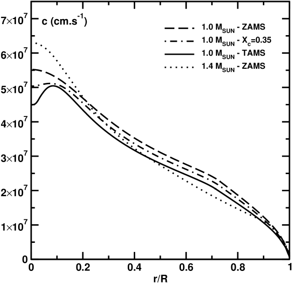
Figure 7: Top: the change of the mean density with evolution on the MS for three values of the stellar mass. Bottom: the sound speed profile in $1\ M_{\odot}$ and $1.4\ M_{\odot}$ models, on the ZAMS, in the middle of the MS, and at the end of the MS (TAMS).

The top panel of Fig. 7 shows the variation during the MS of the mean density $\langle\rho\rangle$ in stellar models of different masses. It shows that at a given evolutionary stage (, for given central hydrogen mass fraction $X_{\mathrm{c}}$) the more massive the star, the lower $\langle\rho\rangle$, and the more evolved the star, the lower $\langle\rho\rangle$. Since the mean frequency separation of $p$-modes scales as the square root of $\langle\rho\rangle$, at a given evolutionary stage on the MS, one predicts that $\langle\Delta\nu\rangle$ decreases when mass increases. Also, for a given mass, $\langle\Delta\nu\rangle$ is predicted to decrease as evolution proceeds on the MS.

Figure 7, bottom panel, shows the inner sound speed profile in stellar models of different mass at different evolutionary stages. It shows that on the ZAMS, the sound speed regularly decreases from the centre to the surface and that the higher the mass, the higher the absolute value of the sound speed gradient. Therefore, one predicts that on the ZAMS, the small frequency separation $d_{02}$, which is proportional to $D_{0}$ (Eq. 19) is slightly larger at higher mass. On the other hand, for a given mass, the central decrease of the sound speed resulting from the decrease of $X_{\mathrm{c}}$ (and increase of $\mu$) creates a positive sound speed gradient in the centre and therefore a negative contribution to $D_{0}$; the more evolved the star, the higher the central gradient. Thus, one predicts that $d_{02}$ decreases as evolution proceeds on the MS. The strong sensitivity of $D_{0}$ to the core structure makes the small frequency separation a very sensitive age indicator. In the future, this behaviour might be used to derive a scaling relation between the small frequency separation $d_{02}$ and stellar parameters (mass, evolutionary stage, etc.).

Figure 8: Top: : asteroseismic diagram showing the run of $\langle r_{\mathrm{{02}}}\rangle$ as a function of $\langle\Delta\nu\rangle$ for stars of masses in the range $1.0-1.4\ M_{\odot}$ during the MS. Models have been calculated with an initial helium abundance $Y=0.27$, metallicity $Z=0.02$ and mixing-length parameter $\alpha_{\mathrm{conv}}=1.60$ without microscopic diffusion (see Lecture 1). Evolutionary stages with decreasing central hydrogen abundance $X_{\mathrm{c}}$ are indicated. Bottom: the same, but for different chemical composition sets.

Figure 9: Top: the same as in Fig. 8, but for models with two different values of the mixing-length parameter $\alpha_{\mathrm{conv}}=1.60$ and $1.85$. Bottom: same diagram for models including overshooting of the convective core.

Ulrich (1986) and Christensen-Dalsgaard (1988) proposed to use the pair ($\langle\Delta\nu\rangle$, $\langle d_{02}\rangle$) as a diagnostic of age and mass of MS stars. To minimize near-surface physics the ($\langle\Delta\nu\rangle$, $\langle r_{02}\rangle$) pair can be used instead (Otí Floranes et al., 2005). Figure 8, top panel, shows the variations of $\langle\Delta\nu\rangle$ and $\langle r_{02}\rangle$ on the MS, for various masses, at different evolutionary stages. It shows that indeed, on the MS, $\langle\Delta\nu\rangle$ can serve as a mass diagnostic, while $\langle r_{02}\rangle$ is a good evolutionary stage diagnostic. For instance, in the case of the Sun, $\langle\Delta\nu\rangle=134.9\ \mu\mathrm{Hz}$ and $\langle r_{02}\rangle\sim 0.074$ which by direct reading on Fig. 8 corresponds to a star of about $1\ M_{\odot}$, with $X_{\mathrm{c}}\sim 0.30$, while for the CoRoT main target HD 52265 ($\langle\Delta\nu\rangle=98.3\pm 0.1\,\mu\mathrm{Hz}$ and $\langle r_{02}\rangle\sim 0.084\pm 0.003$), the mass is around $1.2\ M_{\odot}$ and $X_{\mathrm{c}}\sim 0.35$.

On the basis of the precision on frequency measurements performed with CoRoT and Kepler (, an absolute precision of $\sim 10^{-4}$ on individual frequencies), one can predict that the mass and the age of a solar-like oscillator are measured with a precision better than $5$ and $10$ per cent respectively. However, this estimate is made for a given set of stellar models, for chosen input physics and free parameters. As shown in Fig. 8, bottom panel and Fig. 9, the age and mass estimates may be hampered if the metallicity of the star is imprecise, or if the initial helium content assumed in the models does not correspond to the actual helium content of the star because the ($\langle\Delta\nu\rangle$, $\langle r_{02}\rangle$) grids are stretched and shifted by composition changes. This calls for precise metallicity determinations in stars (see also Fig. 2 in Silva Aguirre et al., 2013). Also, if the input physics are not appropriate, the ($\langle\Delta\nu\rangle$, $\langle d_{02}\rangle$) diagram may be severely distorted (see the strong impact of overshooting in Fig. 9, bottom panel). Various morphologies of the diagram and different ages would result from a bad evaluation of the chemical composition gradient in the central regions of stars resulting from overshooting, microscopic diffusion, or rotation-induce mixing, etc. Therefore, Figs. 8 and  9 indicate that to improve the age-dating of ensembles of stars, it is mandatory to better characterize the physical processes governing their structure and to have a more precise estimate of their helium content. This implies to fully calibrate well-known stars (calibrators).

The advantage of $\langle r_{02}\rangle$ is that it decreases regularly as evolution proceeds on the MS. But, when only modes of $\ell=1$ are observed, it is interesting to consider the mean ratios $\langle r_{01/10}\rangle$, which are also sensitive to age (see , Mazumdar, 2005; Miglio & Montalbán, 2005; Lebreton & Goupil, 2014). This is illustrated in Fig. 10 that shows the run of $(\langle rr_{\mathrm{{01}}}\rangle+\langle rr_{\mathrm{{10}}}\rangle)/2$ as a function of $\langle\Delta\nu\rangle$ along the evolution on the MS of stars of different masses. For all masses, the $\langle rr_{01/10}\rangle$ ratio decreases at the beginning of the evolution on the MS down to a minimum and then increases up to the end of the MS. The minimum value is larger and occurs earlier as the mass of the star increases, , as a convective core appears and develops.

Figure 10: Asteroseismic diagram showing the run of $(\langle rr_{\mathrm{{01}}}\rangle+\langle rr_{\mathrm{{10}}}\rangle)/2$ as a function of $\langle\Delta\nu\rangle$ for stars of masses in the range $0.9-1.3\ M_{\odot}$ in the MS. Models have been calculated for an initial helium abundance $Y=0.275$, metallicity $Z/X=0.0245$ and mixing-length value $\alpha_{\mathrm{conv,CGM}}=0.60$ (see Lecture 1). Evolutionary stages with decreasing central hydrogen abundance $X_{\mathrm{c}}$ are pinpointed. [From Lebreton & Goupil (2014).]

Deviations from the asymptotic theory are found in stars, as soon as steep gradients of physical quantities are built. This occurs for instance at the boundaries of convective zones due to the abrupt change of energy transport regime. Such glitches impact the sound speed, and an oscillatory behaviour is then visible in frequency differences (see , Gough, 1990; Audard & Provost, 1994; Roxburgh & Vorontsov, 1994). For instance Lebreton & Goupil (2012) used the oscillatory behaviour of the observed $rr_{01}(n)$ and $rr_{10}(n)$ ratios to estimate the amount of penetrative convection below the convective envelope of HD 52265.

3.5.6 Near-surface effects

As mentioned in Sect. 3.5.1, near-surface effects are at the origin of an offset between observed and computed oscillation frequencies (Christensen-Dalsgaard & Thompson, 1997). This is a major caveat when trying to match model frequencies to observations. To cope with this problem, Roxburgh & Vorontsov (2003) suggested to use instead the frequency separation ratios as stellar models constraints. This approach has been followed by , Miglio & Montalbán (2005), Silva Aguirre et al. (2013), and Lebreton & Goupil (2014). Another approach followed to correct for this effects is to apply to the theoretical (model) frequencies, the empirical corrections obtained by Kjeldsen et al. (2008) from the seismic solar model,

$$\nu_{n,l}^{\mathrm{mod,corr}}\,=\,\nu_{n,l}^{\mathrm{mod}}+\frac{a_{\mathrm{SE}}}{r_{\mathrm{SE}}}\left(\frac{\nu_{n,l}^{\mathrm{obs}}}{\nu_{\mathrm{max}}}\right)^{b_{\mathrm{SE}}}\,,$$ (34)

where $\nu_{n,l}^{\mathrm{mod,corr}}$ is the corrected frequency, $\nu_{n,l}^{\mathrm{mod}}$ and $\nu_{n,l}^{\mathrm{obs}}$ are respectively the computed and observed frequency, $b_{\mathrm{SE}}$ is an adjustable coefficient, $r_{\mathrm{SE}}$ gets close to unity when the model approaches the best solution and $a_{\mathrm{SE}}$ is deduced from the values of $b_{\mathrm{SE}}$ and $r_{\mathrm{SE}}$. This approach has been followed by, for instance, Kjeldsen et al. (2008), Brandão et al. (2011), Deheuvels & Michel (2011), and Lebreton & Goupil (2014). Gruberbauer et al. (2012) also considered these corrections, in a Bayesian approach.

Kjeldsen et al. (2008) obtained a value of $b_{\mathrm{SE,\odot}}=4.9$ when adjusting the relation on solar radial modes frequencies. However the value of $b_{\mathrm{SE,\odot}}$ should depend on the input physics in the solar model considered. Indeed, Deheuvels & Michel (2011) obtained $b_{\mathrm{SE,\odot}}=4.25$ for a solar model computed with a different stellar evolution code and adopting a different description of convection. Moreover, $b_{\mathrm{SE}}$ could differ from one star to another. If precise seismic observations are available to constrain a given star modelling, it is possible to treat $b_{\mathrm{SE}}$ as a variable parameter of the modelling to be adjusted to minimize the differences between observed and computed individual frequencies (Lebreton & Goupil, 2014).

3.5.7 Data correlations

Figure 11: Seismic data correlations for CoRoT target HD 52265. Elements of the correlation matrix of the observed ratios $r_{02}(n)$ and $rr_{01/10}(n)$, evaluated by a Monte Carlo simulation. Lines (columns) 1 to 8 correspond to the $r_{02}(n)$ ratios ($n$ is in the range 17-24). Lines (columns) 9 to 16 correspond to the $rr_{01}(n)$ ratios and lines (columns) 17 to 24 correspond to the $rr_{10}(n)$ ratios ($n$ is in the range 16-23). As expected, there are strong correlations between some data, in particular between the $rr_{01}(n)$ and $rr_{10}(n)$ ratios with the same $n$ value or consecutive values of $n$. [From Lebreton & Goupil (2014).]

In the procedure of matching observational seismic data to theoretical data, one has to be careful about the possible data correlations. This is the case, for instance when stellar models are optimized, using not the individual oscillation frequencies, but some frequency differences or frequency ratios. In particular, the individual separations ratios $r_{02}(n)$ and $rr_{01/10}(n)$, are strongly correlated as illustrated in Fig. 11. The $\chi^{2}$ has then to be calculated according to

$$\chi^{2}\;=\;\sum_{i=1}^{N_{\mathrm{obs}}}\left(x_{\mathrm{i,mod}}-x_{\mathrm{i,obs}}\right)^{\mathrm{T}}\,\mathbf{C}^{-1}\,\left(x_{\mathrm{i,mod}}-x_{\mathrm{i,obs}}\right)\,,$$ (35)

where $\mathbf{C}$ denotes the correlation matrix and $T$ a transposed matrix (Press et al., 2002).

4 Applications

4.1 Main sequence solar-like oscillators, pressure modes

4.1.1 A calibrator, HD 52265

HD 52265 was one of CoRoT seismic main targets. It is a solar-like oscillator, metal-rich, MS star. It hosts an exoplanet discovered by Butler et al. (2000) after radial velocity measurements, but the transit of which is not observable. This star is quite close (${\sim}29$ pc). Its classical parameters ($L$, $T_{\mathrm{eff}}$, and surface [Fe/H]) have been measured with a good precision. They place the star on the MS with a mass around $1.2\ M_{\odot}$ (see Fig. 12).

Figure 12: Position of HD 52265 in the HR diagram together with evolutionary tracks of different masses corresponding to its observed metallicity. The inner (resp. outer) error box corresponds to $1\sigma$ (resp. $2\sigma$) errors.

Ballot et al. (2011) analysed the CoRoT light-curve and identified 31 pressure modes with angular degrees $\ell=0-2$. The errors on the frequencies are small, in the range $0.2-1.2\,\mu$Hz. The mean large frequency separation is $\langle\Delta\nu\rangle=98.3\pm 0.1\,\mu$Hz and the frequency at maximum power $\nu_{\mathrm{max}}=2090\pm 20\,\mu$Hz.

Because of the number and good precision of the observational constraints available for this star, HD 52265 can be considered as a calibrator. Therefore, it can be modelled practically as a Sun, , an in-depth modelling taking into account both its classical and seismic observational constraints is possible.

An à la carte approach has been followed by Lebreton (2013); Lebreton & Goupil (2014) to model the star. The star has also been modelled by Escobar et al. (2012). Lebreton & Goupil (2014) studied the different levels of refinement possible in the modelling of the star. Such study allows to estimate the level of precision and accuracy on the age-dating and weighing that would be reachable for different stars with different sets of observational constraints. Lebreton & Goupil modelled HD 52265 as a case-study, considering the following possible cases:

• Case $a$: a star for which only the classical parameters are measured.

• Case $b$: a star for which the classical parameters and the mean large frequency separation $\langle\Delta\nu\rangle$ are measured.

• Case $c$: a star for which the classical parameters, $\langle\Delta\nu\rangle$ and the mean small frequency separation $\langle d_{02}\rangle$ are measured.

• Case $d$: a star for which the classical parameters and the individual frequency separation ratios $r_{02}(n)$ and $rr_{01/10}(n)$ are measured.

• Case $e$: a star for which the classical parameters and the individual frequencies $\nu_{\mathrm{n,\ell}}$ are available.

For each case, Lebreton & Goupil (2014), calculated a model of HD 52265 optimized so as to match the observational constraints. The more observational constraints, the more free parameters of the model can be adjusted in the optimization process. We present here only a subset of these optimizations. We list in Table 1 the observational constraints considered and the model parameters that are adjusted. Also, for each case, several models were optimized assuming different input physics. First, a reference set of input physics was chosen (REF set, described in Sect. 2.4.3 of Lecture 1). Then, other sets were considered changing, one at a time, the inputs of the models. These different sets are summarized in Table 2, but see Lebreton & Goupil (2014) for more details.

Table 1: Sets of observational constraints considered in the optimization of the model of HD 52265, and the free parameters that can be adjusted accordingly, extracted from the full analysis of Lebreton & Goupil (2014). Case $2$ is Case $2$b in Lebreton & Goupil. In Cases $a$ and $b$, $Y_{0}$ has to be fixed to a chosen value or derived from $(\Delta Y/\Delta Z)_{\odot}$ (see Sect. 3.1.2 in Lecture 1). In Case $b$, $\alpha_{\mathrm{conv}}$ has to be fixed to a chosen value or to the solar model value (Sect. 3.1.2, Lecture 1). The age and mass are denoted by $A$ and $M$.

Case	Observed	Adjusted	Fixed
$a$	$T_{\mathrm{{eff}}}$, $L$, [Fe/H]	A, M, $(Z/X)_{0}$	$\alpha_{\mathrm{conv}}$, $Y_{0}$
$b$	$T_{\mathrm{{eff}}}$, $L$, [Fe/H], $\langle\Delta\nu\rangle$	A, M, $(Z/X)_{0}$, $\alpha_{\mathrm{conv}}$	$Y_{0}$
$c$	$T_{\mathrm{{eff}}}$, $L$, [Fe/H], $\langle\Delta\nu\rangle$, $\langle d_{02}\rangle$	A, M, $(Z/X)_{0}$, $\alpha_{\mathrm{conv}}$, $Y_{0}$	–
$d$	$T_{\mathrm{{eff}}}$, $L$, [Fe/H], $r_{02}(n)$, $rr_{01/10}(n)$	A, M, $(Z/X)_{0}$, $\alpha_{\mathrm{conv}}$, $Y_{0}$	–
$e$	$T_{\mathrm{{eff}}}$, $L$, [Fe/H], $\nu_{n,\ell}$	A, M, $(Z/X)_{0}$, $\alpha_{\mathrm{conv}}$, $Y_{0}$	–

Table 2: Sets of input physics considered by Lebreton & Goupil (2014) in the modelling of HD 52265. As detailed in Lecture 1, the reference set of inputs denoted by REF is based on OPAL05 EoS, OPAL96/WICHITA opacities, NACRE+LUNA reaction rates (this latter only for ${}^{14}N(p,\gamma)^{15}O$), the CGM formalism for convection, the MP93 formalism for microscopic diffusion, the Eddington grey atmosphere, and GN93 solar mixture. It includes neither overshooting, nor convective penetration or rotation. For the other cases we only indicate the input that is changed with respect to the reference. Colours and symbols in column 3 are used in Fig. 13.

Set	Input physics	Figure symbol/colour
$A$	REF	circle , cyan
$B$	convection MLT	square, orange
$C$	AGSS09 mixture	diamond, blue
$D$	NACRE for ${}^{14}N(p,\gamma)^{15}O$	small diamond, magenta
$E$	no microscopic diffusion	pentagon, red
$F$	Kurucz model atmosphere, MLT	bowtie, brown
$G$	B69 for microscopic diffusion	upwards triangle, chartreuse
$H$	EoS OPAL01	downwards triangle, purple
$I$	overshooting $\alpha_{\mathrm{ov}}{=}0.15H_{P}$	inferior, yellow
$J$	overshooting $M_{\mathrm{ov,c}}{=}1.8\times{M_{\mathrm{cc}}}$	superior, gold
$K$	penetrative convection $\xi_{\mathrm{PC}}{=}1.3H_{P}$	asterisk, pink

In Fig. 13, we show the age range corresponding to the optimization cases in Table 1. Case $a$ shows a large scatter in age, which results from the large range of possible values of the free parameters, , initial helium content $Y_{0}$ and mixing-length convection parameter $\alpha_{\mathrm{conv}}$. In Case $b$, $\alpha_{\mathrm{conv}}$ is inferred from the model optimization, but $Y_{0}$ still is a free parameter, so the age scatter remains large. Cases $c$, $d$, and $e$ are constrained by seismology. These cases show a spectacular improvement of the precision and accuracy on the age-dating of HD 52265, due to the fact that when seismic constraints are available, the initial helium content and mixing-length parameter are constrained together with the age, mass, and initial $Z/X$. Table 3 provides a summary of the precision on the age in the different cases. We point out that, although cases $d$ and $e$ have similar ages (and age error bar), case $d$ should be preferred because no surface effects corrections of the frequencies are needed when considering the frequency separation ratios as constraints. Indeed, in case $e$, if the individual frequencies are not corrected, the age is larger by $40$ per cent (red cross in Fig. 13).

Also, the optimizations show that there is a range of possible values of the ($Y$, $M$) pair. This mass-helium degeneracy does not impact the age-dating but hampers the precise determination of the mass. Concerning the determination of the mass and radius of HD 52265, Lebreton & Goupil (2014) conclude that seismology allows to reach a precision of $7$ per cent on mass and $3$ per cent on radius.

Figure 13: The ranges of ages derived from stellar model optimization for HD 52265. In abscissae are listed the cases numbers, as defined in Table 1. For each case, several model optimizations can be identified according to the symbols and colours indicated in Table 2. In addition, open red symbols are for extra models. In cases $a$ and $b$, circles correspond to $Y_{0}$ values smaller than the one inferred from $(\Delta Y/\Delta Z)_{\odot}$. In case $a$, square and diamond are for $\alpha_{\mathrm{conv}}$ values changed by ${\pm}0.20$ dex with respect to solar. In case $e$, the red cross is a model without corrections from surface effects.

Table 3: Age of HD 52265 obtained with different sets of observational constraints.

Case	$A$ (Ga)	$\Delta A/A$ (%)
$a$	$3.42\pm 3.10$	$90$
$b$	$3.28\pm 2.52$	$77$
$c$	$2.15\pm 0.35$	$16$
$d$	$2.31\pm 0.24$	$10$
$e$	$2.27\pm 0.24$	$10$

Noteworthy a by-product of à la carte stellar modelling based on asteroseismic constraints is the determination of a seismic stellar gravity, $\log g_{\mathrm{seism}}$. The seismic gravity has been shown to be quite insensitive to the model input physics and to be much more precise than the spectroscopic one (, Mathur et al., 2012; Metcalfe et al., 2012; Morel & Miglio, 2012). For instance, for HD 52265, the error bar on the spectroscopic gravity is of ${\sim}0.2$ dex, while the one on $\log g_{\mathrm{seism}}$ is $0.02$ dex, , ten times smaller. Therefore, once the seismic $\log g_{\mathrm{seism}}$ is obtained via a stellar model optimization, it is possible to use it in a reanalysis of the star spectrum, and, in turn to improve the determination of the effective temperature and metallicity of the star. This technique has been applied to the spectroscopic analysis of CoRoT targets by Morel et al. (2013) (two MS stars) and by Morel et al. (2014) (19 RGs). Moreover, $\log g_{\mathrm{seism}}$ is adopted as a calibrator in pipelines of the large spectroscopic surveys APOGEE and Gaia-ESO-Survey. It was also proposed for the $\log g$ determination of Gaia stars (Creevey et al., 2013). Such a back and forth analysis, combining stellar interior and atmosphere models, is expected to provide much better models of stars.

4.1.2 An exoplanet host with observed planetary transit, HD 17156

Figure 14: The exoplanet host, HD 17156. Top: HR diagram. Bottom: $M^{\frac{1}{3}}R^{-1}-T_{\mathrm{eff}}$ diagram. The dashed-line is a model optimized with the classical parameters only, the continuous line is a model optimized with classical, seismic, and transit constraints. The inner (resp. outer) error box corresponds to $1\sigma$ (resp. $2\sigma$) errors. [From Lebreton (2012).]

The characterisation of exoplanet host stars, and in turn of their exoplanet, can be improved if, in addition to seismic constraints, the transit of the exoplanet is observed. Indeed, the measure of the duration of the different phases of the transit together with the third Kepler law, provide the quantity $M_{\star}^{\frac{1}{3}}R_{\star}^{-1}$ itself proportional to $\langle\rho\rangle^{1/3}$ ($\langle\rho\rangle$ is the mean density). Since the mean large frequency separation is related to $\langle\rho\rangle^{1/2}$, two independent measurements of the mean stellar density are available in that case.

One example is the star HD 17156, observed by the HST and modelled by Nutzman et al. (2011), Gilliland et al. (2011) and Lebreton (2012). Like HD 52265, it is a metal rich star on the MS, in the same domain of mass. The quantity $M_{\star}^{\frac{1}{3}}R_{\star}^{-1}$ was obtained from the transit together with eight oscillations frequencies (less precise and numerous than those of HD 52265). In Fig. 14 we illustrate how seismic and transit measurements change the optimized model of HD 17156. The left panel shows the HR diagram and the right panel shows the $M^{\frac{1}{3}}R^{-1}-T_{\mathrm{eff}}$ plane. An optimization based on the classical parameters only, assuming solar $\alpha_{\mathrm{conv}}$ and $(\Delta Y/\Delta Z)_{\odot}$, matches the HR position and metallicity for a mass of $M=1.22\pm 0.02\,M_{\odot}$ and an age of $A=4.33\pm 0.40$ Ga. On the other hand, if seismic and transit constraints are also considered the best model has $M=1.26\pm 0.02\,M_{\odot}$ and an age of $A=4.01\pm 0.40$ Ga (Lebreton, 2012).

4.2 Advanced stages, mixed modes

4.2.1 A subgiant star, HD 49385

As described in Sec. 3.3, the increase of density in the central regions due to the core contraction at the end of the MS phase and subsequent evolution in the subgiant branch leads to an increase of $N_{\mathrm{BV}}$ in these regions and therefore of the frequencies of $g$-modes. The range of frequencies of $g$-modes may overlap that of $p$-modes, and if the evanescent region is narrow enough $p$- and $g-$modes of the same degree can interact. This interaction results in modes with a mixed $g-p$ nature that propagate in the inner and outer layers and whose frequency may significantly deviate from the regular spacing between consecutive overtones characteristic of pure $p$-modes. The presence and identification of this kind of modes provides a stringent constraint on the internal properties of the star and on its evolutionary state. Although its potential has been already investigated in the case of $\eta$ Bootis (di Mauro et al., 2004), 12 Bootis (Miglio et al., 2007), and $\beta$ Hydri (Brandão et al., 2011), an unambiguous identification of mixed modes and its use in fitting stellar parameters became possible only recently with the high precision photometric data provided by CoRoT and Kepler (Deheuvels et al., 2010; Deheuvels & Michel, 2011; Metcalfe et al., 2010; Deheuvels & Michel, 2011; Mathur et al., 2011; Benomar et al., 2012; Doǧan et al., 2013).

Figure 15: Top: evolutionary tracks of two models fitting the position of HD 49385 in the HR diagram. The box corresponds to the temperature and luminosity observed values with 1-$\sigma$ error bar. The dashed line corresponds to a MS model and the solid line to a post-MS one. Bottom: échelle diagram of HD 49385 for radial (blue circles), dipolar (red squares), and quadruple (green triangles) modes fitted in Deheuvels et al. (2010). The mode labelled $\pi_{1}$ is undergoing an avoided crossing. [From Deheuvels & Michel (2011).]

HD 49385 is a G0-type star with an apparent magnitude of $m_{\rm V}=7.39$ (Hauck & Mermilliod, 1998) which was observed by CoRoT over a period of 137 days. Its atmospheric parameters ($T_{\rm eff}=6095\pm 65\,K$, $\log g=4.0\pm 0.06$, and [Fe/H]=$0.09\pm 0.05$ dex) were derived from high-quality spectra obtained with the NARVAL spectrograph, and its Hipparcos parallax (13.91 mas) is known with a precision of 5%. The seismic and spectroscopic characterization of this target were presented in Deheuvels et al. (2010).

The seismic analysis of the CoRoT light curves showed solar-like oscillations with a frequency at the maximum power $\nu_{\rm max}=1010\pm 10\,\mu$Hz, and a mean large frequency separation of radial modes of $\langle\Delta\nu\rangle=56.3\pm 0.5\,\mu$Hz. In the domain around 1 mHz a series of peaks associated to $p$-modes of degree $\ell=0-2$ over nine radial orders were identified (Fig. 15, top panel). Moreover, thanks to the high quality of the spectrum it was also possible to detect a peak outside the ridges that could be associated to a $\ell=1$ mixed mode ($\pi_{1}$). Although three very clear ridges appear in the échelle diagram of the power spectrum, some of the modes do not follow the expected pattern of high-order-radial p modes, and the curvature of the $\ell=1$ ridge at low frequency significantly differs from that of the $\ell=0$ ridge. These features are the signatures of the presence of a low-degree mixed mode undergoing an avoided crossing (, Deheuvels & Michel, 2010).

The presence of these seismic features also allows for the classification of HD 49385 as a subgiant. In fact, mixed modes appear in the solar-like oscillation domain only for models evolved enough to bring the frequency of the $g$-mode undergoing the avoided crossing to the $p$-mode frequency domain. Although the low value of $\log g$ from spectroscopy already suggests that HD 49385 could be an evolved star, the degeneracy between MS and Post-MS models hinder the identification of their evolutionary state solely based on the values of classical parameters. Figure 15 (top panel) shows the evolutionary tracks of two models fitting the position of HD 49385 in the HR diagram and the large frequency separation for radial modes. Although the MS model can reasonably well fit the $\ell=0$ ridge, it is not able to match the curvature of the $\ell=1$ ridge shown in the right panel.

The frequency of the $g$-modes undergoing the avoided crossing, and the curvature of the $\ell=1$ ridge contain information directly linked to the age and properties of the inner regions of the star. The deviation of the frequencies with respect to the expected ridges depends on the strength of the coupling between acoustic and gravity mode cavities, and then, on the value of $N_{\rm BV}$ in the evanescent zone.

The rapid variation of the frequency of modes affected by avoided crossing converts the detection of these modes into a powerful tool to constrain stellar age. However, that rapid variation also implies that the usual approach of star modelling consisting in finding the optimal model that minimizes a merit function $\chi^{2}$ for the model frequencies may become tremendous time-consuming. To overcome this difficulty Deheuvels & Michel (2011) suggested to adapt the traditional grid-of-model approach and use as main seismic constraints the frequency of the mode undergoing the avoided crossing ($\nu_{\rm cross}$) and the mean large frequency separation of radial modes ($\langle\Delta\nu\rangle$).

The frequency at which the avoided crossing occurs corresponds to the frequency of the pure $g$-mode, and therefore its value is determined by the profile of $N_{BV}$ in the $g$-cavity. After the exhaustion of H in the core, at the end of MS, the inner region of the star consists in an inert He-core with a radiative stratification, and hence the evolution of $N_{\rm BV}$ there is mainly determined by $\rho_{\rm c}$. The inner part of the star continues contracting until the quiet central He-burning starts, and so, the avoided crossing frequencies monotonically increase during the evolution of the star. On the other hand, $\langle\Delta\nu\rangle$ monotonically decreases with age since stellar radius increases. As a consequence, for a given physics, $\langle\Delta\nu\rangle$ and $\nu_{\rm cross}$ alone, without the contribution of any other classical or seismic constraints, provide an estimate of the stellar mass and age with a very high internal precision.

In practice, the value of $\nu_{\rm cross}$ is not known, and for fitting models, the frequency of the model with the highest g behavior is used. To characterize HD 49385, Deheuvels & Michel (2011) computed two grids of models, one assuming GN93 solar mixture, and the other the AGS05 one. Moreover, for each grid, they varied the model input free parameters:

• Initial helium mass fraction ($Y_{0}$): between 0.4 and 0.28 with $\Delta Y_{0}=0.01$.

• Convection mixing-length parameter ($\alpha_{\rm CGM}$): between 0.48 and 0.72, with $\Delta\alpha_{\rm CGM}=0.04$.

• Heavy metal content $[Z/X]$: between 0.04 and 0.14, with $\Delta[Z/X]=0.05$.

• Core overshooting ($\alpha_{\rm ov}$): between 0 and 0.2, with $\Delta\alpha_{\rm ov}=0.025$.

For each grid they derived the models with mass and age satisfying $\langle\Delta\nu\rangle^{\rm mod}=\langle\Delta\nu\rangle^{\rm obs}=56.3\,\mu$Hz and $\nu_{\rm cross}$= $\nu_{\pi,\ell=1}=748.6\,\mu$Hz. The merit function based on individual corrected frequencies was calculated only for these models. The behavior of $\chi^{2}$ as a function of $\alpha_{\rm ov}$ showed two minima, one at $\alpha_{\rm ov}<0.05$ and the other at $\alpha_{\rm ov}=0.19\pm 0.01$. The four families of solutions, depending on the core overshooting during MS and solar mixture, provided best-fit models with very similar values of the observables and it was not possible to discriminate between them. In spite of that, the stellar parameters are well constrained: $M=1.25\pm 0.05\,M_{\odot}$ (uncertainty of 4%); $R=1.94\pm 0.03\,R_{\odot}$ (uncertainty of 1.5%); $\log g=3.954\pm 0.009$, in good agreement with spectroscopic value; and age $\tau=5.02\pm 0.26$ Ga (uncertainty of 5%). The characterization of other Kepler subgiants by fitting the frequencies of mixed modes also leads to uncertainties in the age of the order of 5–7%, a significant improvement compared to the 35-50% obtained using scaling relations and grid-based modeling (Doǧan et al., 2013).

The detailed analysis of the fitting procedure used in Deheuvels & Michel (2011) showed that the obtained results of the fit seem completely determined by the curvature of the $\ell=1$ ridge. Therefore the distortion of the $\ell=1$ ridge caused by the avoided crossing plays a crucial role in constraining the interior of HD 49385. This curvature is also a good estimate of the coupling between acoustic and gravity cavities (hence of the stellar structure in the evanescent region) if the frequency of the avoided crossing in the models matches that of the observations. Another interesting result of Deheuvels & Michel (2011)’s study is that the parameter describing the curvature of the $\ell=1$ ridge is strongly anti-correlated to the stellar mass of the model (see also Benomar et al., 2012), reason why the mass of HD 49385 is so tightly constrained.

Deheuvels & Michel (2011) also considered the effect of including microscopic diffusion in their grids of models. The derived age decreased by $\sim$1 Ga (20%), but the free parameters of the fitting did no change. In fact, the effect of transport processes that could modify $\nabla_{\mu}$ during the MS in the region currently occupied by the evanescent region, is rapidly erased as soon as the H-burning shell advances in the star. For that reason, only the parameters of models close to the TAMS will be potentially affected by the inclusion of diffusive or turbulent chemical transport.

4.2.2 The evolutionary stage of red giants

Red giants play a crucial role in stellar and galactic astrophysics since they serve as distance and age indicators. However, except for RGs belonging to stellar clusters, their characterisation is affected by large uncertainties. Ages and masses are difficult to derive because a narrow range of colours (or $T_{\mathrm{eff}}$) in the HR diagram corresponds to a wide domain of masses, chemical compositions, and evolutionary states. Fortunately, RGs have an extended convective envelope, and as in solar-like stars, turbulence may stochastically excite acoustic oscillation modes. Red giants have been known to be pulsating stars for a long time: classic Cepheids, RR Lyrae, and Mira variables are examples of high-amplitude red-giant pulsators. However, it is only in the early 2000s that low-mass RGs have been suspected to undergo solar-like oscillations. Although stochastic oscillations were detected in a few RGs from ground- and space-based observations (, Frandsen et al., 2002; De Ridder et al., 2006; Barban et al., 2007), we had to wait for the high-precision photometry observations of CoRoT and Kepler to confirm the detection of radial and non-radial oscillations in many $G-K$ RGs in the field and in three open clusters (De Ridder et al., 2009; Hekker et al., 2009; Bedding et al., 2010; Stello et al., 2010, 2011). Their spectra show similarities with MS solar-like oscillators spectra: oscillations appear in the spectrum as a gaussian-shaped power excess centred at $\nu_{\rm max}$ and showing a regular pattern characterized by the large frequency separation $\langle\Delta\nu\rangle$. However, because the structure of RGs is very different from that of the Sun and solar-like stars, differences also appear in their oscillation spectra.

As in MS solar-like pulsators, $\nu_{\rm max}$ and $\langle\Delta\nu\rangle$ are linked to the classical stellar parameters, via scaling relations (see Sec. 3.5.2). It has then been possible to derive, provided an estimate of $T_{\rm eff}$ was available, the mass and radius of thousands of red giants (Miglio et al., 2009; Mosser et al., 2010; Kallinger et al., 2010; Hekker et al., 2011). Such a large number of model-independent stellar parameters for single stars has no precedent and turns out to be a major contribution for the studies of stellar populations, and formation and evolution of the Galaxy (Miglio et al., 2009; Miglio, 2012; Miglio et al., 2013). An estimation by Chaplin & Miglio (2013) indicates that the CoRoT and Kepler giants cover a mass range from $\sim$ 0.9 to $\sim 3M_{\odot}$ corresponding to an age in the range $\sim$ 0.3 to $\sim 12$ Ga, that is spanning the entire Galactic history.

Figure 16: Age-mass-metallicity relation for red giants in a synthetic population representative of thin-disc stars observed by CoRoT in the LRc01 field (first run of observation in the galactic centre direction). The evolutionary state of giants is marked with a different symbol: dots (stars in the core-helium-burning phase, He-B), crosses (asymptotic-giant-branch stars, AGB), and open circles (stars on the RGB). [From Miglio (2012).]

A serious obstacle to discriminate between scenarios of formation and evolution of the Galaxy is the difficulty of measuring distances and ages for individual field stars. Although slightly model-dependent, the age of a red giant is essentially determined by the time it spends in the MS phase (and hence by its mass). Contrary to MS stars, low mass RGs show a very tight age-mass relation (see Fig. 16). The reason is that, while a central extra-mixing during the central H-burning phase increases the MS lifetime (see Lecture 1), it also leads to a larger inert He core at the end of the MS. This isothermal core is closer to the Schönber$g$-Chandrasekhar limit and then, the crossing of the HR diagram proceeds more quickly balancing out the longer MS with a shorter subgiant phase. So, while a 1.4 $M_{\odot}$ stellar model with a core overshooting of $\alpha_{\rm ov}=0.2$ is 20% older at TO than a model with no extra-mixing, it reaches the RGB at an age only 4% larger than that of its non-mixed counterpart.

The age of low-mass red giants is then very weakly affected by an extra core-mixing during the MS and hence, once the seismic mass is derived, we get an estimation of the age. Figure 16 shows the scatter in age, at a given mass, due to metallicity and evolutionary state (shell H-burning – RGB –, central He-burning – He-B –, or shell He-burning – AGB). Metallicity can be derived from spectroscopy and/or photometry, but, how can we discriminate between different evolutionary states for RGs in the field? The detailed properties of the oscillation modes depend on the stellar structure, and in turn the information required to discriminate between evolutionary states of RGs is contained in their oscillation spectrum.

Figure 17: Propagation diagram for a 1.5 $M_{\odot}$ model at different evolutionary states. Horizontal bands correspond to the frequency domain of solar oscillations for each state and red dots indicate the limits of the respective evanescent regions. Top: (1) model at the end of the subgiant phase (2.85 $R_{\odot}$); (2), (3), and (4) RGB models with radii of 8, 12, and 30 $R_{\odot}$ respectively. Note that the size of the evanescent region increases as the radius increases. Bottom: propagation diagrams for two models with radius $\sim 12~{}R_{\odot}$, one in the ascending RGB, the other in the red clump (He-B). Note that, while these models have very similar Lamb frequencies, the sizes of their evanescent regions are quite different.

As the star evolves in the post-MS and ascends the RGB, the inert He-core continues contracting, while the H-rich envelope expands. All that involves an increase of the Brunt-Väisälä frequency in the central regions (hence of $g$-mode frequencies, $\nu_{\rm g}\propto\Pi_{0}^{-1}$, Eq. 33), and the drop of the mean density, and therefore of the frequency of acoustic modes (Eq. 18). Modes with frequencies in the solar-like domain can propagate in the gravity and acoustic cavities, and present a mixed gravity-pressure character. The $N_{\rm BV}$-increase close to the centre also involves a higher density of g modes propagating in the $g$-cavity, $n_{\rm g}\propto[\ell(\ell+1)]^{1/2}\int N_{\rm BV}/r\ dr$ (see Eq. 32). So, while the solar-like spectra of subgiant pulsators are made up of acoustic modes and of a small number (increasing with evolution) of mixed modes, those of red giants can present, in addition to radial modes, a large number of non-radial $g-p$ mixed modes in-between two radial modes (Dziembowski et al., 2001; Christensen-Dalsgaard, 2004).

The large frequency separation of radial modes decreases as the star expands, but the value of $\langle\Delta\nu\rangle$ solely does not allow us to distinguish stars having the same mass and radius, but located in the ascendant RGB, descendent RGB, or central He-burning phases. It is the behaviour of the $g-p$ mixed modes that informs us on the inner regions of the star and potentially on its evolutionary state.

The dominant $p$- or $g$-character of these modes depends on the cavity where they mainly propagate: inner region, $g$-dominated; envelope, $p$-dominated or pure acoustic modes. The dominant character may be estimated from the value of the normalized mode inertia ($E$, see , Christensen-Dalsgaard, 2004, and references therein):

$$E\;=\;\frac{1}{M\,|\xi|^{2}_{\rm ph}}\,\int_{V}\,\rho\,|\xi|^{2}\,dV\quad,$$ (36)

where $\rho$ is the local density. The integration is performed over the volume $V$ of the star of total mass $M$, and ph refers to the value of the displacement at the photosphere. Modes trapped in high-density regions ($g$ modes) have high $E$, while pure $p$ modes such as the radial ones have the lowest $E$. Depending on the coupling between the two cavities, non-radial modes may be: (i) well trapped in the acoustic cavity, with inertia close to that of the radial modes and behaving as acoustic modes ($p$-dominated); (ii) well trapped in the gravity cavity, with very high inertia and behaving as pure g modes; or, (iii) can have a significant amplitude in both cavities, being $p-g$ mixed modes whose $g$-dominant character increases with $E$ (Dziembowski et al., 2001; Christensen-Dalsgaard, 2004; Dupret et al., 2009; Montalbán et al., 2010; Goupil et al., 2013). As shown in Fig. 18, between two consecutive radial modes, non-radial modes are found whose inertia $E$ may change by several orders of magnitude.

Figure 18: Oscillation spectra for models in the right panel of Fig. 17. Top: RGB model. Bottom: core He-burning model. In each panel we plot the mode inertia ($E$) versus frequency for radial ($\ell=0$, circles) and dipolar ($\ell=1$, triangles) modes. Vertical dashed lines delimit the frequency domain of solar-like oscillations. Grey crosses and lines represent the period separation (right axis) between consecutive dipole modes versus frequency, and horizontal thin-lines indicate the value of the corresponding asymptotic period spacing. [Adapted from Montalbán & Noels (2013).]

Figure 19: Expected échelle diagram for the oscillation spectra in Fig. 18. Open circles correspond to $\ell=0$ modes, dark-solid dots to $\ell=2$ ones, and grey-solid dots to dipole modes. The symbol size is related to the relative amplitude ($\propto E^{-1/2}$) taking as reference that of the radial modes. Left: RGB model. Right: He-burning model. [Adapted from Montalbán & Noels (2013).]

The amplitude of modes at different frequencies in the oscillation spectrum results from the balance between excitation and damping rates (Dziembowski et al., 2001; Houdek & Gough, 2002; Dupret et al., 2009). Nevertheless an estimate of the relative amplitude of different modes can be provided by the inverse of the square root of the normalized inertia (Houdek et al., 1999; Christensen-Dalsgaard, 2004). Based on that, modes with dominant $p$-character are expected to be more easily observed than gravity dominated ones. Nevertheless, as the observation time of red giants has increased, it has become possible to detect, around the $p$-dominated modes, a forest of $g$-dominated modes with a regular distribution pattern (Beck et al., 2011; Bedding et al., 2011; Mosser et al., 2011). For pure $g$-modes this regularity would correspond to the asymptotic period spacing ($\langle\Delta P\rangle_{\mathrm{asym}}$) (see Sect. 3.5.4). The value of the measured period spacing ($\langle\Delta P\rangle$) is different from the asymptotic one since the modes involved in the estimation are actually $g$-mixed modes whose behaviour deviates from that of pure $g$-modes. Nevertheless, Mosser et al. (2012b) showed that it is possible to recover $\langle\Delta P\rangle_{\mathrm{asym}}$ from $\langle\Delta P\rangle$ and hence acces to stellar core properties.

Figure 20: Gravity-mode period spacing as a function of the pressure-mode large frequency spacing. RGB stars are indicated by triangles; clump stars by diamonds; secondary clump (He-burning stars in the transition between low- and intermediate- mass stars) by squares. The seismic estimate of the mass is given by the colour code. The solid coloured lines correspond to a grid of stellar models with masses of $1,1.2$, and $1.4M_{\odot}$, from the ZAMS to the tip of the RGB. [From Mosser et al. (2012b).]

The coupling between the two cavities depends on the density contrast between the core and the envelope, and hence on the evolutionary state and stellar mass.

As the star climbs the RGB and the inert He-core contracts, the peak of $N_{\rm BV}$ shifts more and more inwards (see Fig. 17), and the evanescent region, or the potential barrier that separates the two cavities ($\int K_{r}\,dr$, Eq. 14), becomes wider and makes the trapping of modes in each cavity more efficient: as the star goes from the bottom to the tip of the RGB, the amplitude of the numerous $g$-dominated modes decreases, as well as the period separation between consecutive g dominated modes ($n_{\rm g}$ increases). Once the conditions for He-ignition are reached, the onset of nuclear burning is accompanied by the expansion of the central regions and the development of a convective core. Both effects act in the same sense: a lower $N_{\rm BV}$ maximum value located at larger radius and the small convective core, involve a decrease of $n_{\rm g}$ and an increase of $\langle\Delta P\rangle_{\mathrm{asym}}$. Moreover, the lower density contrast ($\rho_{\rm c}/\langle\rho\rangle$) between core and envelope implies a stronger coupling between the two cavities. Figures 17, 18, and 19 compare the structure and seismic properties of two models of $1.5\,M_{\odot}$ with the same radius and different evolutionary state (RGB and red clump –He-B): they have the same $\nu_{\rm max}$ and $\langle\Delta\nu\rangle$, but $\rho_{\rm c}/\langle\rho\rangle$ is 10 times smaller in the He-B model than in the RGB one. That implies a larger ($\sim 4$ times) period spacing between consecutive $g$-modes and a higher $p-g$ mixed character of modes in the He-B model. While the RGB spectrum shows a behaviour close to that of MS solar-like pulsators where only acoustic modes appear, the He-B one shows a very scattered $\ell=1$ ridge.

The scatter of dipole-modes ridge (together with the values of $\Delta\nu$ and $\nu_{\rm max}$) appears then as a tool to distinguish between RGB and clump stars (Montalbán et al., 2010). Moreover, at a given $\langle\Delta\nu\rangle$, the difference of $\Delta P$-values splits the $G-K$ red-giant pulsators in two groups: stars with $\Delta P>100$ s (He-burning stars) and stars with $\Delta P<60~{}$s (RGB) (Bedding et al., 2011; Mosser et al., 2011, 2012b). The evolutionary state of red giants can then be characterised by two global properties of the oscillation spectra: $\langle\Delta\nu\rangle$ and $\langle\Delta P\rangle$, see Fig. 20.

Coming back to Fig. 16, the possibility to discriminate between the evolutionary states of red giants implies that, once the metallicity has been derived, the uncertainty on their ages becomes of the order 15%, to be compared with the high uncertainties affecting classical methods such as isochrone fitting.

Actually the detection of $g$-dominated modes in RGs has revealed other important aspects of their evolution and structure that may directly or indirectly affect age-dating. In particular it has been possible to estimate their internal rotation profiles and it turned out that those predicted by current models are at odds with those deduced from seismic observations (Eggenberger et al., 2012; Deheuvels et al., 2012; Mosser et al., 2012a; Marques et al., 2013; Deheuvels et al., 2014), This indicates that transport of angular momentum and therefore more importantly here the associated chemical mixing are not properly modelled. This must have some impact on the age-dating, which remains to be quantified. As a prospect, the ability of probing the core of RGs with $g$-dominated modes will certainly help to get insights in the transport mechanisms to take into account both during the red giant phase and prior to that stage, on the MS (Montalbán et al., 2013). This in turn will improve the accuracy of age determination based on stellar modelling.

5 Conclusion

When oscillation frequencies or derived quantities like frequency separations or separation ratios are taken as constraints for stellar modelling, the uncertainties on the determination of the age, mass, and radius of stars decrease spectacularly with respect to what is obtained from the constraints on classical parameters.

For main-sequence solar-like oscillators, considering different possible sets of model input physics and model free parameters, the uncertainty on age may reach $90$ per cent when solely the classical parameters constrain the models. When seismic constraints are added, the uncertainty on age drops to a level of about $10$ per cent as in the case of HD 52265. For subgiants stars, and for a fixed set of input physics, the uncertainty typically drops from $35-40$ per cent to $5-7$ per cent. Finally, seismology has given the first very reliable clues about the mass and evolutionary stage of red giant stars, which cannot be distinguished on the basis of solely the classical stellar parameters.

Further progress still requires to better understand the physics governing stellar structure and evolution, as well as to improve the frequency measurements to fully exploit asteroseismic diagnostics, and last but not least, to go on improving the accuracy on classical parameters. In that respect, a very high precision on the determination of the stellar classical parameters will be provided by the Gaia-ESA mission (Perryman et al., 2001), but to achieve a satisfactory determination of stellar ages, seismic data such as expected from the PLATO-ESA mission (Rauer et al., 2013) will be essential.

References

- Aerts et al. (2010) Aerts, C., Christensen-Dalsgaard, J., & Kurtz, D. W. 2010, Asteroseismology (Berlin: Springer-Verlag)
- Aizenman et al. (1977) Aizenman, M., Smeyers, P., & Weigert, A. 1977, A&A, 58, 41
- Asplund et al. (2009) Asplund, M., Grevesse, N., Sauval, A. J., & Scott, P. 2009, ARA&A, 47, 481
- Audard & Provost (1994) Audard, N. & Provost, J. 1994, A&A, 282, 73
- Baglin et al. (2002) Baglin, A., Auvergne, M., Barge, P., et al. 2002, in Stellar Structure and Habitable Planet Finding, ESA Special Publication 485, B. Battrick, F. Favata, I. W. Roxburgh, & D. Galadi (eds), p. 17
- Baglin et al. (2013) Baglin, A., Michel, E., & Noels, A. 2013, in Progress in physics of the Sun and stars, Astronomical Society of the Pacific Conference Series, Vol. 479, H. Shibahashi & A. E. Lynas-Grayi (eds), p. 461
- Bahcall & Shaviv (1968) Bahcall, J. N. & Shaviv, G. 1968, ApJ, 153, 113
- Bahcall & Ulrich (1988) Bahcall, J. N. & Ulrich, R. K. 1988, Rev. Mod. Physics, 60, 297
- Ballot et al. (2011) Ballot, J., Gizon, L., Samadi, R., et al. 2011, A&A, 530, A97
- Barban et al. (2007) Barban, C., Matthews, J. M., De Ridder, J., et al. 2007, A&A, 468, 1033
- Basu & Antia (1995) Basu, S. & Antia, H. M. 1995, MNRAS, 276, 1402
- Basu et al. (2000) Basu, S., Pinsonneault, M. H., & Bahcall, J. N. 2000, ApJ, 529, 1084
- Bazot et al. (2012) Bazot, M., Bourguignon, S., & Christensen-Dalsgaard, J. 2012, MNRAS, 427, 1847
- Beck et al. (2011) Beck, P. G., Bedding, T. R., Mosser, B., et al. 2011, Science, 332, 205
- Bedding et al. (2010) Bedding, T. R., Huber, D., Stello, D., et al. 2010, ApJ, 713, L176
- Bedding et al. (2011) Bedding, T. R., Mosser, B., Huber, D., et al. 2011, Nature, 471, 608
- Belkacem et al. (2011) Belkacem, K., Goupil, M. J., Dupret, M. A., et al. 2011, A&A, 530, A142
- Benomar et al. (2012) Benomar, O., Bedding, T. R., Stello, D., et al. 2012, ApJ, 745, L33
- Bevington & Robinson (2003) Bevington, P. R. & Robinson, D. K. 2003, Data reduction and error analysis for the physical sciences, 3rd edition (Boston: McGraw-Hill)
- Boumier et al. (2014) Boumier, P., Benomar, O., Baudin, F., et al. 2014, A&A, 564, A34
- Brandão et al. (2011) Brandão, I. M., Doğan, G., Christensen-Dalsgaard, J., et al. 2011, A&A, 527, A37
- Brown et al. (1994) Brown, T. M., Christensen-Dalsgaard, J., Weibel-Mihalas, B., & Gilliland, R. L. 1994, ApJ, 427, 1013
- Brown et al. (1991) Brown, T. M., Gilliland, R. L., Noyes, R. W., & Ramsey, L. W. 1991, ApJ, 368, 599
- Butler et al. (2000) Butler, R. P., Vogt, S. S., Marcy, G. W., et al. 2000, ApJ, 545, 504
- Chaplin et al. (2014) Chaplin, W. J., Basu, S., Huber, D., et al. 2014, ApJS, 210, 1
- Chaplin et al. (1999) Chaplin, W. J., Christensen-Dalsgaard, J., Elsworth, Y., et al. 1999, MNRAS, 308, 405
- Chaplin & Miglio (2013) Chaplin, W. J. & Miglio, A. 2013, ARA&A, 51, 353
- Christensen-Dalsgaard (1982) Christensen-Dalsgaard, J. 1982, MNRAS, 199, 735
- Christensen-Dalsgaard (1988) Christensen-Dalsgaard, J. 1988, in Advances in Helio- and Asteroseismology, IAU Symposium, Vol. 123, J. Christensen-Dalsgaard & S. Frandsen (eds), p. 295
- Christensen-Dalsgaard (2004) Christensen-Dalsgaard, J. 2004, Sol. Phys., 220, 137
- Christensen-Dalsgaard (2014) Christensen-Dalsgaard, J. 2014, Lecture notes on stellar oscillations, http://astro.phys.au.dk/~jcd/oscilnotes/contents.html
- Christensen-Dalsgaard et al. (1996) Christensen-Dalsgaard, J., Dappen, W., Ajukov, S. V., et al. 1996, Science, 272, 1286
- Christensen-Dalsgaard et al. (1988) Christensen-Dalsgaard, J., Dappen, W., & Lebreton, Y. 1988, Nature, 336, 634
- Christensen-Dalsgaard et al. (1991) Christensen-Dalsgaard, J., Gough, D. O., & Thompson, M. J. 1991, ApJ, 378, 413
- Christensen-Dalsgaard et al. (2011) Christensen-Dalsgaard, J., Monteiro, M. J. P. F. G., Rempel, M., & Thompson, M. J. 2011, MNRAS, 414, 1158
- Christensen-Dalsgaard & Thompson (1997) Christensen-Dalsgaard, J. & Thompson, M. J. 1997, MNRAS, 284, 527
- Cowling (1941) Cowling, T. G. 1941, MNRAS, 101, 367
- Cox (1980) Cox, J. P. 1980, Theory of stellar pulsation (Princeton: Princeton University Press)
- Creevey et al. (2013) Creevey, O. L., Thévenin, F., Basu, S., et al. 2013, MNRAS, 431, 2419
- Dappen & Gough (1984) Dappen, W. & Gough, D. O. 1984, in Theoretical problems in stellar stability and oscillations, 25th Liège International Astrophysical Colloquium, A. Noels and M. Gabriel (eds), p. 264
- De Ridder et al. (2009) De Ridder, J., Barban, C., Baudin, F., et al. 2009, Nature, 459, 398
- De Ridder et al. (2006) De Ridder, J., Barban, C., Carrier, F., et al. 2006, A&A, 448, 689
- Deheuvels et al. (2010) Deheuvels, S., Bruntt, H., Michel, E., et al. 2010, A&A, 515, A87
- Deheuvels et al. (2014) Deheuvels, S., Doğan, G., Goupil, M. J., et al. 2014, A&A, 564, A27
- Deheuvels et al. (2012) Deheuvels, S., García, R. A., Chaplin, W. J., et al. 2012, ApJ, 756, 19
- Deheuvels & Michel (2010) Deheuvels, S. & Michel, E. 2010, Ap&SS, 328, 259
- Deheuvels & Michel (2011) Deheuvels, S. & Michel, E. 2011, A&A, 535, A91
- di Mauro et al. (2004) di Mauro, M. P., Christensen-Dalsgaard, J., Paternò, L., & D’Antona, F. 2004, Sol. Phys., 220, 185
- Doǧan et al. (2013) Doǧan, G., Metcalfe, T. S., Deheuvels, S., et al. 2013, ApJ, 763, 49
- Dupret et al. (2009) Dupret, M.-A., Belkacem, K., Samadi, R., et al. 2009, A&A, 506, 57
- Dziembowski et al. (2001) Dziembowski, W. A., Gough, D. O., Houdek, G., & Sienkiewicz, R. 2001, MNRAS, 328, 601
- Eddington (1917) Eddington, A. S. 1917, Obs., 40, 290
- Eggenberger et al. (2012) Eggenberger, P., Montalbán, J., & Miglio, A. 2012, A&A, 544, L4
- Escobar et al. (2012) Escobar, M. E., Théado, S., Vauclair, S., et al. 2012, A&A, 543, A96
- Evans & Michard (1962) Evans, J. W. & Michard, R. 1962, ApJ, 136, 493
- Frandsen et al. (2002) Frandsen, S., Carrier, F., Aerts, C., et al. 2002, A&A, 394, L5
- Gabriel (1997) Gabriel, M. 1997, A&A, 327, 771
- García et al. (2007) García, R. A., Turck-Chièze, S., Jiménez-Reyes, S. J., et al. 2007, Science, 316, 1591
- Gilliland et al. (2013) Gilliland, R. L., Marcy, G. W., Rowe, J. F., et al. 2013, ApJ, 766, 40
- Gilliland et al. (2011) Gilliland, R. L., McCullough, P. R., Nelan, E. P., et al. 2011, ApJ, 726, 2
- Gough (1984) Gough, D. O. 1984, Mem. Soc. Astron. Italiana, 55, 13
- Gough (1990) Gough, D. O. 1990, in Progress of Seismology of the Sun and Stars, Lecture Notes in Physics, Vol. 367, Y. Osaki & H. Shibahashi (eds), p. 283
- Goupil et al. (2013) Goupil, M. J., Mosser, B., Marques, J. P., et al. 2013, A&A, 549, A75
- Gruberbauer et al. (2012) Gruberbauer, M., Guenther, D. B., & Kallinger, T. 2012, ApJ, 749, 109
- Hauck & Mermilliod (1998) Hauck, B. & Mermilliod, M. 1998, A&AS, 129, 431
- Havel et al. (2011) Havel, M., Guillot, T., Valencia, D., & Crida, A. 2011, A&A, 531, A3
- Hejlesen (1980) Hejlesen, P. M. 1980, A&A, 84, 135
- Hekker et al. (2011) Hekker, S., Gilliland, R. L., Elsworth, Y., et al. 2011, MNRAS, 414, 2594
- Hekker et al. (2009) Hekker, S., Kallinger, T., Baudin, F., et al. 2009, A&A, 506, 465
- Houdek et al. (1999) Houdek, G., Balmforth, N. J., Christensen-Dalsgaard, J., & Gough, D. O. 1999, A&A, 351, 582
- Houdek & Gough (2002) Houdek, G. & Gough, D. O. 2002, MNRAS, 336, L65
- Kallinger et al. (2010) Kallinger, T., Weiss, W. W., Barban, C., et al. 2010, A&A, 509, A77
- Kjeldsen & Bedding (1995) Kjeldsen, H. & Bedding, T. R. 1995, A&A, 293, 87
- Kjeldsen et al. (2008) Kjeldsen, H., Bedding, T. R., & Christensen-Dalsgaard, J. 2008, ApJ, 683, L175
- Koch et al. (2010) Koch, D. G., Borucki, W. J., Basri, G., et al. 2010, ApJ, 713, L79
- Kosovichev & Fedorova (1991) Kosovichev, A. G. & Fedorova, A. V. 1991, Soviet Ast., 35, 507
- Lebreton (2012) Lebreton, Y. 2012, in Progress in Solar/Stellar Physics with Helio- and Asteroseismology, Astronomical Society of the Pacific Conference Series, Vol. 462, H. Shibahashi, M. Takata, & A. E. Lynas-Gray (eds), p. 469
- Lebreton (2013) Lebreton, Y. 2013, in New advances in stellar physics: from microscopic to macroscopic processes, EAS Publications Series, Vol. 63, G. Alecian, Y. Lebreton, O. Richard and G. Vauclair (eds), p. 123
- Lebreton & Goupil (2012) Lebreton, Y. & Goupil, M. J. 2012, A&A, 544, L13
- Lebreton & Goupil (2014) Lebreton, Y. & Goupil, M. J. 2014, A&A, 569, A21
- Lebreton & Maeder (1986) Lebreton, Y. & Maeder, A. 1986, A&A, 161, 119
- Lebreton & Maeder (1987) Lebreton, Y. & Maeder, A. 1987, A&A, 175, 99
- Lebreton & Montalbán (2009) Lebreton, Y. & Montalbán, J. 2009, in The ages of stars, IAU Symposium, Vol. 258, E. E. Mamajek, D. R. Soderblom, & R. F. G. Wyse (eds), p. 419
- Leighton et al. (1962) Leighton, R. B., Noyes, R. W., & Simon, G. W. 1962, ApJ, 135, 474
- Marques et al. (2013) Marques, J. P., Goupil, M. J., Lebreton, Y., et al. 2013, A&A, 549, A74
- Mathur et al. (2011) Mathur, S., Handberg, R., Campante, T. L., et al. 2011, ApJ, 733, 95
- Mathur et al. (2012) Mathur, S., Metcalfe, T. S., Woitaszek, M., et al. 2012, ApJ, 749, 152
- Mazumdar (2005) Mazumdar, A. 2005, A&A, 441, 1079
- Mazzitelli (1979) Mazzitelli, I. 1979, A&A, 79, 251
- Metcalfe et al. (2012) Metcalfe, T. S., Chaplin, W. J., Appourchaux, T., et al. 2012, ApJ, 748, L10
- Metcalfe et al. (2009) Metcalfe, T. S., Creevey, O. L., & Christensen-Dalsgaard, J. 2009, ApJ, 699, 373
- Metcalfe et al. (2010) Metcalfe, T. S., Monteiro, M. J. P. F. G., Thompson, M. J., et al. 2010, ApJ, 723, 1583
- Michel et al. (2008) Michel, E., Baglin, A., Auvergne, M., et al. 2008, Science, 322, 558
- Miglio (2012) Miglio, A. 2012, in Asteroseismology of Red Giants as a Tool for Studying Stellar Populations: First Steps, A. Miglio, J. Montalbán, & A. Noels (eds), p. 11
- Miglio et al. (2013) Miglio, A., Chiappini, C., Morel, T., et al. 2013, MNRAS, 429, 423
- Miglio & Montalbán (2005) Miglio, A. & Montalbán, J. 2005, A&A, 441, 615
- Miglio et al. (2009) Miglio, A., Montalbán, J., Baudin, F., et al. 2009, A&A, 503, L21
- Miglio et al. (2007) Miglio, A., Montalbán, J., & Maceroni, C. 2007, MNRAS, 377, 373
- Miglio et al. (2008) Miglio, A., Montalbán, J., Noels, A., & Eggenberger, P. 2008, MNRAS, 386, 1487
- Montalbán et al. (2013) Montalbán, J., Miglio, A., Noels, A., et al. 2013, ApJ, 766, 118
- Montalbán et al. (2010) Montalbán, J., Miglio, A., Noels, A., Scuflaire, R., & Ventura, P. 2010, ApJ, 721, L182
- Montalbán & Noels (2013) Montalbán, J. & Noels, A. 2013, in Ageing low mass stars: from red giants to white dwarfs, 40th Liège International Astrophysical Colloquium, European Physical Journal Web of Conferences, Vol. 43, J. Montalbán, A. Noels and V. van Grootel (eds), p. 3002
- Morel & Miglio (2012) Morel, T. & Miglio, A. 2012, MNRAS, 419, L34
- Morel et al. (2014) Morel, T., Miglio, A., Lagarde, N., et al. 2014, A&A, 564, A119
- Morel et al. (2013) Morel, T., Rainer, M., Poretti, E., Barban, C., & Boumier, P. 2013, A&A, 552, A42
- Mosser et al. (2011) Mosser, B., Barban, C., Montalbán, J., et al. 2011, A&A, 532, A86
- Mosser et al. (2010) Mosser, B., Belkacem, K., Goupil, M. J., et al. 2010, A&A, 517, A22
- Mosser et al. (2012a) Mosser, B., Goupil, M. J., Belkacem, K., et al. 2012a, A&A, 548, A10
- Mosser et al. (2012b) Mosser, B., Goupil, M. J., Belkacem, K., et al. 2012b, A&A, 540, A143
- Mosser et al. (2013) Mosser, B., Michel, E., Belkacem, K., et al. 2013, A&A, 550, A126
- Nutzman et al. (2011) Nutzman, P., Gilliland, R. L., McCullough, P. R., et al. 2011, ApJ, 726, 3
- Osaki (1975) Osaki, J. 1975, PASJ, 27, 237
- Otí Floranes et al. (2005) Otí Floranes, H., Christensen-Dalsgaard, J., & Thompson, M. J. 2005, MNRAS, 356, 671
- Perryman et al. (2001) Perryman, M. A. C., de Boer, K. S., Gilmore, G., et al. 2001, A&A, 369, 339
- Press et al. (2002) Press, W. H., Teukolsky, S. A., Vetterling, W. T., & Flannery, B. P. 2002, Numerical recipes in C++ : the art of scientific computing (Cambridge: Cambridge University Press)
- Quirion et al. (2010) Quirion, P.-O., Christensen-Dalsgaard, J., & Arentoft, T. 2010, ApJ, 725, 2176
- Rauer et al. (2013) Rauer, H., Catala, C., Aerts, C., et al. 2013, Exp. Ast., in press, http://arxiv.org/abs/1310.0696
- Richard et al. (1996) Richard, O., Vauclair, S., Charbonnel, C., & Dziembowski, W. A. 1996, A&A, 312, 1000
- Rogers (2011) Rogers, T. M. 2011, ApJ, 733, 12
- Roxburgh & Vorontsov (1994) Roxburgh, I. W. & Vorontsov, S. V. 1994, MNRAS, 268, 880
- Roxburgh & Vorontsov (2003) Roxburgh, I. W. & Vorontsov, S. V. 2003, A&A, 411, 215
- Schatzman et al. (1981) Schatzman, E., Maeder, A., Angrand, F., & Glowinski, R. 1981, A&A, 96, 1
- Schou et al. (1998) Schou, J., Antia, H. M., Basu, S., et al. 1998, ApJ, 505, 390
- Schwarzschild (1946) Schwarzschild, M. 1946, ApJ, 104, 203
- Scuflaire (1974) Scuflaire, R. 1974, A&A, 36, 107
- Silva Aguirre et al. (2013) Silva Aguirre, V., Basu, S., Brandão, I. M., et al. 2013, ApJ, 769, 141
- Soderblom (2013) Soderblom, D. 2013, in What asteroseismology has to offer to astrophysics, International Francqui Symposium, http://fys.kuleuven.be/ster/meetings/francqui/presentations/soderblom.pdf
- Stasińska et al. (2012) Stasińska, G., Prantzos, N., Meynet, G., et al. 2012, Oxygen in the universe, EAS Publications Series, Vol. 54 (Les Ulis: EDP Sciences)
- Stello et al. (2010) Stello, D., Basu, S., Bruntt, H., et al. 2010, ApJ, 713, L182
- Stello et al. (2009) Stello, D., Chaplin, W. J., Bruntt, H., et al. 2009, ApJ, 700, 1589
- Stello et al. (2011) Stello, D., Meibom, S., Gilliland, R. L., et al. 2011, ApJ, 739, 13
- Stothers & Ezer (1973) Stothers, R. & Ezer, D. 1973, ApL, 13, 45
- Tassoul (1980) Tassoul, M. 1980, ApJS, 43, 469
- Ulrich (1986) Ulrich, R. K. 1986, ApJ, 306, L37
- Unno et al. (1989) Unno, W., Osaki, Y., Ando, H., Saio, H., & Shibahashi, H. 1989, Nonradial oscillations of stars (Tokyo: University of Tokyo Press)
- Vandakurov (1967) Vandakurov, Y. V. 1967, Astronom. Zhu., 44, 786
- Zhang & Li (2012) Zhang, Q. S. & Li, Y. 2012, ApJ, 746, 50