Pollicott–Ruelle resonances for open systems

Abstract.

We define Pollicott–Ruelle resonances for geodesic flows on noncompact asymptotically hyperbolic negatively curved manifolds, as well as for more general open hyperbolic systems related to Axiom A flows. These resonances are the poles of the meromorphic continuation of the resolvent of the generator of the flow and they describe decay of classical correlations. As an application, we show that the Ruelle zeta function extends meromorphically to the entire complex plane.

For an Anosov flow on a compact manifold, Pollicott–Ruelle resonances are complex numbers which describe fine features of decay of correlations [Po85, Ru86]. They also are the singularities of the meromorphic extension of the Ruelle zeta function, whose existence (conjectured by Smale [Sm]) has recently been proved on compact manifolds by Giulietti–Liverani–Pollicott [GLP], see also Dyatlov–Zworski [DyZw13].

The purpose of this paper is to define Pollicott–Ruelle resonances for open hyperbolic systems. An example is the geodesic flow $\varphi^{t}=e^{tX}:SM\to SM$ on an asymptotically hyperbolic negatively curved noncompact Riemannian manifold $M$ (see §6.3). Building on the microlocal approach of Faure–Sjöstrand [FaSj] and [DyZw13], we show that:

• the resolvent $(X+\lambda)^{-1}:L^{2}(SM)\to L^{2}(SM)$, $\operatorname{Re}\lambda>0$, continues meromorphically to $\mathbf{R}(\lambda):C_{0}^{\infty}(SM)\to\mathcal{D}^{\prime}(SM)$, $\lambda\in\mathbb{C}$ (Theorem 1);

• the singular part of $\mathbf{R}(\lambda)$ at its poles (called Pollicott–Ruelle resonances) is described in terms of support and wavefront set (Theorem 2);

• the Ruelle zeta function $\zeta(\lambda)=\prod_{\gamma^{\sharp}}(1-e^{-\lambda T_{\gamma^{\sharp}}})$, where $T_{\gamma^{\sharp}}>0$ are the lengths of primitive closed geodesics, extends meromorphically to $\lambda\in\mathbb{C}$ (Theorem 3).

These results are motivated by decay of correlations, counting closed trajectories, linear response, and boundary rigidity in geometric inverse problems – see the discussion below.

Rather than consider the flow on the entire $SM$, it suffices to work with its restriction to $\mathcal{U}=SU$, where $U\subset M$ is a large convex compact set containing all trapped trajectories. Our results hold under the following general assumptions (see §6.1 for a basic example and §6.2 for applications to boundary problems):

1. $\overline{\mathcal{U}}$ is an $n$-dimensional compact manifold with interior $\mathcal{U}$ and boundary $\partial\mathcal{U}$, $X$ is a smooth ($C^{\infty}$) nonvanishing vector field on $\overline{\mathcal{U}}$, and $\varphi^{t}=e^{tX}$ is the corresponding flow;

2. $\rho\in C^{\infty}(\overline{\mathcal{U}})$ is a boundary defining function, that is $\rho>0$ on $\mathcal{U}$, $\rho=0$ on $\partial\mathcal{U}$, and $d\rho\neq 0$ on $\partial\mathcal{U}$;

3. the boundary $\partial\mathcal{U}$ is strictly convex in the sense that

   $$x\in\partial\mathcal{U},\ X\rho(x)=0\quad\Longrightarrow\quad X^{2}\rho(x)<0.$$ (1.1)

The condition (1.1) does not depend on the choice of $\rho$. We embed $\overline{\mathcal{U}}$ into some compact manifold $\mathcal{M}$ without boundary (which is unrelated to the noncompact manifold $SM$ used in the example above) and extend the vector field $X$ there, so that the flow $\varphi^{t}$ is defined for all times, see §2.1. We choose the extension of $X$ to $\mathcal{M}$ (also denoted $X$) so that $\mathcal{U}$ is convex in the sense that (see Lemma 2.10)

$$x,\varphi^{T}(x)\in\mathcal{U},\ T\geq 0\quad\Longrightarrow\quad\varphi^{t}(x)\in\mathcal{U}\quad\text{for all }t\in[0,T].$$ (1.2)

Define the incoming/outgoing tails $\Gamma_{\pm}\subset\overline{\mathcal{U}}$ and the trapped set $K$ by

$$\Gamma_{\pm}:=\bigcap_{\pm t\geq 0}\varphi^{t}(\overline{\mathcal{U}}),\quad K:=\Gamma_{+}\cap\Gamma_{-}.$$ (1.3)

We have $K\subset\mathcal{U}$, see §2.1. We make the assumption that the flow is hyperbolic on $K$:

1. for each $x\in K$, there is a splitting

   $$T_{x}\mathcal{M}=E_{0}(x)\oplus E_{s}(x)\oplus E_{u}(x),\quad E_{0}(x):=\mathbb{R}X(x)$$ (1.4)

   continuous in $x$, invariant under $\varphi^{t}$, and such that for some constants $C,\gamma>0$,

   $$|d\varphi^{t}(x)\cdot v|\leq Ce^{-\gamma|t|}|v|,\quad\begin{cases}t\geq 0,\ v\in E_{s}(x);\\ t\leq 0,\ v\in E_{u}(x).\end{cases}$$ (1.5)

In the terminology of [KaHa, Definitions 6.4.18 and 17.4.1], $K$ is a locally maximal hyperbolic set for the flow $\varphi^{t}$. In fact, each locally maximal set has a strictly convex neighborhood (see [CoEa, Theorem 1.5] and the discussion following [Ro, Corollary B]), thus our results hold for any basic set of an Axiom A flow [Po86, §7]. (We keep the strict convexity assumption because it simplifies the proofs and is satisfied in many cases.) We remark that our proofs never use that the periodic orbits are dense in $K$ (which is part of Axiom A).

We finally assume that

1. we fix a smooth complex vector bundle $\mathcal{E}$ over $\overline{\mathcal{U}}$ and a first order differential operator $\mathbf{X}:C^{\infty}(\overline{\mathcal{U}};\mathcal{E})\to C^{\infty}(\overline{\mathcal{U}};\mathcal{E})$ such that

   $$\mathbf{X}(f\mathbf{u})=(Xf)\mathbf{u}+f(\mathbf{X}\mathbf{u}),\quad f\in C^{\infty}(\overline{\mathcal{U}}),\ \mathbf{u}\in C^{\infty}(\overline{\mathcal{U}};\mathcal{E}).$$ (1.6)

In the scalar case, where $\mathcal{E}=\mathbb{R}$ is the trivial bundle, (1.6) means that $\mathbf{X}=X-V$, where $V\in C^{\infty}(\overline{\mathcal{U}};\mathbb{C})$ is a potential. We extend $\mathbf{X}$ arbitrarily to $\mathcal{M}$ so that (1.6) holds.

One important special case is that of Anosov flows, when $\mathcal{U}=\mathcal{M}$ is a compact manifold without boundary, and thus $K=\mathcal{U}$. In this situation, Pollicott–Ruelle resonances have been studied extensively, see the overview of previous work below.

Meromorphic continuation of the resolvent. Fix a smooth measure $\mu$ on $\mathcal{M}$ and a smooth metric on the fibers of $\mathcal{E}$ (neither needs to be invariant under the flow); this fixes a norm on $L^{2}(\mathcal{M};\mathcal{E})$. We consider the transfer operator $e^{-t\mathbf{X}}:L^{2}(\mathcal{M};\mathcal{E})\to L^{2}(\mathcal{M};\mathcal{E})$. For the scalar case $\mathcal{E}=\mathbb{R}$, $\mathbf{X}=X-V$, it has the form

$$e^{-t\mathbf{X}}f(x)=\exp\Big{(}\int_{0}^{t}V(\varphi^{-s}(x))\,ds\Big{)}f(\varphi^{-t}(x)).$$ (1.7)

Note that (1.6) implies the following property characterizing the support of $e^{-t\mathbf{X}}$:

$$e^{-t\mathbf{X}}(f\mathbf{u})=(f\circ\varphi^{-t})e^{-t\mathbf{X}}\mathbf{u},\quad f\in C^{\infty}(\mathcal{M}),\ \mathbf{u}\in C^{\infty}(\mathcal{M};\mathcal{E}).$$ (1.8)

For a large constant $C_{0}$, we have

$$\|e^{-t\mathbf{X}}\|_{L^{2}(\mathcal{M};\mathcal{E})\to L^{2}(\mathcal{M};\mathcal{E})}\leq e^{C_{0}t},\quad t\geq 0.$$ (1.9)

For $\operatorname{Re}\lambda>C_{0}$, the resolvent $(\mathbf{X}+\lambda)^{-1}$ on $L^{2}(\mathcal{M};\mathcal{E})$ is given by the formula

$$(\mathbf{X}+\lambda)^{-1}\mathbf{f}=\int_{0}^{\infty}e^{-t(\mathbf{X}+\lambda)}\mathbf{f}\,dt.$$ (1.10)

For the purposes of meromorphic continuation, we consider the restricted resolvent

$$\mathbf{R}(\lambda)=\operatorname{1\hskip-2.75ptl}_{\mathcal{U}}(\mathbf{X}+\lambda)^{-1}\operatorname{1\hskip-2.75ptl}_{\mathcal{U}}:C_{0}^{\infty}(\mathcal{U};\mathcal{E})\to\mathcal{D}^{\prime}(\mathcal{U};\mathcal{E}),\quad\operatorname{Re}\lambda>C_{0}.$$ (1.11)

Here $\mathcal{D}^{\prime}(\mathcal{U};\mathcal{E})$ is the space of distributions on $\mathcal{U}$ with values in $\mathcal{E}$. By (1.2), (1.8), and (1.10), $\mathbf{R}(\lambda)$ does not depend on the values of $\mathbf{X}$ outside of $\mathcal{U}$. Our main result is

Theorem 1.

Under the assumptions (A1)–(A5), the family $\mathbf{R}(\lambda)$ defined in (1.11) continues meromorphically to $\lambda\in\mathbb{C}$, with poles of finite rank. These poles are called Pollicott–Ruelle resonances of $\mathbf{X}$.

In fact, we can define $\mathbf{R}(\lambda)$ as the restricted resolvent of a Fredholm problem on certain anisotropic Sobolev spaces – see §4.2. For the case of Anosov flows, our definition of resonances coincides with that of [FaSj], the only difference being the convention for the spectral parameter – if $\{\lambda_{j}\}$ are the resonances in Theorem 1, then the resonances of [FaSj] are $\{i\lambda_{j}\}$.

Characterization of resonant states. We next study the singular parts of $\mathbf{R}(\lambda)$. For each $\lambda\in\mathbb{C}$, $j\geq 1$ define the space of generalized resonant states

$$\operatorname{Res}_{\mathbf{X}}^{(j)}(\lambda)=\{\mathbf{u}\in\mathcal{D}^{\prime}(\mathcal{U};\mathcal{E})\mid\operatorname{supp}\mathbf{u}\subset\Gamma_{+},\ \operatorname{WF}(\mathbf{u})\subset E_{+}^{*},\ (\mathbf{X}+\lambda)^{j}\mathbf{u}=0\}.$$ (1.12)

Here $E_{+}^{*}\supset E_{u}^{*}$ is the extended unstable bundle over $\Gamma_{+}$, constructed in Lemma 2.10. We will also use the extended stable bundle $E_{-}^{*}\supset E_{s}^{*}$ over $\Gamma_{-}$. The symbol $\operatorname{WF}$ denotes the wavefront set, see §3.1.

Theorem 2.

For each $\lambda_{0}\in\mathbb{C}$, we have the expansion

$$\mathbf{R}(\lambda)=\mathbf{R}_{H}(\lambda)+\sum_{j=1}^{J(\lambda_{0})}{(-1)^{j-1}(\mathbf{X}+\lambda_{0})^{j-1}\Pi_{\lambda_{0}}\over(\lambda-\lambda_{0})^{j}}$$ (1.13)

for some family $\mathbf{R}_{H}(\lambda):C_{0}^{\infty}(\mathcal{U};\mathcal{E})\to\mathcal{D}^{\prime}(\mathcal{U};\mathcal{E})$ holomorphic near $\lambda_{0}$ and some finite rank operator $\Pi_{\lambda_{0}}:C_{0}^{\infty}(\mathcal{U};\mathcal{E})\to\mathcal{D}^{\prime}(\mathcal{U};\mathcal{E})$. Moreover, if $K_{\Pi_{\lambda_{0}}}$ is the Schwartz kernel of $\Pi_{\lambda_{0}}$ and $\operatorname{WF}^{\prime}(\Pi_{\lambda_{0}})$ is its wavefront set (see (3.1), (3.2)), then

$$\operatorname{supp}K_{\Pi_{\lambda_{0}}}\ \subset\ \Gamma_{+}\times\Gamma_{-}, \quad\operatorname{WF}^{\prime}(\Pi_{\lambda_{0}})\ \subset\ E_{+}^{*}\times E_{-}^{*};$$ (1.14)

$$\Pi_{\lambda_{0}}^{2}=\Pi_{\lambda_{0}},\quad\mathbf{X}\Pi_{\lambda_{0}}=\Pi_{\lambda_{0}}\mathbf{X}, \quad\operatorname{Ran}(\Pi_{\lambda_{0}})=\operatorname{Res}_{\mathbf{X}}^{(J(\lambda_{0}))}(\lambda_{0}).$$ (1.15)

The operator products in (1.15) are understood in the sense of distributions. The operator $\Pi_{\lambda_{0}}^{2}:C_{0}^{\infty}(\mathcal{U};\mathcal{E})\to\mathcal{D}^{\prime}(\mathcal{U};\mathcal{E})$ is well-defined due to (1.14), since $\Gamma_{+}\cap\Gamma_{-}=K$ is a compact subset of $\mathcal{U}$ and $E_{+}^{*}$, $E_{-}^{*}$ only intersect at the zero section – see [HöI, Theorem 8.2.14].

Note that Theorem 2 implies that $\lambda_{0}$ is a resonance if and only if the space $\operatorname{Res}_{\mathbf{X}}^{(1)}(\lambda_{0})$ of resonant states is nontrivial.

We can apply Theorem 2 to the operator $\mathbf{X}^{*}$, which satisfies (1.6) with $X$ replaced by $-X$ and $\mathcal{E}$ replaced by $\mathcal{E}^{*}\otimes|\Omega|^{1}$, with $|\Omega|^{1}$ the bundle of densities on $\mathcal{U}$. The direction of the flow is reversed, which means that $\Gamma_{+},E_{+}^{*}$ switch places with $\Gamma_{-},E_{-}^{*}$. Therefore,

$$\operatorname{Ran}((\Pi_{\lambda_{0}})^{*})=\operatorname{Res}_{\mathbf{X}^{*}}^{J(\lambda_{0})}(\lambda_{0}),$$

where $\operatorname{Res}_{\mathbf{X}^{*}}^{(j)}(\lambda)$ is the space of generalized coresonant states:

$$\operatorname{Res}_{\mathbf{X}^{*}}^{(j)}(\lambda)=\{\mathbf{v}\in\mathcal{D}^{\prime}(\mathcal{U};\mathcal{E}^{*}\otimes|\Omega|^{1})\mid\operatorname{supp}\mathbf{v}\subset\Gamma_{-},\ \operatorname{WF}(\mathbf{v})\subset E_{-}^{*},\ (\mathbf{X}^{*}+\bar{\lambda})^{j}\mathbf{v}=0\}.$$

Note that for each $\mathbf{u}\in\operatorname{Res}^{(1)}_{\mathbf{X}}(\lambda),\mathbf{v}\in\operatorname{Res}^{(1)}_{\mathbf{X}^{*}}(\lambda)$, the pointwise product $\mathbf{u}\cdot\overline{\mathbf{v}}\in\mathcal{D}^{\prime}(\mathcal{U};|\Omega|^{1})$ is well-defined and supported on $K$, thanks to [HöI, Theorem 8.2.10]. Moreover, $\mathcal{L}_{X}(\mathbf{u}\cdot\overline{\mathbf{v}})=0$.

Ruelle zeta function. Let $V\in C^{\infty}(\mathcal{U};\mathbb{C})$. For a primitive closed trajectory $\gamma^{\sharp}:[0,T_{\gamma^{\sharp}}]\to K$ of $\varphi^{t}$ of period $T_{\gamma^{\sharp}}$, let

$$V_{\gamma^{\sharp}}={1\over T_{\gamma^{\sharp}}}\int_{0}^{T_{\gamma^{\sharp}}}V(\gamma^{\sharp}(t))\,dt$$ (1.16)

be the average of $V$ over $\gamma^{\sharp}$. Define the Ruelle zeta function as the following product over all primitive closed trajectories of $\varphi^{t}$ on $K$:

$$\zeta_{V}(\lambda):=\prod_{\gamma^{\sharp}}\big{(}1-\exp(-T_{\gamma^{\sharp}}(\lambda+V_{\gamma^{\sharp}}))\big{)},\quad\operatorname{Re}\lambda\gg 1.$$

The product converges for $\operatorname{Re}\lambda$ large enough since the number of closed trajectories of period no more than $T$ grows at most exponentially in $T$ – see Lemma 2.17.

Theorem 3.

Assume that the stable/unstable foliations $E_{u},E_{s}$ are orientable. Then the function $\zeta_{V}(\lambda)$ admits a meromorphic continuation to $\lambda\in\mathbb{C}$.

Theorem 3 was established in [GLP] in the special case of Anosov flows when additionally $V=0$. Another argument based on microlocal methods was presented in [DyZw13] and served as the starting point of our proof. The singularities (zeroes and poles) or $\zeta_{V}$ are Pollicott–Ruelle resonances for certain operators on the bundle of differential forms, see §5.2. Our methods actually prove meromorphic continuation of more general dynamical traces – see Theorem 4 in §5.1. The orientability condition can be relaxed, see (5.11) and the remarks following it.

In Theorem 3 we assumed that the potential $V$ is smooth. However it is likely that this statement also holds for certain nonsmooth potentials arising from (un)stable Jacobians by passing to the Grassmanian bundle of $M$ as in [FaTs13b, §2]. The framework of the present paper appears convenient for that goal since the lifted flow on a neighborhood of the unstable bundle in the Grassmanian bundle of an open hyperbolic system produces another open hyperbolic system.

Applications to boundary value problems. A useful corollary of our work is the well-posedness (up to a finite dimensional space corresponding to resonant states) of the two boundary value problems for the transport equation

$$(X-V)u=f\textrm{ in }\mathcal{U},\quad u|_{\partial_{\pm}\mathcal{U}}=0$$

for $u,f$ in certain anisotropic Sobolev spaces, where $\partial_{\pm}\mathcal{U}:=\{x\in\partial\mathcal{U}\mid\mp X\rho>0\}$ and $V$ is a potential; see for instance Proposition 6.1 and particularly [G, §4]. The microlocal description of solutions is crucial in the proof of lens rigidity of surfaces with hyperbolic trapped sets and no conjugate points in [G].

Motivation and discussion. We call a resonance $\lambda_{0}$ the first resonance of $\mathbf{X}$ if $\lambda_{0}$ is simple (that is, $\operatorname{rank}\Pi_{\lambda_{0}}=1$), $\lambda_{0}\in\mathbb{R}$, and there are no other resonances with $\operatorname{Re}\lambda\geq\operatorname{Re}\lambda_{0}$. We say that there is a spectral gap of size $\nu>0$ if there are no resonances with $\operatorname{Re}\lambda\geq\operatorname{Re}\lambda_{0}-\nu$, and an essential spectral gap if the number of resonances with $\operatorname{Re}\lambda\geq\operatorname{Re}\lambda_{0}-\nu$ is finite. The size of an essential spectral gap on compact manifolds is bounded from above, see Jin–Zworski [JiZw]; a combination of the techniques of [JiZw] with those of the present paper could potentially lead to a similar result in our more general setting.

The first resonances and the corresponding resonant states capture key dynamical features of the flow. For Anosov flows in the scalar case $\mathcal{E}=\mathbb{C},\mathbf{X}=X$, zero is always a resonance since the function $1$ is a resonant state. Moreover, resonances with $\operatorname{Re}\lambda=0$ have equal algebraic and geometric multiplicity ($\operatorname{Res}_{\mathbf{X}}^{(j)}(\lambda)=\operatorname{Res}_{\mathbf{X}}^{(1)}(\lambda)$) and the associated projectors $\Pi_{\lambda}$ are bounded on the space $C^{0}(\mathcal{U})$ of continuous functions; this follows from Theorem 2 and the fact that $\|\mathbf{R}(\lambda)\|_{C^{0}\to C^{0}}\leq(\operatorname{Re}\lambda)^{-1}$ for $\operatorname{Re}\lambda>0$. The space of coresonant states $\operatorname{Res}_{\mathbf{X}^{*}}^{(1)}(0)$ consists of Sinai–Ruelle–Bowen (SRB) measures. One consequence of this relation is the fact that SRB measures depend smoothly on a parameter, if the vector field $X$ depends smoothly on that parameter – this is known as linear response. Moreover, ergodicity of the flow with respect to the SRB measure is equivalent to zero being a simple resonance, and mixing is equivalent to zero being the first resonance. See [BuLi] for details.

For weakly topologically mixing Axiom A flows, the first pole of the Ruelle zeta function $\zeta_{V}(\lambda)$ for $V\equiv 0$ is the topological entropy $h_{\mathrm{top}}$ of the flow $\varphi^{t}$ and for general $V$ it gives the topological pressure – see [PaPo83, Theorems 9.1, 9.2]. This implies the asymptotic formula $N^{\sharp}(T)\sim e^{h_{\mathrm{top}}T}/(h_{\mathrm{t}op}T)$ for the number $N^{\sharp}(T)$ of primitive closed trajectories of period less than $T$ – see [PaPo83]. The associated (co)resonant states in the Anosov case are related to Margulis measures on the stable/unstable foliations and their product is the measure of maximal entropy – see [Ma, BoMa, GLP].

If one has an essential spectral gap of size $\nu$ with a polynomial (in $\lambda$) resolvent bound, then there is a resonance expansion with remainder $\mathcal{O}(e^{-(\nu-\operatorname{Re}\lambda_{0})t})$ for correlations $\langle e^{-t\mathbf{X}}\mathbf{u},\mathbf{v}\rangle$, $\mathbf{u}\in C_{0}^{\infty}(\mathcal{U};\mathcal{E})$, $\mathbf{v}\in C_{0}^{\infty}(\mathcal{U};\mathcal{E}^{*}\otimes|\Omega|^{1})$ – see [NoZw13, Corollary 5]. For the Anosov case and $\mathcal{E}=\mathbb{C}$, $\mathbf{X}=X$, existence of a spectral gap was proved by Dolgopyat [Do] and Liverani [Li04] (with subexponential decay of correlations earlier established by Chernov [Ch]); the precise size of the essential gap was given by Tsujii [Ts]. This followed earlier work of Ratner [Ra] and Moore [Mo] for locally symmetric spaces, including geodesic flows on compact hyperbolic manifolds. (See [DFG] for a detailed description of resonances in the latter case.)

Regarding the noncompact case, Naud [Na] established a spectral gap for $\mathcal{E}=\mathbb{C}$, $\mathbf{X}=X$ on convex co-compact hyperbolic surfaces. The first resonance in that case is given by $\delta-1$, where $\delta$ is the exponent of convergence of the Poincaré series of the fundamental group. Similarly, a spectral gap for the Ruelle zeta function implies an asymptotic formula for $N^{\sharp}(T)$ with an exponentially small remainder, see [GLP]. We also mention the work of Stoyanov [St11, St13a] on the spectral gap for the Ruelle zeta function of Axiom A flows under additional assumptions, as well as decay of correlations for Gibbs measures, as well as the work [St13b] addressing these questions for contact Anosov flows. The recent preprint of Petkov–Stoyanov [PeSt] provides a spectral gap for transfer operators depending on two complex parameters. We note that results mentioned in this paragraph give a holomorphic continuation of the zeta function to a small strip past the domain of convergence under additional assumptions, such as contact structure of the flow or the local non-integrability condition; our result gives a meromorphic continuation to the entire complex plane without such additional assumptions, but at the cost of not establishing a spectral gap.

Previous work and methods of the proofs. We finally give a brief overview of the history of the subject and explain the methods used in the present paper.

Smale [Sm] defined Axiom A flows and formulated a conjecture [Sm, pp. 802–803] whether a certain zeta function, related trivially to the Ruelle zeta function, extends meromorphically to $\mathbb{C}$, admitting that ‘a positive answer would be a little shocking’. Ruelle [Ru76] gave a positive answer to Smale’s question for real analytic Anosov flows with analytic stable/unstable foliations; the analyticity assumption on the foliations, but not on the flow itself, was removed in the works of Rugh [Ru96] in dimension 3 and Fried [Fr] in general dimensions. Pollicott [Po86, Po85] and Ruelle [Ru86, Ru87] extended the zeta function to a small strip past the first pole for general Axiom A flows and related its poles to decay of correlations. These papers, as well as the previously mentioned work [Do, Na, St11, St13b] use Ruelle transfer operators, which conjugate the flow to a shift on a space constructed by symbolic dynamics. We refer the reader to the book of Parry–Pollicott [PaPo90] for a detailed description of this approach.

Later, Pollicott–Ruelle resonances for the special case of Anosov flows were interpreted as the eigenvalues of the generator of the flow (or of the transfer operator $e^{-t\mathbf{X}}$) on suitably designed anisotropic spaces which consist of functions which are regular in the stable directions and irregular in the unstable directions. These spaces fall into two categories:

• anisotropic Hölder spaces, studied by Liverani [Li04], Butterley–Liverani [BuLi], and for the related case of Anosov maps, by Blank–Keller–Liverani [BKL], Liverani [Li05], and Gouëzel–Liverani [GoLi]; and

• anisotropic Sobolev spaces, studied for Anosov maps by Baladi–Tsujii [BaTs] and used in the microlocal works discussed below.

Some similar ideas appeared already in the works of Rugh [Ru92] in the analytic category and Kitaev [Ki]. Using anisotropic spaces, Pollicott–Ruelle resonances were defined in the entire complex plane and a meromorphic continuation of the Ruelle zeta function to $\mathbb{C}$ for Anosov flows was proved by Giulietti–Liverani–Pollicott [GLP].

The work of Faure–Sjöstrand [FaSj] for Anosov flows (following the earlier work [FRS] for Anosov maps and the work [Fa] on the prequantum cat map) interpreted the equation $(\mathbf{X}+\lambda)\mathbf{u}=\mathbf{f}$ on anisotropic Sobolev spaces as a scattering problem. This used the methods of microlocal analysis to consider the operator $e^{-t\mathbf{X}}$ as quantizing a Hamiltonian flow $e^{tH_{p}}$ (see (2.9)) on the phase space $T^{*}\mathcal{U}$. In contrast with standard scattering problems (for the operator $-\Delta-\lambda^{2}$ on a noncompact Riemannian manifold), waves escape not to the spatial infinity $\{|x|=\infty\}$, but to the fiber infinity $\{|\xi|=\infty\}$, and the anisotropic spaces provide the correct regularity at the fiber infinity to make $(\mathbf{X}+\lambda)\mathbf{u}=\mathbf{f}$ into a Fredholm problem. The microlocal approach made it possible to apply the methods of scattering theory to Anosov flows, resulting in:

• sharp upper bound for the number of resonances in strips [DDZ] (improving the bound of [FaSj]);

• an essential spectral gap of optimal size [Ts, NoZw13];

• band structure for resonances of contact Anosov flows, including a Weyl law under the pinching condition and meromorphic continuation of the Gutzwiller–Voros zeta function [FaTs12, FaTs13a, FaTs13b];

• a microlocal proof of meromorphic continuation of Ruelle zeta function [DyZw13] (recovering the result of [GLP]);

• definition of resonances as limits of the eigenvalues of $\mathbf{X}-\varepsilon\Delta$ as $\varepsilon\to 0+$, and stochastic stability of resonances [DyZw14].

Our present work uses the microlocal method to obtain results for general open hyperbolic systems. In particular, we use anisotropic Sobolev spaces to control the singularities at fiber infinity and obtain $\mathbf{R}(\lambda)$ as the restriction of the resolvent of a Fredholm problem in these spaces. To show meromorphic continuation of the zeta function, we use a wavefront set condition on $\mathbf{R}(\lambda)$ to ensure that a certain flat trace can be defined; this trace is the continuation of $\zeta_{V}^{\prime}/\zeta_{V}$.

However, compared to the Anosov case studied in [FaSj, DyZw13], the case of open hyperbolic systems presents several additional difficulties. First of all, the radial sets corresponding to the stable/unstable foliations are no longer sources or sinks, but rather saddle sets (see Figure 2 on page 2); to handle them, we prove a propagation of singularities result (Lemma 3.7) which applies to a broad class of dynamical situations.

We also need to capture singularities which escape from $\mathcal{U}$. To do that, we surround $\mathcal{U}$ by a slightly larger strictly convex set and multiply $X$ by a boundary defining function of this set to make it vanish on the boundary. We then use complex absorbing potentials on the boundary and complex absorbing pseudodifferential operators beyond the boundary (and near the glancing points) to obtain a global Fredholm problem for the extension of $\mathbf{X}$ to a compact manifold without boundary $\mathcal{M}$.

We finally remark that the work of Arnoldi–Faure–Weich [AFW] defined resonances for certain open hyperbolic maps, while [FaTs13b] defined resonances for the Grassmanian bundle of an Anosov flow, which can be viewed as special cases of the open hyperbolic systems studied in the present paper.

Structure of the paper. Sections 2 and 3 contain the necessary preliminary constructions; Section 2 concerns hyperbolic dynamical systems and Section 3, microlocal and semiclassical analysis. The proofs of Theorems 1 and 2 are contained in Section 4. Theorem 3 and the closely related Theorem 4 are proved in Section 5. Finally, Section 6 gives several examples of open hyperbolic systems, including geodesic flows on certain complete negatively curved Riemannian manifolds.

2. Dynamical preliminaries

In this section, we discuss several dynamical corollaries of assumptions (A1)–(A5) in the introduction. In particular, in §2.2, we show how to extend the stable/unstable bundles to $\Gamma_{\pm}$ (Lemma 2.10) and construct the components of the weight function for the anisotropic Sobolev space (Lemma 2.12).

2.1. Basic properties

We start by showing that the vector field $X$ can be extended from $\overline{\mathcal{U}}$ to a compact manifold without boundary so that $\mathcal{U}$ is convex:

Lemma 2.1.

Let $\mathcal{U},X,\rho$ satisfy the assumptions (A1)–(A3) in the introduction. Then there exists a compact manifold without boundary $\mathcal{M}\supset\overline{\mathcal{U}}$ and a smooth extension of $X$ to a vector field on $\mathcal{M}$ such that (1.2) holds. Moreover, $\overline{\mathcal{U}}$ satisfies the convexity condition (1.2) as well.

Proof.

We first embed $\overline{\mathcal{U}}$ into some compact manifold without boundary $\mathcal{M}$ (for example, by letting $\mathcal{M}$ be the doubling of $\overline{\mathcal{U}}$ across the boundary) and extend the function $\rho$ to $\mathcal{M}$ so that $\rho<0$ on $\mathcal{M}\setminus\overline{\mathcal{U}}$. We next extend $X$ in an abitrary way to $\mathcal{M}$ and call the resulting vector field $X_{1}$. It follows from (1.1) that for some constant $C>0$,

$$X^{2}\rho<C(X\rho)^{2}\quad\text{on }\partial\mathcal{U}.$$

By continuity, there exists $\varepsilon>0$ such that

$$X_{1}^{2}\rho<C(X_{1}\rho)^{2}\quad\text{on }\{|\rho|\leq 2\varepsilon\}.$$ (2.1)

We now take $\psi\in C^{\infty}(\mathbb{R})$ such that

$$\psi(s)=1\quad\text{for }s\geq 0,\quad\operatorname{sgn}\psi(s)=\operatorname{sgn}(s+\varepsilon),\quad\psi^{\prime}(-\varepsilon)>0.$$

The extension of $X$ to $\mathcal{M}$ is then defined by

$$X:=\psi(\rho)X_{1};\quad X\rho=\psi(\rho)X_{1}\rho,\quad X^{2}\rho=\psi(\rho)^{2}X_{1}^{2}\rho+\psi(\rho)\psi^{\prime}(\rho)(X_{1}\rho)^{2}.$$

It follows from (2.1) that

$$|\rho(x)|\leq 2\varepsilon,\ \rho(x)\neq-\varepsilon,\ X\rho(x)=0\quad\Longrightarrow\quad X^{2}\rho(x)<0.$$ (2.2)

We now show that (1.2) holds. Assume that $x,\varphi^{T}(x)\in\mathcal{U}$ for some $T\geq 0$, but $\varphi^{t}(x)\notin\mathcal{U}$ for some $t\in[0,T]$. Denote $f(t)=\rho(\varphi^{t}(x))$. Let $t_{0}$ be the point that minimizes the value of $f$ on $[0,T]$. By our assumptions, $f(t_{0})\leq 0$ and thus $t_{0}\in(0,T)$; it follows that $f^{\prime}(t_{0})=0$ and $f^{\prime\prime}(t_{0})\geq 0$. On the other hand, since $X$ vanishes on $\{\rho=-\varepsilon\}$, we have $f(t_{0})>-\varepsilon$. By (2.2), we have $f^{\prime\prime}(t_{0})<0$, giving a contradiction. The condition (1.2) is verified for $\overline{\mathcal{U}}=\{\rho\geq 0\}$ by the same argument. ∎

We henceforth assume that $X$ is extended to $\mathcal{M}$ in the manner described in Lemma 2.1, and put $\varphi^{t}:=e^{tX}$. We next establish the topological properties of $\Gamma_{\pm}$ and $K$:

Lemma 2.2.

Let $K$ be defined in (1.3). Then $K\subset\mathcal{U}$.

Proof.

From (1.3), we see that $K\subset\overline{\mathcal{U}}$; therefore it suffices to show that $K\cap\partial\mathcal{U}=\emptyset$. Assume that $x\in K\cap\partial\mathcal{U}$. Then $\varphi^{t}(x)\in\overline{\mathcal{U}}$ for all $t\in\mathbb{R}$. Therefore, the function $f(t):=\rho(\varphi^{t}(x))$ has a local minimum at $t=0$, which contradicts (1.1). ∎

Lemma 2.3.

Assume that $x\in\Gamma_{\pm}$. Then we have uniformly in $x$,

$$\varphi^{t}(x)\to K\quad\text{as }t\to\mp\infty,$$

where convergence is understood as follows: for each neighborhood of $K$, $\varphi^{t}(\Gamma_{\pm})$ lies inside that neighborhood for $\mp t$ large enough.

Proof.

We consider the case of $\Gamma_{-}$; the case of $\Gamma_{+}$ is handled similarly. Since $\mathcal{M}$ is compact, it suffices to show that for each sequences $t_{j}\to+\infty$, $x_{j}\in\Gamma_{-}$, if $\varphi^{t_{j}}(x_{j})\to x_{\infty}\in\mathcal{M}$, then $x_{\infty}\in K$; that is, $\varphi^{t}(x_{\infty})\in\overline{\mathcal{U}}$ for all $t\in\mathbb{R}$. This is true since $\varphi^{t}(x_{\infty})$ is the limit of $\varphi^{t+t_{j}}(x_{j})$; it remains to use that $\varphi^{t+t_{j}}(x_{j})\in\overline{\mathcal{U}}$ whenever $t+t_{j}\geq 0$, which happens for $j$ large enough. ∎

Lemma 2.4.

Let $V\subset\mathcal{U}$ be a neighborhood of $K$. Then there exists $T>0$ such that for each $x\in\overline{\mathcal{U}}$ such that $\varphi^{T}(x),\varphi^{-T}(x)\in\overline{\mathcal{U}}$, we have $x\in V$.

Proof.

It suffices to show that for each sequences $T_{j}\to+\infty$, $x_{j}\in\overline{\mathcal{U}}$, if $x_{j}\to x_{\infty}$ and $\varphi^{T_{j}}(x_{j}),\varphi^{-T_{j}}(x_{j})\in\overline{\mathcal{U}}$, then $x_{\infty}\in K$. By Lemma 2.1, we have $\varphi^{t}(x_{j})\in\overline{\mathcal{U}}$ for $|t|\leq T_{j}$. Therefore, $\varphi^{t}(x_{\infty})\in\overline{\mathcal{U}}$ for all $t$, implying that $x_{\infty}\in K$. ∎

Lemma 2.5.

Assume that $\chi\in C_{0}^{\infty}(\mathcal{U})$. Then there exists $\chi^{\prime}\in C_{0}^{\infty}(\mathcal{U})$ such that

$$x,\varphi^{T}(x)\in\operatorname{supp}(\chi),\ T\geq 0\ \Longrightarrow\ \varphi^{t}(x)\notin\operatorname{supp}(1-\chi^{\prime})\quad\text{for all }t\in[0,T].$$ (2.3)

Proof.

Take $\delta\in(0,2\varepsilon)$ small enough such that $\operatorname{supp}\chi\subset\{\rho\geq\delta\}$ and choose $\chi^{\prime}\in C_{0}^{\infty}(\mathcal{U})$ such that $\chi^{\prime}=1$ near $\{\rho\geq\delta\}$. Similarly to the proof of Lemma 2.1, we derive from (2.1) that $\{\rho\geq\delta\}$ is convex; therefore, (2.3) holds. ∎

We next derive several properties of the vector fields $X$ and $X_{1}$ near $\partial\mathcal{U}$:

Lemma 2.6.

Let $\varepsilon,X_{1},\rho$ be chosen in the proof of Lemma 2.1 and take $\alpha,\beta\in[-2\varepsilon,2\varepsilon]$ such that $\alpha\leq\beta$. Let $x\in\{\alpha\leq\rho\leq\beta\}$.

1. There exists $T\geq 0$ such that $e^{TX_{1}}(x)\in\{\rho=\alpha\}\cup\{\rho=\beta\}$.

2. If additionally $X_{1}\rho(x)\leq 0$, then there exists $T\geq 0$ such that $e^{TX_{1}}(x)\in\{\rho=\alpha\}$ and $X_{1}\rho(e^{tX_{1}}(x))<0$, $\rho(e^{tX_{1}}(x))\in[\alpha,\beta)$ for all $t\in(0,T]$.

Same is true when $X_{1}$ is replaced by $-X_{1}$.

Proof.

Denote $f(t):=\rho(e^{tX_{1}}(x))$. Then by (2.1), there exists $\delta>0$ such that

$$f^{\prime\prime}(t)+\delta\leq C(f^{\prime}(t))^{2}\quad\text{if }|f(t)|\leq 2\varepsilon.$$

Then for some $\delta_{1}>0$,

$$g^{\prime\prime}(t)>\delta_{1}\quad\text{if }|f(t)|\leq 2\varepsilon,\quad g(t):=e^{-Cf(t)}.$$

It follows immediately that we cannot have $f(t)\in[\alpha,\beta]$ for all $t\geq 0$; this implies part 1. To see part 2, we note that $X_{1}\rho(x)\leq 0$ implies that $g^{\prime}(0)\geq 0$; then there exists $T\geq 0$ such that $g(T)=e^{-C\alpha}$ and $g^{\prime}(t)>0$, $g(t)\in(e^{-C\beta},e^{-C\alpha}]$ for all $t\in(0,T]$. ∎

Lemma 2.7.

Let $\varepsilon,X_{1}$ be chosen in the proof of Lemma 2.1 and consider the sets

$$\Sigma_{\pm}:=\bigcup_{\pm t\geq 0}\varphi^{t}(\mathcal{U}),\quad\Sigma:=\Sigma_{+}\cup\Sigma_{-}.$$ (2.4)

Then $\overline{\Sigma}\cap\{\rho=-\varepsilon\}\cap\{X_{1}\rho=0\}=\emptyset$.

Proof.

Take $x\in\{\rho=-\varepsilon\}\cap\{X_{1}\rho=0\}$. Then by (2.1), the function $t\mapsto\rho(e^{tX_{1}}(x))$ has a nondegenerate local maximum at $t=0$. Therefore, there exists $\delta>0$ such that

$$e^{\pm\delta X_{1}}(x)\in\{\rho<-\varepsilon\},\quad e^{tX_{1}}(x)\notin\overline{\mathcal{U}}\quad\text{for all }t\in[-\delta,\delta].$$ (2.5)

Fix $\delta$ and take $x^{\prime}$ in a small neighborhood of $x$. Then (2.5) holds also for $x^{\prime}$. Since $X$ is a multiple of $X_{1}$ which vanishes on $\{\rho=-\varepsilon\}$, it follows that the trajectory $\varphi^{t}(x^{\prime})$ never passes through $\overline{\mathcal{U}}$; that is, $x^{\prime}\notin\Sigma$. It follows that $x\notin\overline{\Sigma}$, finishing the proof. ∎

Lemma 2.8.

Let $V_{\pm}\subset\Sigma_{\pm}\setminus\mathcal{U}$ be a compact set. Then there exists a function

$$\chi_{\pm}\in C_{0}^{\infty}(\{-2\varepsilon<\rho<\varepsilon\}\cap\{\pm X_{1}\rho<0\};[0,1])$$

such that $\pm X\chi_{\pm}\geq 0$ everywhere and $\pm X\chi_{\pm}>0$ on $V_{\pm}$. (See Figure 1.)

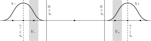
Figure 1. A nontrapped trajectory of the vector field $X_{1}$ with the sets $V_{\pm}$ and the functions $\chi_{\pm}$. The arrows indicate the direction of the field $X=\psi(\rho)X_{1}$.

Proof.

We construct $\chi_{+}$; the function $\chi_{-}$ is constructed similarly, reversing the direction of the flow. By compactness of $V_{+}$, it suffices to prove the lemma for the case when $V_{+}=\{x_{0}\}$, where $x_{0}\in\Sigma_{+}\setminus\mathcal{U}$. Note that $x_{0}\in\{\rho>-\varepsilon\}$ since $x_{0}\in\Sigma_{+}$ and $X$ vanishes on $\{\rho=-\varepsilon\}$.

We first claim that $X_{1}\rho(x_{0})<0$. Indeed, assume that $X_{1}\rho(x_{0})\geq 0$. Then by part 2 of Lemma 2.6 (with $[\alpha,\beta]=[-\varepsilon,0])$, there exists $T\geq 0$ such that $e^{-TX_{1}}(x_{0})\in\{\rho=-\varepsilon\}$ and $e^{-tX_{1}}(x_{0})\notin\mathcal{U}$ for all $t\in[0,T]$. Since $X=\psi(\rho)X_{1}$, we see that $\varphi^{-t}(x_{0})\notin\mathcal{U}$ for all $t\geq 0$, contradicting the fact that $x_{0}\in\Sigma_{+}$.

By part 2 of Lemma 2.6 (with $[\alpha,\beta]=[-\varepsilon,0]$), there exists $T\geq 0$ such that $x_{1}:=e^{TX_{1}}(x_{0})\in\{\rho=-\varepsilon\}$ and $e^{tX_{1}}(x_{0})\in\{-\varepsilon\leq\rho\leq 0\}$, $X_{1}\rho(e^{tX_{1}}(x_{0}))<0$ for all $t\in[0,T]$. Let $U_{1}$ be a small neighborhood of $x_{1}$ in the surface $\{\rho=-\varepsilon\}$. Then for $\delta>0$ small enough, the map

$$(x^{\prime},t)\in U_{1}\times(-T-\delta,\delta)\ \mapsto\ e^{tX_{1}}(x^{\prime})\in\mathcal{M}$$ (2.6)

is a diffeomorphism onto some open subset of $\{-2\varepsilon<\rho<\varepsilon\}\cap\{X_{1}\rho<0\}$. Note that in the $(x^{\prime},t)$ coordinates, $X=\psi(\rho)\partial_{t}$ and $\operatorname{sgn}\psi(\rho)=-\operatorname{sgn}t$. It remains to put in the $(x^{\prime},t)$ coordinates,

$$\chi_{+}(x^{\prime},t)=\chi_{0}(x^{\prime})\chi_{1}(t),$$

where $\chi_{0}\in C_{0}^{\infty}(U_{1};[0,1])$ satisfies $\chi_{0}(x_{1})=1$ and $\chi_{1}\in C_{0}^{\infty}((-T-\delta,\delta);[0,1])$ satisfies $t\chi^{\prime}_{1}(t)\leq 0$ everywhere and $\chi^{\prime}_{1}(-T)>0$. We finally extend $\chi_{+}$ by zero to the entire $\mathcal{M}$. ∎

We finally give the following property of the resolvent $\mathbf{R}(\lambda)$ defined in (1.11).

Lemma 2.9.

Assume that $\psi_{1},\psi_{2}\in C_{0}^{\infty}(\mathcal{U})$ satisfy $\operatorname{supp}\psi_{1}\cap\Gamma_{-}=\operatorname{supp}\psi_{2}\cap\Gamma_{+}=\emptyset$. Then the operators

$$\mathbf{R}(\lambda)\psi_{1},\ \psi_{2}\mathbf{R}(\lambda):C_{0}^{\infty}(\mathcal{U})\to\mathcal{D}^{\prime}(\mathcal{U}),\quad\operatorname{Re}\lambda>C_{0},$$

extend holomorphically to $\lambda\in\mathbb{C}$.

Proof.

We establish holomorphic extension of $\mathbf{R}(\lambda)\psi_{1}$; the extension of $\psi_{2}\mathbf{R}(\lambda)$ is handled similarly. There exists $T>0$ such that $\varphi^{t}(\operatorname{supp}\psi_{1})\cap\mathcal{U}=\emptyset$ for all $t\geq T$. Indeed, it is enough to show this for some $T=T(x_{0})$ when the compact set $\operatorname{supp}\psi_{1}$ is replaced by a small neighborhood $U_{0}$ of some fixed $x_{0}\in\operatorname{supp}\psi_{1}$. Since $x_{0}\notin\Gamma_{-}$, there exists $T>0$ such that $\varphi^{T}(x_{0})\notin\overline{\mathcal{U}}$. It follows that $\varphi^{T}(x)\notin\overline{\mathcal{U}}$ when $x$ lies in a small neighborhood of $U_{0}$ of $x_{0}$. By convexity of $\mathcal{U}$, it follows that $\varphi^{t}(x)\notin\mathcal{U}$ for $t\geq T$ and $x\in U_{0}$.

The holomorphic extension of $\mathbf{R}(\lambda)\psi_{1}$ is now given by the formula

$$\mathbf{R}(\lambda)\psi_{1}\mathbf{f}=\int_{0}^{T}\big{(}e^{-t(\mathbf{X}+\lambda)}\psi_{1}\mathbf{f}\big{)}\big{|}_{\mathcal{U}}\,dt,$$ (2.7)

where we used the fact that $\big{(}e^{-t(\mathbf{X}+\lambda)}\psi_{1}\mathbf{f}\big{)}\big{|}_{\mathcal{U}}=0$ for $t\geq T$, following from (1.8). ∎

2.2. Hyperbolic sets

We next express the assumption (A4) from the introduction in terms of the action of the differential on the dual space. Define the function on the cotangent bundle $T^{*}\mathcal{M}$

$$p(x,\xi)=\langle X(x),\xi\rangle,$$ (2.8)

then its Hamiltonian flow is the action of $d\varphi^{t}$ on covectors:

$$e^{tH_{p}}(x,\xi)=(\varphi^{t}(x),(d\varphi^{t}(x))^{-T}\cdot\xi),\quad x\in\mathcal{M},\ \xi\in T^{*}_{x}\mathcal{M},$$ (2.9)

where $(d\varphi^{t}(x))^{-T}:T^{*}_{x}\mathcal{M}\to T^{*}_{\varphi^{t}(x)}\mathcal{M}$ is the inverse transpose of $d\varphi^{t}(x):T_{x}\mathcal{M}\to T_{\varphi^{t}(x)}\mathcal{M}$. For each $x\in K$, define the dual stable/unstable decomposition

$$T_{x}^{*}\mathcal{M}=E_{0}^{*}(x)\oplus E_{s}^{*}(x)\oplus E_{u}^{*}(x),$$ (2.10)

where $E_{0}^{*}$ is the annihilator of $E_{s}\oplus E_{u}$, $E_{s}^{*}$ is the annihilator of $E_{0}\oplus E_{s}$, and $E_{u}^{*}$ is the annihilator of $E_{0}\oplus E_{u}$. Note the reversal of roles of $E_{s},E_{u}$. By (1.5), we have

$$|(d\varphi^{t}(x))^{-T}\cdot\xi|\leq Ce^{-\gamma|t|}|\xi|,\quad\begin{cases}t\geq 0,\ \xi\in E_{s}^{*}(x);\\ t\leq 0,\ \xi\in E_{u}^{*}(x).\end{cases}$$ (2.11)

We now extend the bundles $E_{s}^{*},E_{u}^{*}$ to $\Gamma_{-},\Gamma_{+}$ respectively, and study the global dynamics of the flow $e^{tH_{p}}$:

Lemma 2.10.

There exist vector subbundles $E^{*}_{\pm}\subset T_{\Gamma_{\pm}}^{*}\mathcal{M}$ over $\Gamma_{\pm}$ such that:

1. $E_{+}^{*}|_{K}=E_{u}^{*}$, $E_{-}^{*}|_{K}=E_{s}^{*}$, and $E_{\pm}^{*}(x)$ depend continuously on $x\in\Gamma_{\pm}$.

2. $E_{\pm}^{*}$ are invariant under the flow $\varphi^{t}$ and $\langle X,\eta\rangle=0$ for $\eta\in E_{\pm}^{*}$.

3. If $x\in\Gamma_{\pm}$ and $\xi\in E_{\pm}^{*}(x)$, then as $t\to\mp\infty$

$$|(d\varphi^{t}(x))^{-T}\xi|\leq\widetilde{C}e^{-\tilde{\gamma}|t|}|\xi|$$ (2.12)

for some constants $\widetilde{C},\tilde{\gamma}>0$ independent of $x,\xi$.

4. If $x\in\Gamma_{\pm}$ and $\xi\in T^{*}_{x}\mathcal{M}$ satisfies $p(x,\xi)=0$ and $\xi\notin E_{\pm}^{*}(x)$, then as $t\to\mp\infty$

$$|(d\varphi^{t}(x))^{-T}\xi|\to\infty,\quad{(d\varphi^{t}(x))^{-T}\xi\over|(d\varphi^{t}(x))^{-T}\xi|}\to E_{\mp}^{*}|_{K}.$$ (2.13)

Proof.

We construct $E_{-}^{*}$; the bundle $E_{+}^{*}$ is contructed similarly. The lemma is a natural consequence of the lamination of $\Gamma_{-}$ by the weak stable manifolds $(W_{s}(x))_{x\in K}$ of the flow, where we put $E_{-}^{*}$ to be the annihilator of the tangent space of $W_{s}(x)$, see for example [NoZw09, §3.3]; the construction of $W_{s}(x)$ ultimately relies on the Hadamard–Perron Theorem [KaHa, Theorem 6.2.8]. However, to make the paper more self-contained and since we only need a small portion of the proof of the Hadamard–Perron theorem, we sketch a direct proof of the lemma below.

We fix some smooth Riemannian metric $\tilde{g}$ on $\mathcal{M}$ and measure the norms of cotangent vectors with respect to this metric. Denote by $d_{\tilde{g}}(\cdot,\cdot)$ the distance function induced by $\tilde{g}$. Take $\varepsilon>0$ small enough to be fixed later; we in particular let $\varepsilon$ be smaller than the injectivity radius of $(\mathcal{M},\tilde{g})$. (This constant is unrelated to the one in Lemma 2.1.) For $x,y\in\mathcal{M}$ such that $d_{\tilde{g}}(x,y)<\varepsilon$, let

$$\tau_{x\to y}:T^{*}_{x}\mathcal{M}\to T^{*}_{y}\mathcal{M}$$

be the parallel transport along the shortest geodesic from $x$ to $y$.

Using (2.11), fix $t_{0}>0$ such that for each $t\geq t_{0}$, $y\in K$ and $\eta\in T^{*}_{y}\mathcal{M}$,

$$|(d\varphi^{t}(y))^{-T}\eta|\leq{1\over 10}|\eta|, \quad\eta\in E_{s}^{*}(y);$$

$$|(d\varphi^{t}(y))^{-T}\eta|\geq 10|\eta|, \quad\eta\in E_{u}^{*}(y).$$

For each $y\in K$, let

$$\pi_{s}(y):T_{y}^{*}\mathcal{M}\to E_{s}^{*}(y),\quad\pi_{u}(y):T_{y}^{*}\mathcal{M}\to E_{u}^{*}(y)$$

be the projection maps corresponding to the decomposition (2.11).

For $x\in\mathcal{M}$, $y\in K$, and $d_{\tilde{g}}(x,y)<\varepsilon$, define the dual stable/unstable cones inside the annihilator of $X$ in $T_{x}^{*}\mathcal{M}$:

$$\begin{gathered}\mathcal{C}^{(y)}_{s}(x)=\{\xi\in T_{x}^{*}\mathcal{M}\mid p(x,\xi)=0,\ |\pi_{s}(y)\tau_{x\to y}\xi|\geq|\pi_{u}(y)\tau_{x\to y}\xi|\},\\ \mathcal{C}^{(y)}_{u}(x)=\{\xi\in T_{x}^{*}\mathcal{M}\mid p(x,\xi)=0,\ |\pi_{u}(y)\tau_{x\to y}\xi|\geq|\pi_{s}(y)\tau_{x\to y}\xi|\}.\end{gathered}$$ (2.14)

Then for $\varepsilon$ small enough and each $t\in[t_{0},2t_{0}]$, $y,y^{\prime}\in K$, and $x\in\mathcal{M}$ such that $d_{\tilde{g}}(x,y)<\varepsilon$, $d_{\tilde{g}}(\varphi^{t}(x),y^{\prime})<\varepsilon$, we have similarly to [KaHa, Lemma 6.2.10]

$$(d\varphi^{t}(x))^{-T}\mathcal{C}^{(y)}_{u}(x) \ \Subset\ \mathcal{C}^{(y^{\prime})}_{u}(\varphi^{t}(x)),$$ (2.15)

$$(d\varphi^{t}(x))^{-T}\mathcal{C}^{(s)}_{s}(x) \ \Supset\ \mathcal{C}^{(y^{\prime})}_{s}(\varphi^{t}(x)).$$

Indeed, (2.15) is verified directly for the case $x=y,\varphi^{t}(x)=y^{\prime}$, and it follows for small $\varepsilon$ by continuity. Moreover, similarly to [KaHa, Lemma 6.2.11] we find for $t\in[t_{0},2t_{0}]$,

$$|(d\varphi^{t}(x))^{-T}\xi|\geq 4|\xi|, \quad\xi\in\mathcal{C}^{(y)}_{u}(x);$$ (2.16)

$$|(d\varphi^{-t}(x))^{-T}\xi|\geq 4|\xi|, \quad\xi\in\mathcal{C}^{(y)}_{s}(x).$$

For $x\in\Gamma_{-}$, we define $E^{*}_{-}(x)$ as follows: $\xi\in T_{x}^{*}\mathcal{M}$ lies in $E^{*}_{-}(x)$ if and only if $p(x,\xi)=0$ and there exists $t_{1}\geq 0$ such that for all $t\geq t_{1}$ and each $y\in K$ such that $d_{\tilde{g}}(\varphi^{t}(x),y)<\varepsilon$, we have $(d\varphi^{t}(x))^{-T}\xi\in\mathcal{C}^{(y)}_{s}(\varphi^{t}(x))$. (Recall that $d_{\tilde{g}}(\varphi^{t}(x),K)\to 0$ as $t\to+\infty$ by Lemma 2.3.)

By a straightforward adaptation of the proof of [KaHa, Proposition 6.2.12], we see that $E^{*}_{-}(x)$ is a linear subbundle of $T^{*}_{\Gamma_{-}}\mathcal{M}$ invariant under $\varphi^{t}$. In fact, for each $t_{j}\to+\infty$ and $y_{j}\in K$ with $d_{\tilde{g}}(\varphi^{t_{j}}(x),y_{j})<\varepsilon$, we have

$$E^{*}_{-}(x)=\lim_{j\to\infty}(d\varphi^{t_{j}}(x))^{T}\tau_{y_{j}\to\varphi^{t_{j}}(x)}E_{s}^{*}(y_{j})$$

where the limit is taken in the Grassmanian of $T_{x}^{*}\mathcal{M}$. The fact that $E^{*}_{-}(x)=E_{s}^{*}(x)$ for $x\in K$ follows from here immediately, as we can take $y_{j}:=\varphi^{t_{j}}(x)$. The bound (2.12) follows directly from (2.16).

To show (2.13), take $x\in\Gamma_{-}$ and $\xi\in T^{*}_{x}\mathcal{M}$ such that $p(x,\xi)=0$ and $\xi\notin E_{-}^{*}(x)$. By Lemma 2.3, there exists $t_{1}\geq 0$ and $y_{1}\in K$ such that $d_{\tilde{g}}(\varphi^{t_{1}}(x),y_{1})<\varepsilon$ and

$$\begin{gathered}d_{\tilde{g}}(\varphi^{t}(x),K)<\varepsilon\quad\text{for }t\geq t_{1};\quad(d\varphi^{t_{1}}(x))^{-T}\xi\notin\mathcal{C}_{s}^{(y_{1})}(\varphi^{t_{1}}(x)).\end{gathered}$$ (2.17)

Iterating (2.15), we see that

$$(d\varphi^{t}(x))^{-T}\xi\in\mathcal{C}_{u}^{(y)}(\varphi^{t}(x)),\quad t\geq t_{0}+t_{1},$$ (2.18)

for each $y\in K$ such that $d_{\tilde{g}}(\varphi^{t}(x),y)<\varepsilon$. Iterating (2.16), we get $|(d\varphi^{t}(x))^{-T}\xi|\to\infty$ as $t\to+\infty$. To see the second part of (2.13), it suffices to take an arbitrary sequence $t_{j}\to+\infty$ such that

$$\varphi^{t_{j}}(x)\to x_{\infty}\in K,\quad{(d\varphi^{t_{j}}(x))^{-T}\xi\over|(d\varphi^{t_{j}}(x))^{-T}\xi|}\to\xi_{\infty}\in T_{x_{\infty}}^{*}\mathcal{M}$$

and prove that $\xi_{\infty}\in E_{u}^{*}(x_{\infty})$. Clearly $p(x_{\infty},\xi_{\infty})=0$. Next, for each $t\geq 0$, we have

$$(d\varphi^{-t}(x_{\infty}))^{-T}\xi_{\infty}=\lim_{j\to\infty}{(d\varphi^{t_{j}-t}(x))^{-T}\xi\over|(d\varphi^{t_{j}}(x))^{-T}\xi|}\in\mathcal{C}_{u}^{(\varphi^{-t}(x_{\infty}))}(\varphi^{-t}(x_{\infty})),$$

which implies that $\xi_{\infty}\in E_{u}^{*}(x_{\infty})$ as needed.

Finally, to show that $E_{-}^{*}(x)$ depends continuously on $x$, note that the condition (2.17) is stable under perturbations of $x,\xi$ (recall that the convergence of Lemma 2.3 is uniform in $x$); on the other hand, similarly to (2.18) the condition (2.17) implies that $\xi\notin E_{-}^{*}(x)$. ∎

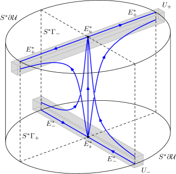
Figure 2. A schematic representation of the flow lines $e^{tH_{p}}$ (thick blue lines) on $S^{*}\mathcal{U}$, which is depicted by the cylinder. The vertical direction in the picture corresponds to the fibers of $S^{*}\mathcal{U}$. The two vertical planes are $S^{*}\Gamma_{\pm}$, containing the subbundles $E_{\pm}^{*}$ (formally speaking, their images under $\kappa$); the vertical line in the middle is $S^{*}K$, containing the subbundles $E_{u}^{*},E_{s}^{*}$. The shaded regions are the neighborhoods $U_{\pm}\supset E_{\pm}^{*}$.

The subbundle $E_{+}^{*}$ is a generalized radial sink and $E_{-}^{*}$ is a generalized radial source in the following sense (this definition is a modification of [DyZw13, (2.12)]).

Lemma 2.11.

Let $\kappa:T^{*}\mathcal{M}\setminus 0\to S^{*}\mathcal{M}$ be the canonical projection, where $S^{*}\mathcal{M}$ is the cosphere bundle over $\mathcal{M}$. Fix open neighborhoods $U_{\pm}\subset S^{*}\mathcal{M}$ of $\kappa(E_{\pm}^{*})$ such that $\overline{U_{\pm}}\cap\kappa(E_{\mp}^{*})=\emptyset$ (see Figure 2). Then for all $(x,\xi)\in T^{*}\mathcal{M}\setminus 0$ such that $p(x,\xi)=0$, $\kappa(x,\xi)\in U_{\pm}$, and $x,\varphi^{t}(x)\in\overline{\mathcal{U}}$, we have

$$d\big{(}\kappa(e^{tH_{p}}(x,\xi)),\kappa(E_{\pm}^{*})\big{)}\to 0 \quad\text{as }t\to\pm\infty;$$ (2.19)

$$|(d\varphi^{t}(x))^{-T}\xi|\geq C^{-1}e^{\tilde{\gamma}|t|}|\xi| \quad\text{for }\pm t\geq 0,$$

uniformly in $(x,\xi)$. Here $d$ denotes any distance function on $S^{*}\mathcal{M}$ and $C,\tilde{\gamma}>0$ are constants independent of $x,\xi$.

Proof.

We study the trajectories starting in $U_{+}$ for $t\geq 0$; the behavior in $U_{-}$ for $t\leq 0$ is proved similarly. It suffices to show that for each sequences $(x_{j},\xi_{j}),(y_{j},\eta_{j})\in T^{*}\mathcal{M}\setminus 0$ and $t_{j}\to+\infty$ such that $e^{t_{j}H_{p}}(x_{j},\xi_{j})=(y_{j},\eta_{j})$, $p(x_{j},\xi_{j})=0$, $\kappa(x_{j},\xi_{j})\in U_{+}$, and $x_{j},y_{j}\in\overline{\mathcal{U}}$, we have

$$d\big{(}\kappa(y_{j},\eta_{j}),\kappa(E_{\pm}^{*})\big{)}\to 0,\quad|\eta_{j}|\geq C^{-1}e^{\tilde{\gamma}t_{j}}|\xi_{j}|.$$ (2.20)

By passing to a subsequence, we may assume that $x_{j}\to x_{\infty}\in\overline{\mathcal{U}}$, $y_{j}\to y_{\infty}\in\overline{\mathcal{U}}$. For each $t\geq 0$, $\varphi^{t}(x_{\infty})=\lim_{j\to\infty}\varphi^{t}(x_{j})\in\mathcal{\overline{U}}$, therefore $x_{\infty}\in\Gamma_{-}$. Similarly $y_{\infty}\in\Gamma_{+}$. We also pass to a subsequence to make $\xi_{j}/|\xi_{j}|\to\xi_{\infty}\in T^{*}_{x_{\infty}}\mathcal{M}$, $\eta_{j}/|\eta_{j}|\to\eta_{\infty}\in T^{*}_{y_{\infty}}\mathcal{M}$, with $|\xi_{\infty}|=|\eta_{\infty}|=1$. Since $\kappa(x_{j},\xi_{j})\in U_{+}$ and $\overline{U_{+}}$ does not intersect $\kappa(E_{-}^{*})$, we have $\xi_{\infty}\notin E_{-}^{*}(x_{\infty})$.

For the first part of (2.20), we need to prove that $\eta_{\infty}\in E_{+}^{*}(y_{\infty})$. Assume the contrary. We will use the proof of Lemma 2.10. Similarly to (2.18), for $t_{2}>0$ large enough and each $x^{\prime},y^{\prime}\in K$ such that $d_{\tilde{g}}(\varphi^{t_{2}}(x_{\infty}),x^{\prime}),d_{\tilde{g}}(\varphi^{-t_{2}}(y_{\infty}),y^{\prime})<\varepsilon$, we have

$$(d\varphi^{t_{2}}(x_{\infty}))^{-T}\xi_{\infty}\notin\mathcal{C}^{(x^{\prime})}_{s}(\varphi^{t_{2}}(x_{\infty})),\quad(d\varphi^{-t_{2}}(y_{\infty}))^{-T}\eta_{\infty}\notin\mathcal{C}^{(y^{\prime})}_{u}(\varphi^{-t_{2}}(y_{\infty})).$$

It follows that for $t_{2}$ large and fixed, and $j$ large enough depending on $t_{2}$, we have

$$(d\varphi^{t_{2}}(x_{j}))^{-T}\xi_{j}\notin\mathcal{C}^{(x^{\prime})}_{s}(\varphi^{t_{2}}(x_{j})),\quad(d\varphi^{-t_{2}}(y_{j}))^{-T}\eta_{j}\notin\mathcal{C}^{(y^{\prime})}_{u}(\varphi^{-t_{2}}(y_{j})),$$ (2.21)

for each $x^{\prime},y^{\prime}\in K$ such that $d_{\tilde{g}}(\varphi^{t_{2}}(x_{j}),x^{\prime}),d_{\tilde{g}}(\varphi^{-t_{2}}(y_{j}),y^{\prime})<\varepsilon$. By Lemma 2.4, we can furthermore fix $t_{2}$ large enough so that for $t_{j}\geq 2t_{2}$, $d_{\tilde{g}}(\varphi^{t}(x_{j}),K)<\varepsilon$ for $t\in[t_{2},t_{j}-t_{2}]$. Now, by the first statement of (2.21) and iterating (2.15), for $j$ large enough and $x^{\prime}\in K,d_{\tilde{g}}(x^{\prime},\varphi^{t_{j}/2}(x_{j}))<\varepsilon$, we have $(d\varphi^{t_{j}/2}(x_{j}))^{-T}\xi_{j}\notin\mathcal{C}^{(x^{\prime})}_{s}(\varphi^{t_{j}/2}(x_{j}))$. Similarly from the second statement of (2.21) we get $(d\varphi^{-t_{j}/2}(y_{j}))^{-T}\eta_{j}\notin\mathcal{C}^{(y^{\prime})}_{u}(\varphi^{-t_{j}/2}(y_{j}))$. However, these two vectors are the same, giving a contradiction and implying the first part of (2.20).

The proof of the second part of (2.20) works in a similar fashion, using (2.16). ∎

To construct the weight function for anisotropic Sobolev spaces, we need the following adaptation of [FaSj, Lemma 2.1] (see also [DyZw13, Lemma C.1]). We consider $e^{tH_{p}}$ as a flow on the sphere bundle $S^{*}\mathcal{M}$, by pulling it back by the projection $\kappa:T^{*}\mathcal{M}\setminus 0\to S^{*}\mathcal{M}$. Consider also the projection $\pi:S^{*}\mathcal{M}\to\mathcal{M}$.

Lemma 2.12.

Let $U_{\pm}\subset S^{*}\mathcal{M}$ be the neighborhoods of $\kappa(E_{\pm}^{*})$ introduced in Lemma 2.11. Then there exist functions $m_{\pm}\in C^{\infty}(S^{*}\mathcal{M})$ such that:

1. $m_{\pm}=1$ near $\kappa(E_{\pm}^{*})$ and $0\leq m_{\pm}\leq 1$ everywhere;

2. $\operatorname{supp}m_{\pm}\cap\{p=0\}\cap\pi^{-1}(\overline{\mathcal{U}})\ \subset\ U_{\pm}$;

3. $\operatorname{supp}m_{\pm}\subset\pi^{-1}(\Sigma_{\pm})$, where $\Sigma_{\pm}$ is defined in (2.4);

4. $\pm H_{p}m_{\pm}\geq 0$ on $V\cap\pi^{-1}(\mathcal{U})$, where $V$ is a neighborhood of $\{p=0\}$.

Proof.

We construct $m_{+}$; the function $m_{-}$ is constructed similarly, reversing the direction of propagation. Let $W\Subset\mathcal{U}$ be an open neighborhood of $K$. Fix $m_{0}\in C_{0}^{\infty}(U_{+}\cap\pi^{-1}(\mathcal{U}))$ such that $m_{0}=1$ in a neighborhood of $\kappa(E_{+}^{*})\cap\pi^{-1}(\overline{W})$ and $0\leq m_{0}\leq 1$ everywhere.

We show that for $T>0$ large enough and fixed, the function

$$m_{+}(x,\xi)={1\over T}\int_{T}^{2T}m_{0}(e^{-tH_{p}}(x,\xi))\,dt$$

has the required properties:

1. Clearly $0\leq m_{+}\leq 1$ everywhere. Now, take $(x,\xi)\in\kappa(E_{+}^{*})$. Then $x\in\Gamma_{+}$. By Lemma 2.3, $\varphi^{-t}(x)\in W$ for all $t\in[T,2T]$ and $T$ large enough. Since $E_{+}^{*}$ is invariant under the flow, we have $e^{-tH_{p}}(x,\xi)\in\kappa(E_{+}^{*})$ and thus $m_{0}(e^{-tH_{p}}(x,\xi))=1$ for $t\in[T,2T]$, implying that $m(x,\xi)=1$. Same argument works when $(x,\xi)$ lies in a small neighborhood of $\kappa(E_{+}^{*})$.

2. Assume that $(x,\xi)\in\operatorname{supp}m_{+}\cap\{p=0\}\cap\pi^{-1}(\overline{\mathcal{U}})$. Then there exists $t\in[T,2T]$ such that $e^{-tH_{p}}(x,\xi)\in\operatorname{supp}m_{0}$. Note that $x,\varphi^{-t}(x)\in\overline{\mathcal{U}}$ and $e^{-tH_{p}}(x,\xi)\in U_{+}$. Then by Lemma 2.11, for $T$ large enough and $t\in[T,2T]$, we have $(x,\xi)\in U_{+}$ as required.

3. This follows immediately from (2.4) and the fact that $\operatorname{supp}m_{0}\subset\pi^{-1}(\mathcal{U})$.

4. Assume that $(x,\xi)\in S^{*}\mathcal{M}$, $x\in\mathcal{U}$, and $p(x,\xi)=0$. Then

   $$H_{p}m_{+}(x,\xi)={1\over T}\big{(}m_{0}(e^{-TH_{p}}(x,\xi))-m_{0}(e^{-2TH_{p}}(x,\xi))\big{)}.$$

   We then need to show that $m_{0}(e^{-TH_{p}}(x,\xi))\geq m_{0}(e^{-2TH_{p}}(x,\xi))$. Since $0\leq m_{0}\leq 1$, we only need to handle the case when $m_{0}(e^{-TH_{p}}(x,\xi))<1$ and $m_{0}(e^{-2TH_{p}}(x,\xi))>0$. In particular, we have $\varphi^{-2T}(x)\in\mathcal{U}$, and by Lemma 2.4, for $T$ large enough, we have $\varphi^{-T}(x)\in W$. Then $e^{-TH_{p}}(x,\xi)$ does not lie in some fixed neighborhood $W_{1}$ of $\kappa(E_{+}^{*})$, depending only on $m_{0}$. On the other hand, $e^{-2TH_{p}}(x,\xi)\in U_{+}$ and $\varphi^{-2T}(x),\varphi^{-T}(x)\in\overline{\mathcal{U}}$. By Lemma 2.11, we reach a contradiction for $T$ large enough. Same reasoning applies if we replace the condition $p(x,\xi)=0$ by $(x,\xi)\in V$ for some neighborhood $V$ of $\{p=0\}$. ∎

2.3. Estimates on recurrence

We finally give an extension of the recurrence estimates [DyZw13, Appendix A] to our situation, used in §5.1. Throughout this subsection, we fix $t_{e}>0$ and a compact subset $V\subset\mathcal{U}$. We also consider the distance function $d_{\tilde{g}}$ and the parallel transport operators $\tau_{x\to y}$ introduced in the proof of Lemma 2.10, defined for $d_{\tilde{g}}(x,y)<\varepsilon$, where $\varepsilon>0$ is a small constant (unrelated to the constant in Lemma 2.1). We however ask that $\tau_{x\to y}$ act on the tangent spaces $T_{x}\mathcal{M}\to T_{y}\mathcal{M}$ instead of the cotangent spaces. We start with

Lemma 2.13.

For each $\varepsilon_{1}>0$, there exists $\delta_{1}>0$ such that

$$d_{\tilde{g}}(x,\varphi^{t}(x))<\delta_{1},\ t\geq t_{e},\ x\in V\ \Longrightarrow\ d_{\tilde{g}}(x,K)<\varepsilon_{1}.$$

Proof.

It suffices to show that for each sequences $x_{j}\in V$, $t_{j}\geq t_{0}$ such that $x_{j}\to x_{\infty}\in\mathcal{U}$ and $d(x_{j},\varphi^{t_{j}}(x_{j}))\to 0$, we have $x_{\infty}\in K$. We have $\varphi^{t_{j}}(x_{j})\to x_{\infty}$. By passing to a subsequence we may assume that $t_{j}\to t_{\infty}\in(0,\infty]$. If $t_{\infty}<\infty$, then $\varphi^{t_{\infty}}(x_{\infty})=x_{\infty}$ and thus $x_{\infty}\in K$. Assume now that $t_{\infty}=\infty$. For each $t\geq 0$ and $j$ large enough depending on $t$, we have $t_{j}\geq t$ and $x_{j},\varphi^{t_{j}}(x_{j})\in\mathcal{U}$; by (1.2), $\varphi^{t}(x_{j})\in\mathcal{U}$ and $\varphi^{t_{j}-t}(x_{j})\in\mathcal{U}$. Passing to the limit, we see that $\varphi^{t}(x_{\infty})$ and $\varphi^{-t}(x_{\infty})$ lie in $\overline{\mathcal{U}}$; since $t$ was chosen arbitrarily, we get $x_{\infty}\in K$. ∎

Denote by $\pi^{\perp}:T\mathcal{U}\to T\mathcal{U}$ the orthogonal projection onto the orthogonal complement of $E_{0}=\mathbb{R}X$ (with respect to some fixed Riemannian metric). This operator need not be invariant under $d\varphi^{t}$ and its image need not be equal to $E_{u}\oplus E_{s}$. However, there exists a constant $C>0$ such that for each $x\in K$ and $v=v_{0}+v_{u}+v_{s}\in T_{x}\mathcal{M}$, $v_{0}\in E_{0}(x)$, $v_{u}\in E_{u}(x)$, $v_{s}\in E_{s}(x)$,

$$C^{-1}(|v_{u}|+|v_{s}|)\leq|\pi^{\perp}(v)|\leq C(|v_{u}|+|v_{s}|).$$ (2.22)

Moreover, $\pi^{\perp}(d\varphi^{t}(x)\cdot v)$ depends only on $\pi^{\perp}(v)$:

$$\pi^{\perp}(d\varphi^{t}(x)\cdot v)=\pi^{\perp}(d\varphi^{t}(x)\cdot\pi^{\perp}(v))$$ (2.23)

The next lemma gives a convexity property for the absolute value of a vector propagated along the flow.

Lemma 2.14.

There exists $T_{0}>0$ such that for each $t\geq T_{0}$, $\varepsilon_{t}>0$ small enough depending on $t$, and each $(x,v)\in T\mathcal{U}$ with $d_{\tilde{g}}(x,K)<\varepsilon_{t}$,

$$|\pi^{\perp}(v)| \leq{|\pi^{\perp}(d\varphi^{t}(x)\cdot v)|+|\pi^{\perp}(d\varphi^{-t}(x)\cdot v)|\over 4}.$$ (2.24)

Proof.

Assume first that $x\in K$. Then $v=v_{0}+v_{u}+v_{s}$, where $v_{0}\in E_{0}(x),v_{u}\in E_{u}(x),v_{s}\in E_{s}(x)$. By (1.5), there exists a constant $C$ such that for all $t\geq T_{0}$,

$$|v_{u}|\leq Ce^{-\gamma T_{0}}|d\varphi^{t}(x)\cdot v_{u}|,\quad|v_{s}|\leq Ce^{-\gamma T_{0}}|d\varphi^{-t}(x)\cdot v_{s}|,\quad$$

Adding these up and using (2.22), we get for some other constant $C$,

$$|\pi^{\perp}(v)|\leq Ce^{-\gamma T_{0}}(|\pi^{\perp}(d\varphi^{t}(x)\cdot v)|+|\pi^{\perp}(d\varphi^{-t}(x)\cdot v)|).$$

It remains to take $T_{0}$ large enough. The case of $x$ with $d_{\tilde{g}}(x,K)<\varepsilon_{t}$ follows by continuity. ∎

The following is a generalization of [DyZw13, Lemma A.1]:

Lemma 2.15.

There exist $\delta>0$ and $C$ such that for each $x\in V,t\geq t_{e},v\in T_{x}\mathcal{M}$ satisfying $d_{\tilde{g}}(x,\varphi^{t}(x))<\delta$ and $v\perp X(x)$,

$$|v|+|w|\leq C|\pi^{\perp}(w)|,\quad w:=(d\varphi^{t}(x)-\tau_{x\to\varphi^{t}(x)})v.$$

Proof.

It suffices to show that for each sequences

$$x_{j}\in V,\quad t_{j}\geq t_{e},\quad v_{j}\perp X(x_{j}),\quad w_{j}:=(d\varphi^{t_{j}}(x_{j})-\tau_{x_{j}\to\varphi^{t_{j}}(x_{j})})v_{j}$$

such that

$$d_{\tilde{g}}(x_{j},\varphi^{t_{j}}(x_{j}))\to 0,\quad\pi^{\perp}(w_{j})\to 0,$$

we have $v_{j}\to 0$ and $w_{j}\to 0$. By passing to a subsequence and using Lemma 2.13, we may assume that

$$x_{j}\to x_{\infty}\in K,\quad\varphi^{t_{j}}(x_{j})\to x_{\infty},\quad t_{j}\to t_{\infty}\in(0,\infty].$$

Assume first that $t_{\infty}<\infty$. By passing to a subsequence, we may assume that $v_{j}/|v_{j}|\to v_{\infty}\perp X(x_{\infty})$. We have $\varphi^{t_{\infty}}(x_{\infty})=x_{\infty}$ and $w_{j}/|v_{j}|\to d\varphi^{t_{\infty}}(x_{\infty})\cdot v_{\infty}-v_{\infty}$. By (1.5), $\pi^{\perp}(w_{j})/|v_{j}|$ has a nonzero limit; since $\pi^{\perp}(w_{j})\to 0$, we get $v_{j}\to 0$ and thus $w_{j}\to 0$.

We henceforth assume that $t_{\infty}=\infty$. We first show that $v_{j}\to 0$. Assume the contrary, then by passing to a subsequence and rescaling, we can make

$$v_{j}\to v_{\infty}\perp X(x_{\infty}),\quad|v_{\infty}|=1.$$

Consider the following two cases:

Case 1: $v_{\infty}$ has a nonzero $E_{u}$ component in the decomposition (1.4). By (1.5), we have $|\pi^{\perp}(d\varphi^{t}(x_{\infty})\cdot v_{\infty})|\to\infty$ as $t\to+\infty$. Let $T_{0}$ be the constant from Lemma 2.14. Fix $T\geq T_{0}$ so that $|\pi^{\perp}(d\varphi^{T}(x_{\infty})\cdot v_{\infty})|>2$. For $j$ large enough, we have

$$|\pi^{\perp}(d\varphi^{T}(x_{j})\cdot v_{j})|\geq 2|v_{j}|.$$ (2.25)

Moreover, if $\varepsilon_{T}$ is chosen in Lemma 2.14, then for $j$ large enough,

$$d_{\tilde{g}}(e^{tH_{p}}(x_{j}),K)<\varepsilon_{T}\quad\text{for all }t\in[0,t_{j}].$$ (2.26)

Indeed, for $t\in[T^{\prime},t_{j}-T^{\prime}]$ and $T^{\prime}$ large enough depending on $\varepsilon_{T}$, this follows from Lemma 2.4; for other values of $t$, it follows from continuity and the fact that both $x_{j}$ and $\varphi^{t_{j}}(x_{j})$ converge to $x_{\infty}\in K$.

We have for each $\ell\in\mathbb{N}_{0}$ such that $\ell T\leq t_{j}$,

$$|\pi^{\perp}(d\varphi^{(\ell+1)T}(x_{j})\cdot v_{j})|\geq 2|\pi^{\perp}(d\varphi^{\ell T}(x_{j})\cdot v_{j})|.$$

This is proved by induction on $\ell$; the base $\ell=0$ of the induction is given by (2.25) and the inductive step follows from (2.24) applied to $v=d\varphi^{\ell T}(x_{j})\cdot v_{j}$, $t=T$. We can modify $T$ a tiny bit depending on $j$ so that $t_{j}/T$ is an integer; then we obtain

$$|\pi^{\perp}(d\varphi^{t_{j}}(x_{j})\cdot v_{j})|\geq 2^{t_{j}/T}|v_{j}|.$$

This implies that $|\pi^{\perp}(w_{j})|\to\infty$, a contradiction.

Case 2: $v_{\infty}$ has a nonzero $E_{s}$ component in the decomposition (1.4). Since $\pi^{\perp}(w_{j})\to 0$, we have $\pi^{\perp}(d\varphi^{t_{j}}(x_{j})\cdot v_{j})\to v_{\infty}$. Arguing as in case (i), with $\varphi^{t_{j}}(x_{j}),d\varphi^{t_{j}}(x_{j})\cdot v_{j}$ replacing $x_{j},v_{j}$, and going backwards along the flow, we get

$$|\pi^{\perp}(d\varphi^{t_{j}-(\ell+1)T}(x_{j})\cdot v_{j})|\geq 2|\pi^{\perp}(d\varphi^{t_{j}-\ell T}(x_{j})\cdot v_{j})|$$

which implies

$$|\pi^{\perp}(d\varphi^{t_{j}}(x_{j})\cdot v_{j})|\leq 2^{-t_{j}/T}|v_{j}|.$$

Then $\pi^{\perp}(w_{j})\to-v_{\infty}$, a contradiction.

We now show that $w_{j}\to 0$. Let $T_{0}$ be the constant from Lemma 2.14 and fix $T>T_{0}$; we will modify it a little bit depending on $j$ so that $L:=t_{j}/T$ is an integer. For large $j$, (2.26) is satisfied. For each $v\in T\mathcal{U}$, define $\pi_{0}(v)\in\mathbb{R}$ by the formula

$$v=\pi^{\perp}(v)+\pi_{0}(v)X.$$

Since $X$ is invariant under the flow, we have for some constant $C$,

$$|\pi_{0}(d\varphi^{(\ell+1)T}(x_{j})\cdot v_{j})-\pi_{0}(d\varphi^{\ell T}(x_{j})\cdot v_{j})|\leq C|\pi^{\perp}(d\varphi^{\ell T}(x_{j})\cdot v_{j})|.$$

Summing these up and using that $\pi_{0}(v_{j})=0$, we get

$$|\pi_{0}(d\varphi^{t_{j}}(x_{j})\cdot v_{j})|\leq C\sum_{\ell=0}^{L}|\pi^{\perp}(d\varphi^{\ell T}(x_{j})\cdot v_{j})|.$$

Denote the sum on the right-hand side by $\Sigma$. Using (2.24) for $v=d\varphi^{\ell T}(x_{j})\cdot v_{j}$ and all $\ell=1,\dots,L-1$, we get

$$\Sigma\leq|\pi^{\perp}(v_{j})|+|\pi^{\perp}(d\varphi^{t_{j}}(x_{j})\cdot v_{j})|+\Sigma/2.$$

Since $\pi^{\perp}(w_{j})\to 0$ and $v_{j}\to 0$, we know that $|\pi^{\perp}(v_{j})|+|\pi^{\perp}(d\varphi^{t_{j}}(x_{j})\cdot v_{j})|\to 0$ and thus $\Sigma\to 0$. Then $\pi_{0}(d\varphi^{t_{j}}(x_{j})\cdot v_{j})\to 0$, which implies that $w_{j}\to 0$, as required. ∎

Arguing as in [DyZw13, Appendix A], we obtain from Lemma 2.15 the following analog of [DyZw13, Lemma 2.1]:

Lemma 2.16.

Define the following measure on $\mathcal{M}\times\mathbb{R}$: $\tilde{\mu}=\mu\times dt$, where $\mu$ is some smooth measure on $\mathcal{M}$. Fix $t_{e}>0$ and a compact subset $V\subset\mathcal{U}$. Then there exist constants $C,L$ such that for each $\varepsilon>0$, $T>t_{e}$, and $n=\dim\mathcal{M}$,

$$\tilde{\mu}(\{(x,t)\mid t_{e}\leq t\leq T,\ d(x,\varphi^{t}(x))<\varepsilon,\ x\in V\})\leq C\varepsilon^{n}e^{nLT}.$$

Letting $\varepsilon\to 0$, we obtain the following analog of [DyZw13, Lemma 2.2]:

Lemma 2.17.

Let $N(T)$ be the number of closed trajectories of $\varphi^{t}$ on $K$ of period no more than $T$. Then

$$N(T)\leq Ce^{(2n-1)LT}.$$

3. Semiclassical preliminaries

In this section, we discuss some general results from microlocal and semiclassical analysis, following the notation of [DyZw13, Section 2.3 and Appendix C]. While some of the facts mentioned here (such as Lemma 3.2) are standard, Lemma 3.7 below seems to be a new result.

3.1. Review of semiclassical notation

Recall that we are working on a compact manifold $\mathcal{M}$ without boundary. We use the class $\Psi^{k}(\mathcal{M};\mathcal{E})$ of pseudodifferential operators of order $k$ acting on sections of $\mathcal{E}$. The corresponding symbol class is denoted by $S^{k}(\mathcal{M})$, see [DyZw13, (C.1)]. The principal symbol

$$\sigma(\mathbf{A})\in S^{k}(\mathcal{M};\operatorname{End}(\mathcal{E}))/S^{k-1}(\mathcal{M};\operatorname{End}(\mathcal{E}))$$

of $\mathbf{A}\in\Psi^{k}(\mathcal{M};\mathcal{E})$ is in general a section of the endomorphism bundle $\operatorname{End}(\mathcal{E})$ pulled back to $T^{*}\mathcal{M}$, however in this paper we mostly work with principally scalar operators, whose principal symbols are products of functions on $T^{*}\mathcal{M}$ and the identity homomorphism on $\mathcal{E}$. The wavefront set $\operatorname{WF}(A)$ is a closed conic subset of $T^{*}\mathcal{M}\setminus 0$ which measures the concentration of $A$ in the phase space, and the elliptic set $\operatorname{ell}(A)$ is an open conic subset of $T^{*}\mathcal{M}\setminus 0$ which measures where the principal symbol of $A$ is invertible.

We also use the class of semiclassical pseudodifferential operators $\Psi^{k}_{h}(\mathcal{M};\mathcal{E})$, which depend on a positive parameter $h$ tending to zero. Quantizing a symbol $a(x,\xi)$ in the $h$-sense is equivalent to quantizing the rescaled symbol $a(x,h\xi)$ in the nonsemiclassical sense. We use the notion of the semiclassical principal symbol

$$\sigma_{h}(A)\in S^{k}(\mathcal{M})/hS^{k-1}(\mathcal{M})$$

of a principally scalar $A\in\Psi^{k}_{h}(\mathcal{M};\mathcal{E})$. We also use the fiber-radially compactified cotangent bundle $\overline{T}^{*}\mathcal{M}$; the interior of this bundle is diffeomorphic to $T^{*}\mathcal{M}$ and the boundary $\partial\overline{T}^{*}\mathcal{M}$, called the fiber infinity, is diffeomorphic to the cosphere bundle $S^{*}\mathcal{M}$. The $h$-wavefront set $\operatorname{WF}_{h}(A)$ and the $h$-elliptic set $\operatorname{ell}_{h}(A)$ are now subsets of $\overline{T}^{*}\mathcal{M}$. We use the symbol $\Psi^{\operatorname{comp}}_{h}$ to denote the class of operators in $\Psi^{k}_{h}$ whose wavefront sets are compactly contained in $T^{*}\mathcal{M}$ (that is, do not intersect the fiber infinity).

We use the concept of the wavefront set $\operatorname{WF}(u)\subset T^{*}\mathcal{M}\setminus 0$ of any distribution $u\in\mathcal{D}^{\prime}(\mathcal{M})$. We also consider wavefront sets $\operatorname{WF}^{\prime}(B)\subset T^{*}(\mathcal{M}\times\mathcal{M})\setminus 0$ of operators $B:C^{\infty}(\mathcal{M})\to\mathcal{D}^{\prime}(\mathcal{M})$, defined as follows:

$$\operatorname{WF}^{\prime}(B)=\{(x,\xi,y,-\eta)\mid(x,\xi,y,\eta)\in\operatorname{WF}(K_{B})\}$$ (3.1)

where the Schwartz kernel $K_{B}\in\mathcal{D}^{\prime}(\mathcal{M}\times\mathcal{M})$ is given by the formula (where we use any smooth density $dy$ on $\mathcal{M}$)

$$Bf(x)=\int_{\mathcal{M}}K_{B}(x,y)f(y)\,dy,\quad f\in C^{\infty}(\mathcal{M}).$$ (3.2)

For distributions $u=u(h)$ and operators $B=B(h)$ which are $h$-tempered (in the sense that $\|u(h)\|_{H^{-N}_{h}}=\mathcal{O}(h^{-N})$ for some $N$), we consider the semiclassical wavefront sets $\operatorname{WF}_{h}(u)\subset\overline{T}^{*}\mathcal{M}$, $\operatorname{WF}_{h}^{\prime}(B)\subset\overline{T}^{*}(\mathcal{M}\times\mathcal{M})$. By taking the union of the wavefront sets of all components, we can extend these notions to distributions and operators valued in smooth vector bundles.

We will use the following multiplicative property of $h$-wavefront sets away from fiber infinity: assume that $A(h),B(h):C^{\infty}(\mathcal{M})\to\mathcal{D}^{\prime}(\mathcal{M})$ are $h$-tempered and $Q\in\Psi^{\operatorname{comp}}_{h}(\mathcal{M})$. Using [DyZw13, Lemma 2.3], we obtain

$$\begin{gathered}(x,\xi,z,\zeta)\in\operatorname{WF}_{h}(AQB)\cap T^{*}(\mathcal{M}\times\mathcal{M})\\ \Longrightarrow\ \exists(y,\eta)\in\operatorname{WF}_{h}(Q):(x,\xi,y,\eta)\in\operatorname{WF}_{h}(A),\ (y,\eta,z,\zeta)\in\operatorname{WF}_{h}(B).\end{gathered}$$ (3.3)

Finally, if $u\in\mathcal{D}^{\prime}(\mathcal{V})$, where $\mathcal{V}\subset\mathcal{M}$ is an open set, then $\operatorname{WF}(u)\subset T^{*}\mathcal{V}\setminus 0$ is defined as the union of all $\operatorname{WF}(\chi u)$ for $\chi\in C_{0}^{\infty}(\mathcal{V})$; here $\chi u$ is naturally embedded into $\mathcal{D}^{\prime}(\mathcal{M})$. Similarly one can define $\operatorname{WF}(B)\subset T^{*}(\mathcal{U}\times\mathcal{U})\setminus 0$, where $B:C_{0}^{\infty}(\mathcal{U})\to\mathcal{D}^{\prime}(\mathcal{U})$ and $\mathcal{U}\subset\mathcal{M}$ is open, by using (3.1) and the previous definition with $\mathcal{V}:=\mathcal{U}\times\mathcal{U}$.

3.2. Semiclassical propagation estimates

We start with several semiclassical estimates which form the basis of our proofs. To simplify their statements, we say for $p\in C^{\infty}(T^{*}\mathcal{M})$ that

$$p\in\operatorname{Hom}^{k}(T^{*}\mathcal{M};\mathbb{R})$$

if $p$ is real-valued and homogeneous of degree $k$ in $\xi$ for $|\xi|$ large enough. If $p\in\operatorname{Hom}^{1}(T^{*}\mathcal{M};\mathbb{R})$, then the Hamiltonian field $H_{p}$ extends to a smooth vector field on $\overline{T}^{*}\mathcal{M}$ which is tangent to $\partial\overline{T}^{*}\mathcal{M}$. For later use in this section, we recall the notation

$$\operatorname{Re}\mathbf{A}:={\mathbf{A}+\mathbf{A}^{*}\over 2},\quad\operatorname{Im}\mathbf{A}:={\mathbf{A}-\mathbf{A}^{*}\over 2i},$$

where $\mathbf{A}$ is an operator $C^{\infty}(\mathcal{M};\mathcal{E})\to\mathcal{D}^{\prime}(\mathcal{M};\mathcal{E})$ and we fix a volume form on $\mathcal{M}$ and an inner product on $\mathcal{E}$ to define the adjoint operator $\mathbf{A}^{*}$.

First of all, we review the classical Duistermaat–Hörmander propagation of singularities, formulated using the following

Definition 3.1.

Assume that $p\in\operatorname{Hom}^{1}(T^{*}\mathcal{M};\mathbb{R})$. Let $V,W\subset\overline{T}^{*}\mathcal{M}$ be open sets. We say that a point $(x,\xi)\in\overline{T}^{*}M$ is controlled by $V$ inside of $W$, if there exists $T\geq 0$ such that $e^{-TH_{p}}(x,\xi)\in V$ and $e^{-tH_{p}}(x,\xi)\in W$ for $t\in[0,T]$. Denote by

$$\operatorname{Con}_{p}(V;W)\subset\overline{T}^{*}\mathcal{M}$$ (3.4)

the set of all such points. Note that $\operatorname{Con}_{p}(V;W)$ is an open subset of $\overline{T}^{*}\mathcal{M}$.

Propagation of singularities (see for instance [DyZw13, Proposition 2.5]) is then formulated as follows:

Lemma 3.2.

Assume that $\mathbf{P}\in\Psi^{1}_{h}(\mathcal{M};\mathcal{E})$ is principally scalar and $\sigma_{h}(\mathbf{P})=p-iq$ where $p\in\operatorname{Hom}^{1}(T^{*}\mathcal{M};\mathbb{R})$ and $q$ is real-valued. Let $A,B,B_{1}\in\Psi^{0}_{h}(\mathcal{M})$ be such that

$$q\geq 0\quad\text{near }\operatorname{WF}_{h}(B_{1}),\quad\operatorname{WF}_{h}(A)\subset\operatorname{Con}_{p}(\operatorname{ell}_{h}(B);\operatorname{ell}_{h}(B_{1})).$$

Then for each $s,N$ and $\mathbf{u}\in C^{\infty}(\mathcal{M};\mathcal{E})$, we have

$$\|A\mathbf{u}\|_{H^{s}_{h}}\leq C\|B\mathbf{u}\|_{H^{s}_{h}}+Ch^{-1}\|B_{1}\mathbf{P}\mathbf{u}\|_{H^{s}_{h}}+\mathcal{O}(h^{\infty})\|\mathbf{u}\|_{H^{-N}_{h}}.$$ (3.5)

In this subsection, we give a more general propagation estimate (Lemma 3.7) under the weaker assumption that the trajectories of $e^{-tH_{p}}$ starting on $\operatorname{WF}_{h}(A)$ either pass through $\operatorname{ell}_{h}(B)$ or converge to some closed set $L$, while staying in $\operatorname{ell}_{h}(B_{1})$. This follows a long tradition of study of operators with radial invariant sets, see in particular Guillemin–Schaeffer [GuSc], Melrose [Me], Herbst–Skibsted [HeSk], and Hassell–Melrose–Vasy [HMV]. For the estimate, we need to additionally restrict the sign of the imaginary part of the subprincipal symbol of $\mathbf{P}$ on $L$, which is achieved by the following

Definition 3.3.

Let $\mathbf{P}\in\Psi^{1}_{h}(\mathcal{M};\mathcal{E})$ and $L\subset\overline{T}^{*}\mathcal{M}$ be a closed set. Fix a volume form on $\mathcal{M}$ and an inner product on the fibers of $\mathcal{E}$; this defines an inner product on $L^{2}(\mathcal{M};\mathcal{E})$. Fix also $s\in\mathbb{R}$. We say that

$$\operatorname{Im}\mathbf{P}\lesssim-h\quad\text{on }H^{s}_{h}\quad\text{microlocally near }L$$ (3.6)

if there exist operators

$$\begin{gathered}\mathbf{Y}_{1}\in\Psi^{s}_{h}(\mathcal{M};\mathcal{E}),\quad\mathbf{Y}_{2}\in\Psi^{-s}_{h}(\mathcal{M};\mathcal{E}),\quad\mathbf{Z}\in\Psi^{0}_{h}(\mathcal{M};\mathcal{E});\\ \mathbf{Y}_{1}\mathbf{Y}_{2}=1+\mathcal{O}(h^{\infty})\quad\text{near }L,\quad L\subset\operatorname{ell}_{h}(\mathbf{Z}),\end{gathered}$$

such that for each $N$, $h$ small enough, and each $\mathbf{u}\in H^{1/2}_{h}(\mathcal{M};\mathcal{E})$,

$$\operatorname{Im}\langle\mathbf{Y}_{1}\mathbf{P}\mathbf{Y}_{2}\mathbf{u},\mathbf{u}\rangle_{L^{2}}\leq-h\|\mathbf{Z}\mathbf{u}\|^{2}_{L^{2}}+\mathcal{O}(h^{\infty})\|\mathbf{u}\|_{H^{-N}_{h}}^{2}.$$ (3.7)

Remarks. (i) The above definition does not actually depend on the choice of the volume form on $M$ and the metric on the fibers of $\mathcal{E}$. Indeed, any other choice yields the inner product $\langle\mathbf{u},\mathbf{v}\rangle^{\prime}=\langle\mathbf{W}\mathbf{u},\mathbf{W}\mathbf{v}\rangle$ for some invertible $\mathbf{W}\in C^{\infty}(\mathcal{M};\operatorname{End}(\mathcal{E}))$. Applying (3.7) for the inner product $\langle\cdot,\cdot\rangle$ to $\mathbf{W}\mathbf{u}$, we obtain (3.7) for $\langle\cdot,\cdot\rangle^{\prime}$ with the operators $\mathbf{Y}_{1}^{\prime}=\mathbf{W}^{-1}\mathbf{Y}_{1}$, $\mathbf{Y}_{2}^{\prime}=\mathbf{Y}_{2}\mathbf{W}$, and $\mathbf{Z}^{\prime}=\mathbf{W}^{-1}\mathbf{Z}\mathbf{W}$.

(ii) If $L\cap\partial\overline{T}^{*}\mathcal{M}=\emptyset$, then Definition 3.3 also does not depend on the value of $s$. Indeed, for each $B\in\Psi^{\operatorname{comp}}_{h}(\mathcal{M})$ such that $B=1+\mathcal{O}(h^{\infty})$ microlocally near $L$, we can apply (3.7) to $B\mathbf{u}$ to get the same inequality with the operators $\mathbf{Y}_{1}^{\prime}=B^{*}\mathbf{Y}_{1}$, $\mathbf{Y}_{2}^{\prime}=\mathbf{Y}_{2}B$, $\mathbf{Z}^{\prime}=\mathbf{Z}B$ which lie in $\Psi^{\operatorname{comp}}_{h}$, and thus in $\Psi^{s}_{h}(\mathcal{M})$ for all $s$.

(iii) The presence of the operators $\mathbf{Y}_{1},\mathbf{Y}_{2}$ (which is inevitable in the case $s\neq 0$ as there is no canonical elliptic operator in $\Psi^{s}_{h}$, unlike the identity operator for $s=0$) makes the definition (3.7) subtle. For instance, the sum of two operators satisfying (3.6) does not necessarily satisfy the same condition. Moreover, the real part $\operatorname{Re}\mathbf{P}$ enters the definition in a nontrivial way. In fact, the statement (3.6) does not change if $\mathbf{P}$ is replaced by

$$\mathbf{P}^{\prime}:=Y\mathbf{P}Y^{-1}=\mathbf{P}+[Y,\mathbf{P}]Y^{-1},\quad\sigma_{h}\big{(}h^{-1}(\mathbf{P}^{\prime}-\mathbf{P})\big{)}=iH_{\sigma_{h}(P)}f,$$

for any $Y\in\Psi^{0}_{h}(\mathcal{M})$ with $\sigma_{h}(Y)=e^{f}$. In particular, one can add functions of the form $H_{\operatorname{Re}\sigma_{h}(P)}f$ to the imaginary part of the subprincipal symbol of $\mathbf{P}$, which means that (3.7) is a really a statement about the ergodic averages of this symbol along the flow $\exp(tH_{\operatorname{Re}\sigma_{h}(P)})$. These subtleties do not play a role in our analysis because we will always enforce (3.7) by either adding a large term or taking sufficiently large $|s|$ – see the following two lemmas.

We will use the following formulation of the sharp Gårding inequality:

Lemma 3.4.

Assume that $\mathbf{P}\in\Psi^{2m+1}_{h}(\mathcal{M};\mathcal{E})$ is principally scalar, $A\in\Psi^{0}_{h}(\mathcal{M})$, and $\operatorname{Re}\sigma_{h}(\mathbf{P})\leq 0$ in a neighborhood $U\subset\overline{T}^{*}\mathcal{M}$ of $\operatorname{WF}_{h}(A)$. Then there exists a constant $C$ such that for each $N$ and $\mathbf{u}\in H^{m+1/2}_{h}(\mathcal{M};\mathcal{E})$,

$$\operatorname{Re}\langle\mathbf{P}A\mathbf{u},A\mathbf{u}\rangle_{L^{2}}\leq Ch\|A\mathbf{u}\|_{H^{m}_{h}}^{2}+\mathcal{O}(h^{\infty})\|\mathbf{u}\|_{H^{-N}_{h}}^{2}.$$

Proof.

Since $\mathbf{P}$ is principally scalar, we can write it as a sum of a scalar operator in $\Psi^{2m+1}_{h}(\mathcal{M})$ and an $h\Psi^{2m}_{h}(\mathcal{M};\mathcal{E})$ remainder. Therefore, we may assume that $\mathbf{P}$ is scalar, which reduces us to the case when $\mathcal{E}$ is trivial.

Take $B\in\Psi^{0}_{h}(\mathcal{M})$ such that $B=1+\mathcal{O}(h^{\infty})$ near $\operatorname{WF}_{h}(A)$, $\sigma_{h}(B)\geq 0$ everywhere, and $\operatorname{WF}_{h}(B)\subset U$. Then $\sigma_{h}(\operatorname{Re}(\mathbf{P}B))\leq 0$ everywhere. By the standard sharp Gårding inequality [Zw, Theorem 9.11], there exists a constant $C$ such that for $\mathbf{u}\in H^{m+1/2}_{h}(\mathcal{M})$

$$\operatorname{Re}\langle\mathbf{P}BA\mathbf{u},A\mathbf{u}\rangle_{L^{2}}\leq Ch\|A\mathbf{u}\|_{H^{m}_{h}}^{2}.$$

Here we use a partition of unity and coordinate charts to reduce to the case $\mathcal{M}=\mathbb{R}^{n}$. It remains to note that $A=BA+\mathcal{O}(h^{\infty})$ and thus

$$\operatorname{Re}\langle\mathbf{P}A\mathbf{u},A\mathbf{u}\rangle_{L^{2}}=\operatorname{Re}\langle\mathbf{P}BA\mathbf{u},A\mathbf{u}\rangle_{L^{2}}+\mathcal{O}(h^{\infty})\|\mathbf{u}\|_{H^{-N}_{h}}^{2}$$

for each $N$. ∎

We now provide several situations in which (3.6) is satisfied:

Lemma 3.5.

Let $L\subset T^{*}\mathcal{M}$ be a closed subset, $\mathbf{P}\in\Psi^{1}_{h}(\mathcal{M};\mathcal{E})$ be principally scalar, $Q\in\Psi^{0}_{h}(\mathcal{M})$, and

$$\operatorname{Im}\sigma_{h}(\mathbf{P})\leq 0\quad\text{near }L,\quad\operatorname{Re}\sigma_{h}(Q)>0\quad\text{on }L.$$ (3.8)

Then $\operatorname{Im}(\mathbf{P}-iQ)\lesssim-h$ on $H^{s}_{h}$ near $L$, for all $s$.

Proof.

Take $Y_{1}\in\Psi^{s}_{h}(\mathcal{M})$, $Y_{2}\in\Psi^{-s}_{h}(\mathcal{M})$ such that $Y_{1}Y_{2}=1+\mathcal{O}(h^{\infty})$ near $L$. Take also $Z\in\Psi^{0}_{h}(\mathcal{M})$ such that near $L$, $Z=1+\mathcal{O}(h^{\infty})$ and near $\operatorname{WF}_{h}(Z)$,

$$Y_{1}Y_{2}=1+\mathcal{O}(h^{\infty}),\quad\operatorname{Im}\sigma_{h}(\mathbf{P})\leq 0,\quad\operatorname{Re}\sigma_{h}(Q)\geq\varepsilon>0.$$

Then $\operatorname{Im}\sigma_{h}(Y_{1}\mathbf{P}Y_{2})\leq 0$ and $\operatorname{Re}\sigma_{h}(Y_{1}QY_{2})\geq\varepsilon$ near $\operatorname{WF}_{h}(Z)$; therefore, by Lemma 3.4, there exists a constant $C$ such that for each $N$ and each $\mathbf{u}\in H^{1/2}_{h}(\mathcal{M};\mathcal{E})$,

$$\operatorname{Im}\langle Y_{1}\mathbf{P}Y_{2}Z\mathbf{u},Z\mathbf{u}\rangle_{L^{2}} \leq Ch\|Z\mathbf{u}\|^{2}_{L^{2}}+\mathcal{O}(h^{\infty})\|\mathbf{u}\|_{H^{-N}_{h}}^{2};$$

$$\operatorname{Re}\langle Y_{1}QY_{2}Z\mathbf{u},Z\mathbf{u}\rangle_{L^{2}} \geq\varepsilon\|Z\mathbf{u}\|_{L^{2}}^{2}-Ch\|Z\mathbf{u}\|_{H^{-1/2}_{h}}^{2}-\mathcal{O}(h^{\infty})\|u\|_{H^{-N}_{h}}^{2}.$$

This implies that for $h$ small enough,

$$\operatorname{Im}\langle Y_{1}(\mathbf{P}-iQ)Y_{2}Z\mathbf{u},Z\mathbf{u}\rangle_{L^{2}}\leq(2Ch-\varepsilon)\|Z\mathbf{u}\|_{L^{2}}^{2}+\mathcal{O}(h^{\infty})\|u\|_{H^{-N}_{h}}.$$

Therefore, (3.6) holds for small $h$ with $\mathbf{Y}_{1}:=Z^{*}Y_{1}$, $\mathbf{Y}_{2}:=Y_{2}Z$, and $\mathbf{Z}:=Z$. ∎

Lemma 3.6.

Let $L,\mathbf{P}$ satisfy the assumptions of Lemma 3.5 and additionally $p:=\operatorname{Re}\sigma_{h}(\mathbf{P})\in\operatorname{Hom}^{1}(T^{*}\mathcal{M};\mathbb{R})$. Assume next that $L\subset\partial\overline{T}^{*}\mathcal{M}$ and $L$ is invariant under $e^{tH_{p}}$. Fix a metric $|\cdot|$ on the fibers of $T^{*}\mathcal{M}$. Then:

1. Assume that there exist $c,\gamma>0$ such that

$${|e^{tH_{p}}(x,\xi)|\over|\xi|}\geq ce^{\gamma|t|}\quad\text{for }(x,\xi)\in L,\ t\leq 0.$$ (3.9)

(Note that the left-hand side of (3.9) extends to a smooth function on $\overline{T}^{*}\mathcal{M}$.) Then there exists $s_{0}$ such that for all $s>s_{0}$, $\operatorname{Im}\mathbf{P}\lesssim-h$ near $L$ on $H^{s}_{h}$.

2. Assume that there exist $c,\gamma>0$ such that

$${|e^{tH_{p}}(x,\xi)|\over|\xi|}\geq ce^{\gamma|t|}\quad\text{for }(x,\xi)\in L,\ t\geq 0.$$ (3.10)

Then there exists $s_{0}$ such that for all $s<s_{0}$, $\operatorname{Im}\mathbf{P}\lesssim-h$ near $L$ on $H^{s}_{h}$.

Proof.

1. We first find $f\in\operatorname{Hom}^{1}(T^{*}\mathcal{M};\mathbb{R})$ such that $\langle\xi\rangle^{-1}f>0$ on $\overline{T}^{*}\mathcal{M}$ and

$${H_{p}f\over f}<-{\gamma\over 2}<0\quad\text{on }L.$$

For that, we fix $f_{0}\in\operatorname{Hom}^{1}(T^{*}\mathcal{M};\mathbb{R})$ such that $\langle\xi\rangle^{-1}f_{0}>0$ on $\overline{T}^{*}\mathcal{M}$. Then for $T$ large enough, (3.9) implies that

$${f_{0}\circ e^{-TH_{p}}\over f_{0}}>e^{\gamma T/2}\quad\text{on }L.$$

Using that $\log(f_{0}\circ e^{-tH_{p}})-\log f_{0}\in\operatorname{Hom}^{0}(T^{*}\mathcal{M};\mathbb{R})$, we then define $f$ by

$$\log f={1\over T}\int_{0}^{T}\log(f_{0}\circ e^{-tH_{p}})\,dt,\quad{H_{p}f\over f}=-{1\over T}\log\Big{(}{f_{0}\circ e^{-TH_{p}}\over f_{0}}\Big{)}<-{\gamma\over 2}\quad\text{on }L.$$

Having constructed $f$, we take $Y_{1}\in\Psi^{s}_{h}(\mathcal{M}),Y_{2}\in\Psi^{-s}_{h}(\mathcal{M}),Z\in\Psi^{0}_{h}(\mathcal{M})$ such that

$$\begin{gathered}Z=1+\mathcal{O}(h^{\infty})\quad\text{near }L,\quad Y_{1}Y_{2}=1+\mathcal{O}(h^{\infty})\quad\text{near }\operatorname{WF}_{h}(Z);\\ \operatorname{Im}\sigma_{h}(\mathbf{P})\leq 0,\quad\sigma_{h}(Y_{1})=f^{s},\quad\text{and}\quad{H_{p}f\over f}<-{\gamma\over 2}\quad\text{near }\operatorname{WF}_{h}(Z).\end{gathered}$$

Then we have microlocally near $\operatorname{WF}_{h}(Z)$,

$$\begin{gathered}Y_{1}\mathbf{P}Y_{2}=\mathbf{P}+[Y_{1},\mathbf{P}]Y_{2},\quad[Y_{1},\mathbf{P}]Y_{2}\in h\Psi^{0}_{h}(\mathcal{M};\mathcal{E}),\quad\operatorname{Im}\sigma_{h}(h^{-1}[Y_{1},\mathbf{P}]Y_{2})=s\,{H_{p}f\over f}.\end{gathered}$$

Similarly to the proof of Lemma 3.5, by applying the sharp Gårding inequality twice we get for some constant $C$ independent of $s>0$, all $N$, and all $\mathbf{u}\in H^{1/2}_{h}(\mathcal{M};\mathcal{E})$

$$\begin{gathered}\operatorname{Im}\langle Y_{1}\mathbf{P}Y_{2}Z\mathbf{u},Z\mathbf{u}\rangle_{L^{2}}=\operatorname{Im}\langle\mathbf{P}Z\mathbf{u},Z\mathbf{u}\rangle_{L^{2}}+\operatorname{Im}\langle[Y_{1},\mathbf{P}]Y_{2}Z\mathbf{u},Z\mathbf{u}\rangle_{L^{2}}+\mathcal{O}(h^{\infty})\|\mathbf{u}\|_{H^{-N}_{h}}^{2}\\ \leq\Big{(}C-{s\gamma\over 2}\Big{)}h\|Z\mathbf{u}\|_{L^{2}}^{2}+\mathcal{O}(h^{\infty})\|u\|_{H^{-N}_{h}}^{2}.\end{gathered}$$

It remains to choose $s$ large enough so that ${s\gamma\over 2}-C\geq 1$; then (3.6) holds with $\mathbf{Y}_{1}:=Z^{*}Y_{1}$, $\mathbf{Y}_{2}:=Y_{2}Z$, and $\mathbf{Z}:=Z$.

2. We argue similarly to part 1. First of all, we construct $f\in\operatorname{Hom}^{1}(T^{*}\mathcal{M};\mathbb{R})$ such that $\langle\xi\rangle^{-1}f>0$ on $\overline{T}^{*}\mathcal{M}$ and

$${H_{p}f\over f}>{\gamma\over 2}>0\quad\text{on }L.$$

This is done as in part 1, reversing the direction of the flow. We next argue as before, replacing $C-{s\gamma\over 2}$ by $C+{s\gamma\over 2}$ and choosing $s<0$ large enough in absolute value. ∎

We now formulate the main propagation estimate; see Figure 3.

Lemma 3.7.

Assume that $\mathbf{P}\in\Psi^{1}_{h}(\mathcal{M};\mathcal{E})$ is principally scalar with $\sigma_{h}(\mathbf{P})=p-iq$, where $p,q$ are real-valued and $p\in\operatorname{Hom}^{1}(T^{*}\mathcal{M};\mathbb{R})$. Let $L\subset\overline{T}^{*}\mathcal{M}$ be compact and invariant under $e^{tH_{p}}$. Assume that $A,B,B_{1}\in\Psi^{0}_{h}(\mathcal{M})$ and $s\in\mathbb{R}$ are such that

$$\begin{gathered}\operatorname{WF}_{h}(A)\subset\operatorname{ell}_{h}(B_{1}),\quad L\subset\operatorname{ell}_{h}(A),\quad L\cap\operatorname{WF}_{h}(B)=\emptyset,\\ q\geq 0\quad\text{near }\operatorname{WF}_{h}(B_{1}),\quad\operatorname{Im}\mathbf{P}\lesssim-h\quad\text{on }H^{s}_{h}\quad\text{near }L.\end{gathered}$$

Consider the closed subset set of $\overline{T}^{*}\mathcal{M}$ (see (3.4))

$$\Omega:=\{\langle\xi\rangle^{-1}p=0\}\setminus\operatorname{Con}_{p}(\operatorname{ell}_{h}(B);\operatorname{ell}_{h}(B_{1}))$$

and assume that uniformly in $(x,\xi)\in\Omega\cap\operatorname{WF}_{h}(A)$,

$$e^{tH_{p}}(x,\xi)\to L\quad\text{as }t\to-\infty;\quad e^{tH_{p}}(x,\xi)\in\operatorname{ell}_{h}(B_{1})\quad\text{for }t\leq 0.$$ (3.11)

Then for each $N$, for $h$ small enough, and for each $\mathbf{u}\in C^{\infty}(\mathcal{M};\mathcal{E})$,

$$\|A\mathbf{u}\|_{H^{s}_{h}}\leq C\|B\mathbf{u}\|_{H^{s}_{h}}+Ch^{-1}\|B_{1}\mathbf{P}\mathbf{u}\|_{H^{s}_{h}}+\mathcal{O}(h^{\infty})\|\mathbf{u}\|_{H^{-N}_{h}}.$$ (3.12)

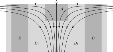
Figure 3. An illustration of Lemma 3.7 in the case where $L$ lies inside the fiber infinity, the latter depicted by the horizontal line at the top. The lighter shaded region is the wavefront set of $B_{1}$, while the darker shaded regions are the wavefront sets of $A$ and $B$. Several trajectories of the flow are displayed; $\Omega$ is the vertical trajectory converging to $L$.

Remarks. (i) The condition $\mathbf{u}\in C^{\infty}(\mathcal{M})$ can be relaxed as follows: let $m<s$ and $\operatorname{Im}\mathbf{P}\lesssim-h$ on $H^{s^{\prime}}_{h}$ near $L$ for all $s^{\prime}\in[m,s]$, and the symbol of the corresponding operators $\mathbf{Z}$ is invertible on $L$ uniformly in $s^{\prime}$. Then the conditions $A\mathbf{u}\in H^{m}_{h}$, $B\mathbf{u}\in H^{s}_{h}$, $B_{1}\mathbf{P}u\in H^{s}_{h}$ imply that $A\mathbf{u}\in H^{s}_{h}$, and (3.12) holds. The proof works by improving the Sobolev regularity of $\mathbf{u}$ in small steps $\delta>0$ (depending on the operators in (3.7)) by an approximation argument similar to the one in the proofs of [Va, Propositions 2.3–2.4]. For our purposes, it suffices to show (3.12) for $\mathbf{u}\in C^{\infty}$, so we avoid this approximation argument.

(ii) Lemma 3.7 implies several other semiclassical estimates:

• propagation of singularities (Lemma 3.2), by taking $L=\emptyset$;

• radial points estimate (see [Me, Proposition 9] and [DyZw13, Proposition 2.6]), by taking $L$ to be a radial source, $B=0$, $\Omega=\{\langle\xi\rangle^{-1}p=0\}$, and using part 1 of Lemma 3.6;

• dual radial points estimate (see [Me, Proposition 10] and [DyZw13, Proposition 2.7]), by taking $L$ to be a radial sink, $B$ microlocalized inside a punctured neighborhood of $L$, $\Omega\cap\operatorname{WF}_{h}(A)=L\cap\{\langle\xi\rangle^{-1}p=0\}$, and using part 2 of Lemma 3.6.

The first implication is circular, since the proof uses propagation of singularities.

The proof of Lemma 3.7 relies on the construction of a special escape function:

Lemma 3.8.

Under the assumptions of Lemma 3.7, let $U\subset\overline{T}^{*}\mathcal{M}$ be an open neighborhood of $L$. Then there exists a function $\chi\in C^{\infty}(\overline{T}^{*}\mathcal{M};[0,1])$ such that:

1. $\operatorname{supp}\chi\subset U$;

2. $\chi=1$ near $L$;

3. $H_{p}\chi\leq 0$ in some neighborhood of $\Omega$.

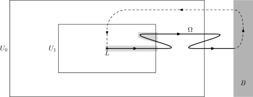
Figure 4. An illustration of the proof of Lemma 3.8. The darker shaded region is $\operatorname{WF}_{h}(B)$ and the lighter shaded region is $\operatorname{supp}\chi_{1}$. A possible trajectory of $H_{p}$ is shown; $\Omega$ is the undashed part of this trajectory.

Proof.

We take open neighborhoods (see Figure 4)

$$U_{1}\ \subset\ U_{0}\ \subset\ \operatorname{ell}_{h}(A)\setminus\operatorname{WF}_{h}(B)$$

of $L$ such that

$$e^{-tH_{p}}(\Omega\cap\overline{U_{0}})\ \subset\ U\quad\text{and}\quad e^{-tH_{p}}(\Omega\cap\overline{U_{1}})\ \subset\ U_{0}\quad\text{for all }t\geq 0.$$ (3.13)

The first equation in (3.13) follows from (3.11) for $t$ large enough independently of $U_{0}$; for bounded $t$, it suffices to use the fact that $L$ is invariant under the flow and take $U_{0}$ small enough. The set $U_{1}$ is constructed in the same way.

By (3.11), there exists $T>0$ such that

$$e^{-TH_{p}}(\Omega\cap\overline{U_{0}})\ \subset\ U_{1}.$$ (3.14)

Take a function $\chi_{1}\in C_{0}^{\infty}(U_{0};[0,1])$ such that $\chi_{1}=1$ near $(\Omega\cap\overline{U_{1}})\cup L$ and

$$e^{-tH_{p}}(\operatorname{supp}\chi_{1})\ \subset\ U_{0}\quad\text{for all }t\in[0,T].$$ (3.15)

The existence of such function follows from the second equation in (3.13) and the invariance of $L$ under the flow.

We have

$$e^{tH_{p}}(\Omega)\cap\operatorname{supp}\chi_{1}\ \subset\ \Omega\quad\text{for all }t\in[0,T].$$ (3.16)

Indeed, assume that $(x,\xi)\in\operatorname{supp}\chi_{1}$ and $e^{-tH_{p}}(x,\xi)\in\Omega$, but $(x,\xi)\notin\Omega$. Since the set $\{\langle\xi\rangle^{-1}p=0\}$ is invariant under the flow and contains $e^{-tH_{p}}(x,\xi)$, we have $(x,\xi)\in\operatorname{Con}_{p}(\operatorname{ell}_{h}(B);\operatorname{ell}_{h}(B_{1}))$. By Definition 3.1, there exists $T^{\prime}\geq 0$ such that $e^{-T^{\prime}H_{p}}(x,\xi)\in\operatorname{ell}_{h}(B)$ and $e^{-t^{\prime}H_{p}}(x,\xi)\in\operatorname{ell}_{h}(B_{1})$ for all $t^{\prime}\in[0,T^{\prime}]$. By (3.15), we have $e^{-sH_{p}}(x,\xi)\notin\operatorname{ell}_{h}(B)$ for $s\in[0,T]$, which implies that $T^{\prime}>T\geq t$. Then $e^{-tH_{p}}(x,\xi)\in\operatorname{Con}_{p}(\operatorname{ell}_{h}(B);\operatorname{ell}_{h}(B_{1}))$, which contradicts the fact that $e^{-tH_{p}}(x,\xi)\in\Omega$.

Combining (3.14) and (3.16), we get

$$\Omega\cap e^{-TH_{p}}(\operatorname{supp}\chi_{1})\ \subset\ \Omega\cap e^{-TH_{p}}(\Omega\cap\operatorname{supp}\chi_{1})\ \subset\ \Omega\cap U_{1}.$$ (3.17)

Combining (3.16) with the first part of (3.13), we get

$$\Omega\cap e^{-tH_{p}}(\operatorname{supp}\chi_{1})\ \subset\ e^{-tH_{p}}(\Omega\cap\operatorname{supp}\chi_{1})\ \subset U\quad\text{for all }t\in[0,T].$$ (3.18)

It follows from (3.17) that for $(x,\xi)$ near $\Omega\cap\operatorname{supp}(\chi_{1}\circ e^{TH_{p}})$, we have $\chi_{1}(x,\xi)=1$. Since $0\leq\chi_{1}\leq 1$, we have for $(x,\xi)$ in some neighborhood of $\Omega$,

$$\chi_{1}(x,\xi)\geq\chi_{1}(e^{TH_{p}}(x,\xi)).$$ (3.19)

Put

$$\widetilde{\chi}={1\over T}\int_{0}^{T}\chi_{1}\circ e^{tH_{p}}\,dt,\quad H_{p}\widetilde{\chi}={\chi_{1}\circ e^{TH_{p}}-\chi_{1}\over T},$$

then $H_{p}\widetilde{\chi}\leq 0$ in some neighborhood of $\Omega$. By (3.18), $\Omega\cap\operatorname{supp}\widetilde{\chi}\subset U$. Since $\chi_{1}=1$ near $L$, we also have $\widetilde{\chi}=1$ near $L$. It remains to put $\chi:=\chi_{2}\widetilde{\chi}$, where $\chi_{2}\in C_{0}^{\infty}(U;[0,1])$ satisfies $\chi_{2}=1$ near $(\Omega\cap\operatorname{supp}\widetilde{\chi})\cup L$. ∎

We now give

Proof of Lemma 3.7.

We start with the estimate

$$\|\mathbf{A}_{1}\mathbf{u}\|_{H^{s}_{h}}\leq C\|B\mathbf{u}\|_{H^{s}_{h}}+Ch^{-1}\|B_{1}\mathbf{P}\mathbf{u}\|_{H^{s}_{h}}+\mathcal{O}(h^{\infty})\|\mathbf{u}\|_{H^{-N}_{h}}$$ (3.20)

valid for all $\mathbf{A}_{1}\in\Psi^{0}_{h}(\mathcal{M};\mathcal{E})$ such that $\operatorname{WF}_{h}(\mathbf{A}_{1})\subset\operatorname{ell}_{h}(B_{1})\setminus\Omega$. Indeed, we have

$$\operatorname{WF}_{h}(\mathbf{A}_{1})\ \subset\ (\operatorname{ell}_{h}(B_{1})\cap\operatorname{ell}_{h}(\mathbf{P}))\cup\operatorname{Con}_{p}(\operatorname{ell}_{h}(B);\operatorname{ell}_{h}(B_{1})),$$

therefore by a partition of unity we may reduce to the situation when $\operatorname{WF}_{h}(\mathbf{A}_{1})$ is contained either inside $\operatorname{ell}_{h}(B_{1})\setminus\{\langle\xi\rangle^{-1}p=0\}$ or inside $\operatorname{Con}_{p}(\operatorname{ell}_{h}(B);\operatorname{ell}_{h}(B_{1}))$. The first case is handled by the elliptic estimate [DyZw13, Proposition 2.4] and the second one, by propagation of singularities (Lemma 3.2).

Similarly we have the estimate

$$\|A\mathbf{u}\|_{H^{s}_{h}}\leq C\|B\mathbf{u}\|_{H^{s}_{h}}+C\|\mathbf{A}_{2}\mathbf{u}\|_{H^{s}_{h}}+Ch^{-1}\|B_{1}\mathbf{P}\mathbf{u}\|_{H^{s}_{h}}+\mathcal{O}(h^{\infty})\|\mathbf{u}\|_{H^{-N}_{h}}$$ (3.21)

valid for all $\mathbf{A}_{2}\in\Psi^{0}_{h}(\mathcal{M};\mathcal{E})$ such that $L\subset\operatorname{ell}_{h}(\mathbf{A}_{2})$, where we use the following corollary of (3.11):

$$\operatorname{WF}_{h}(A)\ \subset\ (\operatorname{ell}_{h}(B_{1})\cap\operatorname{ell}_{h}(\mathbf{P}))\cup\operatorname{Con}_{p}(\operatorname{ell}_{h}(B);\operatorname{ell}_{h}(B_{1}))\cup\operatorname{Con}_{p}(\operatorname{ell}_{h}(\mathbf{A}_{2});\operatorname{ell}_{h}(B_{1})).$$

Next, using Definition 3.3, choose $\mathbf{Y}_{1}\in\Psi^{s}_{h}(\mathcal{M};\mathcal{E})$, $\mathbf{Y}_{2}\in\Psi^{-s}_{h}(\mathcal{M};\mathcal{E})$, and $\mathbf{Z}\in\Psi^{0}_{h}(\mathcal{M};\mathcal{E})$ such that

$$\mathbf{Y}_{1}\mathbf{Y}_{2}=1+\mathcal{O}(h^{\infty})\quad\text{near }\overline{U},\quad\overline{U}\subset\operatorname{ell}_{h}(\mathbf{Z}),$$

for some neighborhood $U\subset\operatorname{ell}_{h}(A)\cap\operatorname{ell}_{h}(B_{1})$ of $L$, and for each $\mathbf{v}\in C^{\infty}(\mathcal{M};\mathcal{E})$,

$$\operatorname{Im}\langle\mathbf{P}^{\prime}\mathbf{v},\mathbf{v}\rangle_{L^{2}}\leq-h\|\mathbf{Z}\mathbf{v}\|_{L^{2}}^{2}+\mathcal{O}(h^{\infty})\|\mathbf{v}\|^{2}_{H^{-N}_{h}},$$ (3.22)

where $\mathbf{P}^{\prime}:=\mathbf{Y}_{1}\mathbf{P}\mathbf{Y}_{2}\in\Psi^{1}_{h}(\mathcal{M};\mathcal{E})$. Note that $\sigma_{h}(\mathbf{P}^{\prime})=\sigma_{h}(\mathbf{P})$ on $U$.

We now claim that it suffices to show that there exist operators

$$A_{1},A_{2},B_{2}\in\Psi^{0}_{h}(\mathcal{M}),\quad\operatorname{WF}_{h}(A_{1})\subset U\setminus\Omega,\quad L\subset\operatorname{ell}_{h}(A_{2}),\quad\operatorname{WF}_{h}(B_{2})\subset U,$$

such that for each $\mathbf{v}\in C^{\infty}(\mathcal{M};\mathcal{E})$,

$$\|A_{2}\mathbf{v}\|_{L^{2}}\leq C\|A_{1}\mathbf{v}\|_{L^{2}}+Ch^{-1}\|B_{2}\mathbf{P}^{\prime}\mathbf{v}\|_{L^{2}}+Ch^{1/2}\|B_{2}\mathbf{v}\|_{H^{-1/2}_{h}}+\mathcal{O}(h^{\infty})\|\mathbf{v}\|_{H^{-N}_{h}}.$$ (3.23)

Indeed, applying (3.23) to $\mathbf{v}:=\mathbf{Y}_{1}\mathbf{u}$ and assuming that $\operatorname{WF}_{h}(A_{2})\subset U$, we get

$$\|\mathbf{A}_{2}\mathbf{u}\|_{H^{s}_{h}}\leq C\|\mathbf{A}_{1}\mathbf{u}\|_{H^{s}_{h}}+Ch^{-1}\|B_{1}\mathbf{P}\mathbf{u}\|_{H^{s}_{h}}+Ch^{1/2}\|A\mathbf{u}\|_{H^{s-1/2}_{h}}+\mathcal{O}(h^{\infty})\|\mathbf{u}\|_{H^{-N}_{h}}.$$ (3.24)

where $\mathbf{A}_{j}:=\mathbf{Y}_{2}A_{j}\mathbf{Y}_{1}$ satisfy $\operatorname{WF}_{h}(\mathbf{A}_{1})\subset U\setminus\Omega$, $L\subset\operatorname{ell}_{h}(\mathbf{A}_{2})$. Here we used the fact that $\operatorname{WF}_{h}(B_{2})\subset\operatorname{ell}_{h}(A)$ and the elliptic estimate to bound $\|B_{2}\mathbf{v}\|_{H^{-1/2}_{h}}$ in terms of $\|A\mathbf{u}\|_{H^{s-1/2}_{h}}$. To obtain the required estimate (3.12), it remains to combine this with (3.20) and (3.21), and take $h$ small enough to eliminate the $Ch^{1/2}\|A\mathbf{u}\|_{H^{s-1/2}_{h}}$ remainder.

We now prove (3.23) using a positive commutator argument. Let $\chi$ be the function constructed in Lemma 3.8. Fix $F\in\Psi^{0}_{h}(\mathcal{M})$ such that

$$\sigma_{h}(F)=\chi,\quad\operatorname{WF}_{h}(F)\subset U.$$

Then

$$\sigma_{h}(ih^{-1}[\operatorname{Re}\mathbf{P}^{\prime},F^{*}F])=2\chi H_{p}\chi\leq 0\quad\text{near }\Omega.$$

Therefore

$$[\operatorname{Re}\mathbf{P}^{\prime},F^{*}F]=-ih(\mathbf{G}_{1}+\mathbf{G}_{2}),$$ (3.25)

where $\mathbf{G}_{j}\in\Psi^{0}_{h}(\mathcal{M};\mathcal{E})$ are self-adjoint and principally scalar, and

$$\operatorname{WF}_{h}(\mathbf{G}_{j})\subset U;\quad\sigma_{h}(\mathbf{G}_{1})\leq 0;\quad\operatorname{WF}_{h}(\mathbf{G}_{2})\cap\Omega=\emptyset.$$

For each $\mathbf{v}\in C^{\infty}(\mathcal{M};\mathcal{E})$, we have

$$\operatorname{Im}\langle\mathbf{P}^{\prime}\mathbf{v},F^{*}F\mathbf{v}\rangle_{L^{2}}={i\over 2}\langle[\operatorname{Re}\mathbf{P}^{\prime},F^{*}F]\mathbf{v},\mathbf{v}\rangle_{L^{2}}+\operatorname{Re}\langle F^{*}F(\operatorname{Im}\mathbf{P}^{\prime})\mathbf{v},\mathbf{v}\rangle_{L^{2}}.$$ (3.26)

Take $A_{1},B_{2}\in\Psi^{0}_{h}(\mathcal{M})$ such that

$$\begin{gathered}\operatorname{WF}_{h}(A_{1})\ \subset\ U\setminus\Omega,\quad A_{1}=1+\mathcal{O}(h^{\infty})\quad\text{near }\operatorname{WF}_{h}(\mathbf{G}_{2});\\ \operatorname{WF}_{h}(B_{2})\ \subset\ U,\quad B_{2}=1+\mathcal{O}(h^{\infty})\quad\text{near }\operatorname{WF}_{h}(F)\cup\operatorname{WF}_{h}(\mathbf{G}_{1})\cup\operatorname{WF}_{h}(\mathbf{G}_{2}).\end{gathered}$$

By the sharp Gårding inequality (Lemma 3.4) applied to $\mathbf{G}_{1}$ and the elliptic estimate applied to $\mathbf{G}_{2}$, the product ${i\over 2}\langle[\operatorname{Re}\mathbf{P}^{\prime},F^{*}F]\mathbf{v},\mathbf{v}\rangle_{L^{2}}$ is equal to

$${h\over 2}\big{(}\langle\mathbf{G}_{1}B_{2}\mathbf{v},B_{2}\mathbf{v}\rangle_{L^{2}}+\langle\mathbf{G}_{2}A_{1}\mathbf{v},A_{1}\mathbf{v}\rangle_{L^{2}}\big{)}+\mathcal{O}(h^{\infty})\|\mathbf{v}\|_{H^{-N}_{h}}^{2}$$ (3.27)

$$\leq Ch^{2}\|B_{2}\mathbf{v}\|_{H^{-1/2}_{h}}^{2}+Ch\|A_{1}\mathbf{v}\|_{L^{2}}^{2}+\mathcal{O}(h^{\infty})\|\mathbf{v}\|_{H^{-N}_{h}}^{2}.$$

Next, $h^{-1}F^{*}[F,\operatorname{Im}\mathbf{P}^{\prime}]\in\Psi^{0}_{h}$ and its principal symbol is imaginary valued, therefore $\operatorname{Re}(F^{*}[F,\operatorname{Im}\mathbf{P}^{\prime}])\in h^{2}\Psi^{-1}_{h}$. It then follows from (3.22) that

$$\begin{gathered}\operatorname{Re}\langle F^{*}F(\operatorname{Im}\mathbf{P}^{\prime})\mathbf{v},\mathbf{v}\rangle_{L^{2}}=\operatorname{Im}\langle\mathbf{P}^{\prime}F\mathbf{v},F\mathbf{v}\rangle_{L^{2}}+\langle\operatorname{Re}(F^{*}[F,\operatorname{Im}\mathbf{P}^{\prime}])\mathbf{v},\mathbf{v}\rangle_{L^{2}}\\ \leq-h\|\mathbf{Z}F\mathbf{v}\|_{L^{2}}^{2}+Ch^{2}\|B_{2}\mathbf{v}\|_{H^{-1/2}_{h}}^{2}+\mathcal{O}(h^{\infty})\|\mathbf{v}\|_{H^{-N}_{h}}^{2}.\end{gathered}$$ (3.28)

Since $\mathbf{Z}$ is elliptic on $U\supset\operatorname{WF}_{h}(F)$, we have

$$\|F\mathbf{v}\|_{L^{2}}^{2}\leq C\|\mathbf{Z}F\mathbf{v}\|_{L^{2}}^{2}+\mathcal{O}(h^{\infty})\|\mathbf{v}\|_{H^{-N}_{h}}^{2}.$$

Combining this with (3.26)–(3.28), we get

$$\begin{gathered}C^{-1}h\|F\mathbf{v}\|_{L^{2}}^{2}-Ch\|A_{1}\mathbf{v}\|_{L^{2}}^{2}-Ch^{2}\|B_{2}\mathbf{v}\|_{H^{-1/2}_{h}}^{2}\\ \leq-\operatorname{Im}\langle\mathbf{P}^{\prime}\mathbf{v},F^{*}F\mathbf{v}\rangle+\mathcal{O}(h^{\infty})\|\mathbf{v}\|_{H^{-N}_{h}}^{2}\\ \leq C\|B_{2}\mathbf{P}^{\prime}\mathbf{v}\|_{L^{2}}\cdot\|F\mathbf{v}\|_{L^{2}}+\mathcal{O}(h^{\infty})\|\mathbf{v}\|_{H^{-N}_{h}}^{2},\end{gathered}$$

which implies (3.23) with $A_{2}:=F$, finishing the proof. ∎

4. Properties of the resolvent

In this section, we prove Theorems 1 and 2, and show microlocalization statements for the resolvent that form the basis of the proof of Theorem 3 in the next section. We follow in part the argument of [DyZw13], based on the strategy of [FaSj].

4.1. Auxiliary resolvent

In this section, we introduce an auxiliary resolvent depending on the semiclassical parameter $h>0$. Recall the function $\rho$, the constant $\varepsilon$, and the vector field $X_{1}$ used in Lemma 2.1, and let $p$ be defined in (2.8).

Anisotropic spaces. We first construct the anisotropic Sobolev spaces on which the auxiliary resolvent will be defined. The order function of these spaces is given by the following (see Figure 5(a))

Lemma 4.1.

There exists $m\in C^{\infty}(S^{*}\mathcal{M};\mathbb{R})$ such that, with $H_{p}$ pulled back to $S^{*}\mathcal{M}$ by the projection $\kappa:T^{*}\mathcal{M}\setminus 0\to S^{*}\mathcal{M}$, and $E_{\pm}^{*}$ defined in Lemma 2.10,

1. $m=1$ in a neighborhood of $\kappa(E_{-}^{*})\supset\kappa(E_{s}^{*})$;

2. $m=-1$ in a neighborhood of $\kappa(E_{+}^{*})\supset\kappa(E_{u}^{*})$;

3. $H_{p}m\leq 0$ in a neighborhood of $\{p=0\}$;

4. $\operatorname{supp}m\subset\{\rho>-2\varepsilon\}$ and $\operatorname{supp}m\cap\{\rho=-\varepsilon\}\cap\{X_{1}\rho=0\}=\emptyset$.

Proof.

Let $m_{\pm}$ be the functions constructed in Lemma 2.12, then

1. $m_{-}=1$ and $m_{+}=0$ in a neighborhood of $\kappa(E_{-}^{*})$;

2. $m_{+}=1$ and $m_{-}=0$ in a neighborhood of $\kappa(E_{+}^{*})$;

3. $\pm H_{p}m_{\pm}\geq 0$ on $V\setminus\pi^{-1}(V_{\pm})$, where $V$ is a neighborhood of $\{p=0\}$ and $V_{\pm}:=\pi(\operatorname{supp}m_{\pm})\setminus\mathcal{U}\subset\Sigma_{\pm}\setminus\mathcal{U}$ are compact. Here $\pi:S^{*}\mathcal{M}\to\mathcal{M}$ is the projection map and $\Sigma_{\pm}$ are defined in (2.4).

Next, take the functions $\chi_{\pm}$ constructed in Lemma 2.8 (with the sets $V_{\pm}$ defined in (3) above). We have $\pm H_{p}(\chi_{\pm}\circ\pi)\geq 0$ everywhere, $\chi_{\pm}=0$ near $K$, and $\pm H_{p}(\chi_{\pm}\circ\pi)>\delta>0$ on $\pi^{-1}(V_{\pm})$. Then for a large enough constant $R>0$, the function

$$m:=m_{-}-m_{+}+R(\chi_{-}\circ\pi-\chi_{+}\circ\pi)$$

satisfies conditions (1)–(3). Condition (4) follows immediately from the fact that $\operatorname{supp}m_{\pm}\subset\pi^{-1}(\Sigma_{\pm})\subset\{\rho>-\varepsilon\}$ and $\operatorname{supp}\chi_{\pm}\subset\{\rho>-2\varepsilon\}\cap\{\pm X_{1}\rho<0\}$. ∎

We now consider $m$ as a homogeneous function of degree 0 on $T^{*}\mathcal{M}$ and define the weight $\widetilde{m}\in C^{\infty}(T^{*}\mathcal{M})$ by

$$\widetilde{m}(x,\xi)=(1-\chi_{m}(x,\xi))m(x,\xi)\log|\xi|,$$ (4.1)

where $\chi_{m}\in C_{0}^{\infty}(T^{*}\mathcal{M};[0,1])$ is equal to 1 near the zero section and supported in $\{|\xi|<1\}$.

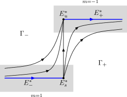
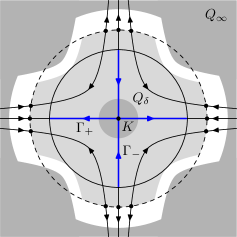
(a)(b)

Figure 5. (a) The flow $e^{tH_{p}}$ on $S^{*}\mathcal{M}\cap\{p=0\}$. The left half of the figure represents the sphere bundle over $\Gamma_{-}$, the right half represents $\Gamma_{+}$, and the vertical midline represents $K$. (To obtain this from Figure 2, glue the rear halves of the two vertical planes.) The thick blue lines are $E_{\pm}^{*}$ and the shaded boxes represent the regions where $m=\pm 1$. (b) The flow $\varphi^{t}$ near $\mathcal{U}$ (pictured by the solid circle). The dashed circle is $\{\rho=-\varepsilon\}$, consisting of fixed points; $q_{1}$ is supported near this circle. The lighter shaded region denotes the set $\Sigma$ from (2.4), while the darker shaded regions denote the supports of $Q_{\infty}$ and $Q_{\delta}$ (the latter microlocalized near zero frequency).

Take an operator

$$G=G(h)\in\bigcap_{\delta>0}\Psi^{\delta}_{h}(\mathcal{M}),\quad\sigma_{h}(G)=\widetilde{m},\quad\operatorname{WF}_{h}(G)\cap\{\xi=0\}=\emptyset.$$ (4.2)

We moreover require that

$$\operatorname{WF}_{h}(G)\ \subset\ \{\rho>-2\varepsilon\},\quad\operatorname{WF}_{h}(G)\cap\{\rho=-\varepsilon\}\cap\{X_{1}\rho=0\}=\emptyset.$$ (4.3)

For each $r\in\mathbb{R}$, we define the anisotropic Sobolev space $\mathcal{H}^{r}_{h}$ as follows:

$$\mathcal{H}^{r}_{h}:=\exp(-rG(h))(L^{2}(\mathcal{M};\mathcal{E})),\quad\|\mathbf{u}\|_{\mathcal{H}^{r}_{h}}:=\|\exp(rG(h))\mathbf{u}\|_{L^{2}(\mathcal{M};\mathcal{E})}.$$ (4.4)

As explained for instance in [DyZw13, Sections 3.1 and 3.3], we have

$$H^{C_{m}|r|}_{h}(\mathcal{M};\mathcal{E})\subset\mathcal{H}^{r}_{h}\subset H^{-C_{m}|r|}_{h}(\mathcal{M};\mathcal{E})$$ (4.5)

where $H^{r}_{h}$ stands for the standard semiclassical Sobolev space [Zw, Section 14.2.4] and $C_{m}=\sup_{S^{*}\mathcal{M}}|m|$; we can take $C_{m}=1$ for distributions supported inside $\mathcal{U}$. Moreover, the norms of $\mathcal{H}^{r}_{h}$ for different $h$ are all equivalent with constants depending on $h$.

Since $m=1$ near $\kappa(E_{-}^{*})$, we have $\widetilde{m}=\log|\xi|$ near $\kappa(E_{-}^{*})\subset\partial\overline{T}^{*}\mathcal{M}$, where

$$\kappa:T^{*}\mathcal{M}\setminus 0\ \to\ S^{*}\mathcal{M}=\partial\overline{T}^{*}\mathcal{M}$$ (4.6)

is the projection map. It follows from [Zw, Theorems 8.6 and 8.10] that $\mathcal{H}^{r}_{h}$ is microlocally equivalent to the standard semiclassical Sobolev space $H^{r}_{h}$ near $\kappa(E_{-}^{*})$ in the following sense: for each $A\in\Psi^{0}_{h}(\mathcal{M})$ such that $\operatorname{WF}_{h}(A)$ is contained in a small neighborhood of $\kappa(E_{-}^{*})$ and all $\mathbf{u}\in C^{\infty}(\mathcal{M};\mathcal{E})$, we have

$$\|A\mathbf{u}\|_{\mathcal{H}^{r}_{h}}\leq C\|\mathbf{u}\|_{H^{r}_{h}},\quad\|A\mathbf{u}\|_{H^{r}_{h}}\leq C\|\mathbf{u}\|_{\mathcal{H}^{r}_{h}}.$$ (4.7)

Since $m=-1$ near $\kappa(E_{+}^{*})$, we similarly have for each $A\in\Psi^{0}_{h}(\mathcal{M})$ with $\operatorname{WF}_{h}(A)$ contained in a small neighborhood of $\kappa(E_{+}^{*})$,

$$\|A\mathbf{u}\|_{\mathcal{H}^{r}_{h}}\leq C\|\mathbf{u}\|_{H^{-r}_{h}},\quad\|A\mathbf{u}\|_{H^{-r}_{h}}\leq C\|\mathbf{u}\|_{\mathcal{H}^{r}_{h}}.$$ (4.8)

Complex absorbing operators. Take small $\delta>0$ and choose

$$Q_{\infty}\in\Psi^{1}_{h}(\mathcal{M}),\quad Q_{\delta}\in\Psi^{\operatorname{comp}}_{h}(\mathcal{M}),\quad q_{1}\in C^{\infty}(\mathcal{M})$$ (4.9)

such that $\sigma_{h}(Q_{\infty}),\sigma_{h}(Q_{\delta}),q_{1}\geq 0$ everywhere and

1. $\operatorname{1\hskip-2.75ptl}_{\Sigma^{\prime}}Q_{\infty}=Q_{\infty}\operatorname{1\hskip-2.75ptl}_{\Sigma^{\prime}}=0$, where $\Sigma^{\prime}$ is a neighborhood of $\overline{\Sigma}$ and $\Sigma$ is defined in (2.4);

2. $\{\rho\leq-2\varepsilon\}\cup\big{(}\{\rho=-\varepsilon\}\cap\{X_{1}\rho=0\}\big{)}\ \subset\ \operatorname{ell}_{h}(Q_{\infty})$;

3. $Q_{\delta}=\chi_{\delta}Q_{\delta}\chi_{\delta}$ for some $\chi_{\delta}\in C^{\infty}(\mathcal{M})$ supported in a $\delta$-neighborhood of $K$, $\operatorname{WF}_{h}(Q_{\delta})\ \subset\ \{|\xi|<\delta\}$, and $\{x\in K,\ \xi=0\}\ \subset\ \operatorname{ell}_{h}(Q_{\delta})$;

4. $\operatorname{supp}q_{1}\cap\overline{\mathcal{U}}=\emptyset$ and $q_{1}>0$ on $\{\rho=-\varepsilon\}$;

5. $\operatorname{WF}_{h}(G)\cap(\operatorname{WF}_{h}(Q_{\delta})\cup\operatorname{WF}_{h}(Q_{\infty}))=\emptyset$.

The existence of $Q_{\infty}$ is guaranteed by Lemma 2.7 and the fact that $\Sigma\subset\{\rho>-\varepsilon\}$. Condition (5) can be satisfied by (4.2) and (4.3). See Figure 5(b).

The use of the absorbing operator $Q_{\delta}$ goes back to [FaSj]; we will follow closely the later argument of [DyZw13]. By contrast, the operator $Q_{\infty}$ is something specific to open systems; such complex absorbing operators have been previously used in scattering theory, see for instance [St, NoZw09, Va]. The absorbing potential $q_{1}$ guarantees invertibility on $\{\rho=-\varepsilon\}$; making $Q_{\infty}$ elliptic there would destroy the propagation of support property, meaning that Lemma 4.4 below would no longer be true.

Existence of the auxiliary resolvent. Introduce the modified operator

$$\mathbf{P}_{\delta}=\mathbf{P}_{\delta}(h)={h\over i}\mathbf{X}-i(Q_{\infty}+q_{1}+Q_{\delta})\in\Psi^{1}_{h}(\mathcal{M};\mathcal{E})$$ (4.10)

which acts $\mathcal{D}^{r}_{h}\to\mathcal{H}^{r}_{h}$, where

$$\mathcal{D}^{r}_{h}:=\{\mathbf{u}\in\mathcal{H}^{r}_{h}\mid\mathbf{P}_{\delta}\mathbf{u}\in\mathcal{H}^{r}_{h}\},\quad\|\mathbf{u}\|_{\mathcal{D}^{r}_{h}}:=\|\mathbf{u}\|_{\mathcal{H}^{r}_{h}}+\|\mathbf{P}_{\delta}\mathbf{u}\|_{\mathcal{H}^{r}_{h}}.$$ (4.11)

Note that, with $p$ defined in (2.8),

$$\sigma_{h}(\mathbf{P}_{\delta})=p-i(\sigma_{h}(Q_{\infty})+\sigma_{h}(Q_{\delta})+q_{1}).$$

The main result of this subsection is the following

Lemma 4.2.

Take $C_{1},C_{2}>0$. Then there exists $r_{0}=r_{0}(C_{1})\geq 0$ such that for all $r\geq r_{0}$ and $0<h<h_{0}(C_{1},C_{2},r)$, the inverse

$$\mathbf{R}_{\delta}(z)=(\mathbf{P}_{\delta}-z)^{-1}:\mathcal{H}^{r}_{h}\to\mathcal{D}^{r}_{h},\quad z\in[-C_{2}h,C_{2}h]+i[-C_{1}h,1]$$ (4.12)

exists and satisfies the bound

$$\|\mathbf{R}_{\delta}(z)\|_{\mathcal{H}^{r}_{h}\to\mathcal{H}^{r}_{h}}\leq Ch^{-1}.$$ (4.13)

Furthermore, the $h$-wavefront set of $\mathbf{R}_{\delta}(z)$ satisfies

$$\operatorname{WF}_{h}^{\prime}(\mathbf{R}_{\delta}(z))\cap T^{*}(\mathcal{U}\times\mathcal{U})\ \subset\ \Delta(T^{*}\mathcal{U})\cup\Upsilon_{+},$$ (4.14)

where $\Delta(T^{*}\mathcal{U})$ is the diagonal of $T^{*}\mathcal{U}$ and $\Upsilon_{+}$ is the positive flow-out of $e^{tH_{p}}$ on $\{p=0\}$ inside $\pi^{-1}(\mathcal{U})$ (here $\pi:\overline{T}^{*}\mathcal{M}\to\mathcal{M}$ is the projection map)

$$\Upsilon_{+}=\{(e^{tH_{p}}(y,\eta),y,\eta)\mid t\geq 0,\ p(y,\eta)=0,\ y\in\mathcal{U},\ \varphi^{t}(y)\in\mathcal{U}\}.$$

Remarks. (i) The proof of Lemma 4.2 can be summarized as follows:

• the anisotropic spaces give invertibility at the projections of the sets $E_{u}^{*},E_{s}^{*}$ to fiber infinity $\partial\overline{T}^{*}\mathcal{M}$;

• together, $q_{1}$ and $Q_{\infty}$ give invertibility on $\{\rho\leq-\varepsilon\}$;

• the operator $Q_{\delta}$ gives invertibility on the set $\{(x,0)\mid x\in K\}$; and

• invertibility elsewhere is obtained by propagation of singularities.

(ii) One can specify the value of $r_{0}$ more precisely. Indeed, the condition $r\geq r_{0}$ is only needed to ensure that (4.20), (4.21) hold. Examining the proof of Lemma 3.6, we see immediately that we can take for some large fixed constant $\widetilde{C}>0$,

$$r_{0}=\widetilde{C}(1+C_{1}).$$ (4.15)

Moreover, if $h^{-1}\operatorname{Im}z$ is large enough and positive, then we can take $r_{0}=0$.

(iii) If additionally $\mathbf{X}^{*}=-\mathbf{X}$ near $K$ with respect to some smooth measure on $\mathcal{U}$ and some inner product on the fibers of $\mathcal{E}$ (e.g. when $\mathcal{E}=\mathbb{R}$, $\mathbf{X}=X$, and $X$ admits a smooth invariant measure), then we can take for some $\widetilde{C}>0$, any $r_{0}$ with

$$r_{0}>\widetilde{C}C_{1}.$$ (4.16)

Furthermore, replacing $\gamma/2$ in the proof of Lemma 3.6 by a constant arbitrarily close to $\gamma$, we can put $\widetilde{C}:=\gamma^{-1}$, where $\gamma$ is the minimal expansion rate appearing in (1.5).

Proof.

We use the strategy of the proof of [DyZw13, Proposition 3.4]. One could similarly adapt the construction of [FaSj, Section 3], however the method of [DyZw13] is more convenient for the wavefront set statements, needed for Theorem 3.

To reduce $\mathcal{H}^{r}_{h}$ estimates to $L^{2}$ estimates, we use the conjugated operator (see [DyZw13, Section 3.3] for details)

$$\mathbf{P}_{\delta,r}=e^{rG}\mathbf{P}_{\delta}e^{-rG}=\mathbf{P}_{\delta}+r[G,\mathbf{P}_{\delta}]+\mathcal{O}(h^{2})_{\Psi^{-1+}_{h}}.$$ (4.17)

Since $\operatorname{WF}_{h}(G)\cap(\operatorname{WF}_{h}(Q_{\delta})\cup\operatorname{WF}_{h}(Q_{\infty}))=\emptyset$, $\sigma_{h}(Q_{\infty}),\sigma_{h}(Q_{\delta}),q_{1}$ are real-valued, and $q_{1}$ is a pseudodifferential operator of order 0, we get

$$\operatorname{Re}\sigma_{h}(\mathbf{P}_{\delta,r})=p+\mathcal{O}(h)_{S^{0}}.$$ (4.18)

Since $H_{p}m\leq 0$ near $\{p=0\}$, it follows from (4.1) that $H_{p}\widetilde{m}\leq 0$ modulo $S^{0}$ near $\{\langle\xi\rangle^{-1}p=0\}$. Together with the fact that $\sigma_{h}(Q_{\infty}),\sigma_{h}(Q_{\delta}),q_{1}\geq 0$, this implies

$$\operatorname{Im}\sigma_{h}(\mathbf{P}_{\delta,r})\leq 0\quad\text{near }\{\langle\xi\rangle^{-1}p=0\}.$$ (4.19)

Now, by (2.11), $L=\kappa(E_{s}^{*})$ satisfies (3.9), where $\kappa$ is defined in (4.6). By part 1 of Lemma 3.6, there exists $r_{0}:=r_{0}(C_{1})$ such that

$$\operatorname{Im}(\mathbf{P}_{\delta}-z)\lesssim-h\quad\text{near }\kappa(E_{s}^{*})\quad\text{on }H^{r}_{h},\quad r\geq r_{0},\quad\operatorname{Im}z\geq-C_{1}h;$$ (4.20)

here we use Definition 3.3. Similarly, $L=\kappa(E_{u}^{*})$ satisfies (3.10). By part 2 of Lemma 3.6,

$$\operatorname{Im}(\mathbf{P}_{\delta}-z)\lesssim-h\quad\text{near }\kappa(E_{u}^{*})\quad\text{on }H^{-r}_{h},\quad r\geq r_{0},\quad\operatorname{Im}z\geq-C_{1}h.$$ (4.21)

Since (4.19) is true when $q_{1}$ is removed from $\mathbf{P}_{\delta}$, and $\operatorname{Re}\sigma_{h}(e^{rG}q_{1}e^{-rG})=q_{1}(x)>0$ on $\{\rho=-\varepsilon\}\subset\{\langle\xi\rangle^{-1}p=0\}\subset\overline{T}^{*}\mathcal{M}$, we have by Lemma 3.5,

$$\operatorname{Im}(\mathbf{P}_{\delta,r}-z)\lesssim-h\quad\text{near }\{\rho=-\varepsilon\}\quad\text{on }L^{2},\quad\operatorname{Im}z\geq-C_{1}h.$$ (4.22)

Finally, since $\{\rho=-\varepsilon\}\cap\{X_{1}\rho=0\}\subset\operatorname{ell}_{h}(Q_{\infty})$, there exist compact sets (see Figure 6)

$$L_{\pm}\ \subset\ \{\rho=-\varepsilon\}\cap\{\pm X_{1}\rho<0\}\ \subset\ \mathcal{M}$$ (4.23)

such that on $\overline{T}^{*}\mathcal{M}$, and with $L_{\pm}^{\circ}$ denoting the interior of $L_{\pm}$ inside $\{\rho=-\varepsilon\}$,

$$\{\rho=-\varepsilon\}\cap\{\pm X_{1}\rho\leq 0\}\ \subset\ \pi^{-1}(L_{\pm}^{\circ})\cup\operatorname{ell}_{h}(Q_{\infty}).$$ (4.24)

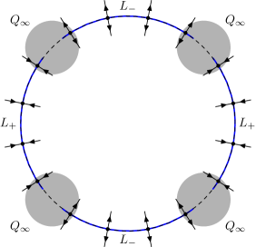
Figure 6. The sets $L_{\pm}$ (thick blue lines) and the elliptic set of $Q_{\infty}$ (shaded) near $\{\rho=-\varepsilon\}$ (dashed circle). The arrows depict the flow $\varphi^{t}$.

The proof of the lemma is based on the following bound similar to [DyZw13, (3.10)]:

$$\|\mathbf{u}\|_{\mathcal{H}^{r}_{h}}\leq Ch^{-1}\|\mathbf{f}\|_{\mathcal{H}^{r}_{h}},\quad\mathbf{u}\in\mathcal{D}^{r}_{h},\quad\mathbf{f}=(\mathbf{P}_{\delta}-z)\mathbf{u}.$$ (4.25)

By [FaSj, Lemma A.1] applied to $e^{rG}\mathbf{u}$ and the operator $\mathbf{P}_{\delta,r}\in\Psi^{1}_{h}$, for each fixed $h$ and each $\mathbf{u}\in\mathcal{D}^{r}_{h}$ there exists a sequence $\mathbf{u}_{j}\in C^{\infty}(\mathcal{M};\mathcal{E})$ such that $\mathbf{u}_{j}\to\mathbf{u}$ in $\mathcal{H}^{r}_{h}$ and $(\mathbf{P}_{\delta}-z)\mathbf{u}_{j}\to\mathbf{f}$ in $\mathcal{H}^{r}_{h}$. Therefore, it suffices to prove (4.25) for the case $\mathbf{u}\in C^{\infty}(\mathcal{M};\mathcal{E})$.

We now use semiclassical estimates to obtain bounds on $A\mathbf{u}$, where $A\in\Psi^{0}_{h}(\mathcal{M})$ falls into one of the following cases. We will typically arrive to a propagation estimate of the form

$$\|A\mathbf{u}\|_{\mathcal{H}^{r}_{h}}\leq C\|B\mathbf{u}\|_{\mathcal{H}^{r}_{h}}+Ch^{-1}\|B_{1}\mathbf{f}\|_{\mathcal{H}^{r}_{h}}+\mathcal{O}(h^{\infty})\|\mathbf{u}\|_{\mathcal{H}^{r}_{h}},$$ (4.26)

for some choice of operators $B,B_{1}\in\Psi^{0}_{h}(\mathcal{M})$. The term $B\mathbf{u}$ will be controlled by previously considered cases and we keep track of the wavefront set of $B_{1}$ to show (4.14).

Case 1: $\operatorname{WF}_{h}(A)\cap\{\langle\xi\rangle^{-1}p=0\}\ \subset\ \operatorname{ell}_{h}(Q_{\infty})\cup\operatorname{ell}_{h}(Q_{\delta})$. Then $\mathbf{P}_{\delta}-z$, and thus $\mathbf{P}_{\delta,r}-z$, is elliptic on $\operatorname{WF}_{h}(A)$. Similarly to [DyZw13, Proposition 3.4, Case 1], we find for some $B_{1}\in\Psi^{0}_{h}(\mathcal{M})$ microlocalized in a small neighborhood of $\operatorname{WF}_{h}(A)$,

$$\|A\mathbf{u}\|_{\mathcal{H}^{r}_{h}}\leq C\|B_{1}\mathbf{f}\|_{\mathcal{H}^{r}_{h}}+\mathcal{O}(h^{\infty})\|\mathbf{u}\|_{\mathcal{H}^{r}_{h}}.$$ (4.27)

Note that the $\mathcal{H}^{r}_{h}$ bound on the operator $\mathbf{P}_{\delta}-z$ is equivalent to the $L^{2}$ bound on the operator $\mathbf{P}_{\delta,r}-z$; we will use this fact in the next cases.

Case 2: $\operatorname{WF}_{h}(A)$ is contained in a small neighborhood of $\pi^{-1}(L_{-})\subset\overline{T}^{*}\mathcal{M}$, where $L_{-}$ is defined in (4.23) and $\pi:\overline{T}^{*}\mathcal{M}\to\mathcal{M}$ is the projection map; moreover, $\pi^{-1}(L_{-})\subset\operatorname{ell}_{h}(A)$.

For each $(x,\xi)\in\operatorname{WF}_{h}(A)$, $\varphi^{t}(x)$ uniformly converges to $\{\rho=-\varepsilon\}\cap\{X_{1}\rho>0\}$ as $t\to-\infty$. Here we used that $L_{-}\subset\{X_{1}\rho>0\}$, $\varphi^{t}(x)=e^{tX}$, $X=\psi(\rho)X_{1}$, and $\operatorname{sgn}\psi(\rho)=\operatorname{sgn}(\rho+\varepsilon)$ (see Lemma 2.1 and Figures 6 and 7).

Take $B\in\Psi^{0}_{h}$ such that

$$\{\rho=-\varepsilon\}\cap\{X_{1}\rho\geq 0\}\setminus\pi^{-1}(L_{-}^{\circ})\ \subset\ \operatorname{ell}_{h}(B),\quad\operatorname{WF}_{h}(B)\subset\operatorname{ell}_{h}(Q_{\infty}).$$

We apply Lemma 3.7, with $\mathbf{P}=\mathbf{P}_{\delta,r}-z$, $L=\pi^{-1}(L_{-})$, $s=0$, and $B_{1}$ elliptic in a sufficiently large neighborhood of $L$ depending on $\operatorname{WF}_{h}(A)$. All assumptions of this lemma are satisfied, except for the condition $L\cap\operatorname{WF}_{h}(B)=\emptyset$. Indeed, $L$ is invariant under $e^{TH_{p}}$ since $L_{-}$ consists of fixed points of $X$ and thus is invariant under $\varphi_{t}$. The condition (4.22) implies that $\operatorname{Im}\mathbf{P}\lesssim-h$ on $L^{2}$ near $L$. Moreover, for each $(x,\xi)\in\Omega\cap\operatorname{WF}_{h}(A)$, the point $\lim_{t\to-\infty}\varphi^{t}(x)$ lies in $L_{-}^{\circ}$.

Finally, the condition $L\cap\operatorname{WF}_{h}(B)=\emptyset$ can be waived as it is only used in Lemma 3.8 and we can instead construct the required function $\chi$ directly. In fact, using the coordinates (2.6), we see that there exists $\chi=\chi(x)\in C^{\infty}(\mathcal{M};[0,1])$ supported in an arbitrarily small neighborhood of $L_{-}$ such that $\chi=1$ near $L_{-}$ and $H_{p}\chi\leq 0$ everywhere.

Now, the estimate (3.12) gives (4.26) for some $B_{1}\in\Psi^{0}_{h}(\mathcal{M})$ microlocalized in a small neighborhood of $\pi^{-1}(L_{-})$. The term $B\mathbf{u}$ is controlled by Case 1.

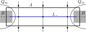
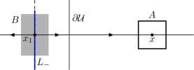
Case 2 Case 3

Figure 7. An illustration of Cases 2 and 3, with the flow lines of $\varphi^{t}$ drawn. The solid blue lines are $L_{-}$, the dashed lines containing them are $\{\rho=-\varepsilon\}$, and the semicircles denote $\operatorname{ell}_{h}(Q_{\infty})$. In this and the following figures, the elliptic sets of $B$ are shaded and $\operatorname{WF}_{h}(A)$ are pictured by the rectangles.

Case 3: $\operatorname{WF}_{h}(A)$ is contained in a small neighborhood of some $(x,\xi)\in\{\langle\xi\rangle^{-1}p=0\}$, where $x\in\overline{\mathcal{U}}\setminus\Gamma_{+}$. By (1.3), there exists $T>0$ such that $\varphi^{-T}(x)\notin\overline{\mathcal{U}}$. Similarly to the proof of Lemma 2.8, we use part 2 of Lemma 2.6 to see that $X_{1}\rho(\varphi^{-T}(x))>0$. We apply part 2 of Lemma 2.6 (with $[\alpha,\beta]=[-\varepsilon,0]$) again to see that there exists $T^{\prime}>0$ such that $x_{1}:=e^{-T^{\prime}X_{1}}(\varphi^{-T}(x))\in\{\rho=-\varepsilon\}\cap\{X_{1}\rho>0\}$ and $e^{-tX_{1}}(\varphi^{-T}(x))\in\{-\varepsilon<\rho<0\}$ for all $t\in[0,T^{\prime}]$. Since $X=\psi(\rho)X_{1}$, it follows that (see Figure 7)

$$\varphi^{-t}(x)\ \to\ x_{1}\in\{\rho=-\varepsilon\}\cap\{X_{1}\rho>0\}\quad\text{as }t\to+\infty.$$

By (4.24), there exists $B\in\Psi^{0}_{h}$ such that $\pi^{-1}(x_{1})\subset\operatorname{ell}_{h}(B)$ and $B\mathbf{u}$ is controlled either by Case 1 (if $\pi^{-1}(x_{1})\subset\operatorname{ell}_{h}(Q_{\infty})$) or by Case 2 (if $x_{1}\in L_{-}$). By propagation of singularities (Lemma 3.2) applied to $\mathbf{P}_{\delta,r}$, the estimate (4.26) holds for some $B_{1}\in\Psi^{0}_{h}$ microlocalized in a small neighborhood of $\{e^{-tH_{p}}(x,\xi)\mid t\geq 0\}$.

Case 4: $\operatorname{WF}_{h}(A)$ is contained in a small neighborhood $U$ of $\kappa(E_{s}^{*})$, where $\kappa$ is defined in (4.6); moreover, $\kappa(E_{s}^{*})\subset\operatorname{ell}_{h}(A)$. Take $B,B_{1}\in\Psi^{0}_{h}$ such that for some arbitrarily small fixed open sets $V\supset\kappa(E_{-}^{*})\cap\{\rho=\varepsilon\}$ and $W\supset\kappa(E_{-}^{*})$

$$\kappa(E_{-}^{*})\cap\{\rho=\varepsilon\}\ \subset\ \operatorname{ell}_{h}(B), \quad\operatorname{WF}_{h}(B)\ \subset\ V;$$

$$\kappa(E_{-}^{*})\ \subset\ \operatorname{ell}_{h}(B_{1}), \quad\operatorname{WF}_{h}(B_{1})\ \subset\ W;$$

see Figure 8. We also assume that (4.7) holds for the operators $A,B,B_{1}$.

We claim that for some choice of $U$ depending on $B,B_{1}$,

$$U\cap\{\langle\xi\rangle^{-1}p=0\}\setminus\pi^{-1}(\Gamma_{+})\ \subset\ \operatorname{Con}_{p}(\operatorname{ell}_{h}(B);\operatorname{ell}_{h}(B_{1})),$$ (4.28)

see Definition 3.1 for the notation on the right-hand side. To see (4.28), we first note that by Lemma 2.11, there exists $T^{\prime}\geq 0$ (depending on $B,B_{1}$, but not on $U$, as long as $U$ lies inside a fixed small neighborhood of $\kappa(E_{s}^{*})$) such that for each $T\geq T^{\prime}$ and each

$$(x,\xi)\in U\cap\{\langle\xi\rangle^{-1}p=0\},\quad\varphi^{-T}(x)\in\{\rho=\varepsilon\},$$ (4.29)

we have

$$e^{-TH_{p}}(x,\xi)\in\operatorname{ell}_{h}(B);\quad e^{-tH_{p}}(x,\xi)\in\operatorname{ell}_{h}(B_{1})\quad\text{for all }t\in[T^{\prime},T].$$ (4.30)

Since $\kappa(E_{s}^{*})$ is invariant under the flow and lies inside $\operatorname{ell}_{h}(B_{1})\setminus\{\rho=\varepsilon\}$, we can make sure that (4.29) never holds for $T\in[0,T^{\prime})$ and (4.30) holds for all $t\in[0,T]$, as long as $U$ is chosen small enough depending on $B,B_{1},T^{\prime}$. Now, for each $(x,\xi)\in U\cap\{\langle\xi\rangle^{-1}p=0\}\setminus\pi^{-1}(\Gamma_{+})$, there exists $T\geq 0$ such that (4.29) holds. Then (4.30) implies that $(x,\xi)\in\operatorname{Con}_{p}(\operatorname{ell}_{h}(B);\operatorname{ell}_{h}(B_{1}))$, which proves (4.28).

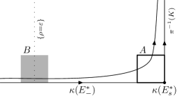
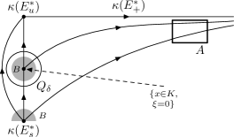
Case 4 Case 5

Figure 8. An illustration of Cases 4 and 5, with the flow lines of $e^{tH_{p}}$ drawn on $\overline{T}^{*}_{\Gamma_{-}}\mathcal{M}$ (Case 4) and $\overline{T}^{*}_{\Gamma_{+}}\mathcal{M}$ (Case 5). The right (Case 4) and left (Case 5) side of the pictures is $\pi^{-1}(K)$.

We now apply Lemma 3.7, with $\mathbf{P}=\mathbf{P}_{\delta}-z$, $L=\kappa(E_{s}^{*})$, $s=r$. To verify that $\operatorname{Im}\mathbf{P}\lesssim-h$ near $L$ on $H^{r}_{h}$, we use (4.20). By (4.28), we have $\Omega\cap\operatorname{WF}_{h}(A)\subset\pi^{-1}(\Gamma_{+})$. By Lemmas 2.3 and 2.11, we have $e^{-tH_{p}}(x,\xi)\to L$ as $t\to+\infty$ uniformly in $(x,\xi)\in\Omega\cap\operatorname{WF}_{h}(A)$. Finally, by (4.7), the space $H^{r}_{h}$ can be replaced by $\mathcal{H}^{r}_{h}$ in the estimate.

We see that (3.12) gives the estimate (4.26). By Lemma 2.2, $K\cap\{\rho=\varepsilon\}=\emptyset$ for $\varepsilon$ small enough; therefore we can choose $V$ so that $\pi(\operatorname{WF}_{h}(B))\subset\mathcal{U}\setminus\Gamma_{+}$. Then the term $B\mathbf{u}$ is controlled by Case 3.

Case 5: $\operatorname{WF}_{h}(A)$ is contained in a small neighborhood of some $(x,\xi)\in\{\langle\xi\rangle^{-1}p=0\}$, where $x\in\Gamma_{+}$ and $(x,\xi)\notin\kappa(E_{+}^{*})$. If $\xi\notin\overline{E_{+}^{*}(x)}$, then by part 4 of Lemma 2.10, we have $e^{-tH_{p}}(x,\xi)\to\kappa(E_{s}^{*})$ as $t\to+\infty$. Otherwise $\xi\in E_{+}^{*}(x)$ does not lie on the fiber infinity; by part 3 of Lemma 2.10, we have $e^{-tH_{p}}(x,\xi)\to\{x\in K,\ \xi=0\}$ as $t\to+\infty$.

Similarly to Case 3, we use propagation of singularities to obtain the estimate (4.26), where $B_{1}$ is microlocalized in a small neighborhood of $\{e^{-tH_{p}}(x,\xi)\mid t\geq 0\}$ and $\operatorname{WF}_{h}(B)$ lies either in a small neighborhood of $\kappa(E_{s}^{*})$ or in a small neighborhood of $\{x\in K,\ \xi=0\}$. In the first case, $B\mathbf{u}$ is controlled by Case 4; in the second case, $\operatorname{WF}_{h}(B)\subset\operatorname{ell}_{h}(Q_{\delta})$ and $B\mathbf{u}$ is controlled by Case 1. See Figure 8.

Case 6: $\operatorname{WF}_{h}(A)$ is contained in a small neighborhood $U$ of $\kappa(E_{u}^{*})$; moreover, $\kappa(E_{u}^{*})\subset\operatorname{ell}_{h}(A)$. Take $B\in\Psi^{0}_{h}$ such that (see Figure 9)

$$\kappa(E_{s}^{*})\cup\{x\in K,\ \xi=0\}\cup(\{\rho=\varepsilon\}\cap\pi^{-1}(\Gamma_{-}))\ \subset\ \operatorname{ell}_{h}(B)$$

and $\operatorname{WF}_{h}(B)$ lies in a small neighborhood of the above set. Let $B_{1}\in\Psi^{0}_{h}$ satisfy $\{\langle\xi\rangle^{-1}p=0\}\subset\operatorname{ell}_{h}(B_{1})$ and (4.19) hold near $\operatorname{WF}_{h}(B_{1})$. We claim that for $U$ small enough,

$$U\cap\{\langle\xi\rangle^{-1}p=0\}\setminus\kappa(E_{+}^{*})\ \subset\ \operatorname{Con}_{p}(\operatorname{ell}_{h}(B);\operatorname{ell}_{h}(B_{1})).$$ (4.31)

To show (4.31), take $(x,\xi)\in U\cap\{\langle\xi\rangle^{-1}p=0\}\setminus\kappa(E_{+}^{*})$. If $x\in\Gamma_{+}$, then by the analysis of Case 5, $(x,\xi)\in\operatorname{Con}_{p}(\operatorname{ell}_{h}(B);\operatorname{ell}_{h}(B_{1}))$. If $x\notin\Gamma_{+}$, then there exists $T>0$ such that $\varphi^{-T}(x)\in\{\rho=\varepsilon\}$; we claim that $\varphi^{-T}(x)\in\operatorname{ell}_{h}(B)$. Indeed, otherwise $\varphi^{-T}(x)$ does not lie in some fixed closed subset of $\overline{\mathcal{U}}$ which does not intersect $\Gamma_{-}$, which implies that $\varphi^{t-T}(x)\notin\pi(U)$ for $\pi(U)$ a small enough neighborhood of $K$ and all $t\geq 0$; putting $t:=T$, we get a contradiction.

We now apply Lemma 3.7 with $\mathbf{P}=\mathbf{P}_{\delta}-z$, $L=\kappa(E_{u}^{*})$, $s=-r$. To see that $\operatorname{Im}\mathbf{P}\lesssim-h$ near $L$ on $H^{-r}_{h}$, we use (4.21). By (4.31), $\Omega\cap\operatorname{WF}_{h}(A)\subset\kappa(E_{+}^{*})$. Then by Lemma 2.3 and the invariance of $E_{+}^{*}$ under the flow, $e^{-tH_{p}}(x,\xi)\to\kappa(E_{+}^{*})\cap\pi^{-1}(K)=\kappa(E_{u}^{*})$ as $t\to+\infty$ uniformly in $(x,\xi)\in\Omega\cap\operatorname{WF}_{h}(A)$.

By (3.12), we obtain (4.26). The space $H^{-r}_{h}$ can be replaced in (3.12) by $\mathcal{H}^{r}_{h}$; indeed, (3.24) still holds by (4.8) and (3.20), (3.21) follow by propagation of singularities for the conjugated operator $\mathbf{P}_{\delta,r}-z$. The term $B\mathbf{u}$ is controlled by Cases 1, 3, and 4, corresponding to the parts of $B$ lying near $\{x\in K,\ \xi=0\}$, $\{\rho=\varepsilon\}\cap\pi^{-1}(\Gamma_{-})$, and $\kappa(E_{s}^{*})$ respectively.

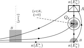
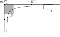
Case 6 Case 7

Figure 9. An illustration of Cases 6 and 7, with the flow lines of $e^{tH_{p}}$ drawn on $\overline{T}^{*}_{\Gamma_{-}}\mathcal{M}$ (Case 6) and $\overline{T}^{*}_{\Gamma_{+}}\mathcal{M}$ (Case 7).

Case 7: $\operatorname{WF}_{h}(A)$ is contained in a small neighborhood of some $(x,\xi)\in\kappa(E_{+}^{*})$. Take $B\in\Psi^{0}_{h}$ which is microlocalized in a small neighborhood of $\kappa(E_{u}^{*})$ and $\kappa(E_{u}^{*})\subset\operatorname{ell}_{h}(B)$. Let $B_{1}$ be as in Case 6. By Lemma 2.3 and the invariance of $E_{+}^{*}$, we see that $\operatorname{WF}_{h}(A)\subset\operatorname{Con}_{p}(\operatorname{ell}_{h}(B);\operatorname{ell}_{h}(B_{1}))$. Similarly to Case 3, propagation of singularities gives (4.26). The term $B\mathbf{u}$ is controlled by Case 6. See Figure 9.

Case 8: $\operatorname{WF}_{h}(A)$ is contained in a small neighborhood of some $(x,\xi)\in\{\langle\xi\rangle^{-1}p=0\}$ and $(x,\xi)\notin\operatorname{ell}_{h}(Q_{\infty})\cup\pi^{-1}(\overline{\mathcal{U}}\cup L_{-}\cup L_{+})$. Here $L_{\pm}$ are defined in (4.23). Then $x\in\{-2\varepsilon<\rho<0\}\setminus\{\rho=-\varepsilon\}$. By part 1 of Lemma 2.6 (with $[\alpha,\beta]=[-2\varepsilon,\varepsilon]$ or $[\alpha,\beta]=[-\varepsilon,0]$), and since $X=\psi(\rho)X_{1}$, $\operatorname{sgn}\psi(\rho)=\operatorname{sgn}(\rho+\varepsilon)$, we see that one of the following holds (see Figure 10)

1. there exists $T\geq 0$ such that $x_{1}:=\varphi^{-T}(x)\in\partial\overline{\mathcal{U}}$, or

2. there exists $T\geq 0$ such that $x_{1}:=\varphi^{-T}(x)\in\{\rho=-2\varepsilon\}$, or

3. there exists $x_{1}\in\{\rho=-\varepsilon\}\cap\{X_{1}\rho\geq 0\}$ such that $\varphi^{-t}(x)\to x_{1}$ as $t\to+\infty$.

Take $B\in\Psi^{0}_{h}$ such that $\pi^{-1}(x_{1})\in\operatorname{ell}_{h}(B)$, but $\pi(\operatorname{WF}_{h}(B))$ lies in a small neighborhood of $x_{1}$. Let $B_{1}$ be as in Case 6. Similarly to Case 3, by propagation of singularities we get (4.26). The term $B\mathbf{u}$ can be estimated in each of the situations above as follows:

1. by Cases 1, 3, 5, and 7;

2. by Case 1, since $\pi^{-1}(x_{1})\subset\operatorname{ell}_{h}(Q_{\infty})$;

3. by Case 2 if $x_{1}\in L_{-}$, and by Case 1 otherwise (as then $\pi^{-1}(x_{1})\subset\operatorname{ell}_{h}(Q_{\infty})$).

Case 9: $\operatorname{WF}_{h}(A)$ is contained in a small neighborhood of $\pi^{-1}(L_{+})$ and $\pi^{-1}(L_{+})\subset\operatorname{ell}_{h}(A)$, where $L_{+}$ is defined in (4.23). We in particular require that

$$\operatorname{WF}_{h}(A)\subset\textstyle\{-{3\over 2}\varepsilon<\rho<-{1\over 2}\varepsilon\}\cap\{X_{1}\rho<0\}.$$

Take $B\in\Psi^{0}_{h}$ such that (see Figure 10)

$$\begin{gathered}\operatorname{WF}_{h}(B)\ \subset\ \big{(}\{-2\varepsilon<\rho<0\}\cap\{\rho\neq-\varepsilon\}\big{)}\cup\operatorname{ell}_{h}(Q_{\infty}),\\ \pi^{-1}\big{(}\{\rho=-\varepsilon\}\cap\{X_{1}\rho\leq 0\}\setminus L_{+}^{\circ}\big{)}\ \subset\ \operatorname{ell}_{h}(B),\\ \textstyle\pi^{-1}\big{(}\{\rho=-{3\over 2}\varepsilon\}\cup\{\rho=-{1\over 2}\varepsilon\}\big{)}\ \subset\ \operatorname{ell}_{h}(B).\end{gathered}$$

We apply Lemma 3.7, with $\mathbf{P}=\mathbf{P}_{\delta,r}-z$, $L=\pi^{-1}(L_{+})$, $s=0$, and $B_{1}$ chosen as in Case 6. To verify that $\operatorname{Im}\mathbf{P}\lesssim-h$ near $L$ on $L^{2}$, we use (4.22). The condition $L\cap\operatorname{WF}_{h}(B)=\emptyset$ does not hold, but similarly to Case 2 it can be waived by taking a function $\chi\in C^{\infty}(\mathcal{M};[0,1])$ which is supported in a small enough neighborhood of $L_{+}$, but $\chi=1$ near $L_{+}$. As follows from the next paragraph, this function satisfies the conclusions of Lemma 3.8, in fact $H_{p}\chi=0$ near $\Omega$.

To finish verifying the assumptions of Lemma 3.7, note that $\operatorname{WF}_{h}(A)\cap\Omega\subset\pi^{-1}(L_{+}^{\circ})$. Indeed, let $(x,\xi)\in\operatorname{WF}_{h}(A)$. If $x\notin\{\rho=-\varepsilon\}$, then by part 1 of Lemma 2.6 (with $[\alpha,\beta]=[-{3\over 2}\varepsilon,-\varepsilon]$ or $[\alpha,\beta]=[-\varepsilon,-{1\over 2}\varepsilon]$), either $\varphi^{-T}(x)\in\{\rho=-{3\over 2}\varepsilon\}\cup\{\rho=-{1\over 2}\varepsilon\}$ for some $T\geq 0$, or $\varphi^{-t}(x)\to x_{1}\in\{\rho=-\varepsilon\}$ as $t\to+\infty$. The latter option is impossible if $\pi(\operatorname{WF}_{h}(A))$ is sufficiently close to $L_{+}\subset\{X_{1}\rho<0\}$, and the former option gives $(x,\xi)\notin\Omega$. If $x\in\{\rho=-\varepsilon\}$, then we also have $x\in\{X_{1}\rho<0\}$. Therefore, either $x\in L_{+}^{\circ}$ or $(x,\xi)\in\operatorname{ell}_{h}(B)$; in the latter case, $(x,\xi)\notin\Omega$.

Now, the estimate (3.12) gives (4.26). The term $B\mathbf{u}$ can be estimated by Cases 1 and 8.

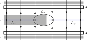
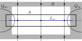
Case 8  Case 9

Figure 10. An illustration of Cases 8 and 9, with the flow lines of $\varphi^{t}$ drawn. The solid blue lines are $L_{\pm}$ and the dashed lines containing them are $\{\rho=-\varepsilon\}$; the solid lines on the top and bottom of Case 8 are $\partial\mathcal{U}$ and $\{\rho=-2\varepsilon\}$. The (semi)circles denote $\operatorname{ell}_{h}(Q_{\infty})$.

Combining the above cases and using a pseudodifferential partition of unity, we get the estimate (4.25). More precisely, if $A\in\Psi^{0}_{h}$ and $\operatorname{WF}_{h}(A)$ lies in a small neighborhood of $\pi^{-1}(\overline{\mathcal{U}})$, then $A\mathbf{u}$ is estimated by a combination of Cases 1, 3, 5, and 7. If $\pi^{-1}(\operatorname{WF}_{h}(A))\cap\overline{\mathcal{U}}=\emptyset$, then $A\mathbf{u}$ is estimated by a combination of Cases 1, 2, 8, and 9.

Reversing the direction of propagation (replacing $X_{1}$ by $-X_{1}$, $\mathbf{X}$ by $-\mathbf{X}$, $m$ by $-m$, and switching $E_{s}^{*}$ with $E_{u}^{*}$, $E_{+}^{*}$ with $E_{-}^{*}$, and $L_{+}$ with $L_{-}$), we repeat the above reasoning to get the adjoint estimate similar to [DyZw13, (3.17)]

$$\|\mathbf{u}\|_{\mathcal{H}^{-r}_{h}}\leq Ch^{-1}\|\mathbf{f}\|_{\mathcal{H}^{-r}_{h}},\quad\mathbf{u}\in\mathcal{H}^{-r}_{h},\quad\mathbf{f}:=(\mathbf{P}_{\delta}^{*}-\bar{z})\mathbf{u}\in\mathcal{H}^{-r}_{h}.$$ (4.32)

Note that $\mathcal{H}^{-r}_{h}$ is dual to $\mathcal{H}^{r}_{h}$ with respect to the $L^{2}$ pairing. The functional analytic argument given at the end of the proof of [DyZw13, Proposition 3.4] shows that together, (4.25) and (4.32) imply invertibility of $\mathbf{P}_{\delta}-z:\mathcal{D}^{r}_{h}\to\mathcal{H}^{r}_{h}$ and the bound (4.13).

It remains to verify the wavefront set condition (4.14). By [DyZw13, Lemma 2.3], it suffices to show that for each $(x,\xi),(y,\eta)\in T^{*}\mathcal{U}$ such that $(y,\eta)\neq(x,\xi)$ and either $p(x,\xi)\neq 0$ or $(x,\xi)\neq e^{tH_{p}}(y,\eta)$ for all $t\geq 0$, there exist $A\in\Psi^{\operatorname{comp}}_{h}(\mathcal{M})$ and $B_{2}\in\Psi^{0}_{h}(\mathcal{M})$ such that

$$(x,\xi)\in\operatorname{ell}_{h}(A),\ (y,\eta)\notin\operatorname{WF}_{h}(B_{2}),$$

and for each $\mathbf{u}\in\mathcal{D}^{r}_{h}$ with $\mathbf{f}:=(\mathbf{P}_{\delta}-z)\mathbf{u}$,

$$\|A\mathbf{u}\|_{\mathcal{H}^{r}_{h}}\leq Ch^{-1}\|B_{2}\mathbf{f}\|_{\mathcal{H}^{r}_{h}}+\mathcal{O}(h^{\infty})\|\mathbf{u}\|_{\mathcal{H}^{r}_{h}}.$$ (4.33)

As remarked after (4.25), an approximation argument reduces us to the case $\mathbf{u}\in C^{\infty}$. Then (4.33) follows by a combination of Cases 1, 3, and 5. Here we use that the operator $B_{1}$ from Case 2 is microlocalized in a small neighborhood of $\pi^{-1}(L_{-})\subset\pi^{-1}(\mathcal{M}\setminus\mathcal{U})$ and the same operator from Case 4 is microlocalized in a small neighborhood of $\kappa(E_{-}^{*})\subset\partial\overline{T}^{*}\mathcal{M}$; thus their wavefront sets do not contain $(y,\eta)$. ∎

4.2. Proofs of Theorems 1 and 2

In this section, we show the meromorphic continuation of the resolvent $\mathbf{R}(\lambda)$ defined in (1.11). We start with the following corollary of Lemma 4.2:

Lemma 4.3.

Let $Q_{\infty}\in\Psi^{1}_{h}(\mathcal{M}),Q_{\delta}\in\Psi^{\operatorname{comp}}_{h}(\mathcal{M}),q_{1}\in C^{\infty}(\mathcal{M})$ be introduced in (4.9), and $\mathcal{H}^{r}_{h},\mathcal{D}^{r}_{h}$ be given by (4.4), (4.11). Fix $C_{1},C_{2}>0$ and $r>r_{0}=r_{0}(C_{1})$. Define

$$\mathbf{P}_{0}=\mathbf{P}_{0}(h):={h\over i}\mathbf{X}-i(Q_{\infty}+q_{1}):\mathcal{D}^{r}_{h}\to\mathcal{H}^{r}_{h}.$$ (4.34)

Then for $0<h<h_{0}(C_{1},C_{2},r)$,

1. $\mathbf{P}_{0}-z:\mathcal{D}^{r}_{h}\to\mathcal{H}^{r}_{h}$ is a Fredholm operator of index zero for $z\in[-C_{2}h,C_{2}h]+i[-C_{1}h,1]$.

2. The inverse

$$\mathbf{R}_{0}(z):=(\mathbf{P}_{0}-z)^{-1}:\mathcal{H}^{r}_{h}\to\mathcal{D}^{r}_{h},\quad z\in[-C_{2}h,C_{2}h]+i[-C_{1}h,1]$$ (4.35)

is a meromorphic family of operators with poles of finite rank.

Proof.

1. Take $z\in[-C_{2}h,C_{2}h]+i[-C_{1}h,1]$. By Lemma 4.2, $\mathbf{P}_{\delta}-z:\mathcal{D}^{r}_{h}\to\mathcal{H}^{r}_{h}$ is invertible, where $\mathbf{P}_{\delta}$ is defined in (4.10). We write

$$\mathbf{P}_{\delta}-z=\mathbf{P}_{0}-z-iQ_{\delta}.$$

Now, $Q_{\delta}$ is compactly microlocalized (that is, $\operatorname{WF}_{h}(Q_{\delta})\Subset T^{*}\mathcal{M}$) so it is smoothing; that is, $Q_{\delta}$ is bounded $H^{-N}(\mathcal{M})\to H^{N}(\mathcal{M})$ for all $N$. By Rellich’s Theorem (using the fact that $\mathcal{M}$ is compact and $e^{\pm rG}$ are pseudodifferential operators), we see that $Q_{\delta}$ is a compact operator $\mathcal{H}^{r}_{h}\to\mathcal{H}^{r}_{h}$ and thus $\mathcal{D}^{r}_{h}\to\mathcal{H}^{r}_{h}$. It follows that $\mathbf{P}_{0}-z:\mathcal{D}^{r}_{h}\to\mathcal{H}^{r}_{h}$ is a Fredholm operator of index zero.

2. The meromorphy of $\mathbf{R}_{0}(z)$ follows by analytic Fredholm theory [Zw, Proposition D.4], as long as $\mathbf{P}_{0}-z$ is known to be invertible for at least one value of $z$. We take $z=i$; it suffices to prove the estimate

$$\|\mathbf{u}\|_{\mathcal{H}^{r}_{h}}\leq Ch^{-1}\|\mathbf{f}\|_{\mathcal{H}^{r}_{h}},\quad\mathbf{u}\in\mathcal{D}^{r}_{h},\quad\mathbf{f}=(\mathbf{P}_{0}-i)\mathbf{u}.$$ (4.36)

Similarly to (4.17), let $\mathbf{P}_{0,r}:=e^{rG}\mathbf{P}_{0}e^{-rG}\in\Psi^{1}_{h}(\mathcal{M};\mathcal{E})$. Note that $\operatorname{Im}\sigma_{h}(\mathbf{P}_{0,r})\leq 0$ near $\{\langle\xi\rangle^{-1}p=0\}$ and $\operatorname{Re}\sigma_{h}(\mathbf{P}_{0,r})=p$ similarly to (4.18), (4.19). By (4.4) and the approximation argument following (4.25), we reduce (4.36) to

$$\|\mathbf{v}\|_{L^{2}}\leq Ch^{-1}\|\mathbf{g}\|_{L^{2}},\quad\mathbf{v}\in C^{\infty}(\mathcal{M};\mathcal{E}),\quad\mathbf{g}=(\mathbf{P}_{0,r}-i)\mathbf{v}.$$ (4.37)

We now apply Lemma 3.7, with $\mathbf{P}=\mathbf{P}_{0,r}-i$, $L=\{\langle\xi\rangle^{-1}p=0\}$, $s=0$, and $B=0$. Note that $\operatorname{Im}\mathbf{P}\lesssim-h$ on $L^{2}$ near $L$ by Lemma 3.5, with $Q:=1$. By (3.12), we get for some $A,B_{1}\in\Psi^{0}$ such that $\{\langle\xi\rangle^{-1}p=0\}\subset\operatorname{ell}_{h}(A)$ and $B_{1}$ is microlocalized in a neighborhood of $\{\langle\xi\rangle^{-1}p=0\}$,

$$\|A\mathbf{v}\|_{L^{2}}\leq Ch^{-1}\|B_{1}\mathbf{g}\|_{L^{2}}+\mathcal{O}(h^{\infty})\|\mathbf{v}\|_{L^{2}}.$$

Combining this with the elliptic estimate (4.27) valid for $\operatorname{WF}_{h}(A)\cap\{\langle\xi\rangle^{-1}p=0\}=\emptyset$, we get (4.37). ∎

The operator $\mathbf{R}_{0}(z)$ depends on the choice of $Q_{\infty},q_{1}$ (and thus on $h$). It is independent of the choice of $r$, but proving this would require a separate argument. However, the restriction of this operator to $\mathcal{U}$ is independent of $Q_{\infty},q_{1},r$. This is a byproduct of the following

Lemma 4.4.

In the notation of Lemma 4.3, let $\lambda\in[-C_{1},h^{-1}]+i[-C_{2},C_{2}]$ and put $z:=ih\lambda$. Assume also that $\operatorname{Re}\lambda>C_{0}$, where $C_{0}$ is defined in (1.9). Then

$$\mathbf{R}(\lambda)\mathbf{f}=-ih\mathbf{R}_{0}(z)\mathbf{f}|_{\mathcal{U}}\quad\text{for all}\quad\mathbf{f}\in C_{0}^{\infty}(\mathcal{U};\mathcal{E}).$$ (4.38)

Proof.

By analyticity and since $h$ can be chosen arbitrarily small, it suffices to prove (4.38) in the case $\operatorname{Re}\lambda>C_{3}$, where $C_{3}>C_{0}$ is a large enough constant depending on $r$, but not on $h$. As discussed after (4.4), the anisotropic Sobolev space $\mathcal{H}^{r}_{h}$ contains the standard Sobolev space $H^{N}_{h}(\mathcal{M};\mathcal{E})$, for $N$ large enough depending on $r$.

We consider an extension of $\mathbf{X}$ to $\mathcal{M}$ such that (1.6) holds on $\mathcal{M}$. Note that (1.6) holds also for the operator $\mathbf{X}+h^{-1}q_{1}$, since $q_{1}\in C^{\infty}(\mathcal{M})$ is a multiplication operator. We claim that for some $C_{3}$ depending on $N$, but not on $h$,

$$\|e^{-t(\mathbf{X}+h^{-1}q_{1})}\mathbf{f}\|_{H^{N}_{h}}\leq C(h)e^{C_{3}t},\quad t\geq 0.$$ (4.39)

This follows by writing the transfer operator $e^{-t(\mathbf{X}+h^{-1}q_{1})}$ in the form similar to (1.7) using a local trivialization of the bundle $\mathcal{E}$, with $V$ now a matrix. Here we use the fact that each derivative of $\varphi^{-t}$ is bounded exponentially in $t$. The term $h^{-1}q_{1}$ does not change the value of $C_{3}$, as $q_{1}\geq 0$ everywhere and $t\geq 0$, see (1.7).

Now, for $\operatorname{Re}\lambda>C_{3}$ and $z:=ih\lambda$ not a pole of $\mathbf{R}_{0}$, consider the function

$$\mathbf{v}:=\int_{0}^{\infty}e^{-t(\mathbf{X}+h^{-1}q_{1}+\lambda)}\mathbf{f}\,dt\ \in\ H^{N}_{h}(\mathcal{M};\mathcal{E})\ \subset\ \mathcal{H}^{r}_{h}.$$

Since $\operatorname{supp}\mathbf{f}\subset\mathcal{U}$, $\operatorname{supp}q_{1}\cap\overline{\mathcal{U}}=\emptyset$, and $\mathcal{U}$ is convex, it follows that (see (1.7))

$$\mathbf{R}(\lambda)\mathbf{f}=\mathbf{v}\quad\text{on }\mathcal{U}.$$ (4.40)

We also have $\operatorname{supp}\mathbf{v}\subset\overline{\Sigma}$, where $\Sigma$ is defined in (2.4). (In fact, (1.8) implies that $\operatorname{supp}\mathbf{v}\subset\overline{\Sigma_{+}}$.) Therefore, $Q_{\infty}\mathbf{v}=0$. It follows that

$$(\mathbf{P}_{0}-z)\mathbf{v}=-ih\mathbf{f},\quad\mathbf{v}\in\mathcal{D}^{r}_{h}.$$

Since $\mathbf{P}_{0}-z$ is invertible $\mathcal{D}^{r}_{h}\to\mathcal{H}^{r}_{h}$, we have

$$-ih\mathbf{R}_{0}(z)\mathbf{f}=\mathbf{v}.$$ (4.41)

Combining (4.40) and (4.41), we get (4.38). ∎

Proof of Theorem 1.

By Lemmas 4.3 and 4.4, the operator $-ih\operatorname{1\hskip-2.75ptl}_{\mathcal{U}}\mathbf{R}_{0}(ih\lambda)\operatorname{1\hskip-2.75ptl}_{\mathcal{U}}$ gives the meromorphic continuation of $\mathbf{R}(\lambda)$ in the region $[-C_{1},h^{-1}]+i[-C_{2},C_{2}]$ for $h$ small enough. Since $C_{1},C_{2}$ can be chosen arbitrarily and $h$ can be arbitrarily small, we obtain the continuation to the entire complex plane. ∎

Note that for all $\lambda\in\mathbb{C}$,

$$(\mathbf{X}+\lambda)\mathbf{R}(\lambda)=\mathbf{R}(\lambda)(\mathbf{X}+\lambda)=1\ :\ C_{0}^{\infty}(\mathcal{U})\to\mathcal{D}^{\prime}(\mathcal{U}).$$ (4.42)

Indeed, by analytic continuation it suffices to consider the case $\operatorname{Re}\lambda>C_{0}$; in this case, (4.42) follows from (1.10).

The following microlocalization statement is used in the proofs of Theorems 2 and 3. See (3.1) and (3.2) for the notation used below.

Lemma 4.5.

Let $\lambda_{0}\in\mathbb{C}$. Then the expansion (1.13) holds for $\mathbf{R}_{H}(\lambda):C_{0}^{\infty}(\mathcal{U};\mathcal{E})\to\mathcal{D}^{\prime}(\mathcal{U};\mathcal{E})$ holomorphic near $\lambda_{0}$ and a finite rank operator $\Pi=\Pi_{\lambda_{0}}:C_{0}^{\infty}(\mathcal{U};\mathcal{E})\to\mathcal{D}^{\prime}(\mathcal{U};\mathcal{E})$. Moreover, $\operatorname{supp}K_{\Pi}\subset\Gamma_{+}\times\Gamma_{-}$ and

$$\operatorname{WF}^{\prime}(\mathbf{R}_{H}(\lambda))\ \subset\ \Delta(T^{*}\mathcal{U})\cup\Upsilon_{+}\cup(E_{+}^{*}\times E_{-}^{*}),\quad\operatorname{WF}^{\prime}(\Pi)\ \subset\ E_{+}^{*}\times E_{-}^{*},$$ (4.43)

where $\Delta(T^{*}\mathcal{U})$ is the diagonal, $E_{\pm}^{*}\subset T^{*}\overline{\mathcal{U}}$ are defined in Lemma 2.10, and

$$\Upsilon_{+}=\{(e^{tH_{p}}(y,\eta),y,\eta)\mid t\geq 0,\ p(y,\eta)=0,\ y\in\mathcal{U},\ \varphi^{t}(y)\in\mathcal{U}\}.$$

Proof.

We argue similarly to the proof of [DyZw13, Proposition 3.3]. By Theorem 1,

$$\mathbf{R}(\lambda)=\mathbf{R}_{H}(\lambda)+\sum_{j=1}^{J(\lambda_{0})}{\mathbf{A}_{j}\over(\lambda-\lambda_{0})^{j}}$$ (4.44)

where $\mathbf{R}_{H}(\lambda):C_{0}^{\infty}(\mathcal{U};\mathcal{E})\to\mathcal{D}^{\prime}(\mathcal{U};\mathcal{E})$ is holomorphic near $\lambda_{0}$ and $\mathbf{A}_{j}:C_{0}^{\infty}(\mathcal{U};\mathcal{E})\to\mathcal{D}^{\prime}(\mathcal{U};\mathcal{E})$ are finite rank operators. Plugging this expansion into (4.42), we get

$$\mathbf{A}_{j+1}=-(\mathbf{X}+\lambda_{0})\mathbf{A}_{j},\ 1\leq j<J(\lambda_{0});\quad(\mathbf{X}+\lambda_{0})\mathbf{A}_{J(\lambda_{0})}=0.$$ (4.45)

The expansion (1.13) follows from here by putting $\Pi:=\mathbf{A}_{1}$.

If $\psi_{1},\psi_{2}\in C_{0}^{\infty}(\mathcal{U})$ satisfy $\operatorname{supp}\psi_{1}\cap\Gamma_{-}=\operatorname{supp}\psi_{2}\cap\Gamma_{+}=\emptyset$, then Lemma 2.9 shows that $\mathbf{R}(\lambda)\psi_{1},\psi_{2}\mathbf{R}(\lambda)$ are holomorphic for all $\lambda\in\mathbb{C}$. Therefore, $\Pi\psi_{1}=\psi_{2}\Pi=0$; this implies that $\operatorname{supp}K_{\Pi}\subset\Gamma_{+}\times\Gamma_{-}$.

We finally prove (4.43). We start by writing the following identity relating the auxiliary resolvents defined by (4.12) and (4.35) (we put $z:=ih\lambda$):

$$\mathbf{R}_{0}(z)=\mathbf{R}_{\delta}(z)-i\mathbf{R}_{\delta}(z)Q_{\delta}\mathbf{R}_{\delta}(z)-\mathbf{R}_{\delta}(z)Q_{\delta}\mathbf{R}_{0}(z)Q_{\delta}\mathbf{R}_{\delta}(z).$$

Since $Q_{\delta}$ is supported inside $\mathcal{U}$, by (4.38) this gives

$$\mathbf{R}(\lambda)=-ih\operatorname{1\hskip-2.75ptl}_{\mathcal{U}}\big{(}\mathbf{R}_{\delta}(z)-i\mathbf{R}_{\delta}(z)Q_{\delta}\mathbf{R}_{\delta}(z)\big{)}\operatorname{1\hskip-2.75ptl}_{\mathcal{U}}-\operatorname{1\hskip-2.75ptl}_{\mathcal{U}}\mathbf{R}_{\delta}(z)Q_{\delta}\mathbf{R}(\lambda)Q_{\delta}\mathbf{R}_{\delta}(z)\operatorname{1\hskip-2.75ptl}_{\mathcal{U}}.$$ (4.46)

We analyse each of the terms on the right-hand side separately. By (4.14), we have

$$\operatorname{WF}_{h}^{\prime}(\mathbf{R}_{\delta}(z))\cap T^{*}(\mathcal{U}\times\mathcal{U})\ \subset\ \Delta(T^{*}\mathcal{U})\cup\Upsilon_{+}.$$ (4.47)

By (3.3), and since $\operatorname{WF}_{h}(Q_{\delta})\subset T^{*}\mathcal{U}$, we get

$$\operatorname{WF}_{h}^{\prime}(\mathbf{R}_{\delta}(z)Q_{\delta}\mathbf{R}_{\delta}(z))\cap T^{*}(\mathcal{U}\times\mathcal{U})\ \subset\ \Delta(T^{*}\mathcal{U})\cup\Upsilon_{+}.$$

To handle the third term in (4.46), note that for each family of operators $\mathbf{T}(\lambda):C_{0}^{\infty}(\mathcal{U};\mathcal{E})\to\mathcal{D}^{\prime}(\mathcal{U};\mathcal{E})$ which is holomorphic in $\lambda$ and independent of $h$, we have by (3.3)

$$\begin{gathered}\operatorname{WF}_{h}^{\prime}(\mathbf{R}_{\delta}(z)Q_{\delta}\mathbf{T}(\lambda)Q_{\delta}\mathbf{R}_{\delta}(z))\cap T^{*}(\mathcal{U}\times\mathcal{U})\ \subset\ \Theta_{\delta}^{+}\times\Theta_{\delta}^{-},\\ \Theta_{\delta}^{\pm}=T^{*}\mathcal{U}\cap\bigcup_{\pm t\geq 0}e^{tH_{p}}(\operatorname{WF}_{h}(Q_{\delta})).\end{gathered}$$

Plugging the expansion (1.13) into the third term in (4.46) and using that the terms in this expansion are $h$-independent and $\mathbf{R}(\lambda)$ does not depend on $\delta$, we get

$$\operatorname{WF}_{h}^{\prime}(\mathbf{R}_{H}(\lambda))\cap T^{*}(\mathcal{U}\times\mathcal{U}) \subset\ \Delta(T^{*}\mathcal{U})\cup\Upsilon_{+}\cup\Big{(}\bigcap_{\delta}\Theta_{\delta}^{+}\times\bigcap_{\delta}\Theta_{\delta}^{-}\Big{)},$$

$$\operatorname{WF}_{h}^{\prime}(\Pi)\cap T^{*}(\mathcal{U}\times\mathcal{U}) \subset\ \bigcap_{\delta}\Theta_{\delta}^{+}\times\bigcap_{\delta}\Theta_{\delta}^{-}.$$

Since $\mathbf{R}_{H}(\lambda)$ is independent of $h$, by [DyZw13, (2.6)] we have

$$\operatorname{WF}^{\prime}(\mathbf{R}_{H}(\lambda))=\operatorname{WF}_{h}^{\prime}(\mathbf{R}_{H}(\lambda))\cap(T^{*}(\mathcal{U}\times\mathcal{U})\setminus 0),$$

and same is true for $\Pi$. To show (4.43), it remains to prove that

$$\bigcap_{\delta}\Theta_{\delta}^{\pm}\subset E_{\pm}^{*}.$$

Take $(y,\eta)\in\bigcap_{\delta}\Theta_{\delta}^{\pm}$. By taking a sequence of $\delta$ converging to 0, we see that there exists a sequence $t_{j}$ such that $e^{\mp t_{j}H_{p}}(y,\eta)\to\{x\in K,\ \xi=0\}$. If $y\notin\Gamma_{\pm}$, then the trajectory $\{\varphi^{\mp t}(y)\mid t\geq 0\}$ never passes through some neighborhood of $K$; therefore, we have $y\in\Gamma_{\pm}$. Since $p$ is preserved along the trajectories of $e^{tH_{p}}$, we have $p(y,\eta)=0$. Finally, if $\eta\notin E_{\pm}^{*}(y)$, then by part 4 of Lemma 2.10 the trajectory $\{e^{\mp tH_{p}}(y,\eta)\mid t\geq 0\}$ never passes through some neighborhood of the zero section and we have a contradiction. It follows that $(y,\eta)\in E_{\pm}^{*}$ as required. ∎

For the proof of Theorem 2, we also need

Lemma 4.6.

Assume that $\mathbf{u}\in\mathcal{D}^{\prime}(\mathcal{U};\mathcal{E})$ satisfies

$$\operatorname{supp}\mathbf{u}\ \subset\ \Gamma_{+},\quad\operatorname{WF}(\mathbf{u})\ \subset\ E_{+}^{*}.$$ (4.48)

For some $\lambda\in\mathbb{C}$, put $\mathbf{f}:=(\mathbf{X}+\lambda)\mathbf{u}$. Take $\chi,\chi^{\prime}\in C_{0}^{\infty}(\mathcal{U})$ satisfying (2.3) and $\chi=1$ near $K$. Then:

1. For $r>0$ large enough, $\chi^{\prime}\mathbf{u}$ and $\chi^{\prime}\mathbf{f}$ lie in the space $\mathcal{H}^{r}_{h}$ from (4.4). By Lemmas 4.3 and 4.4, this makes it possible to define $\mathbf{R}(\lambda)\chi^{\prime}\mathbf{f}\in\mathcal{D}^{\prime}(\mathcal{U};\mathcal{E})$.

2. We have $\chi\mathbf{u}=\chi\mathbf{R}(\lambda)\chi^{\prime}\mathbf{f}$.

Proof.

1. Take $r>0$ large enough so that $\chi^{\prime}\mathbf{u}\in H^{-r}_{h}(\mathcal{M};\mathcal{E})$. By Lemma 4.1, the order function $m$ is equal to $-1$ near $E_{+}^{*}\supset\operatorname{WF}(\chi^{\prime}\mathbf{u})$. Let $G=G(h)$ be the operator defined in (4.2). Then $e^{rG(h)}$ is a nonsemiclassical pseudodifferential operator of order $-r$ microlocally near $\operatorname{WF}(\chi^{\prime}\mathbf{u})$. It follows that $e^{rG(h)}\chi^{\prime}\mathbf{u}\in L^{2}$ and thus $\chi^{\prime}\mathbf{u}\in\mathcal{H}^{r}_{h}$. Since $\mathbf{f}$ satisfies (4.48) as well, we similarly have $\chi^{\prime}\mathbf{f}\in\mathcal{H}^{r}_{h}$.

2. Since $\chi^{\prime}\mathbf{u}\in\mathcal{H}^{r}_{h}$ and $\mathbf{X}\chi^{\prime}\mathbf{u}\in\mathcal{H}^{r}_{h}$ for $r$ large enough, we have by Lemmas 4.3 and 4.4,

$$\chi\mathbf{u}=\chi\chi^{\prime}\mathbf{u}=\chi\mathbf{R}(\lambda)(\mathbf{X}+\lambda)\chi^{\prime}\mathbf{u}.$$

Now, by (1.6)

$$(\mathbf{X}+\lambda)\chi^{\prime}\mathbf{u}=(X\chi^{\prime})\mathbf{u}+\chi^{\prime}\mathbf{f}.$$

Take $x\in\Gamma_{+}\cap\operatorname{supp}(X\chi^{\prime})$. By Lemma 2.3, there exists $t^{\prime}>0$ such that $\varphi^{-t^{\prime}}(x)\in\operatorname{supp}\chi$. Then by (2.3), $\varphi^{t}(x)\notin\operatorname{supp}\chi$ for all $t\geq 0$. In particular, $x\notin\Gamma_{-}$. Since $\operatorname{supp}\mathbf{u}\subset\Gamma_{+}$, there exists $\psi_{1}\in C_{0}^{\infty}(\mathcal{M})$ such that $(X\chi^{\prime})\mathbf{u}=\psi_{1}(X\chi^{\prime})\mathbf{u}$ and $\operatorname{supp}\psi_{1}\cap\Gamma_{-}=\emptyset$. Then $\mathbf{R}(\lambda)\psi_{1}$ is given by (2.7). It follows from (1.8) that

$$\chi\mathbf{R}(\lambda)(X\chi^{\prime})\mathbf{u}=0$$

and thus $\chi\mathbf{u}=\chi\mathbf{R}(\lambda)\chi^{\prime}\mathbf{f}$ as needed. ∎

Proof of Theorem 2.

The expansion (1.13) and the properties (1.14) have already been established in Lemma 4.5. Therefore, it remains to prove (1.15). The property $\mathbf{X}\Pi=\Pi\mathbf{X}$ follows from (1.13) and (4.42). By (1.14) and (4.45), we know that

$$\operatorname{Ran}\Pi\ \subset\ \operatorname{Res}^{(J(\lambda_{0}))}_{\mathbf{X}}(\lambda_{0}),$$

therefore it remains to prove that for each $N$,

$$\mathbf{u}\in\operatorname{Res}^{(N)}_{\mathbf{X}}(\lambda_{0})\ \Longrightarrow\ \mathbf{u}=\Pi\mathbf{u}.$$ (4.49)

Take $\chi\in C_{0}^{\infty}(\mathcal{U})$ such that $\chi=1$ near $K$ and let $\chi^{\prime}\in C_{0}^{\infty}(\mathcal{U})$ be constructed in Lemma 2.5. We claim that for each $j=0,\dots,N$,

$$\chi\mathbf{R}(\lambda)\chi^{\prime}(\mathbf{X}+\lambda_{0})^{j}\mathbf{u}=\sum_{k=j}^{N-1}{(-1)^{k-j}\chi(\mathbf{X}+\lambda_{0})^{k}\mathbf{u}\over(\lambda-\lambda_{0})^{k-j+1}}.$$ (4.50)

We argue by induction on $j=N,\dots,0$. For $j=N$, we have $(\mathbf{X}+\lambda_{0})^{j}\mathbf{u}=0$ and (4.50) is trivial. Now, assume that (4.50) is true for $j+1$. Using the identity

$$(\mathbf{X}+\lambda_{0})^{j}\mathbf{u}={(\mathbf{X}+\lambda)(\mathbf{X}+\lambda_{0})^{j}\mathbf{u}-(\mathbf{X}+\lambda_{0})^{j+1}\mathbf{u}\over\lambda-\lambda_{0}}$$

and Lemma 4.6 for the first term on the right-hand side, we obtain (4.50) for $j$, finishing its proof.

Now, take $j=0$ in (4.50) and use (1.13). Equating the terms next to $(\lambda-\lambda_{0})^{-1}$, we obtain $\chi\mathbf{u}=\chi\Pi\chi^{\prime}\mathbf{u}$. Moreover, $\Pi\chi^{\prime}\mathbf{u}=\Pi\mathbf{u}$ since $\operatorname{supp}K_{\Pi}\subset\Gamma_{+}\times\Gamma_{-}$, $\operatorname{supp}\mathbf{u}\subset\Gamma_{+}$, and $\chi^{\prime}=1$ near $K$. Since $\chi$ could be chosen arbitrarily, this gives (4.49). ∎

5. Dynamical traces and zeta functions

In this section we prove Theorem 3. More generally, we prove in Theorem 4 below that the dynamical trace $F_{\mathbf{X}}(\lambda)$ associated to $\mathbf{X}$ is equal to the flat trace of a certain operator featuring the resolvent $\mathbf{R}(\lambda)$; this flat trace gives the meromorphic extension of $F_{\mathbf{X}}(\lambda)$. The key ingredient of the proof is the wavefront set condition (4.43) on the meromorphic extension of the resolvent. We follow the strategy of [DyZw13] and refer the reader to that paper for the parts of the proof that remain unchanged in our more general case.

5.1. Meromorphic extension of traces

We first show how to express Pollicott–Ruelle resonances of $\mathbf{X}$ as the poles of a certain trace expression featuring closed geodesics. To write down this expression, we need to introduce some notation. Define the vector bundle $\mathcal{E}_{0}$ over $\overline{\mathcal{U}}$ by

$$\mathcal{E}_{0}(x)=\{\eta\in T^{*}_{x}\mathcal{M}\mid\langle X(x),\eta\rangle=0\},\quad x\in\overline{\mathcal{U}}.$$ (5.1)

Assume that $x,\varphi^{t}(x)\in\mathcal{U}$ for some $t$. Define the linearized Poincaré map

$$\mathcal{P}_{x,t}:\mathcal{E}_{0}(x)\to\mathcal{E}_{0}(\varphi^{t}(x)),\quad\mathcal{P}_{x,t}=(d\varphi^{t}(x))^{-T}|_{\mathcal{E}_{0}(x)}.$$

Here $(d\varphi^{t}(x))^{-T}$ is the inverse transpose of $d\varphi^{t}(x)$ as in (2.9). Next, the parallel transport

$$\alpha_{x,t}:\mathcal{E}(x)\to\mathcal{E}(\varphi^{t}(x))$$

is defined as follows: for each $\mathbf{u}\in C^{\infty}(\mathcal{M};\mathcal{E})$, we put $\alpha_{x,t}(\mathbf{u}(x))=e^{-t\mathbf{X}}\mathbf{u}(\varphi^{t}(x))$. This definition only depends on the value of $\mathbf{u}$ at $x$; indeed, (1.8) shows that if $\mathbf{u}(x)=0$, then $e^{-t\mathbf{X}}\mathbf{u}(\varphi^{t}(x))=0$ as well (by writing $\mathbf{u}$ as a sum of expressions of the form $f\mathbf{v}$, where $f\in C^{\infty}(\mathcal{M})$ vanish at $x$).

Now, assume that $\gamma(t)=\varphi^{t}(x_{0})$ is a closed trajectory, that is $\gamma(T)=\gamma(0)$ for some $T>0$. (We call $T$ the period of $\gamma$, and regard the same $\gamma$ with two different values of $T$ as two different closed trajectories. The minimal positive $T^{\sharp}$ such that $\gamma(T^{\sharp})=\gamma(0)$ is called the primitive period.) Assume also that $x_{0}\in\mathcal{U}$; this implies immediately that $\gamma$ lies inside $K$. The operators $\alpha_{\gamma(t),T}:\mathcal{E}(\gamma(t))\to\mathcal{E}(\gamma(t))$, as well as $\mathcal{P}_{\gamma(t),T}:\mathcal{E}_{0}(\gamma(t))\to\mathcal{E}_{0}(\gamma(t))$, are conjugate to each other for different $t$, therefore the trace and the determinant

$$\operatorname{tr}\alpha_{\gamma}:=\operatorname{tr}\alpha_{\gamma(t),T},\quad\det(I-\mathcal{P}_{\gamma}):=\det(I-\mathcal{P}_{\gamma(t),T})$$ (5.2)

do not depend on $t$. Note that by (2.11),

$$\det(I-\mathcal{P}_{\gamma})\neq 0.$$ (5.3)

The main result of this subsection, and the key ingredient for showing meromorphic continuation of dynamical zeta functions, is

Theorem 4.

Define for $\operatorname{Re}\lambda\gg 1$,

$$F_{\mathbf{X}}(\lambda):=\sum_{\gamma}{e^{-\lambda T_{\gamma}}\,T_{\gamma}^{\sharp}\,\operatorname{tr}\alpha_{\gamma}\over|\det(I-\mathcal{P}_{\gamma})|}$$ (5.4)

where the sum is over all closed trajectories $\gamma$ inside $K$, $T_{\gamma}>0$ is the period of $\gamma$, and $T_{\gamma}^{\sharp}$ is the primitive period. Then $F(\lambda)$ extends meromorphically to $\lambda\in\mathbb{C}$. The poles of $F(\lambda)$ are the Pollicott–Ruelle resonances of $\mathbf{X}$ and the residue at a pole $\lambda_{0}$ is equal to the rank of $\Pi_{\lambda_{0}}$ (see Theorem 2).

Remark. The sum (5.4) converges for large $\operatorname{Re}\lambda$, since $|\det(I-\mathcal{P}_{\gamma})|$ is bounded away from zero, $\alpha_{\gamma}$ grows at most exponentially in $T_{\gamma}$, and the number of closed trajectories grows at most exponentially by Lemma 2.17.

Proof.

We use the concept of the flat trace of an operator $\mathbf{A}:C^{\infty}(\mathcal{M};\mathcal{U})\to\mathcal{D}^{\prime}(\mathcal{M};\mathcal{U})$ satisfying the condition

$$\operatorname{WF}^{\prime}(\mathbf{A})\cap\Delta(T^{*}\mathcal{M}\setminus 0)=\emptyset,\quad\Delta(T^{*}\mathcal{M}\setminus 0)=\{(x,\xi,x,\xi)\mid(x,\xi)\in T^{*}\mathcal{M}\setminus 0\}.$$ (5.5)

The flat trace is defined as the integral of the restriction of the Schwartz kernel $K_{\mathbf{A}}\in\mathcal{D}^{\prime}(\mathcal{M}\times\mathcal{M};\operatorname{End}(\mathcal{E}))$ to the diagonal:

$$\operatorname{tr}^{\flat}\mathbf{A}:=\int_{\mathcal{M}}\operatorname{tr}_{\operatorname{End}(\mathcal{E})}K_{\mathbf{A}}(x,x)\,dx$$

and $\operatorname{tr}_{\operatorname{End}(\mathcal{E})}K_{\mathbf{A}}(x,x)$ is a well-defined distribution on $\mathcal{M}$ due to (5.5) – see [DyZw13, §2.4].

The starting point of the proof is the Atiyah–Bott–Guillemin trace formula [Gu]

$$\operatorname{tr}^{\flat}\int_{0}^{\infty}\varphi(t)\chi e^{-t\mathbf{X}}\chi\,dt=\sum_{\gamma}{\varphi(T_{\gamma})T_{\gamma}^{\sharp}\,\operatorname{tr}\alpha_{\gamma}\over|\det(I-\mathcal{P}_{\gamma})|},\quad\varphi\in C_{0}^{\infty}(0,\infty),$$ (5.6)

where $\chi\in C_{0}^{\infty}(\mathcal{U})$ is any function such that $\chi=1$ near $K$. Note that the Schwartz kernel $\chi(x)K_{e^{-t\mathbf{X}}}(x,y)\chi(y)$ is a smooth function times the delta function of the submanifold $\{y=\varphi^{-t}(x)\}\subset\mathbb{R}_{t}\times\mathcal{M}_{x}\times\mathcal{M}_{y}$, so the wavefront set of this kernel is contained in the conormal bundle to this surface [HöI, Example 8.2.5]

$$\{y=\varphi^{-t}(x),\ \xi=-(d\varphi^{-t}(x))^{T}\cdot\eta,\ \tau=\langle X(y),\eta\rangle,\ \eta\neq 0,\ x,y\in\operatorname{supp}\chi\}.$$

Here $\tau$ is the momentum dual to $t$. If $\mathbf{A}_{\varphi}$ is the integral on the left-hand side of (5.6), then its Schwartz kernel is the pushforward of $\varphi(t)\chi(x)K_{e^{-t\mathbf{X}}}(x,y)\chi(y)$ under the map $(t,x,y)\mapsto(x,y)$, therefore [HöI, Example 8.2.5 and Theorem 8.2.13]

$$\operatorname{WF}^{\prime}(\mathbf{A}_{\varphi})\subset\{x=\varphi^{t}(y),\ \xi=\mathcal{P}_{y,t}\cdot\eta,\ \eta\in\mathcal{E}_{0}(y),\ t\in\operatorname{supp}\varphi,\ x,y\in\operatorname{supp}\chi\}.$$

By (5.3), $\mathbf{A}_{\varphi}$ satisfies (5.5) and thus the left-hand side of (5.6) is well-defined. See [DyZw13, Appendix B] for a detailed proof of (5.6), which generalizes directly to our situation. Note that the Poincaré map defined in [DyZw13, (B.1)] is the transpose of the one used in this paper, which does not change the determinant (5.3).

As in [DyZw13, §4], using (5.6), Lemma 2.16, and the fact that the right-hand side is well-defined by the wavefront set condition (see below), we get for some $C_{1}>0$,

$$F_{\mathbf{X}}(\lambda)=\operatorname{tr}^{\flat}\big{(}\chi e^{-t_{0}(\mathbf{X}+\lambda)}\mathbf{R}(\lambda)\chi\big{)},\quad\operatorname{Re}\lambda>C_{1}$$ (5.7)

where $t_{0}>0$ is small enough so that $t_{0}<T_{\gamma}$ for all $\gamma$. We also make $t_{0}$ small enough so that $\varphi^{-t_{0}}(\operatorname{supp}\chi)\subset\mathcal{U}$; then $\chi e^{-t_{0}(\mathbf{X}+\lambda)}\mathbf{R}(\lambda)\chi$ is a well-defined compactly supported operator on $\mathcal{U}$.

Note that by (1.8) and by [HöI, Example 8.2.5], the wavefront set of the operator $e^{-t_{0}\mathbf{X}}$ is contained in the graph of $e^{t_{0}H_{p}}$. Then by (4.43) and multiplicativity of wavefront sets [HöI, Theorem 8.2.14], we have for each $\lambda\in\mathbb{C}$ which is not a resonance,

$$\begin{gathered}\operatorname{WF}^{\prime}(\chi e^{-t_{0}(\mathbf{X}+\lambda)}\mathbf{R}(\lambda)\chi)\ \subset\ \{(e^{t_{0}H_{p}}(y,\eta),y,\eta)\mid(y,\eta)\in T^{*}\mathcal{U}\setminus 0\}\ \cup\ (E_{+}^{*}\times E_{-}^{*})\\ \cup\ \{(e^{tH_{p}}(y,\eta),y,\eta)\mid(y,\eta)\in T^{*}\mathcal{U}\setminus 0,\ \eta\in\mathcal{E}_{0}(y),\ t\geq t_{0}\},\end{gathered}$$

and a similar statement is true for the regular and the singular parts of this operator when $\lambda$ is a resonance – see Lemma 4.5. It follows from (2.9) and (5.3) that the operator $\chi e^{-t_{0}(\mathbf{X}+\lambda)}\mathbf{R}(\lambda)\chi$ satisfies (5.5); therefore, the right-hand side of (5.7) is defined as a meromorphic function of $\lambda\in\mathbb{C}$, and its poles are the resonances of $\mathbf{X}$.

It remains to show that for each resonance $\lambda_{0}$, the meromorphic continuation of $F_{\mathbf{X}}(\lambda)$ has a simple pole at $\lambda_{0}$ with residue equal to the rank of $\Pi_{\lambda_{0}}$. By (5.7) and recalling the expansion (1.13), it suffices to show that

$$\operatorname{tr}^{\flat}\sum_{j=1}^{J(\lambda_{0})}(-1)^{j-1}{\chi e^{-t_{0}(\mathbf{X}+\lambda)}(\mathbf{X}+\lambda_{0})^{j-1}\Pi_{\lambda_{0}}\chi\over(\lambda-\lambda_{0})^{j}}={\operatorname{rank}\Pi_{\lambda_{0}}\over\lambda-\lambda_{0}}+\operatorname{Hol}(\lambda)$$

where $\operatorname{Hol}(\lambda)$ stands for a function which is holomorphic near $\lambda_{0}$. Expanding $e^{-t_{0}(\mathbf{X}+\lambda)}$ at $\lambda=\lambda_{0}$, we see that it is enough to prove that

$$\operatorname{tr}^{\flat}(\chi e^{-t_{0}(\mathbf{X}+\lambda_{0})}\Pi_{\lambda_{0}}\chi) =\operatorname{rank}\Pi_{\lambda_{0}};$$ (5.8)

$$\operatorname{tr}^{\flat}(\chi e^{-t_{0}(\mathbf{X}+\lambda_{0})}(\mathbf{X}+\lambda_{0})^{j}\Pi_{\lambda_{0}}\chi) =0,\quad j\geq 1.$$

By (1.14), each operator on the left-hand side can be written as a finite sum $\sum_{\ell}\mathbf{u}_{\ell}\otimes\mathbf{v}_{\ell}$, where $\otimes$ denotes the Hilbert tensor product and

$$\mathbf{u}_{\ell}\in\mathcal{D}^{\prime}(\mathcal{U};\mathcal{E}), \quad\operatorname{supp}\mathbf{u}_{\ell}\subset\Gamma_{+},\quad\operatorname{WF}(\mathbf{u}_{\ell})\subset E_{+}^{*};$$

$$\mathbf{v}_{\ell}\in\mathcal{D}^{\prime}(\mathcal{U};\mathcal{E}^{*}\otimes|\Omega|^{1}), \quad\operatorname{supp}\mathbf{v}_{\ell}\subset\Gamma_{-},\quad\operatorname{WF}(\mathbf{v}_{\ell})\subset E_{-}^{*}.$$

Since $\Gamma_{+}\cap\Gamma_{-}=K$ is compactly contained in $\mathcal{U}$ and $E_{+}^{*}\cap E_{-}^{*}\cap(T^{*}\mathcal{U}\setminus 0)=\emptyset$, by [HöI, Theorem 8.2.13] we can define the inner product $\langle\mathbf{u}_{\ell},\mathbf{v}_{\ell^{\prime}}\rangle$ for each $\ell,\ell^{\prime}$. This implies that the operators of the form $\sum_{\ell}\mathbf{u}_{\ell}\otimes\mathbf{v}_{\ell}$ can be multiplied (and form an algebra), they satisfy (5.5), and their flat traces are given by $\sum_{\ell}\langle\mathbf{u}_{\ell},\mathbf{v}_{\ell}\rangle$.

Recall the spaces $\operatorname{Res}^{(k)}:=\operatorname{Res}^{(k)}_{\mathbf{X}}(\lambda_{0})$ defined in (1.12). By Theorem 2, and since $\chi=1$ near $K$, the operators

$$\chi(e^{-t_{0}(\mathbf{X}+\lambda_{0})}\Pi_{\lambda_{0}}-\Pi_{\lambda_{0}})\chi,\quad\chi e^{-t_{0}(\mathbf{X}+\lambda_{0})}(\mathbf{X}+\lambda_{0})^{j}\Pi_{\lambda_{0}}\chi,\quad j\geq 1$$ (5.9)

are nilpotent; more precisely, they map for $1<k\leq J(\lambda_{0})$,

$$C_{0}^{\infty}(\mathcal{U})\to\chi\operatorname{Res}^{(J(\lambda_{0}))},\quad\chi\operatorname{Res}^{(k)}\to\chi\operatorname{Res}^{(k-1)},\quad\chi\operatorname{Res}^{(1)}\to 0.$$ (5.10)

(The propagation operator $e^{-t_{0}(\mathbf{X}+\lambda_{0})}$ does not cause any trouble since $\Gamma_{+}\cap\varphi^{-t_{0}}(\mathcal{U})\subset\mathcal{U}$ by (1.2) and thus each element of $e^{-t_{0}(\mathbf{X}+\lambda)_{0}}\operatorname{Res}^{(k)}$ can be restricted to $\mathcal{U}$ to yield another element of $\operatorname{Res}^{(k)}$.) It follows from (5.10) that the operators in (5.9) have zero flat trace. Since $\Pi_{\lambda_{0}}^{2}=\Pi_{\lambda_{0}}$ and $\chi=1$ near $K$, we have $\operatorname{tr}^{\flat}(\chi\Pi_{\lambda_{0}}\chi)=\operatorname{rank}\Pi_{\lambda_{0}}$; (5.8) follows. ∎

5.2. Meromorphic extension of zeta functions

In this section, we prove Theorem 3. Using the Taylor series of $\log(1-x)$, we get for $\operatorname{Re}\lambda\gg 1$,

$$\log\zeta_{V}(\lambda)=-\sum_{\gamma^{\sharp}}\sum_{k=1}^{\infty}{\exp(-kT_{\gamma^{\sharp}}(\lambda+V_{\gamma^{\sharp}}))\over k}=-\sum_{\gamma}{T_{\gamma}^{\sharp}\exp(-T_{\gamma}(\lambda+V_{\gamma}))\over T_{\gamma}}$$

where the last sum is over all closed trajectories $\gamma$ of $\varphi^{t}$, with periods $T_{\gamma}>0$ and primitive periods $T_{\gamma}^{\sharp}$, and $V_{\gamma}$ is defined in (1.16). It follows that for $\operatorname{Re}\lambda\gg 1$,

$${\zeta_{V}^{\prime}(\lambda)\over\zeta_{V}(\lambda)}=\sum_{\gamma}T_{\gamma}^{\sharp}e^{-\lambda T_{\gamma}}e^{-T_{\gamma}V_{\gamma}}.$$

To reduce the right-hand side to an expression that can be handled by Theorem 4, we make the assumption that, for the Poincaré determinants defined in (5.2),

$$|\det(I-\mathcal{P}_{\gamma})|=(-1)^{\beta}\det(I-\mathcal{P}_{\gamma})\quad\text{with $\beta$ independent of $\gamma$}.$$ (5.11)

This condition holds when $E_{s}$ is orientable, with $\beta=\dim E_{s}$, see [DyZw13, §2.2]. See [GLP, Appendix B] for methods which can be used to eliminate the orientability assumption.

Similarly to (5.2), for each $\ell=0,\dots,n-1$, with $n=\dim\mathcal{U}$, the trace

$$\operatorname{tr}\wedge^{\ell}\mathcal{P}_{\gamma}=\operatorname{tr}\wedge^{\ell}\mathcal{P}_{\gamma(t),T_{\gamma}},\quad\wedge^{\ell}\mathcal{P}_{\gamma(t),T_{\gamma}}:\wedge^{\ell}\mathcal{E}_{0}(\gamma(t))\to\wedge^{\ell}\mathcal{E}_{0}(\gamma(t))$$

does not depend on $t$; here $\wedge^{\ell}$ denotes $\ell$th antisymmetric power. Using the identity $\det(I-\mathcal{P}_{\gamma})=\sum_{\ell=0}^{n-1}(-1)^{\ell}\operatorname{tr}\wedge^{\ell}\mathcal{P}_{\gamma}$, we get for $\operatorname{Re}\lambda\gg 1$,

$${\zeta_{V}^{\prime}(\lambda)\over\zeta_{V}(\lambda)}=\sum_{\ell=0}^{n-1}(-1)^{\ell+\beta}F_{\ell}(\lambda),\quad F_{\ell}(\lambda)=\sum_{\gamma}{T_{\gamma}^{\sharp}e^{-\lambda T_{\gamma}}e^{-T_{\gamma}V_{\gamma}}\operatorname{tr}\wedge^{\ell}\mathcal{P}_{\gamma}\over|\det(I-\mathcal{P}_{\gamma})|}.$$

To show that $\zeta_{V}(\lambda)$ continues meromorphically to $\lambda\in\mathbb{C}$, it is enough to show that for each $\ell$, the function $F_{\ell}(\lambda)$ continues meromorphically to $\lambda\in\mathbb{C}$ with simple poles and integer residues. This follows from Theorem 4, applied to the operator

$$\mathbf{X}_{\ell}:=\mathcal{L}_{X}+V:C^{\infty}(\mathcal{U};\wedge^{\ell}\mathcal{E}_{0})\to C^{\infty}(\mathcal{U};\wedge^{\ell}\mathcal{E}_{0}),$$

where $\mathcal{E}_{0}$ is defined in (5.1), $\wedge^{\ell}\mathcal{E}_{0}$ is embedded into the bundle $\Omega^{\ell}$ of differential $\ell$-forms on $\mathcal{U}$ as the kernel of the interior product operator $\iota_{X}$, and $\mathcal{L}_{X}$ is the Lie derivative along $X$ on $\Omega^{\ell}$, restricted to $\wedge^{\ell}\mathcal{E}_{0}$.

6. Examples

6.1. A basic example

We start with the following basic example:

$$\mathcal{U}=\{x_{1}^{2}+x_{2}^{2}<1\}\times\mathbb{S}^{1}_{x_{3}}\subset\mathbb{R}^{2}\times\mathbb{S}^{1},\quad\mathcal{E}=\mathbb{C},\quad X=\mathbf{X}=x_{1}\partial_{x_{1}}-x_{2}\partial_{x_{2}}+\partial_{x_{3}}.$$

It is straightforward to verify that assumptions (A1)–(A5) from the introduction are satisfied, with

$$\begin{gathered}\varphi^{t}(x_{1},x_{2},x_{3})=(e^{t}x_{1},e^{-t}x_{2},x_{3})\quad\text{if }e^{2t}x_{1}^{2}+e^{-2t}x_{2}^{2}\leq 1;\\ \Gamma_{+}=[-1,1]_{x_{1}}\times\{0\}_{x_{2}}\times\mathbb{S}^{1}_{x_{3}},\ \Gamma_{-}=\{0\}_{x_{1}}\times[-1,1]_{x_{2}}\times\mathbb{S}^{1}_{x_{3}},\ K=\{(0,0)\}_{x_{1}}\times\mathbb{S}^{1}_{x_{3}};\\ E_{u}(0,0,x_{3})=\mathbb{R}\partial_{x_{1}},\quad E_{s}(0,0,x_{3})=\mathbb{R}\partial_{x_{2}},\end{gathered}$$

and the extended dual stable/unstable bundles from Lemma 2.10 given by

$$E_{+}^{*}(x_{1},0,x_{3})=\mathbb{R}dx_{2},\quad E_{-}^{*}(0,x_{2},x_{3})=\mathbb{R}dx_{1}.$$

Then $u\in\mathcal{D}^{\prime}(\mathcal{U})$ satisfies $\operatorname{supp}u\subset\Gamma_{+}$ and $\operatorname{WF}(u)\subset E_{+}^{*}$ if and only if it has the form

$$u=\sum_{j=0}^{N}u_{\ell}(x_{1},x_{3})\partial_{x_{2}}^{\ell}\delta(x_{2}),\quad u_{\ell}\in C^{\infty}((-1,1)_{x_{1}}\times\mathbb{S}^{1}_{x_{3}}),$$

here the fact that $u_{\ell}$ are smooth follows from the wavefront set condition. A direct calculation shows that the space of resonant states $\operatorname{Res}^{(1)}_{X}(\lambda)$ defined in (1.12) is nontrivial if and only if

$$\lambda=\lambda_{\ell,k}=-1-\ell+ik,\quad\ell\in\mathbb{N}_{0},\quad k\in\mathbb{Z}$$

and the spaces $\operatorname{Res}^{(j)}_{X}(\lambda_{\ell,k})$ are the same for all $j\geq 1$ and spanned by

$$x_{1}^{m}\partial_{x_{2}}^{\ell-m}\delta(x_{2})e^{-ikx_{3}},\quad m=0,\dots,\ell.$$

By Theorem 2, the resonances of $X$ are exactly $\lambda_{\ell,k}$, with $\operatorname{rank}\Pi_{\lambda_{\ell,k}}=\ell+1$. Another way to see the same fact is to apply Theorem 4 from §5.1, with

$$F_{X}(\lambda)=\pi\sum_{m\in\mathbb{N}}{e^{-2\pi m\lambda}\over\cosh(2\pi m)-1};$$

we use that $F_{X}(\lambda)$ is holomorphic in $\{\operatorname{Re}\lambda>-1\}$ and satisfies the functional equation

$$F_{X}(\lambda+1)+F_{X}(\lambda-1)-2F_{X}(\lambda)=2\pi\sum_{m\in\mathbb{N}}e^{-2\pi m\lambda}={2\pi\over e^{2\pi\lambda}-1}.$$

We remark that the assumptions from the introduction are also satisfied for the vector fields $\pm(x_{1}\partial_{x_{1}}+x_{2}\partial_{x_{2}})+\partial_{x_{3}}$; we leave the details to the reader.

A more general family of examples is given by suspensions of Axiom A maps (such as Anosov maps or Smale horseshoes). For suspensions of Anosov maps Pollicott–Ruelle resonances of the flow are determined from the resonances of the map, see [JiZw, Appendix B].

6.2. Riemannian manifolds with boundary

Consider a smooth $m$-dimensional compact Riemannian manifold $(M,g)$ with strictly convex boundary; that is, the second fundamental form at $\partial M$ with respect to the inward pointing normal is positive definite. Let $\overline{\mathcal{U}}=SM$ be its unit tangent bundle, and consider the vector field $X$ generating the geodesic flow on $SM$. One can equivalently consider the geodesic flow on the unit cotangent bundle $S^{*}M$, which is naturally a contact flow.

The vector field $X$ satisfies assumptions (A1)–(A3) in the introduction. To see (1.1), choose a coordinate system $x$ on $M$ such that $M$ locally has the form $\{x_{1}\geq 0\}$. Let $x(t)\in M$ be a geodesic (on an extension of $M$ past the boundary) such that $\dot{x}_{1}(t)=0$. By the geodesic equation

$$\ddot{x}_{1}(t)+\sum_{i,j}\Gamma^{1}_{ij}(x(t))\dot{x}_{i}(t)\dot{x}_{j}(t)=0$$

and since the matrix $\Gamma^{1}_{ij}(x(0))_{i,j=2}^{m}$ is positive definite by the strict convexity of the boundary, we get $\ddot{x}_{1}(t)<0$ as required.

We assume that the flow $\varphi^{t}=e^{tX}$ is hyperbolic on the trapped set $K\subset\mathcal{U}$ in the sense of assumption (A4) in the introduction. This is in particular true if $g$ has negative sectional curvature in a neighborhood of $K$, see for instance [Kl, §3.9 and Theorem 3.2.17].

We now discuss an application of the results of this paper to boundary problems for the geodesic flow. For each $(x,v)\in\mathcal{U}$, define

$$\ell_{\pm}(x,v)=\pm\sup\{t>0\mid\varphi^{\pm t}(x,v)\in\mathcal{U}\}\in[-\infty,\infty]$$

as the time of escape to $\partial M$ in forward ($+$) and backward ($-$) time. Note that

$$\Gamma_{\pm}\cap\mathcal{U}=\{(x,v)\mid\ell_{\mp}(x,v)=\mp\infty\},\quad K=\{(x,v)\mid\ell_{+}(x,v)=+\infty,\ \ell_{-}(x,v)=-\infty\}.$$

Define the incoming ($-$), outgoing ($+$), and tangent ($0$) boundary by

$$\partial_{\pm}SM:=\{(x,v)\in\partial SM\mid\mp\langle d\rho,v\rangle>0\},\quad\partial_{0}SM:=\{(x,v)\in\partial SM\mid\langle d\rho,v\rangle=0\},$$

where $\rho$ is a defining function of the boundary in $M$. The Liouville measure $d\mu$ on $SM$ is invariant by the flow and it is straightforward to check that the boundary value problem

$$(-X\pm\lambda)u_{\pm}=f\in L^{2}_{\operatorname{comp}}(\mathcal{U}),\quad u_{\pm}=0\quad\text{near }\partial_{\pm}SM,\quad u_{\pm}\in L^{2}(SM),$$ (6.1)

is uniquely solvable for $\operatorname{Re}\lambda>0$, and the solution is given by

$$u_{\pm}(x,v)=\int_{0}^{\ell_{\pm}(x,v)}e^{-\lambda|t|}f(\varphi^{t}(x,v))dt.$$ (6.2)

This defines a bounded map $R_{\pm}(\lambda):L^{2}(\mathcal{U})\to L^{2}(\mathcal{U})$ by putting $R_{\pm}(\lambda)f:=u_{\pm}$.

Proposition 6.1.

Assume that $(M,g)$ is a compact Riemannian manifold with strictly convex boundary and hyperbolic trapped set, and $\varphi^{t}:\mathcal{U}\to\mathcal{U}$, $\overline{\mathcal{U}}=SM$, be the geodesic flow. Let $E_{\mp}^{*}\subset T_{\Gamma_{\mp}}^{*}\overline{\mathcal{U}}$ be defined by Lemma 2.10. Then:

1. The operators $R_{\pm}(\lambda)$ have meromorphic continuation to $\lambda\in\mathbb{C}$ as operators $R_{\pm}(\lambda):C_{0}^{\infty}(\mathcal{U})\to\mathcal{D}^{\prime}(\mathcal{U})$, with poles of finite rank.

2. Assume that $\lambda\in\mathbb{C}$ is not a pole of $R_{\pm}$. Then for each $f\in C_{0}^{\infty}(\mathcal{U})$, $u_{\pm}=R_{\pm}(\lambda)f$ is the unique solution in $\mathcal{D}^{\prime}(\mathcal{U})$ to the problem

$$(-X\pm\lambda)u_{\pm}=f,\quad u_{\pm}=0\text{ near }\partial_{\pm}SM\cup\partial_{0}SM,\quad\operatorname{WF}(u_{\pm})\subset E_{\mp}^{*}.$$ (6.3)

Moreover, $R_{\pm}(\lambda)$ acts $H^{s}_{0}(\mathcal{U})\to H^{-s}(\mathcal{U})$ for all $s>\gamma^{-1}\max(0,-\operatorname{Re}\lambda)$, where $\gamma>0$ is the constant in (1.5). Finally, there exist conic neighborhoods $U_{\pm}$ of $E_{\pm}^{*}$ such that for each compactly supported $A_{\pm}\in\Psi^{0}(\mathcal{U})$ with $\operatorname{WF}^{\prime}(A_{\pm})\subset U_{\pm}$, the operators $A_{\pm}R_{\pm}(\lambda)$ act $H^{s}_{0}(\mathcal{U})\to H^{s}(\mathcal{U})$.

3. Assume that $\lambda\in\mathbb{C}$ is a pole of $R_{\pm}$. Then there exists a nonzero solution $u_{\pm}\in\mathcal{D}^{\prime}(\mathcal{U})$ to the problem (6.3) with $f=0$; in fact, $\operatorname{supp}u_{\pm}\subset\Gamma_{\mp}$.

Proof.

We establish the properties of $R_{-}(\lambda)$; the properties of $R_{+}(\lambda)$ are obtained by flipping the sign of $X$.

1. Put $\mathcal{E}:=\mathbb{C}$, $\mathbf{X}:=X$ in assumption (A5) in the introduction. Comparing (6.2) with (1.10), we see that $R_{-}(\lambda)f=-\mathbf{R}(\lambda)f$ for all $f\in C_{0}^{\infty}(\mathcal{U})$ and $\operatorname{Re}\lambda>0$. It remains to apply Theorem 1.

2. The fact that $R_{-}(\lambda)f$ is a solution to (6.3) follows by analytic continuation from (6.1); to see that $\operatorname{WF}(R_{-}(\lambda)f)\subset E_{+}^{*}$, we use (4.43). To see uniqueness, assume that $u_{-}\in\mathcal{D}^{\prime}(\mathcal{U})$ solves (6.3) with $f=0$. Using the equation $(X+\lambda)u_{-}=0$ and the fact that $u_{-}$ vanishes near $\partial_{-}SM\cup\partial_{0}SM$, we see that $\operatorname{supp}u_{-}\subset\Gamma_{+}$. Then $u_{-}=0$ by Theorem 2.

To see that $R_{-}(\lambda):H^{s}_{0}(\mathcal{M})\to H^{-s}(\mathcal{M})$ is bounded, we use Lemma 4.3 and Lemma 4.4, together with the properties of anisotropic spaces $\mathcal{H}^{r}_{h}$ given in (4.5), and the discussion on the admissible values of $r$ in Remark (iii) following Lemma 4.2. In the latter step we use the fact that the Liouville measure is invariant under the flow. By (4.7), this also implies that $A_{-}R_{-}(\lambda)$ acts $H^{s}_{0}(\mathcal{U})\to H^{s}(\mathcal{U})$.

3. This is a restatement of the characterization of resonant states in Theorem 2. ∎

6.3. Complete Riemannian manifolds

Another example which fits to our setting, which reduces to the one discussed in §6.2, is the case of a complete Riemannian manifold $(M,g)$ satisfying:

1. there exists a function $F\in C^{\infty}(M;\mathbb{R})$ such that for each $a\geq 0$, $M_{a}:=\{F\leq a\}$ is a compact domain whose boundary $\{F=a\}$ is smooth and strictly convex with respect to $g$;

2. the trapped set $K$ of the geodesic flow $\varphi^{t}:SM\to SM$ is hyperbolic in the sense of assumption (A4) in the introduction.

A particular case of such manifold is given by negatively curved complete Riemannian manifolds $(M,g)$ which admit a compact region $M_{0}$ with strictly convex smooth boundary $\partial M_{0}$ such that, if $\nu$ is the unit normal exterior pointing vector field to $\partial M_{0}$ and $\pi:SM\to M$ the projection on the base, the map

$$\psi:[0,\infty)\times\partial M_{0}\to M\setminus M_{0}^{\circ},\quad\psi(t,x)=\pi(\varphi^{t}(x,\nu(x)))$$

is a smooth diffeomorphism. In the coordinates $(t,x)$ defined by $\psi$, the metric has the form $dt^{2}+g_{1}(t,x,dx)$, therefore the function $t$ is the geodesic distance to $\partial M_{0}$. Thus lifting everything to the universal cover and applying Theorem 4.1 (see in particular Remark 4.3 there; we use that $M$ is negatively curved) in [BiO’N], we have that $F:=t$ produces a strictly convex foliation, verifying assumption (1). Assumption (2) follows from [Kl, §3.9 and Theorem 3.2.17]. An asymptotically hyperbolic manifold in the sense of Mazzeo–Melrose [MaMe] with negative curvature satisfies these properties, and thus in particular any convex co-compact hyperbolic manifold (with constant negative curvature) does too.

We define the incoming/outgoing tails $\Gamma_{\pm}\subset SM$ on the entire $M$ by

$$(x,v)\notin\Gamma_{\pm}\ \Longrightarrow\ \varphi^{t}(x,v)\to\infty\quad\text{as }t\to\mp\infty.$$

Note that $K=\Gamma_{+}\cap\Gamma_{-}$ is contained in $\{F\leq 0\}$. By Lemma 2.10, we define the vector bundles $E_{\pm}^{*}$ over $\Gamma_{\pm}$. For $f\in C_{0}^{\infty}(SM)$, define

$$R(\lambda)f=\int_{0}^{\infty}e^{-\lambda t}(f\circ\varphi^{-t})\,dt,\quad\operatorname{Re}\lambda>0.$$

Proposition 6.2.

Under assumptions (1) and (2) above, the operator $R(\lambda)$ admits a meromorphic extension to $\lambda\in\mathbb{C}$ as an operator

$$R(\lambda):C_{0}^{\infty}(SM)\to\mathcal{D}^{\prime}(SM)$$

with poles of finite multiplicity. Moreover, $\lambda\in\mathbb{C}$ is a pole of $R(\lambda)$ (that is, a Pollicott–Ruelle resonance) if and only if there exists a non-zero $u\in\mathcal{D}^{\prime}(SM)$ satisfying

$$(X+\lambda)u=0,\quad\operatorname{supp}u\subset\Gamma_{+},\quad\operatorname{WF}(u)\subset E^{*}_{+}.$$ (6.4)

Proof.

Applying Proposition 6.1 to the manifolds $(M_{a},g|_{M_{a}})$, we continue meromorphically $R_{a}(\lambda)=\operatorname{1\hskip-2.75ptl}_{SM_{a}}R(\lambda)\operatorname{1\hskip-2.75ptl}_{SM_{a}}$ for all $a\geq 0$. By analytic continuation, we have $\operatorname{1\hskip-2.75ptl}_{SM_{a}}R_{b}(\lambda)\operatorname{1\hskip-2.75ptl}_{SM_{a}}=R_{a}(\lambda)$ for $0\leq a\leq b$. To show that the family of operators $R_{a}(\lambda)$ can be pieced together to an operator $R(\lambda):C_{0}^{\infty}(SM)\to\mathcal{D}^{\prime}(SM)$, it suffices to show that each $\lambda$ has the same multiplicity (i.e., the rank of the operator $\Pi_{\lambda}$ from Theorem 2) as a resonance of $R_{a}(\lambda)$ and $R_{b}(\lambda)$, for $0\leq a\leq b$. By Theorem 2, it is then enough to show that for each $j\geq 1$, the restriction operator

$$\operatorname{1\hskip-2.75ptl}_{SM_{a}}: \ \{u\in\mathcal{D}^{\prime}(SM_{b})\mid(X+\lambda)^{j}u=0,\ \operatorname{supp}u\subset\Gamma_{+},\ \operatorname{WF}(u)\subset E_{+}^{*}\}$$ (6.5)

$$\to \ \{u\in\mathcal{D}^{\prime}(SM_{a})\mid(X+\lambda)^{j}u=0,\ \operatorname{supp}u\subset\Gamma_{+},\ \operatorname{WF}(u)\subset E_{+}^{*}\}$$

is a linear isomorphism. (The case $j=1$ also gives the characterization (6.4).) The fact that (6.5) is an isomorphism follows by using the equation $(X+\lambda)^{j}u=0$ together with the fact that $\varphi^{-t}(SM_{b}\cap\Gamma_{+})\subset SM_{a}$ for $t$ large enough; the latter is a corollary of Lemma 2.3. ∎

Acknowledgements. We would like to thank Frédéric Faure for many discussions of resonances for open systems (including the construction of [FaTs13b]) and Maciej Zworski for advice and support throughout this project. We are also grateful to András Vasy for a discussion of semiclassical propagation estimates and to Mark Pollicott and Frédéric Naud for an overview of the history of the subject. Finally, we would like to thank an anonymous referee for many suggestions for improving the manuscript. This work was completed during the time SD served as a Clay Fellow. CG was partially supported by grants ANR-13-BS01-0007-01 and ANR-13-JS01-0006.

References

- [AFW] Jean-François Arnoldi, Frédéric Faure, and Tobias Weich, Asymptotic spectral gap and Weyl law for Ruelle resonances of open partially expanding maps, Erg. Theory Dyn. Syst., published online; arXiv:1302.3087.
- [BaTs] Viviane Baladi and Masato Tsujii, Anisotropic Hölder and Sobolev spaces for hyperbolic diffeomorphisms, Ann. Inst. Fourier 57(2007), 127–154.
- [BiO’N] Richard Bishop and Barrett O’Neill, Manifolds of negative curvature, Trans. Amer. Math. Soc. 145(1969), 1–49.
- [BKL] Michael Blank, Gerhard Keller, and Carlangelo Liverani, Ruelle–Perron–Frobenius spectrum for Anosov maps, Nonlinearity 15(2002), 1905–1973.
- [BoMa] Rufus Bowen and Brian Marcus, Unique ergodicity for horocycle foliations, Israel J. Math. 26(1977), 43–67.
- [BoRu] Rufus Bowen and David Ruelle, The ergodic theory of Axiom A flows, Invent. Math. 29(1975), 181–202.
- [BuLi] Oliver Butterley and Carlangelo Liverani, Smooth Anosov flows: correlation spectra and stability, J. Mod. Dyn. 1(2007), 301–322.
- [Ch] Nikolai Chernov, Markov approximations and decay of correlations for Anosov flows, Ann. of Math. (2) 147(1998), 269–324.
- [CoEa] Charles Conley and Robert Easton, Isolated invariant sets and isolating blocks, Trans. Amer. Math. Soc. 158(1971), 35–61.
- [DDZ] Kiril Datchev, Semyon Dyatlov, and Maciej Zworski, Sharp polynomial bounds on the number of Pollicott–Ruelle resonances, Erg. Theory Dyn. Syst. 34(2014), 1168–1183.
- [Do] Dmitry Dolgopyat, On decay of correlations in Anosov flows, Ann. of Math. (2) 147(1998), 357–390.
- [DFG] Semyon Dyatlov, Frédéric Faure, and Colin Guillarmou, Power spectrum of the geodesic flow on hyperbolic manifolds, Analysis&PDE 8(2015), 923–1000.
- [DyZw13] Semyon Dyatlov and Maciej Zworski, Dynamical zeta functions for Anosov flows via microlocal analysis, to appear in Annales de l’ENS, arXiv:1306.4203.
- [DyZw14] Semyon Dyatlov and Maciej Zworski, Stochastic stability of Pollicott–Ruelle resonances, Nonlinearity 28(2015), 3511–3534.
- [Fa] Frédéric Faure, Prequantum chaos: resonances of the prequantum cat map, J. Mod. Dyn. 1(2007), 255–285.
- [FRS] Frédéric Faure, Nicolas Roy, and Johannes Sjöstrand, A semiclassical approach for Anosov diffeomorphisms and Ruelle resonances, Open Math. J. 1(2008), 35–81.
- [FaSj] Frédéric Faure and Johannes Sjöstrand, Upper bound on the density of Ruelle resonances for Anosov flows, Comm. Math. Phys. 308(2011), 325–364.
- [FaTs12] Frédéric Faure and Masato Tsujii, Prequantum transfer operator for symplectic Anosov diffeomorphism, preprint, arXiv:1206.0282.
- [FaTs13a] Frédéric Faure and Masato Tsujii, Band structure of the Ruelle spectrum of contact Anosov flows, Comptes Rendus – Mathématique 351(2013), 385–391.
- [FaTs13b] Frédéric Faure and Masato Tsujii, The semiclassical zeta function for geodesic flows on negatively curved manifolds, preprint, arXiv:1311.4932.
- [Fr] David Fried, Meromorphic zeta functions for analytic flows, Comm. Math. Phys. 174(1995), 161–190.
- [GLP] Paolo Giulietti, Carlangelo Liverani, and Mark Pollicott, Anosov flows and dynamical zeta functions, Ann. of Math. (2) 178(2013), 687–773.
- [G] Colin Guillarmou, Lens rigidity for manifolds with hyperbolic trapped set, preprint, arXiv:1412.1760.
- [Gu] Victor Guillemin, Lectures on spectral theory of elliptic operators, Duke Math. J. 44(1977), 485–517.
- [GuSc] Victor Guillemin and David Schaeffer, On a certain class of Fuchsian partial differential equations, Duke Math. J. 44(1977), 157–199.
- [GoLi] Sébastien Gouëzel and Carlangelo Liverani, Banach spaces adapted to Anosov systems, Erg. Theory Dyn. Syst. 26(2006), 189–217.
- [HMV] Andrew Hassell, Richard Melrose, and András Vasy, Spectral and scattering theory for symbolic potentials of order zero, Adv. Math. 181(2004), 1–87.
- [HeSk] Ira Herbst and Erik Skibsted, Absence of quantum states corresponding to unstable classical channels, Ann. Henri Poincaré 9(2008), 509–552.
- [HöI] Lars Hörmander, The Analysis of Linear Partial Differential Operators I. Distribution Theory and Fourier Analysis, Springer, 1990.
- [JiZw] Long Jin and Maciej Zworski, A local trace formula for Anosov flows, with an appendix by Frédéric Naud, preprint, arXiv:1411.6177.
- [KaHa] Anatole Katok and Boris Hasselblatt, Introduction to the modern theory of dynamical systems, Cambridge Univ. Press, 1997.
- [Ki] Alexey Kitaev, Fredholm determinants for hyperbolic diffeomorphisms of finite smoothness, Nonlinearity 12(1999), 141–179.
- [Kl] Wilhelm Klingenberg, Riemannian geometry, Walter de Gruyter, 1995.
- [Li04] Carlangelo Liverani, On contact Anosov flows, Ann. of Math. (2) 159(2004), 1275–1312.
- [Li05] Carlangelo Liverani, Fredholm determinants, Anosov maps and Ruelle resonances, Discrete Contin. Dyn. Syst. 13(2005), 1203–1215.
- [Ma] Grigory Margulis, Certain applications of ergodic theory to the investigation of manifolds of negative curvature, Funct. Anal. Appl. 3(1969), 335–336.
- [MaMe] Rafe Mazzeo and Richard Melrose, Meromorphic extension of the resolvent on complete spaces with asymptotically constant negative curvature, J. Funct. Anal. 75(1987), 260–310.
- [Me] Richard Melrose, Spectral and scattering theory for the Laplacian on asymptotically Euclidean spaces, in Spectral and scattering theory, (M. Ikawa, ed.), Marcel Dekker, 1994.
- [Mo] Calvin Moore, Exponential decay of correlation coefficients for geodesic flows, in Group representations, ergodic theory, operator algebras, and mathematical physics (Berkeley, 1984), 163–181, MSRI Publ. 6, Springer, 1987.
- [Na] Frédéric Naud, Expanding maps on Cantor sets and analytic continuation of zeta functions, Ann. ENS 38(2005), 116–153.
- [NoZw09] Stéphane Nonnenmacher and Maciej Zworski, Quantum decay rates in chaotic scattering, Acta Math. 203(2009), 149–233.
- [NoZw13] Stéphane Nonnenmacher and Maciej Zworski, Decay of correlations in normally hyperbolic trapping, Invent. Math. 200(2015), 345–438.
- [PaPo83] William Parry and Mark Pollicott, An analogue of the prime number theorem for closed orbits of Axiom A flows, Ann. of Math. (2) 118(1983), 573–591.
- [PaPo90] William Parry and Mark Pollicott, Zeta functions and the periodic orbit structure of hyperbolic dynamics, Asterisque 187–188(1990).
- [PeSt] Vesselin Petkov and Luchezar Stoyanov, Spectral estimates for Ruelle transfer operators with two parameters and applications, preprint, arXiv:1409.0721.
- [Po85] Mark Pollicott, On the rate of mixing of Axiom A flows, Invent. Math. 81(1985), 413–426.
- [Po86] Mark Pollicott, Meromorphic extensions of generalized zeta functions, Invent. Math. 85(1986), 147–164.
- [Ra] Marina Ratner, The rate of mixing for geodesic and horocycle flows, Erg. Theory Dyn. Syst. 7(1987), 267–288.
- [Ro] Clark Robinson, Structural stability on manifolds with boundary, J. Diff. Eq. 37(1980), 1–11.
- [Ru76] David Ruelle, Zeta functions for expanding maps and Anosov flows, Invent. Math. 34(1976), 231–242.
- [Ru86] David Ruelle, Resonances of chaotic dynamical systems, Phys. Rev. Lett. 56(1986), 405–407.
- [Ru87] David Ruelle, Resonances for Axiom A flows, J. Diff. Geom. 25(1987), 99–116.
- [Ru92] Hans Rugh, The correlation spectrum for hyperbolic analytic maps, Nonlinearity 5(1992), 1237–1263.
- [Ru96] Hans Rugh, Generalized Fredholm determinants and Selberg zeta functions for Axiom A dynamical systems, Erg. Theory Dyn. Syst. 16(1996), 805–819.
- [Sm] Steven Smale, Differentiable dynamical systems, Bull. Amer. Math. Soc. 73(1967), 747–817.
- [St] Plamen Stefanov, Approximating resonances with the complex absorbing potential method, Comm. PDE 30(2005), 1843–1862.
- [St11] Luchezar Stoyanov, Spectra of Ruelle transfer operators for Axiom A flows, Nonlinearity 24(2011), 1089–1120.
- [St13a] Luchezar Stoyanov, Pinching conditions, linearization and regularity of Axiom A flows, Discrete Cont. Dyn. Syst. 33(2013), 391–412.
- [St13b] Luchezar Stoyanov, Ruelle operators and decay of correlations for contact Anosov flows, C. R. Acad. Sci. Paris, Ser. I 351(2013), 669–672.
- [Ts] Masato Tsujii, Contact Anosov flows and the Fourier–Bros–Iagolnitzer transform, Erg. Theory Dyn. Syst. 32(2012), 2083–2118.
- [Va] András Vasy, Microlocal analysis of asymptotically hyperbolic and Kerr–de Sitter spaces, with an appendix by Semyon Dyatlov, Invent. Math. 194(2013), 381–513.
- [Zw] Maciej Zworski, Semiclassical analysis, Graduate Studies in Mathematics 138, AMS, 2012.