On the possibility of Vacuum-QED measurements with gravitational wave detectors

Abstract

Quantum electro dynamics (QED) comprises virtual particle production and thus gives rise to a refractive index of the vacuum larger than unity in the presence of a magnetic field. This predicted effect has not been measured to date, even after considerable effort of a number of experiments. It has been proposed by other authors to possibly use gravitational wave detectors for such vacuum QED measurements, and we give this proposal some new consideration in this paper. In particular we look at possible source field magnet designs and further constraints on the implementation at a gravitational wave detector. We conclude that such an experiment seems to be feasible with permanent magnets, yet still challenging in its implementation.

I Introduction

Corrections to the Maxwell equations that emerge from the quantum properties of the vacuum have been proposed many decades ago, see e.g. Heisenberg1936 . Quantum electrodynamics (QED) predicts that the velocity of light propagating in vacuum is decreased in the presence of a magnetic field. In particular, a light ray traversing a region with a magnetic field $B$ with its field lines oriented perpendicular to the light propagation direction and parallel to the polarization direction of the light, should slow down due to an increase of the refractive index of

$$\Delta n_{\parallel}=9.3\times 10^{-24}\times B^{2}[1/T^{2}],$$ (1)

as for example derived in Doebrich2009 and some references therein. Here $B$ denotes the magnetic field strength (in units of Tesla) traversed by the light. If the magnetic field is oriented perpendicular to the polarization direction of the light, a smaller increase of the refractive index of

$$\Delta n_{\perp}=5.3\times 10^{-24}\times B^{2}[1/T^{2}]$$ (2)

is predicted Doebrich2009 . Given these results, we can define the difference between $\Delta n_{\parallel}$ and $\Delta n_{\perp}$ as

$$\Delta n_{\parallel-\perp}=\Delta n_{\parallel}-\Delta n_{\perp}=4\times 10^{-24}\times B^{2}[1/T^{2}]$$ (3)

To date, this fundamental prediction of QED is still unconfirmed, even though a number of experiments have tried or are trying to measure the effect, most notably PVLAS and BMV Valle2010 ; Valle2013 ; Valle2014b ; Berceau2012 ; Cadene2014 , but also Q&A Chen2007 . Others have been proposed, as e.g. OSQAR Pugnat and a pulsed laser experiment Heinzl2006 .

All of the ongoing experiments make use of the difference $\Delta n_{\parallel-\perp}$ of the predicted refractive index changes for different angles of the magnetic field with respect to the polarization direction of the light, i.e. they attempt to measure the birefringence of the vacuum. In these experiments, a laser beam resonating in a Fabry-Perot cavity passes a magnetic field, resulting in different refractive indices for the two orthogonal polarization directions. Ellipsometers then measure a rotation of the polarization of the light as a measure of the vacuum birefringence. In PVLAS and Q&A a modulation of the angle of the magnetic field with respect to the polarization direction of the light is used (and thus a modulation of the induced polarization rotation) to suppress effects at low frequencies and isolate the measured signal from background noise. Not yet understood excess noise from birefringence of highly-refractive mirrors has led to problems in the past, resulting in a ‘signal’ above the expected QED signal e.g. in the PVLAS experiment. While this could be explained later, the birefringence of highly reflective mirrors remains a problem to date, see e.g. Bielsa2009 and references therein. The experimental upper limit for birefringence of the vacuum established by BMV Cadene2014 is still a factor of about 2000 away from the predicted value. The new PVLAS experiment could recently significantly improve the upper limit to a factor of 50 above the prediction Valle2014b .

While the PVLAS experiment uses a static magnet (e.g. a permanent magnet in the new design Valle2013 ), another approach gained momentum with the notion that higher magnetic fields, and thus larger signals, could be produced with pulsed magnets. Pulsed magnets modulate the amplitude of the magnetic field, and thus - by nature of the pulses - provide a modulation to suppress background noise as well. Askenazy et.al. were the first to propose a pulsed coil design for measurements of birefringence Askenazy2001 . The BMV experiment Battesti2008 started using a pulsed coild design slightly different from this, called xcoil  Batut2008 , in order to approach the measurement of vacuum birefringence with pulsed magnets. As we will see below, the larger signal from pulsed magnets has to be balanced against integration time.

A different approach to the measurement of vacuum-QED effects was mentioned in Boer2002 , namely to use laser interferometers for gravitational wave (GW) detection, to measure directly the velocity shift (rather than the polarization shift) of the light in the presence of a dedicated magnetic field. This may be the first time that GW detectors have been mentioned explicitly in this context, however the idea to measure the velocity shift of light in the presence of a magnetic field has been proposed several times earlier, as pointed out in an excellent overview article by Battesti and Rizzo Battesti2013 . A nice example of this is the paper by Grassi Strini, Strini, and Tagliaferri from 1979, who already discussed the use of laser interferometers for vacuum-QED measurements Strini1979 . The proposal to use GW detectors for QED measurements was also picked up in Denisov2004 , where the authors come to the conclusion that prototype GW-interferometers would be more suitable than full-scale GW-detectors. However, this conclusion is incorrect due to a false assumption on how the interferometer displacement noise scales with an increase of arm-cavity Finesse.

Later, Zavattini and Calloni, pointing out the error in Denisov2004 , studied some implications of attempting vacuum-QED measurements for the case of the Virgo interferometer  Zavattini2009 . They consider the use of dipole magnets to be used quasi-continuously at a fixed frequency, and put forward some more principal considerations of how such a magnet could be incorporated into the GW-detector.

Döbrich and Gies  Doebrich2009 then proposed to use pulsed magnets to measure the velocity shift of the light in gravitational wave detectors. They point out that not only do pulsed magnets yield larger signals for the same amount of average energy driving the magnet, but also naturally can match the frequency response of gravitational wave detectors in a potentially favorable manner. I will get back to these considerations in section III.2.

Table 1 shows an overview of existing or considered vacuum-QED measurements, arranged by the modulation method of the magnetic field and the measured quantity of the affected light. It was pointed out in particular by Zavattini and Calloni in Zavattini2009 , that the independent measurement of $\Delta n_{\parallel}$ and $\Delta n_{\perp}$ allows to distinguish between different possible particle models, in case a signal larger than the expected vacuum-QED effect would be observed.

	Rotate B-field	Modulate B-field amplitude
Measure polarization	PVLAS, Q&A, others	BMV
Measure velocity	GW detectors	GW detectors, more physics

Table 1: Overview of existing or considered vacuum-QED measurement attempts, arranged by the manipulation method of the magnetic field and the measured quantity. Only in the case of amplitude-modulating the magnetic field and measuring the resulting velocity modulation of light, can $\Delta n_{\parallel}$ and $\Delta n_{\perp}$ be measured independently, which is denoted as more physics.

To date none of the proposals to use GW detectors for vacuum-QED measurements covers in detail the discussion of a possible magnet design. Trying to fill this gap is the main aim of this paper. In section II, we look at some general considerations on the requirements of a magnetic field for vacuum-QED measurement purposes. We give an expression for the signal integration time as a function of the signal amplitude over detector noise, and discuss this in the light of expected noise levels of (near) future GW-detectors. In section III we discuss different possible magnet types for a given example scenario. The use of permanent magnets is identified as the most favorable source of the magnetic field, and in section IV we look in more detail at a possible realistic setup using permanent magnets.

II General considerations

Laser-interferometric gravitational wave detectors are ultra-sensitive length measurement devices which push several technologies to their limits in order to reach displacement sensitivities of order $10^{-20}\,\rm m/\sqrt{Hz}$ around 100 Hz and below Harry2010 ; AdvVirgo2009 ; Kagra2012 ; GEO-HF . In these instruments, a Michelson interferometer configuration (with some optical enhancements) is used to measure differential length fluctuations between two perpendicular laser beam paths. A passing gravitational wave causes differential length perturbations between the two paths, which result in a phase shift of the light beams that can be detected upon re-combination at the beam splitter of the Michelson interferometer. This basic functionality may open up the possibility to use the exquisite sensitivity to length changes (or equivalently: sensitivity to phase shifts of light) for fundamental physics measurements in addition to the primary purpose of the detection of gravitational waves.

To consider the feasibility of vacuum-QED measurements using GW detectors, we need to relate possible (QED) signal sizes to the sensitivity of GW detectors. We calculate the signal $S_{\parallel}$ we obtain from a magnetic-field induced change of the refractive index as

$$S_{\parallel}=\Delta n_{\parallel}\times D=9.3\times 10^{-24}\times B^{2}[\frac{1}{T^{2}}]\times D\,,$$ (4)

with D being the effective length over which the magnetic field B is applied. As will be seen below, we have to apply a modulation in time to the field B, of the form $B(t)=B_{0}cos(\omega t)$, in order to be able to measure it with a GW detector. We then obtain:

$$S_{\parallel}=\Delta n_{\parallel}\times D=9.3\times 10^{-24}\times B_{0}^{2}\times\frac{1}{2}(1+cos(2\omega t))[\frac{1}{T^{2}}]\times D,$$ (5)

with a signal $S$ at twice the modulation frequency $\omega$. We note that $S$ is a sinusoidal signal for which a convention must be used how to denote its amplitude (in case the time dependence is omitted). While $B_{0}$ in equation 5 denotes the peak amplitude of the exciting field, we obtain peak-to-peak values for $S_{\parallel}$ due to the squaring of $B(t)=B_{0}cos(\omega t)$.

Since the signal $S$ has the units of meters, it is most natural to convert the gravitational-wave strain sensitivities typically given for GW detectors to displacement sensitivities .

The definition of GW-strain $h$ is $h=2\frac{\Delta L}{L}$, where $\Delta L$ is displacement (or GW-induced length change) applied to each arm in a differential manner, and $L$ is the length of each interferometer arm (assuming equal length for both arms). The differential nature of the length change of the two interferometer arms is inherent to a gravitational wave. However, if we want to use the GW detector to measure length changes of a single arm (i.e. by applying a magnetic field to just one arm), we simply obtain $h_{eq}=\frac{\Delta L_{x}}{L}$. Here $h_{eq}$ denotes the equivalent quantity to compare to GW strain $h$ (to which the detector is calibrated), and $\Delta L_{x}$ denotes the length change of a single arm . With this we obtain $\Delta L_{x}=Lh_{eq}$, where we can interpret $\Delta L_{x}$ as the length change of a single interferometer arm of length $L$, given a GW-strain equivalent of $h_{eq}$. We therefore can multiply a GW-detector strain spectrum with the arm length of the detector, and get a displacement spectrum which we can compare to a displacement signal generated in one arm.

If we want to compare the signal $S$ to noise curves of GW-detectors, we take note of the fact that the GW-detector noises are given as $RMS$ values of a sinusoid. To translate $S_{\parallel}$ into a signal $S_{RMS,\parallel}$, we need to apply another factor:

$$S_{RMS,\parallel}=\frac{S_{\parallel}}{2\sqrt{2}}$$ (6)

The factor $2\sqrt{2}$ comes from the fact that equation 5 yields a peak-to-peak value of the signal for the modulated sinusoidal field $B(t)$.

Assuming continuous application of a sinusoidal signal $S_{RMS,\parallel}$ we calculate the integration time needed to obtain a signal-to-noise ratio (SNR) of $SNR=1$ as

$$t_{SNR=1}=\left(\frac{\tilde{n}(f)}{S_{RMS,\parallel}}\right)^{2},$$ (7)

where $\tilde{n}(f)$ is the displacement noise amplitude spectral density of the length measurement device (GW detector) at a frequency $f$ of choice.

To distinguish the signal $S$ from the product $B^{2}\times D$ which relates to the magnet strength and interaction length, we define the excitation $E$ as

$$E:=B^{2}\times D$$ (8)

This will be the main quantity to maximize for a given magnet setup.

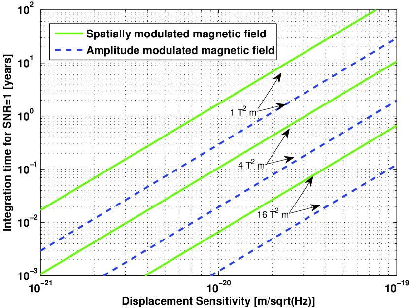
Figure 1: Integration times for a signal-to-noise ratio of unity, as a function of GW detector sensitivity (given as rms values). The lines denote different excitation strengths (as peak-to-peak values) for spatially- and amplitude modulated fields, respectively. Continuous application of a sinusoidal signal is assumed.

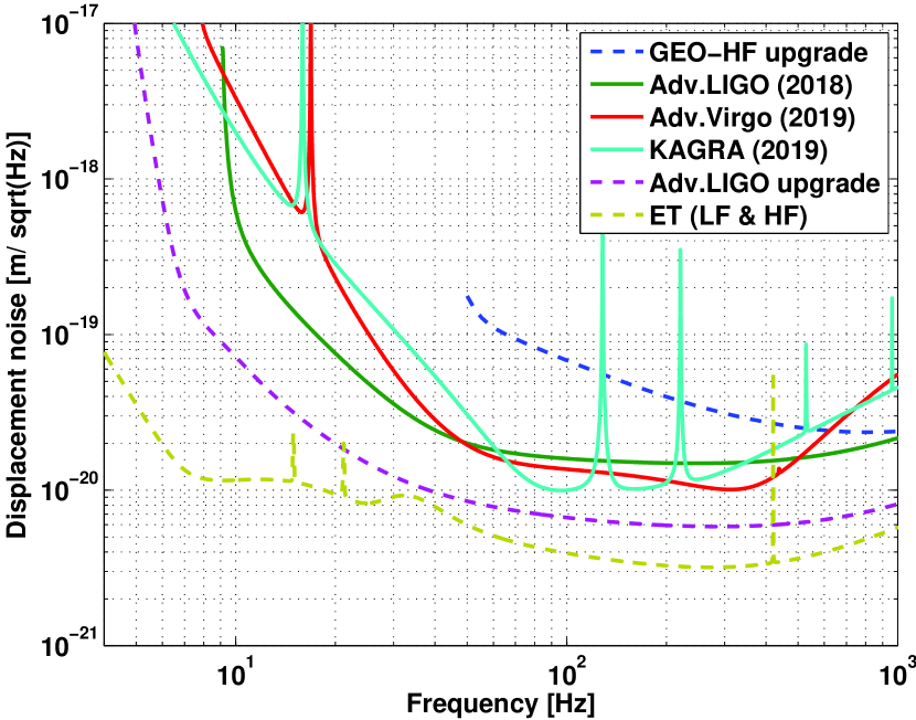
Figure 2: Planned displacement noise curves for laser-interferometric gravitational-wave detectors. Advanced LIGO Harry2010 , Advanced Virgo AdvVirgo2009 , and KAGRA Kagra2012 are under construction, and are denoted with solid lines. The dashed lines denote potential upgrades to GEO-HF GEO-HF and Advanced LIGO, as well as the proposed Einstein telescope ET ET2011 . Years denote estimated/hypothetical times of reaching the target sensitivity. As customary in this field, the noise curves are displayed as root-mean-square amplitude spectral densities.

Figure 1 shows integration times for a SNR of unity, as a function of GW detector sensitivity, according to eq. 7 with continuous application of a sinusoidal signal $S$ being assumed. The graph in Figure 1 shows two lines each, for three different excitation strengths $E$. The solid line assumes the rotation of a static magnetic field around the laser beam axis and thus is suitable to measure $\Delta n_{\parallel-\perp}$. The dashed line assumes an amplitude modulation of the magnetic field, and thus is suitable to measure $\Delta n_{\parallel}$, for a parallel orientation of the magnetic field and the polarization of the light field.

The integration times calculated from eq. 5-7 and shown in Figure 1 are a factor of two longer than the times calculated in reference Zavattini2009 for identical setups. This discrepancy comes from an incorrect assumption on the calibration of GW interferometer strain data Zavattini2013 .

Finally, Figure 2 shows planned displacement sensitivity curves for ground-based laser-interferometric gravitational-wave detectors and potential upgrades. The projects Advanced LIGO Harry2010 , Advanced Virgo AdvVirgo2009 , and KAGRA Kagra2012 are currently under construction and are expected to become operational within the next years. Other projects are potential upgrades Sred2012 or entirely new detectors, as in case of the Einstein Telescope ET ET2011 .

To give an example, for Advanced LIGO and Advanced Virgo we can read a sensitivity of $2\times 10^{-20}\,\rm m/\sqrt{Hz}$ at 50 Hz. With an excitation of $1\,\rm T^{2}m$ for an amplitude-modulated magnetic field (which would have to be modulated at 25 Hz), we get an integration time of a bit more than 1 year for a SNR of unity, according to Figure 1.

While this integration time seems very long, it should be noted that long integration times pose no principal problem here, since the gravitational-wave detectors are expected to run for several years. Obviously, a magnetic field excitation would have to be held active during this time as well. However, such a long integration time would probably be the upper acceptable limit for SNR=1, and either more sensitivity or a stronger field excitation would be desirable in the long run. In the following, we will use the example of a magnet system with $1\,\rm T^{2}m$ for amplitude modulated fields, and the example of $2.3\,\rm T^{2}m$ for rotating fields, which gives similar integration times for the measurement of $\Delta n_{\parallel}$ and $\Delta n_{\parallel-\perp}$, respectively.

III Discussion of possible source field magnets

To illustrate the difficulty of building large strong magnets, it is instructive to calculate the energy stored in a magnetic field, $W=\frac{1}{2\mu_{0}}B^{2}V$, with $\mu_{0}$ being the permeability of the vacuum, and $V$ the volume over which the magnetic field $B$ is erected. If we assume the volume will be of cylindrical shape with radius $r$ around the laser beam axis and extending over a length $D$, we get for the energy $W$:

$$W=\frac{\pi}{2\mu_{0}}B^{2}Dr^{2}$$ (9)

We see that the energy content in the magnetic field increases with the square of the field strength and with the square of the field radius, which is one reason why the design of large and strong magnets is technically challenging.

In order to discuss possible source field magnets which are as small as possible, but as large as necessary for our application, we need to determine the minimum radius $r$ of the usable magnetic aperture through which the laser beam would pass. GW detectors have the laser beams traversing in stainless-steel beam tubes of order 1 m in diameter. However, as has been discussed in Zavattini2009 , possibly a smaller aperture has to be used for vacuum-QED measurements. We propose here to use the smallest aperture possible, as judged by the constraints of the GW detectors’ optical path. Therefore, we note the additional loss that an aperture (due to a section of the beam tube with reduced diameter) would cause. GW detectors use laser beams with a Gaussian beam profile, having a radial intensity distribution of

$$I_{(r)}=I_{0}e^{\frac{-2r^{2}}{w^{2}}}.$$ (10)

Here $I_{0}$ is the intensity at the center of the beam ($r=0$) and $w$ is the (1/e field-) beam radius. From this, the power loss due to clipping of the beam profile is calculated. However, an aperture does not only clip the beam, it also gives rise to diffraction. The laser power diffracted from the central gauss-beam profile is not recovered by the optical resonators within the GW detector and thus lost. The effective loss from diffraction slightly depends on the geometry of the optical resonator within which the aperture is located, such that a simulation FINESSE has been used here, for the example of Advanced LIGO. The results of this simulation correspond to those obtained in Spero when adjusting for the wave-length and cavity geometry used in there.

Figure 3 shows the calculated power loss of a laser beam with Gaussian beam profile as a function of the size of a circular beam clipping aperture. The pure clipping loss is shown separately from the total loss obtained from the simulation.

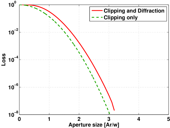
Figure 3: Calculated power loss of a laser beam with Gaussian beam profile with radius $w$, as a function of the size of a circular beam clipping aperture with radius $A_{r}$ (located at the beam waist). Losses due to clipping and total loss (i.e. clipping and diffraction) are shown separately.

Advanced GW detectors are designed to have very low optical losses upon reflection of laser beams on their mirrors. These low losses which should be no more than about 30-50 ppm per reflection are mandatory to allow a high power build-up in the resonant optical cavities. Therefore, and also to minimise scattered light from the aperture, no more than around $1\,ppm$ of extra loss from a reduced tube aperture seems acceptable. Given Figure 3, an aperture radius of 3 beam radii appears as a reasonable choice, yielding about 0.2 ppm (parts per million) loss.

Table 2 shows actual beam sizes of current and planned GW detectors, around the middle of the beam tube, near to the position of the minimum beam size. (GEO 600 is an exception to this, since in the current layout the minimum beam size is located close to the corner-station end of the beam tube.)

GW-IFO	Beam radius at waist [mm]	Minimum aperture (3 x beam radius) [mm]	Realistic aperture radius [mm]
GEO 600	9	27	40
Adv. Virgo	10	30	45
Adv. LIGO	12	36	55
KAGRA	16	48	70
ET-HF	25	75	115
ET-LF	29	87	130

Table 2: Beam radii of existing and planned gravitational-wave detectors, and proposed minimum aperture sizes. In the column ’realistic aperture radius’, 50 % is added to the minimum aperture and the result rounded. This accounts for an additional beam tube and clearance space, as detailed in section IV, however is only an example here, since exact numbers would depend on more details of a chosen setup.

As an example, aiming for an aperture radius of 55 mm and an excitation of $E=1\,\rm T^{2}m$, we calculate the energy stored in the magnetic field of such a magnet to be $W=3781\,\rm J$. For continuously amplitude-modulated fields with a modulation frequency of 25 Hz, this energy has to be brought into and removed from the aperture space 50 times per second, corresponding to an energy flow of almost 200 kJ/sec.

III.1 Electro-magnets

Electro-magnets, modulated in field amplitude, would allow for the measurement of $\Delta n_{\parallel}$ or $\Delta n_{\perp}$. Linear conductors parallel to the laser beam tube are the most efficient way to generate a magnetic field perpendicular to the laser beam direction, a setup also used for beam deflection in particle accelerator magnets. Figure 4 shows a principal setup of a linear magnet arranged alongside a laser beam tube.

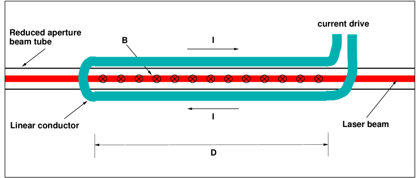
Figure 4: Principal setup of a linear magnet consisting of a conductor loop running mostly in parallel to both sides of a laser beam tube. Some quantities are denoted as used in the text.

We start with the parameter estimation of such a linear conductor, by noting that we want to maximize the excitation $E$, as defined in equation 8 for any magnet design. Eq. 8 is to be resolved to the geometric parameters of the setup, material constants, and electrical power. We use the following equations:

$$B=2\mu_{0}\frac{I}{2\pi r}$$ (11)

with $I$ being the effective current through the linear conductor with distance $r$ from the laser beam axis. This is an approximation assuming a conductor which is long in the laser beam direction, and has a small crossection compared to the dimensions of the beam tube in the plane perpendicular to the beam tube. The factor of two on the left side comes from counting the two conductors at each side of the beam tube. We then use the electrical power dissipation $P$ (in the low frequency limit)

$$P=I^{2}R$$ (12)

with $R$ being the total ohmic resistance of the linear conductor. Finally we use

$$R=\frac{2\rho D}{A}$$ (13)

to calculate the ohmic resistance of the conductor, with $\rho$ being the specific resistance of the conductor material and $A$ being the cross-section of the conductor .

Combining equations (11) to (13) and inserting into (8) we obtain

$$E=\frac{\mu_{0}^{2}}{2\pi^{2}}\frac{PA}{\rho r^{2}}$$ (14)

This result has the following implications for the magnet design:

• The length of the conductor $D$ has been eliminated and hence has no influence on the excitation strength (for a given power, conductor cross-section, and beam tube diameter). Note that this result can be used to adjust the maximal temperature as well as mechanical force on the conductors, as two technical constraints.

• For a fixed tube diameter, the excitation increases with increasing conductor cross-section, up to practical limits not reflected in eq. 14. In principle this can be used for the estimation of a quasi-optimal conductor cross-section.

• Increasing the electrical power $P$ and decreasing the resistance of the conductor material $\rho$ increase the excitation linearly. While copper is the obvious material of choice for the conductor, the power $P$ will be determined by heat dissipation and general power handling constraints of the setup.

• Similar to what was found in eq. 9, the excitation decreases with the square of the distance $r$ to the application region, which thus should be as small as possible.

For a desired excitation of $E=1\,\rm T^{2}m$ and an example conductor cross-section $A\approx r^{2}$ we obtain (using eq. 14) a necessary power of $P\approx 210\,\rm kW$. This is a rather large power and seems very impractical to realize.

A simulation with the finite-element simulator program FEMM FEMM yields $P\approx 300\,\rm kW$, roughly confirming the simplified calculation. Just for illustration, Figure 6 shows the magnetic field lines for this simulation. However, this result is only valid for the low frequency limit, in particular at DC.

While super-conducting magnets can lower the energy dissipation in the conductor due to the extremely low electrical resistance, they are not suitable for large and fast amplitude modulations of the magnetic field, as will be required for our application. Therefore, we only consider copper as conductor material throughout this paper.

For our example, we need to amplitude-modulate the drive current at a frequency $f=25\,\rm Hz$. While the real power dissipation is largely un-affected from this (neglecting skin- and proximity effects), the inductance of the setup results in very large reactive powers to be handled. The numerical calculation with FEMM yields a reactive power of $P=2.5\,\rm MW$, which very much complicates the electric drive circuit on top of the real power dissipation of the system as calculated above.

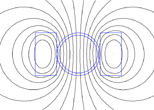
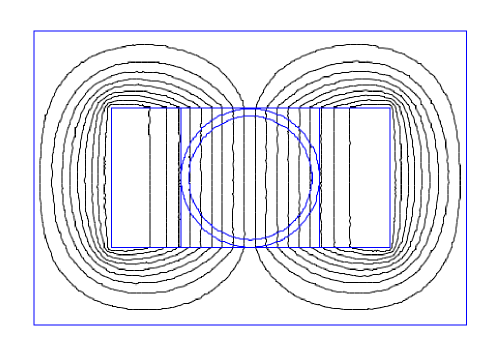
Figure 5: Setup and simulated magnetic field lines for a linear conductor of rectangular shape to both sides of the central circular vacuum tube. This is the cross-sectional view of the setup as in Figure 4.

Figure 6: Setup and simulated magnetic field lines for the same setup as in Figure 6, but with the addition of ferro-magnetic material around the rectangular conductors and the central vacuum tube.

Field enhancement with ferro-magnetic material

If the peak magnetic fields are constrained to about 2 T, it can be considered to use a ferro-magnetic material to enhance the magnetic flux for a given magnetic setup. This has been simulated for the example above, adding a soft ferro-magnetic material (US-steel type S-2, with 0.018 inch lamination) in the FEMM simulation around the copper conductor, as depicted in Figure 6. The electrical drive power has been adjusted to again yield an excitation of $E=1\,\rm T^{2}m$. The simulation result is that in the low frequency limit the power is reduced to $P=45\,\rm kW$. If modulated at a frequency of $f=25\,\rm Hz$ the reactive power is now $P=1\,\rm MW$. This is better, but still seems far from practical to realize.

III.2 Pulsed electro-magnets

As will be shown in the following, continuous operation of an electro-magnet (at a fixed frequency) is not optimal. For the same average power $P$ applied to the magnet, the total integration time for a given SNR can be reduced if the magnet is active only for fractions of time, intersperced by pauses.

If equation 7 is combined with equation 14, we obtain

$$t_{SNR=1}\sim\left(\frac{\tilde{n}(f)}{P}\right)^{2}$$ (15)

We define $P=P_{p}\times\eta_{p}$ with $P_{p}$ being the power applied to the magnet during a fraction $\eta_{p}$ of the time, such that the average power $P$ is kept constant. After a few steps we then get

$$t_{SNR=1}\sim\eta_{p}\times\left(\frac{\tilde{n}(f)}{P}\right)^{2}$$ (16)

Notably, this is the same result as in equation 15, except for the factor $\eta_{p}$, which implicitly is $\eta_{p}=1$ for the case of continuous operation of the magnet. We see that the integration time is linearly reduced with the fraction of time that the magnet is engaged (keeping the average power $P$ constant). This is the basic motivation to use a pulsed operation of electro-magnets in the first place. Ultimately this technique is limited by the peak power and pulse energy that can be handled by the system, which is determined by the pressure on the conductors due to Lorentz forces and by constraints in the electrical drive system. Another limit on $\eta_{p}$ comes from the usable signal period $T=1/f$, which preferably has to match the frequency of lowest noise of the GW detector, as relevant for our application. However besides these more technical constraints, we also have neglected so far the energy $W_{m}$ needed to build up the magnetic field. To include this energy into the calculation we split the total energy $W_{p}$ of a single pulse into the components due to electrical dissipation in the conductor $W_{E}$ and the energy in the magnetic field $W_{m}$. For $W_{P}=W_{E}+W_{M}$ we obtain:

$$W_{P}=\frac{L}{2}I^{2}+t_{P}RI^{2}$$ (17)

with $L$ being the inductance of the conductor setup, and $t_{P}$ being the length of the pulse. For a linear conductor setup according to Figure 4 the inductance L can be approximated as $L=D\mu_{0}/\pi$. Resolving equation 17 to the current $I$, inserting into equations  11 and then into  8, we obtain (with also using equation 13):

$$E=\frac{\mu_{0}^{2}}{\pi^{2}r^{2}}\frac{W_{P}}{\frac{\mu_{0}}{2\pi}+\frac{2\rho}{A}t_{P}}$$ (18)

This result is equal to equation 14, if the constant term $\frac{\mu_{0}}{2\pi}$, which resembles the energy stored in the magnetic field, is neglected. The implications are:

• If the cross-section $A$ of the conductor is small, the energy dissipation $W_{E}$ will dominate over the energy $W_{M}$ in the magnetic field. This is a typical operation regime for most pulsed magnets.

• If the pulse duration $t_{P}$ gets too short, $W_{M}$ will dominate over $W_{E}$ such that the excitation $E$ is not increasing any more for shorter pulses.

• Obviously the excitation $E$ scales with the total pulse energy $W_{P}$, and inversely with the square of the system size $r$.

A single pulse of length $t_{P}$ with energy $W_{P}$ results in a power $P_{P}=W_{P}/t_{P}$. To keep the average power $P$ at a fixed lower level we apply pulses only every $t_{p}/\eta_{p}$ seconds, again with $\eta_{p}=P/P_{P}$. In order to calculate integration times according to equation 7, we then have to use

$$t_{SNR=1,pulsed}=\frac{t_{SNR=1}}{\eta_{p}}$$ (19)

For a pulse energy of 1 MJ, an aperture radius of $r=55\,\rm mm$, a conductor cross-section of $A\approx r^{2}$, and an average power of $P=20\,\rm kW$ we calculate integration times for SNR=1 as shown in Figure 7. A GW detector sensitivity of $\tilde{n}(f)=2\times 10^{-20}\,\rm m/\sqrt{Hz}$ is used for all frequencies, in order to illustrate the effect of the energy in the magnetic field on the optimal pulse length .

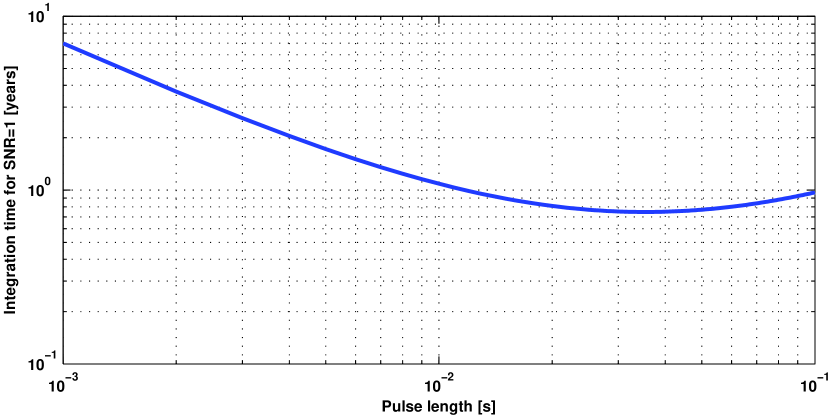
Figure 7: Integration times as function of pulse length. The parameters used are a pulse energy of $W_{P}=1\,\rm MJ$, aperture radius $r=55\,\rm mm$, and a conductor cross-section of $A\approx r^{2}$. A GW detector sensitivity of $\tilde{n}(f)=2\times 10^{-20}\,\rm m/\sqrt{Hz}$ is used for all frequencies

For a pulse length of $t_{p}=10\,\rm ms$ we get an integration time around 1 year, which means that about 600000 pulses would have to be applied. While the average power has been lowered compared to the examples above, a pulse energy of 1 MJ is on the edge of current technology and is a very optimistic assumption given that the magnet for this application would still need to be developed. An energy of 1 MJ corresponds to 240 g of the explosive TNT.

Further, for the estimations in this section we have made simplifying assumptions, particularly not taking into account the following parameters: forces between the conductors and within the conductors, temperature rise of the conductor, skin effect, proximity effect, and complexities of the power supply. All these factors contribute to the complexity of (pulsed) magnet design, and typically make achieving the calculated performance demanding in practice.

The use of pulsed magnets for vacuum-QED measurements at GW detectors was proposed and evaluated in ref. Doebrich2009 . The estimation of integration times is more accurate in there, since the authors look at the full frequency spectrum of a signal pulse whereas we made simplifying assumptions in the estimation above. However, the authors in Doebrich2009 concentrated on the principal ideas of the approach, and did not consider a possibly realistic experimental setup. One very optimistic assumption in their work is the estimation of an aperture diameter (through which the laser beam passes) of the magnetic field of order cm, which is the aperture available from pairs of pulsed Helmholtz coils under development in the Dresden high-field laboratory Doebrich2009 . However, as shown above, a realistic assumption is a necessary aperture diameter of order 10 cm. This difference is the main single reason why the conclusion about the feasibility of using pulsed magnets for QED measurements at GW detectors is much more pessimistic in the estimation described in this section.

III.3 Permanent magnets

The development of permanent magnet materials has made significant progress over the last decades, with the current maximum of a typical remanent magnetic flux density around $B_{r}=1.3\,\rm T$ for neodymium-iron-boron ($Nd_{2}Fe_{14}B$) magnets. With superposition arrangements of individual magnet domains it is possible to obtain even larger magnetic field strengths, as for example with a Halbach array Halbach1980 . If arranged in a Halbach cylinder configuration, a uniform magnetic field within a hollow cylinder can be obtained, with its field lines oriented perpendicular to the cylinder axis. The new design of the PVLAS experiment uses such Halbach cylinders for the ellipsometric vacuum-QED measurement attempt Valle2013 .

Figure 8 shows a Halbach cylinder of length $D$ with an outer radius $r_{o}$ and a central opening of radius $r_{i}$. The magnetic domain orientations are depicted on the left front face of the cylinder. The laser beam passes through the central opening, and the cylinder would be rotated around the laser beam axis, to provide spatial modulation of the magnetic field.

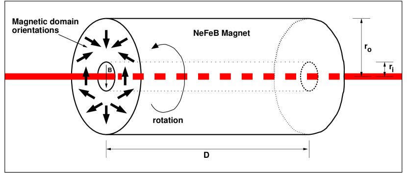
Figure 8: Illustration of a Halbach cylinder with central opening, magnetized to yield a uniform magnetic field perpendicular to a laser beam passing the cylinder.

The magnetic field strength $B$ of a cylinder according to Figure 8 can be approximated by

$$B=B_{r}\times ln\frac{r_{o}}{r_{i}}$$ (20)

with $B_{r}$ being the remanent field strength of the magnet material. Such a magnet can be used to spatially modulate the magnetic field by rotation of the field around the laser beam, and thus measure $\Delta n_{\parallel-\perp}$. A magnet with excitation $E=2.3\,\rm T^{2}m$ could be constructed by choosing $B_{r}=1.3\,\rm T$, $r_{o}/r_{i}=2.2$, and $D=2.25\,\rm m$. Similar magnets have already been fabricated for the new PVLAS experiment Valle2013 , although with a smaller inner radius $r_{i}$ than for this application, where we are aiming for $r_{i}=55\,\rm mm$. Another similar magnet, for an aperture radius of 13.5 mm, has been designed for the Q&A experiment. This design is similar to a Halbach cylinder, but also includes soft magnetic materials to increase the flux density towards the application region Wang2004 . However, given the total mass of the assembly, there seems to be no significant advantage over the standard Halbach cylinder design.

An obvious large advantage of permanent- over electro-magnets is the fact that once the magnet has been constructed, there is no shifting of energy in- and out of the magnetic field required, and also no electrical power is dissipated in order to generate the field. With the magnet described here, rotating at $f=25\,\rm Hz$ around a GW detector laser beam with a displacement noise of $\tilde{n}(\rm 50Hz)=2\times 10^{-20}\,\rm m/\sqrt{Hz}$, the integration time for n SNR=1 would again be about 1 year.

Nested Halbach cylinders

The disadvantage over electro-magnets is that in the setup using a single Halbach cylinder, only $\Delta n_{\parallel-\perp}$ can be measured. However, this could be overcome by using two Halbach cylinders nested into each other. With such an arrangement it would be possible to amplitude-modulate the magnetic field inside the inner cylinder, simply by superposition of the fields of the two cylinders. The orientation of the magnetic field lines stays constant and thus $\Delta n_{\parallel}$ or $\Delta n_{\perp}$ can be measured individually. The relative forces between the two cylinders are small in the ideal case, where the outer fields are close to zero. Whether this approach would be feasible in practice would need further investigation, and also depends on the rotation speed of the magnets.

IV A scenario to measure vacuum-QED effects with GW detectors

Figure 9 shows a possible principal layout of a vacuum-QED measurement at the beam line of a gravitational wave detector. A section of the main beam tube is replaced with a non-conducting section with small aperture. This tube should be electrically non-conducting to avoid attenuation of the usable magnetic field by eddy-currents . Eddy currents would also heat the tube, and could lead to undesired mechanical forces.

Seismically isolated baffles are proposed to prevent any light hitting the reduced beam tube, where scattering of laser light could produce excess noise in the GW detector readout Takahashi2004 . The baffles should have a central opening that is slightly smaller (e.g. by a few mm) than that of the reduced beam tube, such that no light will hit the beam tube in the interaction region with the magnetic field. Obviously, the baffle opening diameter is then the limiting aperture for the laser beam losses, and the amount by which this aperture is smaller than the beam tube diameter determines how well the alignment of baffle and beam tube has to be set and maintained against each other.

The Cotton-Mouton effect (CME) Cotton1905 of residual gas should be sufficiently low if the total pressure is held at less than $0.5\,\rm\mu Pa$, as far as the main constituents of air are concerned. With estimated CMEs for molecular nitrogen and oxygen of $\Delta n_{\parallel-\perp}(N_{2})\approx 2\times 10^{-12}/(10^{5}\,\rm Pa\,T^{2})$ and $\Delta n_{\parallel-\perp}(O_{2})\approx 2\times 10^{-13}/(10^{5}\,\rm Pa\,T^{2})$ as taken from Rizzo1997 , we approximate the CME for air ($78\,\rm\%N_{2}$ and $21\,\rm\%O_{2}$) as $\Delta n_{\parallel-\perp}(air)\approx 6\times 10^{-13}/(10^{5}\,\rm Pa\,T^{2})$. With a total pressure of $0.5\,\rm\mu Pa$ we obtain a contribution from residual air of $\Delta n_{\parallel-\perp}(air)\approx 3\times 10^{-24}/\rm T^{2}$, just below the expected QED effect as given in equation 3.

The CME for water in the gas phase has been measured in Valle2014 to $\Delta n_{\parallel-\perp}(H_{2}O)\approx 6.7\times 10^{-15}/(10^{5}\,\rm Pa\,T^{2})$, yielding a partial pressure of $\approx 60\,\rm\mu Pa$ to be equal to the expected QED effect.

If a residual gas analyzer is used for permanent monitoring of the partial pressures, and the CMEs of the residual gases are known sufficiently well, the estimated CME contributions can be subtracted from the vacuum QED signal thus increasing the significance with which a vacuum QED effect can be isolated.

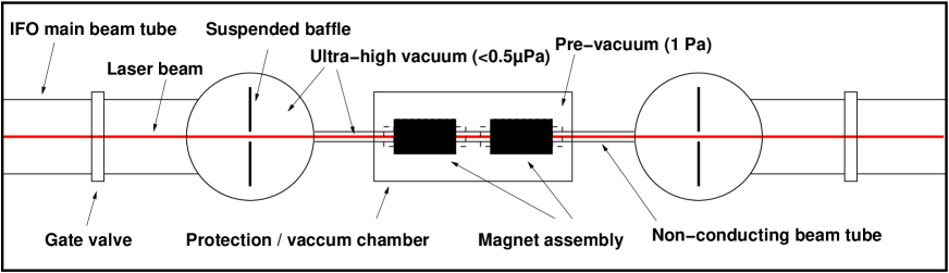
Figure 9: Possible principle layout of a vacuum-QED measurement at the beam line of a gravitational-wave detector. A section of the main beam tube is replaced with a non-conducting section with small aperture. Seismically isolated (suspended) baffles prevent light from being scattered at the interaction beam line. Spatially or temporal modulated magnetic fields are generated by magnets located around the interaction beam line. In case these magnets are solenoid magnets to be rotated with high speed, additional pre-vacuum chambers might be required, as depicted in the figure.

The main constructional challenge would be the assembly and precise alignment of the reduced beam line setup and the suspended baffles. Once this is done without degradation of the GW detector sensitivity, the magnet experimental setup should not interfere with the GW detector operations. As discussed above, the best option seems to be permanent magnets rotating around the beam axis. As planned for the new PVLAS experiment, it is a good idea to use at least two magnets. This opens the possibility to make null-measurements, when the magnetic fields of the two magnets are kept perpendicular to each other during rotation, thus testing for systematic errors due to false signals. While more unlikely in a GW detector, such signals have been observed in the ellipsometric experiments as described in section I. In GW detectors the interaction region with the magnetic field would typically be at the middle of the beam tube, thus of order $\sim\rm km$ away from the end stations holding the test-masses, which minimizes the risk of direct interaction of the magnetic field with the test masses or other components of the detection system.

Of course it is possible in principle that more systematic errors would be discovered during the experiment. Systematic errors are commonly the biggest unknown in high-precision experiments, and have been slowing down the progress (not only) of other vacuum-QED projects. For example, vibrations of the beam tube at twice the magnet rotation frequency might be caused by (inhomogeneous) residual ferro-magnetic contamination or diamagnetism / paramgnetism of the beam tube material . These vibrations could couple to the laser beam (and thus may cause a spurious signal) in principle, for example if the shielding of the gaussian tail of the laser beam by the baffles would not be sufficient. However, it would be possible to measure the vibration of the beam tube, and for an additional null-test, one could excite a similar beam tube motion as under magnet rotation, but without actually rotating the magnets. Another possibility to exclude such an effect would be to compare (QED-) measurements under different conditions of mechanical damping of the beam tube.

In order to estimate a limit for the vibration of the baffles at the signal frequency one has to make an assumption on the scatter of light from the baffle into the main beam of the interferometer and compare its contribution to a putative QED signal. A very conservative estimate would be that a fraction $P_{S}=10^{-10}$ of the main beam power would be scattered into the fundamental Gaussian mode , corresponding to a fraction $A_{S}=\sqrt{P_{S}}=10^{-5}$ of the scattered light field amplitude. (Note that less than 1 ppm of power should be lost due to forward scattering and clipping at the baffle, as discussed in section III. Only a very small fraction of the clipped light can be scattered back into the fundamental laser mode in principle.) An excitation of $1\,\rm T^{2}m$ makes a signal of about $S\approx 10^{-24}\,\rm m$ (eq. 3 - 6) at frequency $f$, corresponding to a phase shift of $2\pi/\lambda\times S\approx 6\times 10^{-18}\,\rm radian$ (with $\lambda=1064\,\rm nm$ being the wave-length of the light). Therefore, the baffle motion at frequency $f$ should be less than $S/A_{S}\approx 10^{-19}\,\rm m$. For a (hypothetical) motion of the baffle suspension point of order $10^{-12}\,\rm m$ at frequency $f$, one would thus need 7 orders of magnitude of isolation from the baffle suspension. If we take $f=50\,\rm Hz$ as signal frequency, this is achievable with three stages of isolation (for example one passive stack/rubber pre-isolation and a double pendulum suspension for the baffle.) It is hard to predict what vibration level one may get at the suspension point. However, this level can be measured precisely with accelerometers, and the baffle suspension point could also be artificially excited to estimate the amount of signal contribution from scattering at the baffle.

Regarding the magnet design, a calculation of excitation per unit of material cost shows that a ratio of $r_{o}/r_{i}=2.2$ is close to the optimum, as shown in Figure 10.

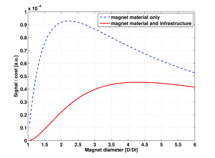
Figure 10: Excitation per unit of cost as function of the radius ratio $r_{o}/r_{i}$ for a Halbach cylinder as depicted in Figure 8. The maximum efficiency is around a ratio of 2.2 when only magnetic material and bearing cost are accounted for. Additional cost of infrastructure that grows linear with length of beam tube occupied by the setup can lead to an optimal ratio of 3.5-5.

For the bearing and rotational drive of the magnets, it seems best to use friction-less magnetic bearings Schweitzer2002 , which would be particularly helpful for the long integration times needed. The cost of such bearings roughly scales with the mass they can support, such that the cost optimization including bearings is the same as for magnet material only, as shown in Figure 10. As an example, one could use two magnets with excitation $E=1.2\,\rm T^{2}m$, and length $D=1.2\,\rm m$ each. For a ratio $r_{o}/r_{i}=2.2$, and an inner radius of $r_{i}=55\,\rm mm$, the mass of one magnet would be 328 kg and it would cost around $ 50000 at current material prices. For the two magnets, the integration time for a SNR=1 would be t=1.07 years. The situation gets better if the sensitivity of the GW detectors is improved in the future. For example, a displacement noise of $8.5\times 10^{-21}\,\rm m/\sqrt{Hz}$ at 50 Hz might be reached by a potential upgrade of Advanced LIGO (see Figure 2). Together with increasing the number of magnets from 2 to 4, the integration time for SNR=1 would fall to t=17.7 days, such that after 3 years of operation a reasonably good SNR of 8 could be achieved for the basic QED effect.

V Conclusion

Laser-interferometric gravitational wave detectors currently under construction or planned for the future offer the possibility of vacuum-QED measurements. We have shown the principal feasibility of this approach given the planned sensitivities and magnet technology, and derived new estimates of measurement times. We have compared three different kinds of source field magnets and conclude that from a realistic design perspective, permanent magnets are the best, or even the only, option for the time being. The main implementation work will come from the reduction of beam tube diameter, given the constraint to not disturb the gravitational-wave measurement capability of the instrument. Even if vacuum-QED measurements would be successful by ellipsometric measurements within the next several years, the measurement of these effects with GW detectors is still valuable since it is based on a different measured quantity, the velocity shift of the light, and also has the potential to measure parameters of exotic particle models not accessible with ellipsometric measurements.

References

- (1) W. Heisenberg and H. Euler, Z. Phys. 98 (1936) 714
- (2) B. Döbrich, H. Gies, Europhysics Letters 87, 21002 (2009).
- (3) F. Della Valle, et.al., Optics Communications 283, 4194-4198 (2010).
- (4) F. Della Valle, U. Gastaldi, G. Messineo, E. Milotti, R. Pengo, L. Piemontese, G. Ruoso, G. Zavattini, New J. Phys. 15, 053026 (2013)
- (5) F. Della Valle, E. Milotti, A. Ejlli, G. Messineo, L. Piemontese, G. Zavattini, U. Gastaldi, R. Pengo, and G. Ruoso, Physical Review D, accepted for publication (2014), preprint: arXiv 1406.6518
- (6) R. Battesti, et.al., Eur. Phys. J. D 46, 323-333 (2008)
- (7) P. Berceau, M. Fouche, R. Battesti, C. Rizzo, Physical Review A 85, 013837 (2012)
- (8) A. Cadène, P. Berceau, M. Fouché, R. Battesti, C. Rizzo Euro Phys. J. D, 68:16 (2014)
- (9) S.J. Chen, H.H. Mei, and W.T. Ni, Mod. Phys. Lett. A, 22 (2007) 281.
- (10) Pugnat et al., CERN-SPSC-2006-035, see http:// graybook.cern.ch/ programmes/ experiments/ OSQAR.html
- (11) T. Heinzl, B. Liesfeld, K.U. Amthor, H. Schwoerer, R. Sauerbrey, and A. Wipf, Opt. Commun., 267 (2006) 318
- (12) F. Bielsa, A. Dupays, M. Fouché, R. Battesti, C. Robilliard and C. Rizzo, Appl. Phys. B 97, 457-463 (2009)
- (13) D. Boer, J.W. van Holpen, arXiv arXiv:hep-ph/0204207v1 (2002)
- (14) R. Battesti and C. Rizzo, Rep. Prog. Phys. 76, 016401 (2013)
- (15) A.M. Grassi Strini, G. Strini, and G. Tagliaferri, Physical Review D 19 No 8, 2330-2335 (1979)
- (16) V.I. Denisov, I.V. Krivchenkov, N.V. Kravtsov Physical Review D 69 066008 (2004)
- (17) G. Zavattini, E. Calloni, Eur. Phys. J. C 62, 459-466 (2009)
- (18) S. Askenazy, C. Rizzo, O. Portugall, Physica B 294-295, p. 5-9 (2001).
- (19) S. Batut, et.al., IEEE TRANSACTIONS ON APLLIED SUPERCONDUCTIVITY 18 No 2, 600-603 (2008).
- (20) G. M. Harry and the LIGO Scientific Collaboration Classical and Quantum Gravity 27 No 8, 084006 (2010)
- (21) The Virgo Collaboration note VIR–027A–09 https://tds.ego-gw.it/itf/tds/file.php?callFile=VIR-0027A-09.pdf (2009)
- (22) K. Somya, Classical and Quantum Gravity 29 No 12, 124007 (2012)
- (23) H. Lück et. al. J. Phys.: Conf. Ser. 228, 012012 (2010)
- (24) S. Hild, https://dcc.ligo.org/LIGO-T1200046 (2012)
- (25) S. Hild et. al., Classical and Quantum Gravity 28, 094013 (2011)
- (26) K. Halbach, Nuclear Instruments and Methods 169, 1-10 (1980)
- (27) G. Zavattini, personal communication
- (28) A. Freise et. al., http://www.gwoptics.org/finesse/
- (29) R. E. Spero, https://dcc.ligo.org/T920002/public (1992)
- (30) D. C. Meeker, Finite Element Method Magnetics, http://www.femm.info
- (31) Z. Wang, W. Yang, T. Song, and L. Xiao, IEEE Transactions of Applied Superconductivity 14 No.2 (2004)
- (32) R. Takahashi, K. Arai, S. Kawamura, and M. R. Smith Phys. Rev. D 70 062003 (2004)
- (33) A. Cotton and H. Mouton, Ct.r.hebd. Seanc Acad. Sci., Paris 141, 317,349 (1905)
- (34) C. Rizzo, A. Rizzo, and D. M. Bishop, Int. Rev. Phys. Chem 16:1 81-111 (1997)
- (35) F. Della Valle, A. Ejlli, U. Gastaldi, G. Messineo, E. Milotti, R. Pengo, L. Piemontese, G. Ruoso, G. Zavattini Chem. Phys. Letters 592 288-291 (2014)
- (36) G. Schweitzer Proc. 6th Internat. IFToMM Conf. on Rotor Dynamics, Sydney, Sept. 30-Oct. 3 (2002)