On Parton Number Fluctuations

Abstract

Parton evolution with the rapidity essentially is a branching diffusion process. We describe the fluctuations of the density of partons which affect the properties of QCD scattering amplitudes at moderately high energies. We arrive at different functional forms of the latter in the case of dipole-nucleus and dipole-dipole scattering.

1 Quantum chromodynamics at high density

Quantum chromodynamics in the high-energy/high-density regime is a very rich field from a theoretical viewpoint since it involves genuinely nonlinear physics, and nontrivial fluctuations. The latter are deemed a goldmine for modern physics [1]. From a phenomenological viewpoint, there is a wealth of data from different experiments which await interpretation. (For a review, we refer the reader to the recent textbook by Kovchegov and Levin [2]).

Electron-proton (or better, nucleus) scattering is maybe the best experiment to probe QCD in this regime, as was done at HERA, an $e^{\pm}p$ facility. The electron interacts with the proton through a quark-antiquark pair, which appears as a quantum fluctuation of a (virtual) photon of the Weizsäcker-Williams field of the electron. The probability amplitudes for these fluctuations follow from a simple QED calculation. The $q\bar{q}$ pair is a color dipole, and hence electron-hadron scattering may be related to dipole-hadron scattering. If one looks at events in which the $q\bar{q}$ pair has a small-enough size (as compared to the typical size of a hadron), as is possible by selecting longitudinally-polarized highly-virtual photons, then perturbative QCD may be used as a starting point to compute some properties of the dipole-hadron scattering amplitudes.

As for the interaction of protons and/or nuclei as is currently performed at the LHC, the observables need to be carefully chosen if one wants to be able to predict cross sections from first principles – at least in the present state of the art of the theory. Indeed, one needs a hard momentum scale to justify the use of perturbation theory, and the latter must be found in the final state in the form of e.g. the transverse momentum of a jet. It turns out that an observable such as $p_{\perp}$-broadening in proton-nucleus collisions, namely the transverse momentum distribution of single jets, may also be related to the dipole-nucleus amplitude.

We will first review the formulation of the rapidity evolution of the dipole-nucleus scattering amplitude in QCD in the high-energy limit. The latter is given by the Balitsky-Kovchegov (BK) equation. We will relate the known shape of its solution to gluon-number fluctuations in the quantum evolution of the dipole. We will then be able to predict the form of geometric scaling for dipole-dipole scattering, which turns out to be different from the solution to the BK equation.

2 Dipole-nucleus scattering

Let us start with the scattering of a dipole off a nucleus at relatively low energy. The forward elastic amplitude $T$ is a function of the dipole size $r_{0}$, which is given by the McLerran-Venugopalan model:

$$T(r_{0})=1-e^{-\frac{r_{0}^{2}Q_{A}^{2}}{4}}.$$ (1)

This formula resums multiple exchanges of pairs of gluons between the bare dipole and the nucleus (see Fig. 1a). $Q_{A}$ is the saturation momentum of the nucleus. Equation (1) essentially means that a dipole of size larger than $\sim 1/Q_{A}$ is absorbed ($T\sim 1$), while the nucleus is transparent to dipoles of size smaller than $\sim 1/Q_{A}$. For our purpose, we may approximate $T(r_{0})$ by the step function $\Theta(\ln r_{0}^{2}Q_{A}^{2}/4)$.

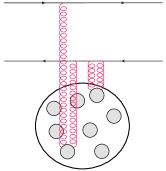
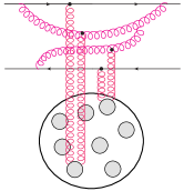
		$\underset{\begin{minipage}[c]{34.14322pt}{\footnotesize large $N_{c}$}\end{minipage}}{\huge\simeq}$
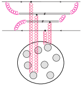
(a)		(b)

Figure 1: Particular graphs contributing to the dipole-nucleus scattering amplitude at low (a) and high (b) energy in the restframe of the nucleus.

Going to higher energies $\sqrt{s}$ by increasing the rapidity of the dipole, the scattering process gets dominated by high-occupancy quantum fluctuations of the initial dipole (see Fig. 1b). The rapidity ($y\equiv\ln s$) dependence of the amplitude is given by the Balitsky-Kovchegov (BK) equation

$$\partial_{y}T(r_{0},y)=\bar{\alpha}\int\frac{d^{2}r_{1}}{2\pi}\frac{r_{0}^{2}}{r_{1}^{2}(r_{0}-r_{1})^{2}}\left[T(r_{1},y)+T(r_{0}-r_{1},y)-T(r_{0},y)-T(r_{1},y)T(r_{0}-r_{1},y)\right]$$ (2)

($\bar{\alpha}\equiv\frac{\alpha_{s}N_{c}}{\pi}$), whose large-$y$ solutions are traveling waves, namely fronts which translate (almost) unchanged in shape towards negative values of the $\ln r_{0}^{2}$ variable as the rapidity increases. The linear part of this equation (the first three terms in the r.h.s.) form the BFKL equation, whose kernel possesses as eigenfunctions the power functions $|r_{0}|^{2\gamma}$, the corresponding eigenvalues being $\bar{\alpha}\chi(\gamma)$, where $\chi(\gamma)\equiv 2\psi(1)-\psi(\gamma)-\psi(1-\gamma)$. Introducing the particular eigenvalue $\chi(\gamma_{0})$, where $\gamma_{0}$ is such that $\chi^{\prime}(\gamma_{0})=\chi(\gamma_{0})/\gamma_{0}$, the shape of $T$ as a function of the dipole size $r_{0}$ in the region $T\ll 1$ and the $y$-dependence of the saturation scale read

$$T(r_{0},y)\underset{r_{0}\ll 1/Q_{s}(y)}{\sim}\ln\frac{1}{r_{0}^{2}Q_{s}^{2}(y)}e^{\gamma_{0}\ln({r_{0}^{2}Q_{s}^{2}(y)})}\ \ \text{and}\ \ Q_{s}^{2}(y)/Q_{A}^{2}\simeq e^{\bar{\alpha}\chi^{\prime}(\gamma_{0})y}.$$ (3)

The BK equation (2) can be established in the framework of the dipole model (see e.g. [2]), where gluons are replaced by zero-size $q\bar{q}$ pairs. In this model, the Fock state of the incoming dipole which is “seen” by the nucleus at the time of the interaction is built from successive independent splittings of dipoles. At a given rapidity $y$, the latter Fock state can be thought of as a collection of $n$ dipoles, generated by a splitting process which belongs to a class of processes generically called branching diffusion.

The main point we wanted to make at this conference and in Ref. [3] was that $T$ has an elegant and useful probabilistic interpretation in the dipole picture: It represents the probability that the largest dipole present in the Fock state of the incoming $q\bar{q}$ pair at the time of the interaction has a size which is larger than the inverse nuclear saturation momentum, $1/Q_{A}$. Indeed, according to the McLerran-Venugopalan model, a given dipole interacts with the nucleus only if its size is larger than $1/Q_{A}$, hence it is necessary and sufficient that at least one of the dipoles in the Fock state be larger than $1/Q_{A}$ for the scattering to take place. Thus solving the BK equation amounts to understanding the statistics of the extremal particles in a branching random walk (BRW). Our first task is to recover the shape of the amplitude (3), previously obtained through a analysis of the BK equation, from the latter statistics.

We observe that the extremal particle in a BRW has fluctuations which can originate only from two places: From the first stages of the rapidity evolution, when the overall number of dipoles is small and thus subject to large statistical fluctuations (we shall call this type of stochasticity “front fluctuations”), and from the tip of the distribution, where by definition, particle numbers keep small. Elsewhere, the evolution is essentially deterministic since it acts on a large number of objects.

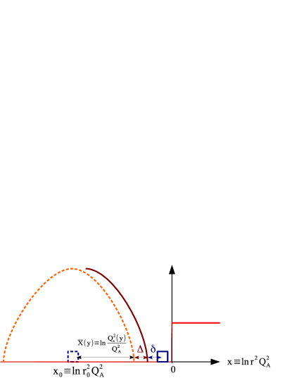
(a)	(b)

Figure 2: (a) Sketch of the dipole distribution (as seen at a given impact parameter) in a particular realization of the evolution to the rapidity $y$ of an initial dipole of size $r_{0}$. (b) Model for the evolution of a given realization, with the “front” and “tip” fluctuations described in the text.

The effect of the front fluctuations is to shift the particle distribution by $\Delta$. We conjecture that the distribution of $\Delta$ is $\propto e^{-\gamma_{0}\Delta}$. The effect of the tip fluctuations is instead to send randomly particles ahead of the front by $\delta$. We conjecture the same exponential law $\propto e^{-\gamma_{0}\delta}$.

We introduce our notations in Fig. 2. According to the previous discussion, in a particular event, the scattering occurs if $x_{0}+\bar{X}(y)+\Delta+\delta\geq 0$. Hence the amplitude $T$ simply is the average of this condition over $\Delta$ and $\delta$:

$$T\propto\int_{0}^{+\infty}d\delta\,e^{-\gamma_{0}\delta}\int_{0}^{+\infty}d\Delta\,e^{-\gamma_{0}\Delta}\Theta(x_{0}+\bar{X}(y)+\Delta+\delta)\propto(-x_{0}-\bar{X}(y))e^{\gamma_{0}(x_{0}+\bar{X}(y))}.$$ (4)

Switching back to the QCD variables, we recover the expression of $T$ given in Eq. (3). We conclude that the shape of the dipole-nucleus scattering amplitude as a function of the dipole size is directly related to the event-by-event fluctuations of the size of the largest dipole, which in turn stem from the fluctuations of the numbers of gluons produced in the QCD evolution.

3 Dipole-dipole scattering

While the dipole-nucleus amplitude probes the statistics of the largest dipole in the quantum evolution, the physics of dipole-dipole scattering is a bit different: Indeed, since the elementary amplitude (for dipoles of respective sizes $r_{0}$ and $R_{0}$) at zero rapidity is essentially $T(r_{0},R_{0})\sim\alpha_{s}^{2}\delta(\ln r_{0}^{2}/R_{0}^{2})$, it is the very shape of the dipole number distribution that is actually probed (Fig. 3). So in order to compute the shape of the amplitude, we need on one hand the probability distribution of the front fluctuations used before, and on the other hand the shape of the dipole number density from the deterministic evolution. We also need to implement saturation in the evolution (see Fig. 3c) to comply with the unitarity constraint $T\leq 1$. All in all, we obtain

$$T(r_{0},y)\underset{r_{0}\ll 1/Q_{s}(y)}{\sim}\ln^{2}\frac{1}{r_{0}^{2}Q_{s}^{2}(y)}e^{\gamma_{0}\ln({r_{0}^{2}Q_{s}^{2}(y)})}\ \ \text{where}\ \ Q_{s}^{2}(y)R_{0}^{2}\simeq e^{\bar{\alpha}\chi^{\prime}(\gamma_{0})y}.$$ (5)

Interestingly enough, it differs from the dipole-nucleus case; compare Eq. (3) to Eq. (5). This is the main prediction of the way of looking at QCD evolution we have promoted at this conference and in Ref. [3].

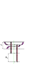
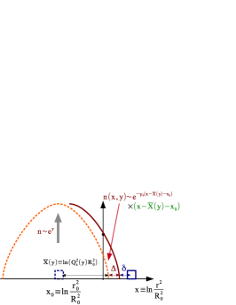
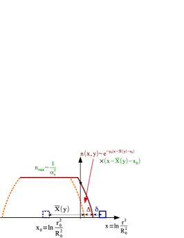
(a)	(b)	(c)

Figure 3: (a) Graph contributing to dipole-dipole scattering at high energies. (b) Sketch of the evolution of the dipole number density, model including fluctuations. (c) The same, but with saturation.

We refer the reader to [3] for the details, references, and more results, in particular on the finite-$y$ corrections to the saturation scale in both the dipole-dipole and dipole-nucleus cases.

References

- [1] E. Scapparone, plenary talk at this conference.
- [2] Y.V. Kovchegov and E. Levin. Quantum Chromodynamics at High Energy. Cambridge Monographs on Particle Physics, Nuclear Physics and Cosmology. Cambridge University Press, 2012.
- [3] A. H. Mueller and S. Munier, Phys. Lett. B 737 (2014) 303.
- [4] A. H. Mueller and S. Munier, “Phenomenological picture of fluctuations in branching random walks,” arXiv:1404.5500 [cond-mat.dis-nn] to appear in Phys. Rev. E (2014).