Hyperfine excitation of N₂H⁺ by H₂: Toward a revision of N₂H⁺ abundance in cold molecular clouds

Abstract

The modelling of emission spectra of molecules seen in interstellar clouds requires the knowledge of collisional rate coefficients. Among the commonly observed species, N₂H⁺ is of particular interest since it was shown to be a good probe of the physical conditions of cold molecular clouds. Thus, we have calculated hyperfine–structure resolved excitation rate coefficients of N₂H⁺(X${}^{1}\Sigma^{+}$) by H${}_{2}(j=0)$, the most abundant collisional partner in the cold interstellar medium. The calculations are based on a new potential energy surface, obtained from highly correlated ab initio calculations. State-to-state rate coefficients between the first hyperfine levels were calculated, for temperatures ranging from 5 K to 70 K. By comparison with previously published N₂H⁺–He rate coefficients, we found significant differences which cannot be reproduced by a simple scaling relationship. As a first application, we also performed radiative transfer calculations, for physical conditions typical of cold molecular clouds. We found that the simulated line intensities significantly increase when using the new H₂ rate coefficients, by comparison with the predictions based on the He rate coefficients. In particular, we revisited the modelling of the N₂H⁺ emission in the LDN 183 core, using the new collisional data, and found that all three of the density, gas kinetic temperature and N₂H⁺ abundance had to be revised.

1 Introduction

The study of interstellar clouds requires to model the emission of various molecular species, either neutrals, ions, or radicals. Such studies can aim at determining the molecular abundances, which put constraints on our understanding of the molecular formation chemistry. Additionally, various molecules can be used as probes of the physical conditions of the clouds (temperature, density, kinematics), and thus shed some light on the dynamical evolution of the cores and their capability to form stars. No single species is observable from the surface of the clouds to their deeply buried, dense and cold cores. As an exemple, while HF traces the outskirts (Indriolo et al., 2013), CO originates from the bulk of the envelope but starts to be depleted at densities typically above $\sim$3 $\times$ 10⁴ cm^-3  (Lemme et al. 1995; Willacy et al. 1998; see Pagani et al. 2012 for a summary). Dense cores, and especially prestellar cores (density above 1$\times$ 10⁵ cm^-3, Keto & Caselli 2008), suffer from strong depletion of most tracers (CO, CS, SO, etc., e.g., Pagani et al. 2005) and it has been found that only a handful of species survive in the gas phase. Among them, nitrogen–carrying molecules are the best known (NH₃, N₂H⁺, and possibly CN, Lee et al. 2001; Tafalla et al. 2002; Pagani et al. 2007; Hily-Blant et al. 2008). In particular, they have the advantage to be generally confined to the cores. Among these species, N₂H⁺ is an interesting tool to investigate cold cores (Pagani et al., 2007). In a first place, this is due to its high dipole moment ($\mu=3.4\pm 0.2$ debye, Havenith et al., 1990). Hence, contrary to the 23 GHz inversion lines of NH₃, its $J=1-0$ line critical density is high ($\geq$ 1 $\times$ 10⁵ cm^-3, about 2 orders of magnitude higher) which makes this molecule a better tool than NH₃ to evaluate the excitation conditions in prestellar cores. Additionally, its hyperfine structure strongly helps to discriminate between opacity effects and excitation temperature effects which puts strong constraints in the determination of the physical conditions. Finally, its deuterated isotopologue was also shown to be valuable in quantifying the chemical age of the cores (Pagani et al., 2009, 2013). However, to fully use the capabilities of N₂H⁺ as a tracer of the cloud conditions, collisional data with H₂ are needed.

The determination of collisional rate coefficients for N₂H⁺(X${}^{1}\Sigma^{+}$) with the most abundant interstellar species has been the subject of various dedicated studies in the past decades. The first realistic N₂H⁺– He rate coefficients have been provided almost forty years ago by Green (1975b). Subsequently, Daniel et al. (2004, 2005) have computed a new N₂H⁺– He potential energy surface (PES) from highly correlated $ab$ $initio$ calculations, and derived the corresponding rotational excitation rate coefficients. By comparison with the former calculations, it was found that the differences span the range from a few percent to 100%. The cross sections and rate coefficients between hyperfine levels were then obtained using a recoupling technique.

However, in these two studies, the collisional partner was the He atom and recent results (Lique et al., 2008; Walker et al., 2014) have pointed out that rate coefficients for collisions with H₂($j=0$), the most abundant collisional partner in the ISM, are generally different from those for collisions with He. This is even more true in the case of molecular ions. Indeed, the difference of polarisabilities between H₂ and He has consequences in the long–range expansions of the corresponding PESs, which results in very different collisional data. Taking into account the importance of having accurate rate coefficients for the N₂H⁺– H₂ collisional system, we have decided to compute the first N₂H⁺– H₂ collisional data. Such calculations are very challenging from a chemical physics point of view. Indeed, even if endothermic and inefficient at typical interstellar temperature, the N₂H⁺– H₂ system is a reactive system. The computation of a PES for the N₂H⁺– H₂ complex is then a difficult task that has been recently overcome by Spielfiedel et al. (in preparation). The endothermicity of the N₂H⁺ + H₂ $\to$ N₂ + H${}_{3}^{+}$ reaction being greater than 5000 cm^-1, purely inelastic calculations can be safely performed for collisional energies below 500 cm^-1. Hence, using this new accurate PES, we have computed state–to–state rate coefficients between the first N₂H⁺ hyperfine levels and for temperatures ranging from 5 K to 70 K.

The paper is organized as follows: Section 2 describes the ab initio calculation of the PES and provides a brief description of both theory and calculations. In Sect. 3 we present and discuss our results. Section 4 is devoted to first astrophysical applications and the conclusions of this work are drawn in Section 5.

2 Methodology

2.1 Potential energy surface

In our scattering calculations, we employed the recently computed N₂H⁺– H₂ PES of Spielfiedel et al. (in preparation). In what follows, we briefly remind the features of the N₂H⁺– H₂ PES and we refer the reader to Spielfiedel et al. (in preparation) for more details.

The $ab$ $initio$ calculations were performed using the Jacobi coordinate system. In such a system, the vector $\vec{R}$ connects the N₂H⁺ and H₂ mass centres. The rotation of the N₂H⁺ and H₂ molecules is defined by the $\theta$ and $\theta^{\prime}$ angles, respectively, and $\phi$ is the dihedral angle. The four dimension (4D) N₂H⁺– H₂ PES was calculated in the supermolecular approach, based on the single and double excitation coupled cluster method (CCSD) (Hampel et al., 1992), with perturbative contributions of connected triple excitations computed as defined by Watts et al. (1993) [CCSD(T)]. The calculations were performed using the augmented correlation-consistent triple zeta (aug-cc-pVTZ) basis set (Dunning, 1989). Both molecules were treated as rigid rotors and we fixed the internuclear distances of H₂ and N₂H⁺ at their averaged and experimental equilibrium values, respectively: r_HH = 1.448 a₀ for H₂ and r_NN = 2.065 a₀ and r_NH = 1.955 a₀ for N₂H⁺ (Owrutsky et al., 1986).

An analytical representation of the PES, noted $V(R,\theta,\theta^{\prime},\phi)$, was obtained by expanding the interaction energies over angular functions, for distances along the $R$ coordinate, using the following expression (Green, 1975a):

$$V(R,\theta,\theta^{\prime},\phi)=\displaystyle\sum\limits_{l_{1},l_{2},l}v_{l_{1},l_{2},l}(R)A_{l_{1},l_{2},l}(\theta,\theta^{\prime},\phi)$$ (1)

where $A_{l_{1},l_{2},l}(\theta,\theta^{\prime},\phi)$ is formed from coupled spherical functions associated with the rotational angular momenta of N₂H⁺ and H₂ (see Spielfiedel et al., in preparation). The equilibrium structure was found for a T-shape configuration with the H atom of N₂H⁺ pointing towards the centre of mass of H₂. The corresponding distance between the centres of mass is 5.8 a₀ and the well depth is -2530.86 cm^-1.

Taking into account the large well depth of the PES and the relatively small rotational constant of the N₂H⁺ molecule, we could anticipate that scattering calculations that would consider the rotational structure of both molecules would be prohibitive in terms of memory and CPU time. Then, in order to simplify the calculations, we reduced the 4D PES to a 2D PES (see Spielfiedel et al., in preparation), using an adiabatic approximation (Zeng et al., 2011). In such PES, the rotation of the H₂ molecule is neglected. The resulting PES was fitted by means of the procedure described by Werner et al. (1989) for the CN – He system. Note that the 2D PES is specifically tailored for the rotational excitation of N₂H⁺ by H${}_{2}(j=0)$ and cannot be used to simulate H${}_{2}(j>0)$ collisions.

Despite of this approximation, the accuracy of the scattering calculations is expected to be relatively good, as already demonstrated by Scribano et al. (2012) in the case of H₂O – H₂ collisions. To ascertain the error introduced by the use of the 2D adiabatically reduced dimensional PES, we compare, in Fig. 1, two partial cross sections obtained at a fixed total angular momentum $J=0$. The first cross section is based on the full 4D PES and includes the coupling with the $j=2,4$ and 6 levels of H₂, which are needed to fully converge the cross sections. The second cross sections are obtained from the 2D adiabatically reduced dimensional PES and in this case, the calculations were performed just including the $j=0$ state of H₂. In both cases, we just considered the rotational structure of N₂H⁺ and did not include the hyperfine structure.

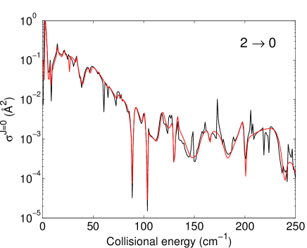
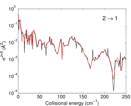
Figure 1: Partial cross sections (for total angular momentum $J=0$) for the N₂H⁺ molecule in collision with para-H${}_{2}(j=0)$ as a function of the collision energy (1 cm^-1 = 1.4 K) obtained from (i) 2D adiabatically reduced dimensional PES (red lines) (ii) full 4D PES and including coupling with $j=2,4$ and 6 levels of H₂ (black lines).

As it can be seen, the agreement between the two sets of data is extremely good, with differences of less than 5–10% between the two sets. The main differences are the presence of resonances in the calculations based on the 4D PES, that are not present or well reproduced when using the 2D PES. However, resonances have been shown to influence only moderately the magnitude of the rate coefficients and consequently, we believe that an accurate description of the scattering of N₂H⁺ with para–H₂ can be obtained by the simplified treatment described above.

2.2 Scattering Calculations

The main goal of this work is to determine hyperfine resolved integral cross sections and rate coefficients of ¹⁴N¹⁴NH⁺ molecules induced by collisions with H${}_{2}(j=0)$. Since the rotational structure of H₂ is neglected, the problem, in terms of scattering calculations, is equivalent to the collisional excitation of N₂H⁺ by a structureless atom.

Since the nitrogen atoms possess a non-zero nuclear spin ($I=1$), the N₂H⁺ rotational energy levels are split in hyperfine levels which are characterized by the quantum numbers $j$, $F_{1}$ and $F$. Here, $F_{1}$ results from the coupling of $\vec{j}$ with $\vec{I_{1}}$ ($\vec{F_{1}}=\vec{j}+\vec{I_{1}}$, $I_{1}$ being the nuclear spin of the first nitrogen atom) and $F$ results from the coupling of $\vec{F_{1}}$ with $\vec{I_{2}}$ ($\vec{F}=\vec{F_{1}}+\vec{I_{2}}$, $I_{2}$ being the nuclear spin of the second nitrogen atom). However, the hyperfine splitting of the N₂H⁺ levels is very small. Hence, by assuming that the hyperfine levels are degenerate, it is possible to considerably simplify the hyperfine scattering problem. Then, the integral cross sections corresponding to transitions between hyperfine levels of the N₂H⁺ molecule can be obtained from scattering nuclear spin free S-matrices using a recoupling method (Alexander & Dagdigian, 1985; Daniel et al., 2004).

We used Arthurs & Dalgarno (1960) description of the inelastic scattering between an atom and a linear molecule in order to obtain the close-coupling (CC) scattering matrix $S^{J}(jl;j^{\prime}l^{\prime})$, between rotational levels of N₂H⁺. We emphasize that in the calculation of the $S^{J}(jl;j^{\prime}l^{\prime})$ elements, the N₂H⁺ hyperfine structure is not taken into account. Inelastic cross sections between the hyperfine levels, from level $j,F_{1},F$ to level $j^{\prime},F_{1}^{\prime},F$, are subsequently obtained through (Daniel et al., 2004) :

$$\sigma_{jF_{1}F\to j^{\prime}F_{1}^{\prime}F^{\prime}} = \frac{\pi}{k^{2}_{jF_{1}F}}(2F_{1}+1)(2F_{1}^{\prime}+1)$$ (7)

$$\times(2F^{\prime}+1)\sum_{K}\left\{\begin{array}[]{ccc}F_{1}&F_{1}^{\prime}&K\\ F^{\prime}&F&I_{2}\end{array}\right\}^{2}$$

$$\times\left\{\begin{array}[]{ccc}j&j^{\prime}&K\\ F_{1}^{\prime}&F_{1}&I_{1}\end{array}\right\}^{2}P^{K}(j\to j^{\prime})$$

The $P^{K}(j\to j^{\prime})$ are the opacity tensors defined by :

$$P^{K}(j\to j^{\prime})=\frac{1}{2K+1}\sum_{ll^{\prime}}|T^{K}(jl;j^{\prime}l^{\prime})|^{2}$$ (8)

The reduced T-matrix elements (where $T=1-S$) are defined by Alexander & Dagdigian (1983):

$$T^{K}(jl;j^{\prime}l^{\prime}) = (-1)^{-j-l^{\prime}}(2K+1)\sum_{J}(-1)^{J}(2J+1)$$ (11)

$$\times\left\{\begin{array}[]{ccc}l^{\prime}&j^{\prime}&J\\ j&l&K\end{array}\right\}T^{J}(jl;j^{\prime}l^{\prime})$$

2.3 Computational details

The nuclear–spin–free $S^{J}(jl;j^{\prime}l^{\prime})$ matrix elements were calculated using the MOLSCAT program (Hutson & Green, 1994). All calculations were made using the rigid rotor approximation. The ¹⁴N¹⁴NH⁺ energy levels were computed using the rotational constants of Sastry et al. (1981). Calculations were carried out for total energies up to 500 cm^-1. Parameters of the integrator were tested and adjusted to ensure a typical precision to within 0.05 Ų for the inelastic cross sections and to within 1 Ų for the elastic cross sections. For example, at total energies of 100 and 500 cm^-1, total angular momentum $J$ up to 68 and 94 were taken into account in the scattering calculations, respectively. At each energy, channels with $j$ up to 28 were included in the rotational basis to converge the calculations for all the transitions including N₂H⁺ levels up to $j=7$. Using the recoupling technique and the stored $S^{J}(jl;j^{\prime}l^{\prime})$ matrix elements, the opacity tensors (Eq. 8) and the hyperfine–state–resolved cross sections (Eq. 7) were obtained for all hyperfine levels up to $j=7$.

From the calculated cross sections, one can obtain the corresponding thermal rate coefficients at temperature $T$ by an average over the collision energy ($E_{c}$):

$$k_{\alpha\rightarrow\beta}(T) = \left(\frac{8}{\pi\mu k^{3}_{B}T^{3}}\right)^{\frac{1}{2}}$$ (12)

$$\times\int_{0}^{\infty}\sigma_{\alpha\rightarrow\beta}\,E_{c}\,e^{-\frac{E_{c}}{k_{B}T}}\,dE_{c}$$

where $\sigma_{\alpha\to\beta}$ is the cross section from initial level $\alpha$ to final level $\beta$, $\mu$ is the reduced mass of the system and $k_{B}$ is Boltzmann’s constant.

3 Results

3.1 Hyperfine rate coefficients

Using the computational scheme described above, we have obtained inelastic cross sections for transitions between the first 64 hyperfine levels of N₂H⁺. With calculations performed up to a total energy of 500 cm^-1, we can determine the corresponding rate coefficients for temperatures up to 70 K. The complete set of (de-)excitation rate coefficients with $j,\,j^{\prime}\leq 7$ will be made available through the LAMDA (Schöier et al., 2005) and BASECOL (Dubernet, M.-L. et al., 2013) databases.

Figure 2 presents the temperature variation of the N₂H⁺– H${}_{2}(j=0)$ rate coefficients for selected $j=2,F_{1},F\to j^{\prime}=1,F_{1}^{\prime},F^{\prime}$ and $j=3,F_{1},F\to j^{\prime}=2,F_{1}^{\prime},F^{\prime}$ transitions.

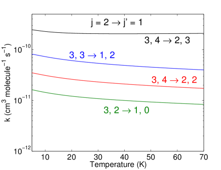
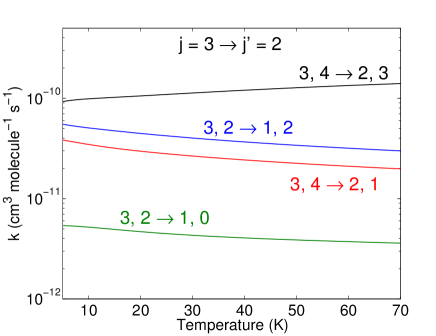
Figure 2: Temperature variation of the hyperfine resolved N₂H⁺–H₂(j=0) rate coefficients for $j=2,F_{1},F\to j^{\prime}=1,F_{1}^{\prime},F^{\prime}$ and $j=3,F_{1},F\to j^{\prime}=2,F_{1}^{\prime},F^{\prime}$ transitions.

First, one can note that the rate coefficients are weakly dependent of the temperature. This weak temperature dependance of the rate coefficients could have been anticipated, on the basis of Langevin theory for ion-neutral interactions. One can also note the relatively large magnitude of the rate coefficients ($k(T)>10^{-10}$ cm³ mol^-1 s^-1 for the dominant transitions). Usually, rate coefficients for neutral molecules such as for the isoeletronic CO molecule are of the order of magnitude of $k(T)\simeq 10^{-11}$ cm³ mol^-1 s^-1. The high magnitude of the rate coefficients can be related to the large well depth of the PES. This well depth is almost an order of magnitude larger than in the case of neutral molecules interacting with H₂. Such effect has been already observed for the HCO⁺ cation (Yazidi et al., 2014) or for the the CN^- anion (Kłos & Lique, 2011) but is absent when using He as a model for H₂. Hence, considering specifically H₂ will be of crucial importance for interstellar ions by comparison to neutral species.

In the current case, the determination of the hyperfine propensity rules is more complex than for the case of only one nuclear spin, where the usual $\Delta j=\Delta F$ propensity is observed (Ben Abdallah et al., 2012; Kalugina et al., 2012; Faure & Lique, 2012; Dumouchel et al., 2012). In fact, as explained in Daniel et al. (2004), because of the behaviour of the Wigner–6j coefficients in Eq. 7, we expect that the largest rate coefficients will satisfy (i) if $\Delta F_{1}=\Delta j$ then $\Delta F=\Delta F_{1}$, (ii) if $\Delta F_{1}=\Delta j\pm 1$ then $\Delta F=\Delta F_{1}\pm 1$. Such propensity rules were indeed found to describe, on the average, the two nuclear spins case and for the of N₂H⁺– He system (Daniel et al., 2004). However, the only well defined propensity rule is $\Delta F=\Delta F_{1}=\Delta j$ confirming that hyperfine rate coefficients cannot be accurately estimated from fine structure rate coefficients using for example the $M_{j}$ randomizing limit (Alexander, 1985) approach.

Finally, Figure 3 presents the temperature variation in N₂H⁺–H${}_{2}(j=0)$ rate coefficients for the “quasi-elastic” $j=2,F_{1},F\to j^{\prime}=2,F_{1},F^{\prime}$ transitions.

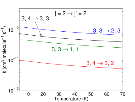
Figure 3: Temperature variation of the hyperfine resolved N₂H⁺–H${}_{2}(j=0)$ rate coefficients for $j=2,F_{1},F\to j^{\prime}=2,F_{1},F^{\prime}$ transitions.

One can notice that the order of magnitude of these “quasi-elastic” rate coefficients is similar to the pure inelastic rate coefficients. Additionally, for transitions inside a rotational level $j$, it is difficult to extract a clear propensity rule.

3.2 Comparison with He rate coefficients

It is interesting to compare the present rate coefficients with those calculated for N₂H⁺– He collisions (Daniel et al., 2005). Indeed, collisions with He are often used to model collisions with para-H${}_{2}(j=0)$ and it is generally assumed that rate coefficients with para-H${}_{2}(j=0)$ should be larger than He rate coefficients, owing to the smaller collisional reduced mass, and that the scaling factor should be $\sim$1.4 (Schöier et al., 2005). We have compared in Table 1, on a small sample, the N₂H⁺– H${}_{2}(j=0)$ and N₂H⁺– He rate coefficients at 10, 30 and 50 K.

Table 1: Selective comparison between hyperfine rate coefficients at 10, 30 and 50 K, for collisions of N₂H⁺ with para-H${}_{2}(j=0)$ (this work) and those of D05 (Daniel et al., 2005) for collisions of N₂H⁺ with He. The rates are in units of 10^-10 cm³ mol^-1 s^-1.

	10K		30K		50K
$j,F_{1},F$ $\to$ $j^{\prime},F^{\prime}_{1},F^{\prime}$	This work	D05	This work	D05	This work	D05
1, 1, 1 $\to$ 0, 1, 0	0.906	0.384	0.730	0.325	0.693	0.307
1, 2, 2 $\to$ 0, 1, 2	0.679	0.288	0.548	0.243	0.520	0.231
1, 2, 3 $\to$ 0, 1, 2	2.716	1.153	2.191	0.975	2.081	0.923
2, 1, 0 $\to$ 0, 1, 2	1.442	0.626	1.109	0.436	0.936	0.354
2, 1, 0 $\to$ 1, 2, 1	0.039	0.016	0.039	0.016	0.042	0.018
3, 2, 3 $\to$ 0, 1, 2	0.271	0.103	0.207	0.078	0.176	0.066
3, 2, 3 $\to$ 1, 0, 1	0.411	0.173	0.340	0.145	0.311	0.133
3, 2, 3 $\to$ 2, 1, 2	0.814	0.454	0.974	0.470	1.126	0.524
3, 2, 3 $\to$ 2, 3, 4	0.456	0.154	0.357	0.120	0.304	0.105
4, 3, 2 $\to$ 0, 1, 2	0.736	0.231	0.566	0.179	0.484	0.159
4, 3, 2 $\to$ 2, 1, 0	0.190	0.070	0.182	0.075	0.175	0.077
4, 3, 2 $\to$ 3, 2, 1	0.559	0.226	0.687	0.322	0.837	0.405
4, 3, 2 $\to$ 3, 3, 3	0.556	0.198	0.479	0.182	0.418	0.167

As one can see, significant differences exist between the present and the previous results. The present data differ by up to a factor of $\sim$ 3 from the previous results, the new results being systematically larger than the previous ones. Hence, the scaling factor is clearly different from 1.4 and the ratio varies with both the temperature and the transition considered.

Low collisional energies cross sections are very sensitive to the shape and depth of the PES well. It is then not surprising to see significant differences between the two collisional systems at low temperature. It could have been anticipated that scattering studies involving He as the perturber and as a representative of molecular H₂ are questionable in the case of molecular ions. As previously discussed, this is a consequence of the difference of polarizabilities with either H₂ or He.

4 Astrophysical applications

4.1 Model

As stated in Sect. 3.2, the current H₂ rate coefficients differ significantly from the previously available rate coefficients from Daniel et al. (2005), that considered He as a collisional partner. Since these rate coefficients were the only available data until now, they were used in many astrophysical studies. Most of the time, a scaling factor of 1.4 was used to emulate the H₂ rate coefficients. As discussed in the previous section, this factor leads to an underestimate of the actual values of the H₂ rate coefficients. More recently, Bizzocchi et al. (2013) used a scaling relationship based on the HCO⁺– H₂ and HCO⁺– He rate coefficients. The correction applied thus ranged from factors of 1.4 and 3.2 depending on the transition considered, with a ratio of $\sim$2.3 applied to the transitions with $\Delta j=1$ and $j\leq 4$. Given the current results, this scaling procedure gives a better estimate of the H₂ rate coefficients than simply assuming a constant 1.4 value.

In order to highlight the impact of the new rate coefficients on the interpretation of the N₂H⁺ observations, we performed a few radiative transfer calculations for physical parameters (i.e. gas density, temperature, …) and N₂H⁺ abundances typical of dark clouds conditions. These calculations are based on the numerical code described in Daniel & Cernicharo (2008): the radiative transfer is solved exactly and includes the line overlap between the hyperfine transitions. Additionally, the N₂H⁺ energy structure and line frequencies are obtained from the spectroscopical constants of Caselli et al. (1995) and Pagani et al. (2009). The line strengths and Einstein coefficients are obtained from the CDMS database (Müller et al., 2005). In Fig. 4, we compare the line intensities, integrated over frequency, for the $j=1-0$ and $3-2$ lines, and for radiative transfer calculations based either on the He or H₂ rate coefficients. For the purpose of the comparison, we made the choice to use the antenna temperature scale, noted $T_{A}^{*}$. In the figure, we give the ratio of the results based on the H₂ rate coefficients over the results obtained with the He ones, scaled by a factor 1.4. In order to perform the calculations, we assumed a static and homogeneous spherical cloud of diameter 3’ at a distance of 100 pc. We fixed the gas temperature at $T=10$ K and then varied the H₂ density in the range $10^{4}<$ $n$(H₂) $<10^{7}$ cm^-3, and the N₂H⁺ abundance in the range $10^{-11}<$ $\chi$(N₂H⁺) $<10^{-8}$ .

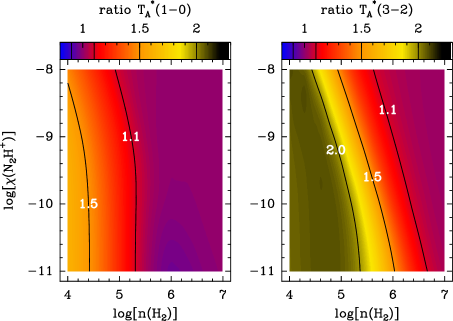
Figure 4: Ratio of the $j=1-0$ (left panel) and $j=3-2$ (right panel) integrated intensities obtained with the H₂ and He rate coefficients. These ratios are given for a uniform spherical cloud at $T=10$ K and by varying both the H₂ density and N₂H⁺ abundance.

From this figure, it appears that between the two sets of rate coefficients, the line intensities can show variations as large as a factor $\sim$2. As discussed in Sect. 3.2, this factor is similar to the difference that is obtained on average between the two sets of rate coefficients. Note that the differences are the largest at low N₂H⁺ column densities (i.e. low $n$(H₂) and/or $\chi$(N₂H⁺)), since for the highest values, both the $j=1-0$ and $3-2$ lines tend to thermalize. As an example, considering the $j=1-0$ line, we see in Fig. 4 that the integrated intensity ratio is $\sim$1 for densities $n$(H₂) $\geq$ $2\,10^{5}$ cm^-3. Finally, it can be seen in Fig. 4 that there is a differential effect introduced by the rate coefficients on the $j=1-0$ and $3-2$ line intensities. Indeed, over the conditions spanned by the current grid of models, we can see that the effect is systematically larger for the $j=3-2$ line by comparison to the $j=1-0$ line. In practice, this differential effect implies that in any astrophysical application, switching from the He rate coefficients to the H₂ rate coefficients will require to modify the estimate of both the H₂ density and the N₂H⁺ abundance, and not solely one of these parameters. In order to emphasize this point, we considered the $j=1-0$ and $3-2$ line intensities obtained with the H₂ rate coefficients and for the parameters $n$(H₂) = 2 $\times$ 10⁵ cm^-3 and $\chi$(N₂H⁺) = 1 $\times$ 10^-10. Subsequently, by using the He rate coefficients, we determined the value of $n$(H₂) and $\chi$(N₂H⁺) which enable to obtain similar line intensities for these two radiative transitions. The value of the H₂ density and N₂H⁺ abundance are determined by minimizing the quantity :

$$d=\sqrt{\left(\frac{T_{\textrm{He}}(1-0)}{T_{\textrm{H}_{2}}(1-0)}-1\right)^{2}+\left(\frac{T_{\textrm{He}}(3-2)}{T_{\textrm{H}_{2}}(3-2)}-1\right)^{2}}$$ (13)

where $T_{\textrm{H}_{2}}$ and $T_{\textrm{He}}$ stands for the integrated intensities obtained respectively with the H₂ and scaled He rate coefficients. In Fig. 5, the value of the distance $d$ is reported as a function of $n$(H₂) and $\chi$(N₂H⁺). It appears that the $j=1-0$ and $3-2$ line intensities obtained with the H₂ rate coefficients can be reproduced with the He rate coefficients by varying both $n$(H₂) and $\chi$(N₂H⁺) by factors of 2. Indeed, the minimum of $d$ is obtained for $n$(H₂) = $4\,10^{5}$ cm^-3 and $\chi$(N₂H⁺) = $5\,10^{-11}$.

Hence, using the He rate coefficients will induce an overestimation of the H₂ density and an underestimation of the N₂H⁺ abundance. Given the variations in magnitude of the rate coefficients between the two sets of rate coefficients, we can expect that a factor $\sim$2 will be typical of the modifications induced by the new set of rates on $n$(H₂) and $\chi$(N₂H⁺).

4.2 LDN 183

Since kinetic temperature has also an impact on the excitation conditions but has to be kept realistic, we revisited a well-known and modelled case, LDN 183, which was previously analysed with the hyperfine collisional rates computed with He (Pagani et al., 2007). The goal is to estimate the magnitude of the changes in a real case. We did not attempt to recompute the best possible fit to the data but only a plausible fit by eye to gauge the magnitude of the changes. With the former core properties as listed in Pagani et al. (2007), Table 2 (best model), all the modelled lines are stronger than observed with the new collision rates, as expected from the model runs described above. We tried to vary separately the kinetic temperature, the density profile and the N₂H⁺ abundance and found no convincing solution, again confirming the results discussed above. A workable solution consisted in lowering the temperature in the core, replacing the 7 K constant value by a gradient from 6 to 7 K, lowering the density by 20 % in the layers at temperature at 6.5 K or above and increasing the N₂H⁺ abundance by a factor 2 in the central two layers. Globally, the N₂H⁺ column density decreases by a factor 8 % (inner core) to 20 % for the outer core. The N₂H⁺ $j=1-0$ line being quite optically thick in LDN 183 (6 out of the 7 distinguishable hyperfine components have identical intensity towards the central position, instead of the 3:5:7 ratio observed in optically thin cases), the sensitivity of the results to the new collisional coefficients is not as dramatic as one can expect in an optically thin case but the model is more accurate and the temperature is a new low record (a temperature of 5.5 K has been advocated in the case of LDN 1544 from NH₃ interferometric observations, Crapsi et al. 2007). This temperature variation impacts also the dust temperature estimate (dust and gas are thermally coupled at n(H₂) = 1 $\times$ 10⁶ cm^-3) and consequently the dust properties.

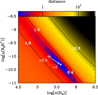
Figure 5: Comparison of the intensities predicted with the H₂ and He rate coefficients. The comparison is performed by mean of the distance $d$ defined in the text. By considering a reference model computed with the H₂ rate coefficients and with $n$(H₂) = $2\,10^{5}$ cm^-3 and $\chi$(N₂H⁺) = $10^{-10}$, we represent in this figure the optimum values for both $n$(H₂) and $\chi$(N₂H⁺), i.e. the minimum of $d$, which enables to reproduce the reference model with the He rate coefficients.

5 Conclusion

We have used quantum scattering calculations to investigate rotational energy transfer for collisions between the N₂H⁺ and para-H${}_{2}(j=0)$ molecules. The calculations were based on a new 4D potential energy surface that is then transform into a 2D adiabatically reduced dimensional PES. Rate coefficients for transitions involving the lowest hyperfine levels of the N₂H⁺ molecule were determined for temperatures ranging from 5 to 70 K. The $\Delta j=\Delta F_{1}=\Delta F$ propensity rule is found for these hyperfine transitions.

The comparison of the new N₂H⁺– H₂ rate coefficients with previously calculated N₂H⁺– He rate coefficients shows that significant differences exist. In particular, the new H₂ rate coefficients are systematically larger than the rates with He, the scaling factor being around $\sim$ 3.

The consequences for astrophysical models were also evaluated. We have performed a new set of radiative transfer calculations for physical parameters and N₂H⁺ abundances typical of dark cloud conditions. The line intensities of the simulated spectra, obtained using the new rate coefficients, are significantly larger than the ones predicted from the He rate coefficients; the factor could be as large as a factor $\sim$2 and in particular, it depends on the radiative transition. Additionally, a test on a real case (LDN 183) shows that the new rate coefficients will lead to reconsideration of the estimate of all the three: the H₂ density, the gas kinetic temperature and the N₂H⁺ abundance in cold molecular clouds.

References

- Alexander (1985) Alexander M. H., 1985, Chem. Phys., 92, 337
- Alexander & Dagdigian (1983) Alexander M. H., Dagdigian P. J., 1983, J. Chem. Phys., 79, 302
- Alexander & Dagdigian (1985) Alexander M. H., Dagdigian P. J., 1985, J. Chem. Phys., 83, 2191
- Arthurs & Dalgarno (1960) Arthurs A. M., Dalgarno A., 1960, Proc. R. Soc. A, 256, 540
- Ben Abdallah et al. (2012) Ben Abdallah D., Najar F., Jaidane N., Dumouchel F., Lique F., 2012, mnras., 419, 2441
- Bizzocchi et al. (2013) Bizzocchi L., Caselli P., Leonardo E., Dore L., 2013, A&A, 555, A109
- Caselli et al. (1995) Caselli P., Myers P. C., Thaddeus P., 1995, ApJL, 455, L77
- Crapsi et al. (2007) Crapsi A., Caselli P., Walmsley M., Tafalla M., 2007, A&A, 470, 221
- Daniel & Cernicharo (2008) Daniel F., Cernicharo J., 2008, A&A, 488, 1237
- Daniel et al. (2004) Daniel F., Dubernet M.-L., Meuwly M., 2004, J. Chem. Phys., 121, 4540
- Daniel et al. (2005) Daniel F., Dubernet M.-L., Meuwly M., Cernicharo J., Pagani L., 2005, mnras., 363, 1083
- Dubernet, M.-L. et al. (2013) Dubernet, M.-L. et al., 2013, A&A, 553, A50
- Dumouchel et al. (2012) Dumouchel F., Kłos J., Toboła R., Bacmann A., Maret S., Hily-Blant P., Faure A., Lique F., 2012, J. Chem. Phys., 137, 114306
- Dunning (1989) Dunning T. H., 1989, J. Chem. Phys., 90, 1007
- Faure & Lique (2012) Faure A., Lique F., 2012, mnras., 425, 740
- Green (1975a) Green S., 1975a, J. Chem. Phys., 62, 2271
- Green (1975b) Green S., 1975b, ApJ., 201, 366
- Hampel et al. (1992) Hampel C., Peterson K. A., Werner H.-J., 1992, Chem. Phys. Lett., 190, 1
- Havenith et al. (1990) Havenith M., Zwart E., Leo Meerts W., Ter Meulen J. J., 1990, J. Chem. Phys., 93, 8446
- Hily-Blant et al. (2008) Hily-Blant P., Walmsley M., Pineau Des Forêts G., Flower D., 2008, A&A, 480, L5
- Hutson & Green (1994) Hutson J. M., Green S., 1994. molscat computer code, version 14 (1994), distributed by Collaborative Computational Project No. 6 of the Engineering and Physical Sciences Research Council (UK)
- Indriolo et al. (2013) Indriolo N., Neufeld D., Seifahrt A., Richter M. J., 2013, ApJ, 764, 188
- Kalugina et al. (2012) Kalugina Y., Lique F., Kłos J., 2012, mnras., 422, 812
- Keto & Caselli (2008) Keto E., Caselli P., 2008, ApJ, 683, 238
- Kłos & Lique (2011) Kłos J., Lique F., 2011, mnras., 418, 271
- Lee et al. (2001) Lee C. W., Myers P. C., Tafalla M., 2001, ApJS, 136, 703
- Lemme et al. (1995) Lemme C., Walmsley M., Wilson T. L., Muders D., 1995, A&A, 302, 509
- Lique et al. (2008) Lique F., Toboła R., Kłos J., Feautrier N., Spielfiedel A., Vincent L. F. M., Chałasiński G., Alexander M. H., 2008, A&A, 478, 567
- Müller et al. (2005) Müller H. S. P., Schlöder F., Stutzki J., Winnewisser G., 2005, Journal of Molecular Structure, 742, 215
- Owrutsky et al. (1986) Owrutsky J. C., Guderman C. S., Martner C. C., Tack L. M., Rosenbaum N. H., Saykally R. J., 1986, J. Chem. Phys., 84, 605
- Pagani et al. (2007) Pagani L., Bacmann A., Cabrit S., Vastel C., 2007, A&A, 467, 179
- Pagani et al. (2012) Pagani L., Bourgoin A., Lique F., 2012, A&A, 548, L4
- Pagani et al. (2013) Pagani L., Lesaffre P., Jorfi M., Honvault P., González-Lezana T., Faure A., 2013, A&A, 551, 38
- Pagani et al. (2005) Pagani L., Pardo J. R., Apponi A. J., Bacmann A., Cabrit S., 2005, A&A, 429, 181
- Pagani et al. (2009) Pagani L. et al., 2009, A&A, 494, 623
- Sastry et al. (1981) Sastry K. V. L. N., Helminger P., Herbst E., De Lucia F. C., 1981, Chemical Physics Letters, 84, 286
- Schöier et al. (2005) Schöier F. L., van der Tak F. F. S., van Dishoeck E. F., Black J. H., 2005, A&A, 432, 369
- Scribano et al. (2012) Scribano Y., Faure A., Lauvergnat D., 2012, J. Chem. Phys., 136, 094109
- Tafalla et al. (2002) Tafalla M., Myers P. C., Caselli P., Walmsley C. M., Comito C., 2002, ApJ., 569, 815
- Walker et al. (2014) Walker K. M., Yang B. H., Stancil P. C., Balakrishnan N., Forrey R. C., 2014, ArXiv e-prints
- Watts et al. (1993) Watts J. D., Gauss J., Bartlett R. J., 1993, J. Chem. Phys., 98, 8718
- Werner et al. (1989) Werner H.-J., Follmeg B., Alexander M. H., Lemoine D., 1989, J. Chem. Phys., 91, 5425
- Willacy et al. (1998) Willacy K., Langer W. D., Velusamy T., 1998, ApJ, 507, L171
- Yazidi et al. (2014) Yazidi O., Ben Abdallah D., Lique F., 2014, mnras., 441, 664
- Zeng et al. (2011) Zeng T., Li H., Le Roy R. J., Roy P.-N., 2011, J. Chem. Phys., 135, 094304