On the structure and evolution of planets and their host stars – effects of various heating mechanisms on the size of giant gas planets

Abstract

It is already stated in the previous studies that the radius of the giant planets is affected by stellar irradiation. The confirmed relation between radius and incident flux depends on planetary mass intervals. In this study, we show that there is a single relation between radius and irradiated energy per gram per second ($l_{-}$), for all mass intervals. There is an extra increase in radius of planets if $l_{-}$ is higher than 1100 times energy received by the Earth ($l_{\oplus}$). This is likely due to dissociation of molecules. The tidal interaction as a heating mechanism is also considered and found that its maximum effect on the inflation of planets is about 15 per cent. We also compute age and heavy element abundances from the properties of host stars, given in the TEPCat catalogue (Southworth 2011). The metallicity given in the literature is as [Fe/H]. However, the most abundant element is oxygen, and there is a reverse relation between the observed abundances [Fe/H] and [O/Fe]. Therefore, we first compute [O/H] from [Fe/H] by using observed abundances, and then find heavy element abundance from [O/H]. We also develop a new method for age determination. Using the ages we find, we analyse variation of both radius and mass of the planets with respect to time, and estimate the initial mass of the planets from the relation we derive for the first time. According to our results, the highly irradiated gas giants lose 5 per cent of their mass in every 1 Gyr.

1 Introduction

The main difference between planets and stars is that stars yield energy they radiate from their nuclear fuel, but fusion reactions do not effectively occur in core of the planets. This difference leads us to consider structures of planets and stars as if they are completely different. However, the fact that both groups obey hydrostatic equilibrium makes these objects similar in some respects. Although direct light from the planets is not (or very little) received, their orbital parameters, mass ($M_{\rm p}$) and radius ($R_{\rm p}$) are found for many systems. These parameters allow us to assess the courses influencing hydrostatic equilibrium, so that eventually radius becomes very large in many cases. The aim of this study is to consider planet and host star interaction, and to assess the basic mechanisms responsible for the excess in radius of the transiting giant gas planets. The effective mechanisms we consider are irradiation, tides, molecular dissociation, cooling and evaporation.

The main scientific motivation behind the planetary research arises from our interest if there is any form of life that exists somewhere else in the Universe, other than Earth. Life has not been discovered yet in another planetary system, but there are very good candidates taking place in the habitable zone. Such a discovery will change our understanding of the Universe forever. Maybe life is rule rather than exception. The details of conditions in such planetary systems depend on the dynamics of planets. In this regard, the data of all kinds are very important.

Thanks to the Kepler (Borucki et al. 2009; Koch et al. 2010) and CoRoT (Michel et al. 2006; Auvergneş et al. 2009) missions, huge amount of data on the basic properties of planets are accessible now. In addition to them, there are several ground-based projects for discovery of the new planetary systems: HARPS (Mayor et al. 2003), HAT (Bakos et al. 2002), HATnet (Bakos et al. 2004), KELT (Pepper et al. 2012; Siverd et al. 2012), OGLE (Udalski 2003), Qatar (Alsubai et al. 2013), SuperWASP (Street et al. 2003), TrES (Alonso et al. 2004), WASP (Pollacco et al. 2006), WTS (Cappetta et al. 2012), XO (McCullough et al. 2005).

Number of confirmed planets in 1036 host stars is given as 1706 (Akeson et al. 2013; exoplanetarchive.ipac.caltech.edu), at the time of writing this paper. Some of these systems are multiplanetary. Their number is 442. According to the data in TEPCat, the mass of the planets ranges 1.017 M${}_{\oplus}=$ 0.0032 M_J (KOI-314 c; Kipping et al. 2014) to 69.9 M_J (LHS 6343 b; Johnson et al. 2011). The upper mass range consists of brown dwarfs. With its mass of 10.52 M_J (Maxted et al. 2013), WASP-18b is considered to be the most massive planet below the brown dwarf regime ($M_{\rm p}>13{M}_{\rm J}~{})$. The sizes of planets range 0.296 R${}_{\oplus}=$ 0.027 R_J (Kepler-37 b; Barclay et al. 2013) to 2.09 R_J (WASP-79 b; Smalley et al. 2012). The lower mass interval for the inflated planets is about 0.35–0.4 M_J. Their sizes nearly take the upper part of the radius range, 0.8–1.4 R_J.

Luminosity of a star is mainly a measure of how hot its nuclear core is. Its radius, however, is also a sensitive function of how energy is efficiently transferred as much as how much energy is produced. Therefore, radius of a star depends on structure of its inner and outer regions. Metallicity significantly affects structure of these regions. Therefore, we develop a new simple method to find the age of the host stars as a function of metallicity, in addition to mass and radius (see Section 3.2).

The only observed parameter that reflects the internal structure of a giant gas planet with known mass is its radius. It has already been confirmed in many studies that the radii of planets are related with the incident flux (see, e.g. Burrows et al. 2000; Demory & Seager 2011). This means that the atmosphere and the most outer regions are effectively heated by the energy released by the host star. The giant gas planets Jupiter and Saturn in our Solar system have nearly the minimum radii in comparison with their counterparts because they are old enough to cool down but not sufficiently heated by the Sun.

The equation of state (EOS) for planets (Fortney & Nettelmann 2010) is much more complicated than stellar EOS. For massive main-sequence (MS) stars, the pressure against the gravity is essentially the ideal gas pressure. It is well known that low-mass stars, are in average cooler and denser than high-mass stars. For these stars, non-ideal effects become important because ionized particles feel the fields of surrounding charged particles. In comparison, planets are much cooler and denser than the low-mass stars. Therefore, planets EOS is much more complicated due to non-ideal interactions between the particles they consist of. This is one of the major obstacles that limits our better understanding of planetary structure and evolution.

The radius of a star for a given mass essentially depends on distribution of number of particles and temperature throughout its interior. Both of these parameters are functions of chemical composition and time (see, e.g. Baraffe, Chabrier & Barman 2008; Howe, Burrows & Verne 2014; Lopez & Fortney 2014; Howe, Burrows & Verne 2014). The similar situation is also valid for gas giant planets, although star and planet interiors are very different. Chemical composition changes from star to star, however, it seems that chemical composition plays a very important role in planets (see Section 4.5). This may be another important obstacle that limits our understanding of the structure and evolution of planets.

The particles in the outer regions of the giant gas planets are assumed to be in molecular form (Bilger, Rimmer & Helling 2013; Miguel & Kaltenegger 2014). However, some irradiated planets have so high equilibrium temperature, which is the blackbody temperature of a planet heated only by its parent star, the form of the material may be atomic rather than the molecular. Since gas pressure is primarily a function of number of particles, different material forms imply different planetary sizes (see Section 4.3).

One of the most efficient heating mechanisms responsible from inflated planets is tidal interaction between planet and its host star (Wu 2005; Jackson, Greenberg & Barnes 2008; Liu, Burrows & Ibgui et al. 2008). This interaction cause to convert orbital energy to the internal energy of the most outer regions of the planet (see Section 4.2).

In this paper, we consider which and how mechanisms are influencing the size of gas giant planets. The paper is organized as follows. In Section 2, the basic observational properties of the transiting planets and their host stars are presented. Section 3 is devoted to the methods we develop for determination of the metallicity and age of the host stars. In Section 4, we in detail consider how various mechanisms affect the planetary size. Finally, in Section 5, we draw our conclusions.

2 Basic properties of planets and their host stars

The data are taken from the TEPCat data base (www.astro.keele.ac.uk/jkt/tepcat/) for the transiting planetary systems in 2014 January 6, and listed in the online Table A1. In Fig. 1, the radii of planets are plotted with respect to the planetary mass. For low-mass range there is a nearly linear relation between mass and radius. About 1 M_J, the relation changes and radius is essentially independent of mass, in particular for the range 0.4–4.5 M_J. For this range the average radius is about 1.28 R_J. The minimum and maximum radii are 0.775 R_J of WASP-59 b (Hébrard et al. 2013) and 2.09 R_J of WASP-79 b (Smalley et al. 2012), respectively. Both of these planets have slightly lower mass than Jupiter: masses of WASP-59 b and WASP-79 b are 0.863 M_J and 0.90 M_J, respectively. The radius of Jupiter is in the lower part of the range.

Eccentricity of some planetary systems in TEPCat catalogue is given as zero, but their eccentricities updated by Knutson et al. (2014) are non-zero. In Table A1, the updated eccentricities, very important for tidal interaction (see Section 4.2), are listed.

Radius of a polytropic model for planets is given as $R_{\rm p}\propto M_{\rm p}^{1-1/n}$, where $n$ is polytropic index. The best representation of internal structure of intermediate mass planets is with $n=1$, which gives radius as independent of $M$ (Burrows & Liebert 1993). This simple case allows us to construct toy models for the giant gas planets. More realistic models are given and discussed in Guillot & Gautier (2014).

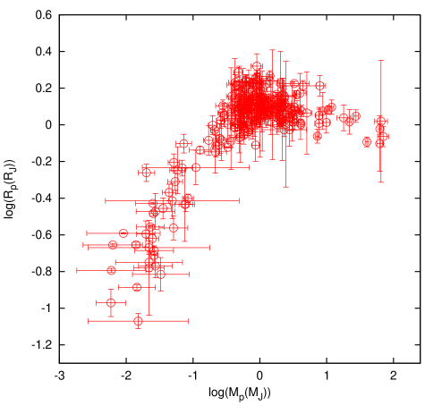
Figure 1: Planetary radius with respect to planetary mass.

We consider the planetary radii in four groups, according to their masses. The mass range of the most inflated planets is 0.4–4.5 M_J. Mass of the other two groups are above and below this range. This study essentially deals with the planets with $M_{\rm p}>0.4$ M_J.

The effective temperature of the host stars range from 4550 to 7430 K. The most of them are MS stars, with a limited number of more evolved stars. Their sizes are in between 0.694 and 6.20 R_☉. The mass range of the host stars is 0.75–1.57 M_☉. Age of these planetary systems are found from mass, radius and metallicity of the host stars. The method is explained in Section 3.

3 Estimated heavy element abundance and age for the planetary systems

3.1 Estimated heavy element abundance

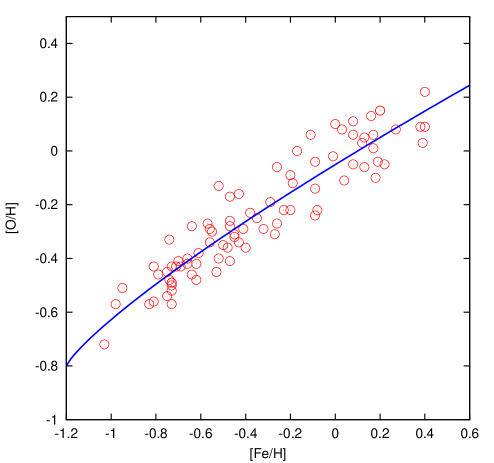
Figure 2: $[{\rm O/H}]$ is plotted with respect to $[{\rm Fe/H}]$. The data are taken from Edvardsson et al. (1993). The solid line represents the fitting curve $0.645([{\rm Fe/H}]+1.2)^{0.82}-0.8$.

Figure 3: $Z_{\rm Fe}$ is plotted with respect to $Z_{\rm O}$ for the planetary systems. The solid line shows the fitting curve $73.4Z_{\rm O}^{2}$.

Figure 4: $Z_{\rm O}$ is plotted with respect to $[{\rm Fe/H}]$ for the planetary systems. The solid line is for the derived fitting curve $0.00165([{\rm Fe/H}]+1.916)^{3}+0.0037$.

MS lifetime and hence age of a star depend on its metallicity ($Z$) and mass ($M$). The higher the metallicity is, the greater the age is. Therefore, observational constraint to $Z$ is needed for a precise age computation. $[{\rm Fe/H}]$ abundance is customarily considered as a representative of the total heavy element abundance $Z$ assuming all the heavy element species are enhanced in the same amount relative to the solar abundance. However, oxygen is the most abundant heavy element in normal stars and there is an inverse relation between $[{\rm Fe/H}]$ and $[{\rm O/Fe}]$ abundances, according to the findings of Edvardsson et al. (1993, see their fig. 15a-1). They studied solar neighbourhood stars and derived chemical abundances of 189 stars. They find that [O/Fe] is about 0.2 dex for the metal-poor stars ($[{\rm Fe/H}]\approx-0.2$ dex), and it is about $-0.2$ dex for the metal-rich stars ($[{\rm Fe/H}]\approx 0.2$ dex). Using their data, $[{\rm O/H}]$ is plotted with respect to $[{\rm Fe/H}]$ in Fig. 2. The fitting formula for $[{\rm O/H}]$ is found as

$$[{\rm O/H}]=0.645([{\rm Fe/H}]+1.2)^{0.82}-0.8.$$ (1)

Then, we find $Z_{\rm O}$ of the host stars from $[{\rm O/H}]$. We assume a linear relation between total heavy element and oxygen abundances:

$$Z_{\rm O}=10^{[\rm O/H]}{\rm Z_{\sun}}.$$ (2)

In Fig. 3, $Z_{\rm Fe}=10^{[\rm Fe/H]}{\rm Z_{\sun}}$ directly derived from $[{\rm Fe/H}]$ is plotted with respect to $Z_{\rm O}$. For low $Z$, the difference between $Z_{\rm Fe}$ and $Z_{\rm O}$ is not very large. For high $Z$, however, the difference is extremely large. While the maximum value of $Z_{\rm Fe}$ is about 0.05, the maximum value of $Z_{\rm O}$ is about half of this value, 0.025. According to the fitting curve $Z_{\rm Fe}\propto Z_{\rm O}^{2}$, or $Z_{\rm O}\propto Z_{\rm Fe}^{1/2}$.

In Fig. 4, $Z_{\rm O}$ is plotted with respect to [Fe/H]. One can use this figure to find more realistic metallicity of any star if its [Fe/H] is observed.

The metallicity of the planetary systems is between $Z_{\rm O}=0.009$ and $0.026$. Its mean value is about 0.0169. Uncertainty in metallicity is mainly due to relation between [O/H] and [Fe/H]. The mean uncertainty in [O/H] is about 0.1 dex and this implies a maximum uncertainty in $Z_{\rm O}$ about 25 per cent. $Z_{\rm O}$ and its uncertainty are listed in Table A1.

3.2 Age estimation

Radius and luminosity of a star are steadily increasing during the MS evolutionary phase until the totally collapse after the hydrogen fuel is depleted near the terminal-age MS (TAMS). These are most convenient stellar parameters among non-asteroseismic constraints for age determination. Only for few host stars we have asteroseismic constraints and their ages are available in the literature (see Table 1). We have developed a new method for age determination of these stars within the mass range 0.75–1.6 M_☉, based on stellar mass, radius and metallicity.

Stellar evolution grids are obtained by using the ANKİ stellar evolution code for different composition. These models are the same models used in Yıldız et al. (2014a), Yıldız, Çelik Orhan & Kayhan (2014b) and Yıldız (2014).

The EOS routines of ANKİ take into account Coulomb interaction and solve the Saha equation (Yıldız & Kızıloğlu 1997). The radiative opacity is derived from OPAL tables (Iglesias & Rogers 1996), supplemented by the low temperature tables of Ferguson et al. (2005). Nuclear reactions are taken from Angulo et al. (1999) and Caughlan & Fowler (1988). The standard mixing length theory is employed for the convection (Böhm-Vitense 1958).

The reference models are computed with solar values. From calibration of solar luminosity and radius we find that $X_{\sun}=0.7024$, $Z_{\sun}=0.0172$. The heavy element mixture is taken as the solar mixture given by Asplund et al. (2009). The solar value of the convective parameter $\alpha$ for ANKİ  is $1.98$.

According to our stellar evolution understanding, radius ($R$) and luminosity ($L$) of a model are minimum around zero-age-MS (ZAMS) and become maximum near TAMS. The TAMS values of $R$ and $L$ are approximately 1.5 and 2 times greater than the ZAMS values, respectively, for the entire mass interval: $R_{\rm TAMS}\approx 1.5R_{\rm ZAMS}$ and $L_{\rm TAMS}\approx 2L_{\rm ZAMS}$.

We consider radius as a function of stellar mass, metallicity and age. The difference ($\Delta R$) between the present radius ($R(t)$) and R_ZAMS is then a measure of the relative age ($t_{\rm rel}$), defined as

$$t_{\rm rel}=\frac{t}{t_{\rm TAMS}},$$ (3)

where $t$ is age. If $\Delta R=R(t)-R_{\rm ZAMS}$ is about 0.5 R_ZAMS then $t_{\rm rel}\approx 1$ and $t\approx t_{\rm TAMS}$. If $\Delta R$ is very small then $t_{\rm rel}\approx 0$ and $t\approx t_{\rm ZAMS}$.

In order to find the increase in radius, R_ZAMS is needed. There is no single relation between mass and radius in the mass range we deal with. For the models with solar composition, one can adopt two different relations for $M_{\rm t}>M_{\rm t\sun}$ and $M_{\rm t}<M_{\rm t\sun}$. $M_{\rm t\sun}$ is the transition mass and about $1.3$  M_☉ for the solar composition. We obtain

$$\frac{{R}_{\rm ZAMS}}{{\rm~{}R}_{\sun}}=0.504\left(M/{\rm~{}M}_{\sun}\right)^{2.02}+0.384$$ (4)

if $M$ is less than $M_{\rm t\sun}$, otherwise,

$$\frac{{R}_{\rm ZAMS}}{{\rm~{}R}_{\sun}}=1.294\log(M/{\rm~{}M}_{\sun})^{0.267}.$$ (5)

For arbitrary $Z$, $M_{\rm t}(Z)=M_{\rm t\sun}(Z/{\rm Z_{\sun}})^{0.22}$.

From model computations we confirm that increase in radius is proportional to $t_{\rm rel}^{3/2}$:

$$\frac{R(t)}{{\rm~{}R}_{\sun}}=\frac{{R}_{\rm ZAMS}}{{\rm~{}R}_{\sun}}+a(M,Z)t_{\rm rel}^{3/2},$$ (6)

where the coefficient $a(M,Z)$ is a function of both $M$ and $Z$. It is obtained as

$$a(M,Z)=0.114b\left(\left(\frac{M}{8.8\rm M_{\sun}}\right)^{5}+1\right)+(0.222-b)\left(\frac{M}{\rm M_{\sun}}\right)$$ (7)

where $b$ is a function of $Z$ and found as

$$b(Z)=\frac{5.297}{3.139+(Z/{\rm Z_{\sun}})^{4.6}}.$$ (8)

If we are given radius, mass and $Z$, $t_{\rm rel}$ can be found by using equation (6), provided that R_ZAMS is known. Then, age can be computed from equation (3). We must keep in mind that $t_{\rm TAMS}$ is, beside $M$, also a function of $Z$:

$$t=t_{\rm rel}t_{\rm TAMS}(M,Z).$$ (9)

From comparison of models with different $Z$, we find that

$$t=t_{\rm rel}t_{\rm TAMS}(M,{\rm Z_{\sun}})\left(\frac{Z}{\rm Z_{\sun}}\right)^{0.59}.$$ (10)

The MS lifetime we derive is as

$$t_{\rm TAMS}(M,Z=\rm Z_{\sun})=\frac{9.7\times 10^{9}}{(M/{\rm~{}M}_{\sun})^{4.14}}\left(0.972+0.0073\left(\frac{M}{{\rm~{}M}_{\sun}}\right)^{8.4}\right).$$ (11)

The present method yields the solar age as 4.3 Gyr. This result is in very good agreement with the solar age found by Bahcall, Pinsonneault & Wasserburg (1995), 4.57 Gyr.

The ages of the planetary systems for $Z_{\rm O}$ we obtain from the application of the present method are given in Table A1. The ages range 0.3–11.1 Gyr. The mean value is about 4.2 Gyr. If we use $Z_{\rm Fe}$ in place of $Z_{\rm O}$, the upper limit for age of the host stars is about 17 Gyr, which is much larger than the adopted value of the Galactic age, given as 13.4 $\pm$ 0.8 Gyr by Pasquini et al. (2004). Uncertainty in age is about 10 per cent.

In the literature, the ages of three planetary systems from asteroseismic inferences are available. These ages and ages found in this study are listed in Table 1. The results from two methods are in very good agreement.

Table 1: Comparison of ages found in this study with the ages from asteroseismic inferences.

Star	$M$	$R$	$Z$	$T_{\rm eff}$	age	age(seis)	Ref.
	(M☉)	(R☉)		(K)	(Gyr)	(Gyr)
HD 17156	1.30	1.49	0.020	6079	2.7$\pm$0.6	2.8 $\pm$ 0.6	1
HAT-P-7	1.51	1.96	0.021	6350	1.9$\pm$0.1	2.14$\pm$ 0.26	2
”						2.21$\pm$ 0.04	3
Kepler-56	1.32	4.23	0.019	4840	3.4$\pm$0.9	3.5 $\pm$ 1.3	4

(1) Gilliland et al. (2011), (2) Christensen-Dalsgaard et al. (2010), (3) Oshagh et al. (2013), (4) Huber et al. (2013).

4 The mechanisms influencing planetary radius

4.1 Effect of incident flux

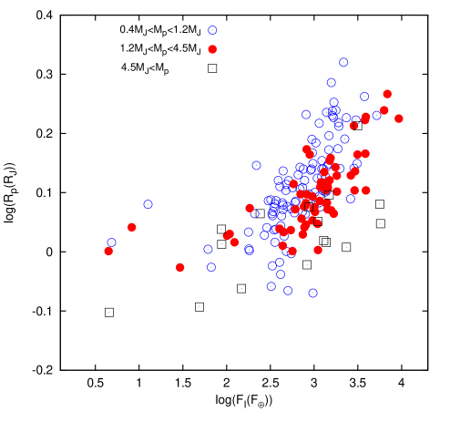
Figure 5: Planetary radius with respect to incident flux in units of incident flux at Earth for different planetary mass groups. While the circles are for the planets $0.4$ M_J $<M_{\rm p}<1.2$ M_J and the filled circles show $1.2$ M_J $<M_{\rm p}<4.5$ M_J, the squares are for $M_{\rm p}>4.5$ M_J.

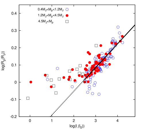
Figure 6: Planetary radius with respect to total energy received by the planet per gram per second. The fitting line is as ${(0.138\pm 0.008)\log(l_{-}/l_{0})-(0.327\pm 0.025)}$. The effect of $l_{-}$ on the radius can be given as $\Delta\log(R_{l})=0.138(\Delta\log(l_{-}/l_{0})-2.5)$

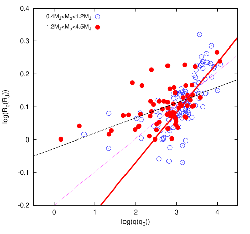
Figure 7: Planetary radius with respect to heat ($q=l_{-}t$) in units of $q_{0}=l_{0}t_{\sun}$. The solid line is the fitting line for 0.4–1.2 M_J and $\log(q/q_{0})>2.4$, ${(0.152\pm 0.014)\log(q/q_{0})-(0.374\pm 0.048)}$. The dotted line is the fitting line for 1.2–4.5 M_J and $\log(q/q_{0})>2.4$, ${(0.102\pm 0.020)\log(q/q_{0})-(0.200\pm 0.061)}$. The dashed line is also for 1.2–4.5 M_J but for full range of $\log(q)$, ${0.047\pm 0.010)\log(q/q_{0})-(0.027\pm 0.027)}$.

The effect of incident flux ($F_{\rm I}$) on the size of the planets is widely considered in many studies in the literature (see, e.g. Guillot et al. 1996; Burrows et al. 2000; Sudarsky, Burrows & Hubeny 2003; Fortney et al. 2007; Demory & Seager 2011; Weiss et al. 2013). The flux heats the outer regions of planets. This causes an increase of temperature of those regions. If the matter in the heated regions is in the gas form, then pressure increases, and therefore the gas planets expand in order to reach hydrostatic equilibrium. An alternative explanation might be that heating prevents cooling of the outer regions of giant gas planets, and therefore pressure and eventually their radii remain high.

In Fig. 5, radii of the giant planets of three mass groups are plotted with respect to the incident flux in units of flux received by Earth. The largest planets are the planets with the highest irradiated energy. We consider intermediate mass planets in two subgroups; $0.4$ M_J $<M_{\rm p}<1.2$ M_J and $1.2$ M_J $<M_{\rm p}<4.5$ M_J. The excess in radius is different for different mass groups. For a given incident flux, the intermediate mass planets have larger radius than the high-mass planets. This seems very reasonable because the temperature in the heated region is determined by energy per mass, rather than the incident flux. Excess in radius must be due to the increase in the pressure of the heated regions. The pressure is related to the total received energy per gram per second. The total energy per second received by the planet $L_{-}$ is

$$L_{-}={\rm\pi}R_{\rm p}^{2}F_{\rm I}.$$ (12)

Increase in temperature depends on how much energy is received per gram per second, i.e. on $L_{-}/M_{\rm p}$ ratio, assuming proportionality between mass of the heated region and the total planetary mass. In Fig. 6, $\log(R_{\rm p})$ is plotted with respect to logarithm of $l_{-}=L_{-}/M_{\rm p}$ in units of $l_{0}$, where $l_{0}=1.106\times 10^{-4}$ erg g^-1 s^-1 is received energy per unit mass and time by a planet with 1 M_J and 1 R_J at 1 au in our Solar system. $l_{0}$ is 0.379 times the received energy per unit mass and time by Earth ($l_{\oplus}$). The inflated planets are the planets heated about 110–190 ($\log(l_{-}/l_{0})=$2.5–2.7) times more than Earth. The intermediate and high-mass planets obey the same relation in $\log(R_{\rm p})$ and $\log(l_{-})$ diagram. Therefore, the relation between $R_{\rm p}$ and $l_{-}$ is much more explicit than the relation between $R_{\rm p}$ and $F_{\rm I}$ given in Fig. 5.

As stated above, Fig. 5 shows that the excess in radii of planets receiving the same flux depends on the planetary mass. The mean radius difference between the planets with 0.4–1.2 M_J and 1.2–4.5 M_J is about $\Delta\log(R_{\rm p}/{\rm R}_{\rm j})\approx 0.1$, for a given $F_{\rm I}$. This means the difference is about 26 per cent. In Fig. 6, however, we note that the mean radii of the planets with 0.4–1.2 M_J and 1.2–4.5 M_J are the same for a given $l_{-}$.

However, $l_{-}$ is also related with the ratio of $F_{\rm I}$ to gravity at the surface of the planets:

$$l_{-}=\frac{{\rm\pi}F_{\rm I}}{M_{\rm p}/R_{\rm p}^{2}}\propto\frac{F_{\rm I}}{g_{\rm p}}.$$ (13)

For a given value of $F_{\rm I}$, increase in radius of a planet also depends on gravitational acceleration in the expanding outer regions. The weaker the gravity is, the greater the expansion is. Perhaps, therefore the $R_{\rm p}$–$l_{-}$ relation is much more definite than the $R_{\rm p}$–$F_{\rm I}$ relation. We note that the horizontal axis of Fig. 6 also contains $R_{\rm p}$ implicitly. If we want to consistently write an expression for radius, $F_{\rm I}/M_{\rm p}$ is the alternative of $F_{\rm I}R_{\rm p}^{2}/M_{\rm p}$. For this purpose, we derive

$$\log(\frac{R_{\rm p}}{{R}_{\rm J}~{}})={({0.077\pm 0.007})\log(\frac{F_{\rm I}/{\rm F}_{\oplus}}{M_{\rm p}/M_{\rm J}})-({0.422\pm 0.048})}$$ (14)

for $\log(F_{\rm I})>2.5\log({\rm F}_{\oplus})$.

We also test if the total heat added ($q=l_{-}t$) to the planets during their lifetime has any influence on the planetary size. In Fig. 7, $R_{\rm p}$ is plotted with respect to $q$. The relation between $R_{\rm p}$ and $q$ is not strong as the relation between $R_{\rm p}$ and $l_{-}$. However, there is a small slope in the low-heat region ($q<3$).

4.2 Effect of tides

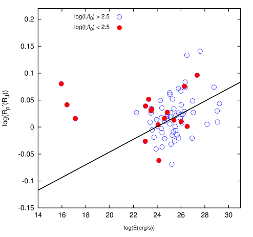
Figure 8: Planetary radius $R_{\rm p}^{\prime}$ with respect to energy rate due to tidal interaction between host star and planet in eccentric orbit. $R_{\rm p}^{\prime}$ is $R_{\rm p}-\Delta R_{l}$, where $\Delta R_{l}$ is the amount of expansion due to $l_{-}$ (see Fig. 6). The circle and filled circle are for the planets with $\log(l_{-}/l_{0})>2.5$ and $\log(l_{-}/l_{0})<2.5$, respectively. The fitted line is $(0.012\pm 0.004)\log(\dot{E}/$(erg s${}^{-1}))-(0.290\pm 0.100)$ obtained for the range $\log(\dot{E}/$(erg s${}^{-1}))>24$.

The tidal interaction between a planet and its host star may heat the planet, if the orbit is eccentric or the planet rotates asynchronously (Bodenheimer, Lin & Mardling 2001; Jackson, Greenberg & Barnes 2008). Since we do not have any information about how the planets rotate, we only consider the planetary systems with eccentric orbits. The heating mechanism in such systems is studied in, e.g. Storch & Lai (2014) and Leconte et al. (2010). We apply the heating mechanism given by Storch & Lai (2014). The rate of energy ($\dot{E}$) converted from orbital energy to the heat is

$$\dot{E}=\frac{{\rm d}E_{\rm tide}}{{\rm d}t}=2K_{\rm p}[N_{\rm a}(e)-\frac{N^{2}(e)}{\Omega(e)}]$$ (15)

where $N(e)$, $N_{\rm a}(e)$ and $\Omega(e)$ are only function of the eccentricity ($e$). They are given as

$$N(e)=\frac{1+15/2e^{2}+45/8e^{4}+5/16e^{6}}{(1-e^{2})^{6}},$$ (16)

$$N_{\rm a}(e)=\frac{1+31/2e^{2}+255/8e^{4}+185/16e^{6}+25/64e^{8}}{(1-e^{2})^{15/2}}$$ (17)

and

$$\Omega(e)=\frac{1+3e^{2}+3/8e^{4}}{(1-e^{2})^{9/2}}.$$ (18)

Expression for the other parameter $K_{\rm p}$ shown in equation (15) is as

$$K_{\rm p}=\frac{3}{2}k_{\rm 2,p}\Delta t_{\rm p}(\frac{GM^{2}_{\rm p}}{R_{\rm p}})(\frac{M_{\rm\ast}}{M_{\rm p}})^{2}(\frac{R_{\rm p}}{a})^{6}n^{2}$$ (19)

where $k_{\rm{2,p}}$, $\Delta t_{\rm p}$ and $n$ are the potential Love number of degree 2, constant time-lag for planet and the orbital mean motion, which is $2{\rm\pi}/P_{\rm orb}$, respectively. $k_{\rm{2,p}}\Delta t_{\rm p}$ is taken as $2\times 10^{-2}$–$2\times 10^{-3}$ values for giant gas planets. These equations are used for calculating energy of planet’s tidal effect (Leconte et al. 2010; Storch & Lai 2014) by adopting the upper value of $k_{\rm{2,p}}\Delta t_{\rm p}$.

The radius of the planets with eccentric orbits and $\log(l_{-}/l_{0})<2.5$ are plotted with respect to tidal energy rate in Fig. 8. In order to see net result of tides, we also plot planets with $\log(l_{-}/l_{0})>2.5$ by subtracting the excess in radius due to irradiation from the observed radius. The values of $\dot{E}$ range from $10^{16}$ to $10^{29}$ erg s^-1. The tidal interaction influences radius of a planet if $\dot{E}$ is greater than $10^{22}$ erg s^-1. The solid line is the fitted line if we assume a linear relation between $\log(R_{\rm p}^{\prime})$ and $\log(\dot{E})$. In order to make the effect of tides clearer, the planets with $\log(l_{-}/l_{0})>2.5$ and $\log(l_{-}/l_{0})<2.5$ are marked with different symbols. Since irradiation energy is effective on the planet radius if $\log(l_{-}/l_{0})>2.5$, the most inflated planets are the planets with the highest irradiated energy. The pure tidal effect might be on the planetary systems with $\log(l_{-}/l_{0})<2.5$. The maximum effect of tides seems to be about 10 per cent. The same is true for $\log(l_{-}/l_{0})>2.5$, but the maximum effect is about 15 per cent for CoRoT-2 b (Alonso et al. 2008) and WASP-14 b (Joshi et al. 2009).

4.2.1 Tidal effect and Roche lobe filling factor

The gravitational acceleration applied by the star on the inner surface of the planet ($g_{\rm\star}=GM_{\rm\star}/(a-R_{\rm p})^{2}$) is non-negligible in comparison with the self gravitational acceleration ($g_{\rm p}=GM_{\rm p}/R_{\rm p}^{2}$) plus centrifugal acceleration $g_{\rm c}=v^{2}_{\rm p}/(a-R_{\rm p})$, where $v_{\rm p}$ is the orbital speed. When the planet is at periastron, its nearest part is pulled towards the star, and therefore it gains potential energy. This potential energy is converted into kinetic energy, and later into heat when the planet travels towards the apastron. However, asynchronous rotation of planet in a circular orbit may also cause to heat the outer regions of planets.

The centrifugal acceleration at periastron is $g_{\rm cperi}=\omega^{2}_{\rm peri}a(1-e)$, where $\omega_{\rm peri}=2{\rm\pi}/P\sqrt{(1+e)/(1-e)}$. $g_{\rm\star peri}=GM_{\rm\star}/a^{2}(1-e)^{2}$ represents gravitational acceleration due to the host star at periastron. The effect of tidal interaction depends on the ratio of accelerations:

$$r_{\rm peri}=\frac{g_{\rm\star peri}}{g_{\rm p}+g_{\rm cperi}}.$$ (20)

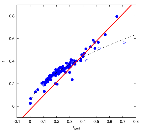
Figure 9: The Roche lobe filling factor, $f$, is plotted with respect to ratio of accelerations, $r_{\rm peri}$ (equation 20) for the gas giant planets with $0.4$ M_J $<M_{\rm p}<1.2$ M_J. There are two different relations between $f$ and $r_{\rm peri}$. The curve with dashed line is for the range $f<0.4$, and the solid line is for $f>0.4$. For some of the planetary systems, eccentricities are updated by Knutson et al. (2014). These systems are represented by circles. We note that two planets with the recent eccentricity values lie near to the dashed line.

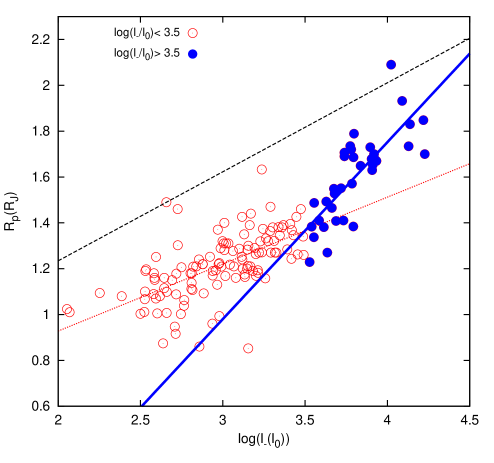
Figure 10: Planetary radius with respect to $\log(l_{-})$. The dotted and solid lines are for the ranges $\log(l_{-}/l_{0})<3.5$ and $\log(l_{-}/l_{0})>3.5$, respectively. If we consider molecular dissociation, radius of a planet is multiplied by about 33 per cent. When we multiply line equation for $\log(l_{-}/l_{0})<3.5$ (dotted line) by 1.33 we obtain the dashed line (see Section 4.3).

To confirm the effect of tidal interaction on the planetary size, the filling factor ($f$), the ratio of the planetary radius to the Roche lobe radius, is plotted with respect to $r_{\rm peri}$ in Fig. 9. The Roche lobe radius is computed by using the expression in Eggleton (1983). There are two different relations between $f$ and $r_{\rm peri}$. The transition occurs at about $f=0.35$–$0.40$. This point corresponds $\log(l_{-}/l_{0})\approx 3.5$. The curve represents the fit for $f<0.4$ and it is only an extrapolation for $f>0.4$. For the range $f>0.4$, the relation between $f$ and $r_{\rm peri}$ is linear.

4.3 Effect of molecular dissociation

In Fig. 10, the radii of giant gas planets are plotted with respect to $\log(l_{-})$. Two different $\log(l_{-})$ ranges are represented with different symbols. There is a good linear relation between planetary radius and $\log(l_{-})$ for $\log(l_{-}/l_{0})<3.5$, with a slope of 0.29. The relation changes if $\log(l_{-}/l_{0})>3.5$. There is a relatively sharp slope for the range $\log(l_{-}/l_{0})>3.5$, about 0.77. The reason for the change in the slope may be related with the structure of the heated part of the planets. We note that $T_{\rm eq}>1500$ K, when $\log(l_{-}/l_{0})>3.5$ and $T_{\rm eq}$ reaches 2700 K for some planets. $T_{\rm eq}$ values are taken from TEPCat and given in Table A1. We can expect molecular dissociation at such high temperatures. Maybe, this is the reason for the presence of two very different slopes in Fig. 10 (see below).

The most abundant species in the surface of the giant gas planets in our Solar system, namely Jupiter and Saturn, is H₂ molecules (Atreya et al. 2003). If H₂ molecules in some very hot gas planets dissociate due to various heating mechanisms, then we can expect that radii of these planets must be greater than their counterparts. We can assess the basic effect of molecular dissociation in a simple manner. Let us consider a gas made of diatomic molecules with $T$, close to but less than dissociation temperature. If the gas is heated, it will expand adiabatically and adopt a new equilibrium state so that pressure at a mass element remains constant to good approximation. The gas transforms from molecular to atomic form in the outer regions and the number density of particles ($n_{\rm f}$) is twice the initial value ($n_{\rm i}$). Then, its volume ($V$) increases. The relation between $\Delta R=R_{\rm f}-R_{\rm i}$ and $\Delta V=V_{\rm f}-V_{\rm i}$ for a spherical object can be written as

$$\frac{\Delta R}{R_{\rm i}}=\frac{1}{3}\frac{\Delta V}{V_{\rm i}}$$ (21)

If $n_{\rm f}\approx 2n_{\rm i}$, then $V_{\rm f}\approx 2V_{\rm i}$, assuming the ideal gas law is nearly satisfied in the expanding outer regions. This implies that $\Delta V=V_{\rm i}$. Then, from equation (21),

$$R_{\rm f}=R_{\rm i}+\Delta R=1.33R_{\rm i}.$$ (22)

This implies that $\Delta R$, which is the increase in radius due to increase in number of particles as a result of molecular dissociation, is $0.33R$.

If we multiply the fitted line (dotted line) in Fig. 10 by 1.33 (dashed line), then we nearly obtain the maximum effect of molecular dissociation on the planetary radius. We note that it limits almost all the data (except WASP-79 b) and there are some planets very close to this line.

4.4 Variation of planetary radius in time – effect of cooling

Interior of protoplanets are very hot. Their internal temperature decreases in time as a result of the cooling process, at a rate depending on planetary mass and irradiation energy. In this section, we consider if the effect of cooling is seen in the current data and try to determine if cooling rate also depends on the irradiated flux. To do these, we divide the planets within the mass range $0.4$ M_J $<M_{\rm p}<4.5$ M_J into four subgroups according to their $l_{-}$. The properties of these subgroups are given in Table 2. $\ln(R_{\rm p})$ is plotted with respect to age in Fig. 11 for these subgroups. Also shown in this figure are the fitted lines. The slopes of these lines are different for different $l_{-}$ intervals and decrease as $l_{-}$ reduces.

The alternative expression to the time variation of radius is that planetary radius shows extra dependence on stellar effective temperature, for example. High effective temperature of host stars means high energetic photons throughout irradiation energy. Maybe, heating also depends on energy content of photons as well as total irradiation flux. However, we see a similar time variation also for planetary mass (see Fig. 12). This leads us to consider that the planetary radii most probably change due to heating and cooling mechanisms (see below).

Figure 11: Planetary radius with respect to age for different $\log(l_{-})$ intervals. The greater the $\log(l_{-})$ value is, the sharper the slope is. The curve with circle is the cooling curve for a Jupiter model of Nettelmann et al. (2012). If there is no remarkable irradiation, the cooling is relatively fast and lasts about 1–2 Gyr. We notice that the present slope of the curve is in good agreement with the slope for the planets with the lowest irradiation energy.

Table 2: Time variation of mean radius for different $l_{-}$ intervals. The mean radii and ages are given in the second and third columns, respectively. The slopes of fitted lines in Fig. 11 are listed in column four. The fifth column is for the constants of these lines.

$l_{-}$	$\overline{R}({R}_{\rm J})$	$\overline{t}$(Gyr)	$\frac{{\rm d}\ln R}{{\rm d}t_{9}}$	$\ln(R_{0}/{R}_{\rm J})$
1.0-2.5	1.07	5.23	-0.001$\pm$0.007	0.052$\pm$0.037
2.5-3.0	1.19	5.49	-0.012$\pm$0.006	0.180$\pm$0.030
3.0-3.7	1.28	4.33	-0.018$\pm$0.006	0.327$\pm$0.024
3.7-4.3	1.64	4.12	-0.023$\pm$0.009	0.591$\pm$0.028

We note that there are positive slopes in Fig. 11 for the systems younger than about 2.5-3 Gyr, in particular for the ranges $\log(l_{-}/l_{0})=0-2.5$, $3.0-3.7$ and $3.7-4.3$. The slope over all ranges, including $\log(l_{-}/l_{0})=2.5-3.0$, is 0.0178. There must be a heating mechanism responsible from the positive slope for ages less than 3 Gyr. This mechanism is likely tidal interaction. It converts orbital (and spin, if any) energy of planets into heat. This heat increases internal energy, and at the same time causes expansion. This part of Fig. 11 ($t<3$ Gyr) is very consistent with Fig. 8. The maximum value of $\log(R_{\rm p}/R_{\rm j})$ in Fig. 8 is about 0.15. A careful consideration of Fig. 11 shows us that the slope for the younger systems gives very similar increase in $\log(R_{\rm p}/R_{\rm j})$. This implies that planetary orbit in some young systems is taken as circle, but it may be eccentric.

Storch & Lai (2014) made model computations with different tidal dissipations. They give results of two models (Models 1 and 2) in their fig. 5. For Model 1 with low dissipation, radius inflation occur about 5 Gyr. Model 2, more dissipative than Model 1, however, has the highest radius about 2 Gyr. It seems that their Model 2 is more realistic than the other.

If we adopt that the variation in radius is a direct result of cooling and heating, then one must answer why we see very different slopes for different $l_{-}$ intervals, for the systems with age greater than about 3 Gyr. The answer might be that both cooling time and initial radius are very strong function of $l_{-}$. According to Jupiter model constructed by Nettelmann et al. (2012), its radius is initially 1.4 R_J and drops 1.1 R_J in 0.5 Gyr. That is to say the decrease in radius is 0.3 R_J in the first 0.5 Gyr and 0.1 R_J in the following 4.2 Gyr (=4.7-0.5 Gyr). If $l_{-}$ is negligibly small then the cooling is very rapid and the radius reduces to R_J in a relatively short time interval. If $l_{-}$ is not small then the cooling is so long that the time required for planet radius to reduce 1 R_J is much longer than the MS lifetime of host star .

If we exclude the systems younger we find the slope for the cooling part as -0.0171.

4.5 Variation of planetary radius with metallicity

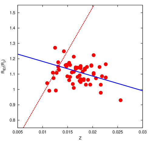
Figure 12: Planetary radius $R_{l\rm Et}$ (equation 25) with respect to $Z$. The planets with very large radii are excluded. The only planets with $R_{\rm p}<1.45{R}_{\rm J}~{}$ are considered. We subtract the effects of irradiation energy ($l_{-}$) and tidal interaction, and add the cooling effect to the observed $R_{\rm p}$. The resultant radius $R_{l\rm Et}$ is plotted with respect to $Z$. For the large part of the $Z$ range there is an anti-correlation between $R_{l\rm Et}$ and $Z$. For low $Z$, however, the relation between $R_{l\rm Et}$ and $Z$ is likely linear. The dashed and solid lines are for the ranges $Z<0.014$ and $Z>0.014$, respectively.

Radius of a planet depends on many parameters. These are irradiation energy ($l_{-}$), the tidal energy and the cooling rates. There are some studies in the literature in which relation between planetary radius and stellar metallicity is examined (see, e.g. Guillot et al. (2006) and Miller & Fortney (2011)). An inverse relation is found in these studies. Such a relation is very important for interior models of the planets. We want to check if there is a relation for the majority of the up-to-date planetary data.

Effect of any parameter on the planetary radii can be subtracted from $R_{\rm p}$. For $l_{-}$, for example, which is the most effective mechanism on $R_{\rm p}$,

$$R_{l}=R_{\rm p}-\frac{\Delta R_{\rm p}}{\Delta\log(l_{-})}\delta\log(l_{-}).$$ (23)

$R_{l}$ is the planetary radius if $l_{-}=0$. After subtracting the effect of $l_{-}$, we find relation between $R_{l}$ and $\log(\dot{E})$. Then, the effect of $\log(\dot{E})$ is also subtracted:

$$R_{l\rm E}=R_{l}-\frac{\Delta R_{l}}{\Delta\log(\dot{E})}\delta\log(\dot{E}).$$ (24)

For the effect of cooling,

$$R_{l\rm Et}=R_{l\rm E}+\frac{\Delta R_{l\rm E}}{\Delta t_{9}}\delta t_{9}.$$ (25)

$R_{l\rm Et}$ is the initial planetary radius if there were no irradiation energy and tidal interaction. In Fig. 12, $R_{l\rm Et}$ is plotted with respect to stellar metallicity $Z$. We note that metallicity influences the planetary radius. For $Z>0.014$, the slope is negative and found as $-9.5\pm 3.4$. This result is in very good agreement with the findings of Guillot et al. (2006) and Miller & Fortney (2011). For $Z<0.014$, however, there is a very sharp positive slope for this narrow range. Thus, metallicity works on planetary radius in two opposite ways. The maximum radius occurs about $Z\approx 0.014$–$0.015$.

For our understanding of the relation between metallicity and planet radius, two key parameters are very important. They are mass of the metal core and opacity in the envelope. The metallicity is a very strong source of opacity. As metallicity increases, planet size does not rapidly decrease because energy escape becomes difficult. This is the case for low-$Z$ range. The higher the metallicity is, the greater the radius is. For the high metallicity regime, it is expected that mass of the metal core increases as metallicity increases. The higher the metal core mass is, the smaller the radius is. However, for this regime, the alternative explanation may be based on the high binding energies of heavy elements. In the formation of planets, the majority of molecules is transformed into ionized gas, at least in the core regions. Some part of the heat gained from contraction is used for this transformation. If metallicity is very high then more energy is used to ionize matter and therefore the interior of planets with high $Z$ becomes cooler than that of planets with low $Z$. The cooler the interior is, the smaller the radius is.

4.6 Variation of planetary mass in time and possible effect of evaporation

To decipher detailed effects of irradiation on fundamental and orbital parameters of planets is a very difficult job. In addition to variation of planetary radius due to irradiation and time, planetary mass may also change depending on the amount of energy the planets expose.

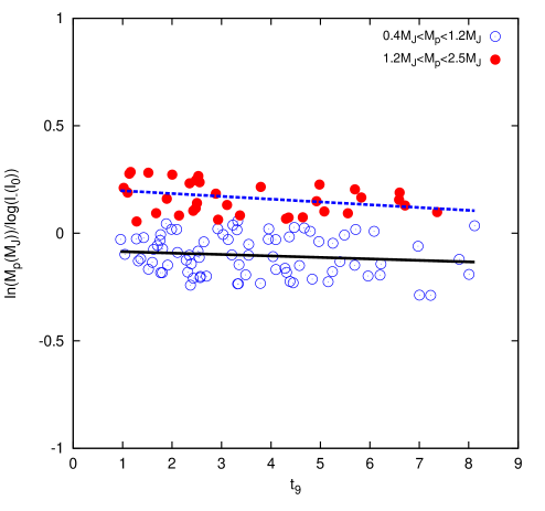
Figure 13: Planetary mass divided by $\log(l_{-})$ with respect to age ($t_{9}$). The solid and dashed lines are the fitted lines for the mass ranges $0.4{M}_{\rm J}~{}<M_{\rm p}<1.2{M}_{\rm J}~{}$ (circle) and $1.2{M}_{\rm J}~{}<M_{\rm p}<2.5{M}_{\rm J}~{}$ (filled circle), respectively.

Planetary mass $\ln(M_{\rm p})$ divided by $\log(l_{-})$ is plotted with respect to $t_{9}=t/(10^{9}$ Gyr$)$ in Fig. 13. We note that there is a small, but not negligible, time variation of $\ln(M_{\rm p})/\log(l_{-})$. We also note that the slope for the young systems is higher than that for the old systems. This is in agreement with the findings of Valencia et al. (2010) and Lopez, Fortney & Miller (2012). From the slope over all range of age, we can write

$$\frac{\Delta(\ln(M_{\rm p})/\log(l_{-}))}{\Delta t_{9}}=-{(0.0130\pm 0.0064)}.$$ (26)

If we assume that time variation of $l_{-}$ is negligibly small, we find

$$\dot{M_{\rm p}}=\frac{\Delta\ln(M_{\rm p})}{\Delta t_{9}}=-{(0.0130\pm 0.0064)}\log(l_{-}).$$ (27)

for $1.2{M}_{\rm J}~{}<M_{\rm p}<2.5{M}_{\rm J}~{}$. This variation of planetary mass may be a result of evaporation. Equation (27) gives mass-loss rate for these giant gas planets as $10^{11}-10^{13}$ g s^-1. The slope in Fig. 13 for the lower planetary mass range ($0.4{M}_{\rm J}~{}<M_{\rm p}<1.2{M}_{\rm J}~{}$), however, is $0.0068\pm 0.0058$. It is significantly less than 0.013. Then, for the low-mass giant gas planets ($M_{\rm p}<1.2{M}_{\rm J}~{}$)

$$\dot{M_{\rm p}}=\frac{\Delta\ln(M_{\rm p})}{\Delta t_{9}}=-{(0.0068\pm 0.0058)}\log(l_{-}).$$ (28)

This gives mass-loss rates of the giants gas planets as $10^{10}$–$10^{12}$ g s^-1.

There are several studies in the literature devoted to present behaviour of the planetary mass-loss rates (see, e.g Valencia et al. 2010 and Lopez, Fortney & Miller 2012). Linsky et al. (2010) find mass-loss rate for HD209458 b as $(0.8$–$4)10^{11}$ g s^-1. Using its age and $\log(l_{-})$, given in the online Table A1, the mass-loss rate is found as $\dot{M_{\rm p}}=(1$–$18)10^{11}$ g s^-1 from equation (28). Although its uncertainty is high, the lower part of its range is in agreement with the observed rate.

4.7 Initial planetary mass

If evaporation of planets really occurs, we can estimate the initial masses ($M_{\rm pi}$) of the giant gas planets by using equation (27) and (28): for $1.2{M}_{\rm J}~{}<M_{\rm p}<2.5{M}_{\rm J}~{}$,

$$M_{\rm pi}=M_{\rm p}{\rm e}^{{(0.0130\pm 0.0064)}\log(l_{-})t_{9}};$$ (29)

for $0.4{M}_{\rm J}~{}<M_{\rm p}<1.2{M}_{\rm J}~{}$,

$$M_{\rm pi}=M_{\rm p}{\rm e}^{{(0.0068\pm 0.0058)}\log(l_{-})t_{9}}.$$ (30)

According to our findings, the mean value of the mass lost by the giant gas planets is about 12 per cent and the most irradiated planets lose 5 per cent of their mass in every 1 Gyr. The maximum amount of lost mass is about 33 per cent (HATS-2 b). These preliminary results need further investigation and must be tested.

5 Conclusion

There are many papers in the literature on the effect of the induced flux on the radius of planets. The main outcome of these studies is that the radius is greater in the systems with the high incident flux than in the systems with the low flux. The excess depends on the mass interval of the planet. We show that there is much more definite relation between radius and energy per gram per second ($l_{-}$), if $l_{-}$ is greater than $300-500$ $l_{0}$, where is irradiation energy per unit mass and time by a planet with 1 M_J and 1 R_J at 1 au in our Solar system. This mechanism is the most efficient one on planetary size. If $l_{-}$ is greater than 3000 $l_{0}$, then there is another relation. $T_{\rm eq}$ of these planets in this range is higher than 1500 K. The reason for this extra inflation may be due to dissociation of molecules. It is demonstrated in Fig. 10 that there are some giant planets, which have material in the atomic form in the heated region rather than molecular, and excess in radius. The maximum effect of molecular dissociation on radius is about 33 per cent.

Tidal interaction influences radius of giant gas planets if the orbit is eccentric. Using expression for energy rate given by Storch & Lai (2014), we show that this mechanism causes giant gas planets to expand up to 15 per cent and confirm that their Model 2 seems more realistic than Model 1.

We also develop new methods to determine metallicity and age of the host stars. If metallicity is computed from direct use of observed [Fe/H] values, $Z_{\rm Fe}$ ranges from 0.006 to 0.05. Regarding the facts that there is an inverse relation between [O/Fe] and [Fe/H] (Edvardsson et al. 1993) and oxygen is the most abundant heavy element, we also compute $Z_{\rm O}$ from [O/H] by using the observed relation between [O/H] and [Fe/H]. $Z_{\rm O}$ ranges from 0.009 to 0.026. The difference between $Z_{\rm O}$ and $Z_{\rm Fe}$ is very significant for high metallicity.

A new method is developed to compute age of the host stars. The method is based on their radius, mass and metallicity. It is relatively easy to apply. By using $Z_{\rm O}$, we find that age of the host stars ranges from 0.3 to 11.1 Gyr. The mean age is 4.2 Gyr. If we use $Z_{\rm Fe}$ as metallicity of the host stars, age is found as greater than the galactic age. This implies that $Z_{\rm O}$ is a better indicator for the total metallicity. Our method yields results in very good agreement with the ages from asteroseismic inferences (see Table 1).

We also present our preliminary results for time variation of planetary radius due to cooling and mass due to evaporation. The mass-loss is also a function of irradiation energy per gram per second. We find that highly irradiated gas planets ($\log(l_{-}/l_{0})>3.2$) loss about 5 per cent of their total mass in every 1 Gyr.

We also test if metallicity has any influence on planetary radius. We subtract the effects of irradiation energy, tidal energy rate and cooling on the radius. The resultant radius shows an inverse relation with stellar metallicity. For the low-metallicity regime, there are less data, but the situation is opposite of this.

Appendix A Online-only table for basic properties of the giant gas planets and their host stars

Table 3: Fundamental properties of the giant gas planets and their host stars. The data are taken from TEPCat. Columns are organized as name, mass, radius and effective temperature of the host stars, semi-major axis, period, eccentricity, planetary mass, radius, equilibrium temperature, incident flux, energy received per unit mass per unit time, and rate of energy dissipation due to tidal interaction. In the last two columns, age and metallicity computed from stellar properties are listed (see Section 3).

Planet	$M$	$R$	$T_{\rm eff}$	$a$	$P$	$e$	$M_{\rm p}$	$R_{\rm p}$	$T_{\rm eq}$	$F_{\rm I}$	$l_{-}$	$\log(\dot{E})$	age	$Z_{\rm O}$
	(M☉)	(R☉)	(K)	(AU)	(d)		(Mj)	(R${}_{\rm j})$	(K)	(${\rm F}_{\rm\oplus})$	($l_{0})$	(erg s-1)	(Gyr)
CoRoT-01 b	0.95	1.13	5950	0.0254	1.509	0.000	1.03	1.55	1915	2238$\pm$ 647	5227$\pm$ 938	—	6.7$\pm$ 3.2	0.011$\pm$ 0.003
CoRoT-02 b	1.00	0.90	5598	0.0283	1.743	0.014	3.57	1.46	1521	890$\pm$ 98	531$\pm$ 44	26.5$\pm$ 0.3	1.1$\pm$ 1.6	0.016$\pm$ 0.004
CoRoT-03 b	1.40	1.58	6740	0.0578	4.257	0.000	21.96	1.04	1695	1374$\pm$ 330	67$\pm$ 11	—	1.1$\pm$ 0.3	0.015$\pm$ 0.004
CoRoT-04 b	1.19	1.15	6190	0.0912	9.202	0.000	0.73	1.16	1058	208$\pm$ 47	384$\pm$ 113	—	1.1$\pm$ 0.6	0.016$\pm$ 0.004
CoRoT-05 b	1.02	1.05	6100	0.0500	4.038	0.090	0.47	1.18	1348	549$\pm$ 143	1635$\pm$ 480	25.5$\pm$ 0.8	3.3$\pm$ 2.1	0.011$\pm$ 0.003
CoRoT-06 b	1.05	1.04	6090	0.0855	8.887	0.000	2.96	1.18	1025	183$\pm$ 26	87$\pm$ 16	—	2.5$\pm$ 1.3	0.012$\pm$ 0.003
CoRoT-09 b	0.96	0.94	5613	0.4027	95.274	0.110	0.83	1.04	413	4$\pm$ 1	6$\pm$ 1	17.1$\pm$ 0.7	3.8$\pm$ 2.8	0.015$\pm$ 0.004
CoRoT-10 b	0.90	0.74	5075	0.1060	13.241	0.530	2.78	0.94	647	29$\pm$ 6	9$\pm$ 2	23.0$\pm$ 0.6	—	0.021$\pm$ 0.005
CoRoT-11 b	1.26	1.37	6440	0.0440	2.994	0.000	2.34	1.43	1735	1505$\pm$ 355	1308$\pm$ 322	—	2.0$\pm$ 1.1	0.015$\pm$ 0.004
CoRoT-12 b	1.02	1.05	5675	0.0394	2.828	0.000	0.89	1.35	1410	656$\pm$ 127	1348$\pm$ 268	—	5.0$\pm$ 2.7	0.018$\pm$ 0.005
CoRoT-13 b	1.09	1.27	5945	0.0510	4.035	0.000	1.31	1.25	1432	699$\pm$ 163	836$\pm$ 162	—	5.6$\pm$ 1.6	0.015$\pm$ 0.004
CoRoT-14 b	1.13	1.19	6035	0.0269	1.512	0.000	7.67	1.02	1936	2335$\pm$ 840	315$\pm$ 69	—	3.4$\pm$ 1.6	0.016$\pm$ 0.004
CoRoT-15 b	1.31	1.36	6350	0.0458	3.060	0.000	64.90	1.04	1670	1287$\pm$ 1001	21$\pm$ 15	—	1.3$\pm$ 1.0	0.017$\pm$ 0.004
CoRoT-16 b	1.10	1.19	5650	0.0618	5.352	0.330	0.54	1.17	–	339$\pm$ 120	867$\pm$ 374	26.1$\pm$ 1.0	4.8$\pm$ 1.7	0.019$\pm$ 0.005
CoRoT-17 b	1.04	1.62	5740	0.0481	3.768	0.000	2.46	1.01	1610	1105$\pm$ 754	455$\pm$ 359	—	7.4$\pm$ 1.8	0.015$\pm$ 0.004
CoRoT-18 b	0.86	0.92	5440	0.0286	1.900	0.000	3.27	1.25	1490	820$\pm$ 200	392$\pm$ 72	—	7.5$\pm$ 3.7	0.014$\pm$ 0.003
CoRoT-19 b	1.18	1.58	6090	0.0512	3.897	0.000	1.09	1.19	1630	1170$\pm$ 661	1520$\pm$ 793	—	4.5$\pm$ 1.4	0.015$\pm$ 0.004
CoRoT-20 b	1.11	1.34	5880	0.0892	9.243	0.000	5.06	1.16	1100	242$\pm$ 163	64$\pm$ 33	—	6.2$\pm$ 1.8	0.018$\pm$ 0.005
CoRoT-21 b	1.39	1.95	6200	0.0417	2.725	0.000	2.26	1.27	–	2901$\pm$ 965	2070$\pm$ 758	—	2.5$\pm$ 0.4	0.015$\pm$ 0.004
CoRoT-23 b	1.12	1.74	5900	0.0481	3.631	0.160	3.06	1.18	1710	1424$\pm$ 598	648$\pm$ 276	26.3$\pm$ 1.1	5.7$\pm$ 1.5	0.016$\pm$ 0.004
CoRoT-26 b	1.09	1.79	5590	0.0526	4.205	0.000	0.52	1.26	1600	1015$\pm$ 315	3099$\pm$ 937	—	6.3$\pm$ 1.2	0.015$\pm$ 0.004
HAT-P-01 b	1.15	1.17	5975	0.0556	4.465	0.000	0.52	1.32	1322	510$\pm$ 54	1690$\pm$ 109	—	2.7$\pm$ 0.3	0.018$\pm$ 0.004
HAT-P-02 b	1.28	1.68	6290	0.0674	5.633	0.508a	8.74	1.19	1516	873$\pm$ 210	141$\pm$ 32	26.3$\pm$ 0.6	3.7$\pm$ 0.4	0.018$\pm$ 0.005
HAT-P-03 b	0.90	0.87	5185	0.0384	2.900	0.000	0.58	0.95	1189	332$\pm$ 42	510$\pm$ 55	—	6.0$\pm$ 3.6	0.021$\pm$ 0.005
HAT-P-04 b	1.27	1.60	5860	0.0446	3.057	0.004a	0.68	1.34	1691	1359$\pm$ 356	3573$\pm$ 663	23.7$\pm$ 0.7	4.0$\pm$ 1.1	0.020$\pm$ 0.005
HAT-P-05 b	1.16	1.14	5960	0.0408	2.788	0.000	1.06	1.25	1517	880$\pm$ 144	1301$\pm$ 224	—	2.0$\pm$ 1.1	0.020$\pm$ 0.005
HAT-P-06 b	1.29	1.52	6570	0.0524	3.853	0.023a	1.06	1.39	1704	1401$\pm$ 248	2566$\pm$ 435	24.7$\pm$ 0.5	2.1$\pm$ 0.5	0.013$\pm$ 0.003
HAT-P-07 b	1.51	1.96	6350	0.0380	2.205	0.005a	1.80	1.47	2194	3853$\pm$ 345	4597$\pm$ 202	25.1$\pm$ 0.2	1.9$\pm$ 0.1	0.021$\pm$ 0.005
HAT-P-08 b	1.19	1.48	6200	0.0439	3.076	0.003a	1.27	1.32	1713	1497$\pm$ 208	2049$\pm$ 209	23.4$\pm$ 0.4	4.4$\pm$ 0.9	0.015$\pm$ 0.004
HAT-P-09 b	1.28	1.34	6350	0.0529	3.923	0.000	0.78	1.38	1540	935$\pm$ 249	2289$\pm$ 575	—	1.6$\pm$ 0.8	0.018$\pm$ 0.004
HAT-P-13 b	1.32	1.76	5653	0.0438	2.916	0.013a	0.91	1.49	1725	1471$\pm$ 216	3591$\pm$ 316	25.1$\pm$ 0.3	3.9$\pm$ 0.6	0.024$\pm$ 0.006
HAT-P-14 b	1.42	1.59	6600	0.0611	4.628	0.115a	2.27	1.22	1624	1155$\pm$ 173	756$\pm$ 100	25.4$\pm$ 0.4	1.2$\pm$ 0.3	0.017$\pm$ 0.004
HAT-P-15 b	1.01	1.08	5568	0.0964	10.864	0.208a	1.95	1.07	904	108$\pm$ 17	63$\pm$ 7	23.5$\pm$ 0.4	6.4$\pm$ 1.5	0.020$\pm$ 0.005
HAT-P-16 b	1.22	1.16	6140	0.0413	2.776	0.042a	4.19	1.19	1567	1003$\pm$ 120	338$\pm$ 31	25.8$\pm$ 0.3	0.8$\pm$ 0.7	0.018$\pm$ 0.004
HAT-P-17 b	0.86	0.84	5246	0.0882	10.339	0.342a	0.53	1.01	792	61$\pm$ 8	117$\pm$ 10	24.1$\pm$ 0.3	5.3$\pm$ 2.8	0.015$\pm$ 0.004
HAT-P-20 b	0.76	0.69	4595	0.0361	2.876	0.016a	7.25	0.87	970	147$\pm$ 23	15$\pm$ 1	24.1$\pm$ 0.3	5.6$\pm$ 4.9	0.023$\pm$ 0.006
HAT-P-21 b	0.95	1.11	5588	0.0494	4.124	0.228	4.06	1.02	1283	438$\pm$ 103	113$\pm$ 24	26.0$\pm$ 0.6	8.4$\pm$ 1.8	0.015$\pm$ 0.004
HAT-P-22 b	0.92	1.04	5302	0.0414	3.212	0.006a	2.15	1.08	1283	447$\pm$ 75	243$\pm$ 33	23.5$\pm$ 0.4	11.1$\pm$ 2.1	0.020$\pm$ 0.005
HAT-P-23 b	1.13	1.20	5905	0.0232	1.213	0.106	2.09	1.37	2056	2935$\pm$ 570	2628$\pm$ 485	29.1$\pm$ 0.4	3.8$\pm$ 0.7	0.018$\pm$ 0.005
HAT-P-24 b	1.19	1.29	6373	0.0464	3.355	0.033a	0.68	1.24	1624	1151$\pm$ 210	2612$\pm$ 421	25.2$\pm$ 0.4	2.6$\pm$ 0.5	0.013$\pm$ 0.003
HAT-P-25 b	1.01	0.96	5500	0.0466	3.653	0.032	0.57	1.19	1202	347$\pm$ 66	868$\pm$ 151	24.8$\pm$ 0.5	3.5$\pm$ 1.2	0.022$\pm$ 0.005
HAT-P-27 b	0.94	0.90	5316	0.0403	3.040	0.078	0.66	1.04	1207	356$\pm$ 66	581$\pm$ 115	25.8$\pm$ 0.5	4.6$\pm$ 1.9	0.022$\pm$ 0.005
HAT-P-28 b	1.02	1.10	5680	0.0434	3.257	0.051	0.63	1.21	1384	603$\pm$ 157	1416$\pm$ 347	25.6$\pm$ 0.7	5.7$\pm$ 1.4	0.018$\pm$ 0.004
HAT-P-29 b	1.21	1.22	6087	0.0667	5.723	0.061a	0.78	1.11	1260	415$\pm$ 124	653$\pm$ 224	24.1$\pm$ 0.8	2.1$\pm$ 0.6	0.020$\pm$ 0.005
HAT-P-30 b	1.24	1.22	6338	0.0419	2.811	0.020a	0.71	1.34	1630	1218$\pm$ 163	3076$\pm$ 419	25.4$\pm$ 0.4	1.0$\pm$ 0.5	0.018$\pm$ 0.004
HAT-P-31 b	1.22	1.36	6065	0.0550	5.005	0.242a	2.17	1.07	1450	742$\pm$ 749	391$\pm$ 194	25.9$\pm$ 2.9	3.2$\pm$ 1.0	0.018$\pm$ 0.005
HAT-P-32 b	1.16	1.22	6207	0.0343	2.150	0.200a	0.86	1.79	1786	1683$\pm$ 178	6264$\pm$ 1369	28.8$\pm$ 0.2	2.6$\pm$ 0.6	0.015$\pm$ 0.004
HAT-P-33 b	1.38	1.64	6446	0.0499	3.475	0.130a	0.76	1.69	1782	1668$\pm$ 193	6223$\pm$ 1157	27.0$\pm$ 0.3	1.8$\pm$ 0.2	0.017$\pm$ 0.004
HAT-P-34 b	1.39	1.53	6442	0.0677	5.453	0.411a	3.33	1.20	1520	794$\pm$ 202	342$\pm$ 94	26.4$\pm$ 0.7	1.4$\pm$ 0.3	0.020$\pm$ 0.005
HAT-P-35 b	1.24	1.43	6178	0.0498	3.647	0.025	1.05	1.33	1581	1085$\pm$ 184	1828$\pm$ 326	24.9$\pm$ 0.5	3.3$\pm$ 0.5	0.018$\pm$ 0.004
HAT-P-36 b	1.02	1.10	5560	0.0238	1.327	0.063	1.83	1.26	1823	1819$\pm$ 377	1586$\pm$ 263	28.2$\pm$ 0.5	6.6$\pm$ 1.7	0.021$\pm$ 0.005
HAT-P-37 b	0.93	0.88	5500	0.0379	2.797	0.058	1.17	1.18	1271	439$\pm$ 105	522$\pm$ 114	26.0$\pm$ 0.5	3.3$\pm$ 2.1	0.016$\pm$ 0.004
HAT-P-39 b	1.40	1.63	6340	0.0509	3.544	0.000	0.60	1.57	1752	1478$\pm$ 275	6091$\pm$ 1844	—	1.6$\pm$ 0.3	0.019$\pm$ 0.005
HAT-P-40 b	1.51	2.21	6080	0.0608	4.457	0.000	0.62	1.73	1770	1615$\pm$ 227	7860$\pm$ 1049	—	2.3$\pm$ 0.2	0.020$\pm$ 0.005
HAT-P-41 b	1.42	1.68	6390	0.0426	2.694	0.000	0.80	1.68	1941	2336$\pm$ 362	8291$\pm$ 1805	—	1.7$\pm$ 0.3	0.020$\pm$ 0.005
HAT-P-42 b	1.18	1.53	5743	0.0575	4.642	0.000	0.98	1.28	1427	689$\pm$ 173	1153$\pm$ 418	—	5.5$\pm$ 1.0	0.021$\pm$ 0.005
HAT-P-43 b	1.05	1.10	5645	0.0443	3.333	0.000	0.66	1.28	1361	566$\pm$ 76	1412$\pm$ 303	—	5.4$\pm$ 0.9	0.020$\pm$ 0.005
HAT-P-45 b	1.26	1.32	6330	0.0452	3.129	0.049	0.89	1.43	1652	1227$\pm$ 404	2798$\pm$ 1116	26.0$\pm$ 0.8	1.8$\pm$ 0.6	0.017$\pm$ 0.004
HAT-P-46 b	1.28	1.40	6120	0.0577	4.463	0.123	0.49	1.28	1458	737$\pm$ 393	2465$\pm$ 1450	25.7$\pm$ 1.3	2.4$\pm$ 0.9	0.022$\pm$ 0.005
HATS-1 b	0.99	1.04	5870	0.0444	3.446	0.120	1.86	1.30	1359	582$\pm$ 204	532$\pm$ 207	26.4$\pm$ 0.8	5.0$\pm$ 1.7	0.014$\pm$ 0.004
HATS-2 b	0.88	0.90	5227	0.0230	1.354	0.000	1.35	1.17	1577	1021$\pm$ 144	1036$\pm$ 168	—	7.4$\pm$ 2.5	0.018$\pm$ 0.005
HATS-3 b	1.21	1.40	6351	0.0485	3.548	0.000	1.07	1.38	1648	1224$\pm$ 131	2179$\pm$ 387	—	2.9$\pm$ 0.4	0.013$\pm$ 0.003
HD017156 b	1.30	1.49	6079	0.1637	21.216	0.675	3.26	1.07	883	101$\pm$ 13	35$\pm$ 3	—	2.7$\pm$ 0.6	0.020$\pm$ 0.005
HD080606 b	1.02	1.04	5574	0.4564	111.437	0.933	4.11	1.00	405	4$\pm$ 0	1$\pm$ 0	—	5.8$\pm$ 2.0	0.023$\pm$ 0.006
HD189733 b	0.84	0.75	5050	0.0314	2.219	0.004	1.15	1.15	1191	334$\pm$ 46	385$\pm$ 38	24.3$\pm$ 0.4	1.6$\pm$ 3.2	0.015$\pm$ 0.004
HD209458 b	1.15	1.16	6117	0.0475	3.525	0.000	0.71	1.38	1459	753$\pm$ 60	2008$\pm$ 97	—	2.3$\pm$ 0.6	0.016$\pm$ 0.004
KELT-1 b	1.34	1.47	6516	0.0247	1.218	0.010	27.38	1.12	2423	5731$\pm$ 703	260$\pm$ 26	26.5$\pm$ 0.4	1.5$\pm$ 0.4	0.016$\pm$ 0.004
KELT-2 b	1.31	1.84	6151	0.0550	4.114	0.000	1.52	1.29	1712	1430$\pm$ 192	1561$\pm$ 245	—	3.1$\pm$ 0.5	0.016$\pm$ 0.004
KELT-3 b	1.28	1.47	6306	0.0412	2.703	0.000	1.48	1.35	1811	1810$\pm$ 275	2217$\pm$ 336	—	2.5$\pm$ 0.5	0.016$\pm$ 0.004
KELT-6 b	1.09	1.58	6102	0.0794	7.846	0.220	0.43	1.19	1313	493$\pm$ 126	1631$\pm$ 526	24.6$\pm$ 0.7	5.2$\pm$ 0.7	0.011$\pm$ 0.003
Kepler-05 b	1.30	1.54	6297	0.0497	3.548	0.000	2.03	1.21	1692	1364$\pm$ 177	980$\pm$ 80	—	2.6$\pm$ 0.3	0.016$\pm$ 0.004
Kepler-06 b	1.11	1.26	5647	0.0444	3.235	0.000	0.63	1.17	1451	737$\pm$ 162	1591$\pm$ 305	—	6.2$\pm$ 2.9	0.023$\pm$ 0.006
Kepler-07 b	1.41	2.03	5933	0.0632	4.885	0.000	0.45	1.65	1619	1144$\pm$ 117	6867$\pm$ 1347	—	2.6$\pm$ 0.5	0.017$\pm$ 0.004
Kepler-08 b	1.23	1.50	6213	0.0485	3.523	0.000	0.59	1.38	1662	1271$\pm$ 248	4108$\pm$ 1055	—	3.4$\pm$ 0.7	0.014$\pm$ 0.004
Kepler-12 b	1.16	1.49	5947	0.0555	4.438	0.000	0.43	1.71	1485	809$\pm$ 184	5478$\pm$ 1118	—	5.2$\pm$ 1.9	0.017$\pm$ 0.004
Kepler-14 b	1.32	2.09	6395	0.0771	6.790	0.040	7.68	1.13	1605	1103$\pm$ 189	182$\pm$ 24	23.3$\pm$ 0.4	3.3$\pm$ 0.5	0.018$\pm$ 0.004
Kepler-15 b	1.08	1.25	5595	0.0583	4.943	0.000	0.70	1.29	1251	406$\pm$ 100	970$\pm$ 219	—	7.8$\pm$ 3.0	0.023$\pm$ 0.006
Kepler-17 b	1.07	0.98	5781	0.0260	1.486	0.000	2.34	1.31	1712	1427$\pm$ 184	1047$\pm$ 78	—	1.5$\pm$ 1.4	0.021$\pm$ 0.005
Kepler-30 c	0.99	0.95	5498	0.3000	60.323	0.011	2.01	1.10	–	8$\pm$ -52	4$\pm$ 0	16.4$\pm$ -19.7	3.6$\pm$ 2.8	0.019$\pm$ 0.005
Kepler-39 b	1.08	1.23	6260	0.1539	21.087	0.121	17.90	1.09	851	87$\pm$ 29	5$\pm$ 1	21.2$\pm$ 0.9	4.0$\pm$ 2.2	0.011$\pm$ 0.003
Kepler-40 b	1.46	2.48	6510	0.0802	6.873	0.000	2.16	1.44	1744	1541$\pm$ 504	1480$\pm$ 541	—	2.3$\pm$ 0.6	0.017$\pm$ 0.004
Kepler-41 b	0.94	0.94	5660	0.0290	1.856	0.000	0.49	0.85	1554	969$\pm$ 258	1427$\pm$ 446	—	4.4$\pm$ 3.4	0.014$\pm$ 0.003
Kepler-43 b	1.24	1.33	6041	0.0440	3.024	0.000	3.09	1.12	1603	1095$\pm$ 244	440$\pm$ 62	—	2.9$\pm$ 1.2	0.022$\pm$ 0.006
Kepler-44 b	1.21	1.46	5757	0.0457	3.247	0.000	1.03	1.20	1568	1006$\pm$ 334	1407$\pm$ 376	—	4.8$\pm$ 1.5	0.021$\pm$ 0.005
Kepler-56 c	1.32	4.23	4840	0.1652	21.402	-1.000	0.57	0.87	–	323$\pm$ 71	433$\pm$ 90	—	3.4$\pm$ 0.9	0.019$\pm$ 0.005
Kepler-74 b	1.40	1.51	6050	0.0840	7.341	0.287	0.68	1.32	1250	388$\pm$ 229	995$\pm$ 342	25.3$\pm$ 1.7	1.3$\pm$ 0.7	0.023$\pm$ 0.006
Kepler-75 b	0.88	0.88	5330	0.0800	8.885	0.569	9.90	1.03	850	87$\pm$ 26	9$\pm$ 1	—	5.3$\pm$ 3.4	0.014$\pm$ 0.004
Kepler-77 b	0.95	0.99	5520	0.0450	3.579	0.000	0.43	0.96	1440	403$\pm$ 45	864$\pm$ 93	—	7.0$\pm$ 1.9	0.019$\pm$ 0.005
Kepler-87 b	1.10	1.82	5600	0.4810	114.736	0.036	1.02	1.20	478	12$\pm$ 2	17$\pm$ 1	15.9$\pm$ 0.6	5.3$\pm$ 0.9	0.012$\pm$ 0.003
Kepler-91 b	1.31	6.20	4550	0.0720	6.247	0.066	0.88	1.38	–	2853$\pm$ 493	6210$\pm$ 1298	24.4$\pm$ 0.4	3.3$\pm$ 0.7	0.017$\pm$ 0.004
KOI-205 b	0.93	0.84	5237	0.0987	11.720	0.000	39.90	0.81	737	49$\pm$ 5	0$\pm$ 0	—	2.2$\pm$ 1.8	0.018$\pm$ 0.005
KOI-415 b	0.94	1.25	5810	0.5930	166.788	0.698	62.14	0.79	–	4$\pm$ 0	0$\pm$ 0	—	9.3$\pm$ 2.1	0.011$\pm$ 0.003
OGLE-TR-010 b	1.28	1.52	6075	0.0452	3.101	0.000	0.68	1.72	1702	1385$\pm$ 322	6027$\pm$ 2100	—	3.5$\pm$ 0.8	0.021$\pm$ 0.005
OGLE-TR-056 b	1.34	1.74	6119	0.0245	1.212	0.000	1.41	1.73	2482	6311$\pm$ 896	13458$\pm$ 2522	—	3.4$\pm$ 0.7	0.020$\pm$ 0.005
OGLE-TR-111 b	0.85	0.82	5044	0.0468	4.014	0.000	0.55	1.01	1019	179$\pm$ 31	333$\pm$ 85	—	6.6$\pm$ 5.3	0.019$\pm$ 0.005
OGLE-TR-113 b	0.75	0.77	4790	0.0226	1.432	0.000	1.23	1.09	1342	540$\pm$ 135	520$\pm$ 136	—	9.7$\pm$ 11.7	0.017$\pm$ 0.004
OGLE-TR-132 b	1.29	1.34	6210	0.0303	1.690	0.000	1.17	1.23	1991	2610$\pm$ 571	3370$\pm$ 843	—	1.9$\pm$ 1.1	0.023$\pm$ 0.006
OGLE-TR-182 b	1.19	1.53	5924	0.0520	3.979	0.000	1.06	1.47	1550	955$\pm$ 277	1947$\pm$ 646	—	5.7$\pm$ 0.7	0.023$\pm$ 0.006
OGLE-TR-211 b	1.31	1.56	6325	0.0510	3.677	0.000	0.75	1.26	1686	1341$\pm$ 426	2849$\pm$ 1283	—	2.5$\pm$ 0.5	0.017$\pm$ 0.004
OGLE-TR-L9 b	1.43	1.50	6933	0.0405	2.486	0.000	4.40	1.63	2034	2845$\pm$ 393	1724$\pm$ 684	—	0.5$\pm$ 0.4	0.014$\pm$ 0.004
Qatar-1 1b	0.85	0.80	4910	0.0234	1.420	0.000	1.33	1.18	1389	608$\pm$ 131	636$\pm$ 120	—	5.1$\pm$ 2.6	0.019$\pm$ 0.005
TrES-1 b	0.89	0.82	5226	0.0395	3.030	0.000	0.76	1.10	1147	287$\pm$ 36	456$\pm$ 59	—	2.7$\pm$ 2.9	0.016$\pm$ 0.004
TrES-2 b	0.99	0.96	5850	0.0357	2.471	0.004a	1.21	1.19	1466	768$\pm$ 83	906$\pm$ 71	23.9$\pm$ 0.3	2.9$\pm$ 1.7	0.013$\pm$ 0.003
TrES-3 b	0.92	0.82	5650	0.0228	1.306	0.170a	1.90	1.31	1638	1197$\pm$ 112	1082$\pm$ 66	29.2$\pm$ 0.2	1.0$\pm$ 0.9	0.012$\pm$ 0.003
TrES-4 b	1.34	1.83	6200	0.0502	3.554	0.015a	0.90	1.74	1805	1770$\pm$ 324	5942$\pm$ 989	25.1$\pm$ 0.5	3.1$\pm$ 0.6	0.018$\pm$ 0.005
TrES-5 b	0.89	0.87	5171	0.0245	1.482	0.000	1.78	1.21	1484	804$\pm$ 91	661$\pm$ 46	—	5.7$\pm$ 1.7	0.019$\pm$ 0.005
WASP-01 b	1.26	1.47	6213	0.0392	2.520	0.008a	0.98	1.49	1830	1868$\pm$ 243	4250$\pm$ 551	25.1$\pm$ 0.4	3.0$\pm$ 0.6	0.019$\pm$ 0.005
WASP-02 b	0.85	0.82	5170	0.0309	2.152	0.005a	0.88	1.06	1286	454$\pm$ 58	583$\pm$ 55	24.4$\pm$ 0.4	5.3$\pm$ 3.6	0.016$\pm$ 0.004
WASP-03 b	1.11	1.30	6340	0.0305	1.847	0.007a	1.77	1.35	2020	2627$\pm$ 501	2689$\pm$ 418	25.5$\pm$ 0.5	5.8$\pm$ 1.6	0.018$\pm$ 0.005
WASP-04 b	0.93	0.91	5540	0.0232	1.338	0.003a	1.25	1.36	1673	1303$\pm$ 155	1941$\pm$ 160	25.8$\pm$ 0.3	4.3$\pm$ 2.5	0.015$\pm$ 0.004
WASP-05 b	1.03	1.09	5770	0.0274	1.628	0.000	1.60	1.17	1753	1569$\pm$ 236	1358$\pm$ 171	—	4.9$\pm$ 1.4	0.017$\pm$ 0.004
WASP-06 b	0.88	0.87	5375	0.0421	3.361	0.054	0.50	1.22	1194	320$\pm$ 46	953$\pm$ 115	25.6$\pm$ 0.4	4.4$\pm$ 2.6	0.012$\pm$ 0.003
WASP-07 b	1.32	1.48	6520	0.0624	4.955	0.034a	0.98	1.37	1530	910$\pm$ 179	1753$\pm$ 472	24.4$\pm$ 0.6	1.8$\pm$ 0.5	0.015$\pm$ 0.004
WASP-08 b	1.03	0.94	5600	0.0801	8.159	0.304a	2.25	1.04	–	122$\pm$ 24	58$\pm$ 2	24.6$\pm$ 0.2	1.6$\pm$ 1.6	0.019$\pm$ 0.005
WASP-11 b	0.83	0.79	4980	0.0435	3.722	0.000	0.46	1.00	1020	182$\pm$ 23	399$\pm$ 49	—	5.5$\pm$ 2.8	0.018$\pm$ 0.004
WASP-12 b	1.36	1.60	6313	0.0231	1.091	0.037a	1.42	1.85	2578	6864$\pm$ 1137	16544$\pm$ 1503	29.0$\pm$ 0.5	2.1$\pm$ 0.4	0.020$\pm$ 0.005
WASP-13 b	1.22	1.66	6025	0.0557	4.353	0.000	0.51	1.53	1531	1047$\pm$ 182	4774$\pm$ 1084	—	4.3$\pm$ 1.3	0.017$\pm$ 0.004
WASP-14 b	1.35	1.67	6462	0.0372	2.243	0.082a	7.90	1.63	2090	3139$\pm$ 697	1059$\pm$ 180	27.6$\pm$ 0.6	2.1$\pm$ 0.6	0.015$\pm$ 0.004
WASP-15 b	1.30	1.52	6573	0.0516	3.752	0.038a	0.59	1.41	1676	1455$\pm$ 183	4873$\pm$ 474	25.3$\pm$ 0.3	2.4$\pm$ 0.4	0.017$\pm$ 0.004
WASP-16 b	0.98	1.09	5630	0.0415	3.119	0.015a	0.83	1.22	1389	618$\pm$ 101	1103$\pm$ 122	24.6$\pm$ 0.4	7.0$\pm$ 2.0	0.017$\pm$ 0.004
WASP-17 b	1.29	1.58	6550	0.0514	3.735	0.039a	0.48	1.93	1755	1570$\pm$ 240	12289$\pm$ 1524	26.0$\pm$ 0.4	2.3$\pm$ 0.5	0.011$\pm$ 0.003
WASP-18 b	1.29	1.25	6400	0.0205	0.941	0.007a	10.52	1.20	2411	5617$\pm$ 665	774$\pm$ 59	27.0$\pm$ 0.3	0.5$\pm$ 0.5	0.017$\pm$ 0.004
WASP-19 b	0.94	1.02	5460	0.0163	0.789	0.002a	1.14	1.41	2077	3097$\pm$ 386	5405$\pm$ 331	26.9$\pm$ 0.3	8.1$\pm$ 2.1	0.018$\pm$ 0.005
WASP-22 b	1.11	1.22	6020	0.0470	3.533	0.011a	0.59	1.16	1466	793$\pm$ 106	1810$\pm$ 243	23.9$\pm$ 0.4	4.3$\pm$ 0.5	0.016$\pm$ 0.004
WASP-23 b	0.84	0.82	5046	0.0380	2.944	0.000	0.92	1.07	1152	270$\pm$ 53	336$\pm$ 42	—	5.7$\pm$ 4.0	0.016$\pm$ 0.004
WASP-24 b	1.15	1.35	6297	0.0362	2.341	0.003a	1.09	1.38	1781	1975$\pm$ 195	3464$\pm$ 274	26.3$\pm$ 0.2	4.7$\pm$ 0.4	0.017$\pm$ 0.004
WASP-25 b	1.00	0.92	5736	0.0473	3.765	0.000	0.58	1.22	1212	367$\pm$ 47	943$\pm$ 157	—	1.8$\pm$ 1.0	0.016$\pm$ 0.004
WASP-26 b	1.10	1.29	6034	0.0398	2.767	0.003	1.03	1.27	1623	1250$\pm$ 141	1957$\pm$ 253	23.6$\pm$ 0.4	6.1$\pm$ 0.7	0.018$\pm$ 0.005
WASP-30 b	1.25	1.39	6190	0.0553	4.157	0.000	62.50	0.95	1474	830$\pm$ 80	12$\pm$ 0	—	2.5$\pm$ 0.3	0.017$\pm$ 0.004
WASP-31 b	1.16	1.25	6175	0.0466	3.406	0.000	0.48	1.55	1575	942$\pm$ 106	4731$\pm$ 592	—	2.6$\pm$ 0.3	0.012$\pm$ 0.003
WASP-32 b	1.10	1.11	6100	0.0394	2.719	0.018	3.60	1.18	1560	986$\pm$ 168	381$\pm$ 52	25.1$\pm$ 0.4	2.5$\pm$ 0.6	0.013$\pm$ 0.003
WASP-33 b	1.56	1.51	7430	0.0259	1.220	0.000	3.27	1.68	2710	9288$\pm$ 877	8016$\pm$ 1963	—	0.3$\pm$ 0.1	0.017$\pm$ 0.004
WASP-34 b	1.01	0.93	5704	0.0524	4.318	0.011a	0.59	1.22	1250	299$\pm$ 87	755$\pm$ 148	23.5$\pm$ 0.6	1.8$\pm$ 2.1	0.017$\pm$ 0.004
WASP-35 b	1.07	1.09	6072	0.0432	3.162	0.000	0.72	1.32	1450	778$\pm$ 86	1882$\pm$ 299	—	3.2$\pm$ 0.7	0.014$\pm$ 0.004
WASP-36 b	1.04	0.95	5928	0.0264	1.537	0.000	2.30	1.28	1724	1435$\pm$ 139	1022$\pm$ 76	—	1.1$\pm$ 0.8	0.015$\pm$ 0.004
WASP-37 b	0.93	1.00	5940	0.0446	3.577	0.000	1.80	1.00	1323	565$\pm$ 128	315$\pm$ 63	—	5.1$\pm$ 3.6	0.009$\pm$ 0.002
WASP-38 b	1.20	1.33	6150	0.0752	6.872	0.033a	2.69	1.09	1292	402$\pm$ 46	178$\pm$ 13	23.0$\pm$ 0.3	2.6$\pm$ 0.4	0.013$\pm$ 0.003
WASP-41 b	0.94	0.91	5546	0.0403	3.052	0.000	0.92	1.21	1235	433$\pm$ 68	689$\pm$ 132	—	4.1$\pm$ 1.4	0.016$\pm$ 0.004
WASP-42 b	0.88	0.86	5315	0.0548	4.982	0.060	0.50	1.08	995	177$\pm$ 38	414$\pm$ 72	24.4$\pm$ 0.6	6.9$\pm$ 5.7	0.021$\pm$ 0.005
WASP-44 b	0.92	0.87	5400	0.0344	2.424	0.000	0.87	1.00	1304	481$\pm$ 127	556$\pm$ 93	—	3.6$\pm$ 4.2	0.016$\pm$ 0.004
WASP-45 b	0.91	0.94	5100	0.0405	3.126	0.000	1.01	1.16	1198	330$\pm$ 127	441$\pm$ 236	—	9.8$\pm$ 3.8	0.023$\pm$ 0.006
WASP-46 b	0.96	0.92	5600	0.0245	1.430	0.000	2.10	1.31	1654	1238$\pm$ 236	1011$\pm$ 113	—	2.5$\pm$ 1.1	0.010$\pm$ 0.002
WASP-47 b	1.08	1.15	5576	0.0520	4.159	0.000	1.14	1.15	1220	424$\pm$ 52	492$\pm$ 55	—	5.6$\pm$ 1.0	0.023$\pm$ 0.006
WASP-48 b	1.19	1.75	6000	0.0344	2.144	0.000	0.98	1.67	2030	3004$\pm$ 684	8549$\pm$ 1808	—	4.0$\pm$ 0.6	0.013$\pm$ 0.003
WASP-50 b	0.86	0.86	5518	0.0291	1.955	0.000	1.44	1.14	1410	717$\pm$ 85	646$\pm$ 60	—	6.7$\pm$ 4.1	0.018$\pm$ 0.004
WASP-52 b	0.87	0.79	5000	0.0272	1.750	0.000	0.46	1.27	1315	473$\pm$ 72	1659$\pm$ 150	—	2.4$\pm$ 2.1	0.016$\pm$ 0.004
WASP-54 b	1.21	1.83	6296	0.0499	3.694	0.067	0.64	1.65	1759	1895$\pm$ 270	8143$\pm$ 1206	26.2$\pm$ 0.4	4.1$\pm$ 0.4	0.015$\pm$ 0.004
WASP-55 b	1.01	1.06	6070	0.0533	4.466	0.000	0.57	1.30	1290	482$\pm$ 56	1429$\pm$ 210	—	5.2$\pm$ 1.3	0.017$\pm$ 0.004
WASP-56 b	1.02	1.11	5600	0.0546	4.167	0.000	0.57	1.09	1216	366$\pm$ 48	765$\pm$ 94	—	6.2$\pm$ 0.8	0.018$\pm$ 0.004
WASP-57 b	0.95	0.84	5600	0.0386	2.839	0.000	0.67	0.92	1251	414$\pm$ 107	517$\pm$ 56	—	—	0.011$\pm$ 0.003
WASP-58 b	0.94	1.17	5800	0.0561	5.017	0.000	0.89	1.37	1270	441$\pm$ 175	931$\pm$ 345	—	6.9$\pm$ 2.8	0.009$\pm$ 0.002
WASP-60 b	1.08	1.14	5900	0.0531	4.305	0.000	0.51	0.86	1320	501$\pm$ 159	721$\pm$ 248	—	3.8$\pm$ 0.8	0.015$\pm$ 0.004
WASP-61 b	1.22	1.36	6250	0.0514	3.856	0.000	2.06	1.24	1565	959$\pm$ 167	715$\pm$ 93	—	2.5$\pm$ 0.7	0.014$\pm$ 0.003
WASP-62 b	1.25	1.28	6230	0.0567	4.412	0.000	0.57	1.39	1440	689$\pm$ 106	2336$\pm$ 365	—	1.5$\pm$ 0.5	0.016$\pm$ 0.004
WASP-64 b	1.00	1.06	5550	0.0265	1.573	0.000	1.27	1.27	1689	1359$\pm$ 235	1728$\pm$ 198	—	4.6$\pm$ 0.9	0.014$\pm$ 0.003
WASP-65 b	0.93	1.01	5600	0.0334	2.311	0.000	1.55	1.11	1480	807$\pm$ 214	644$\pm$ 134	—	6.6$\pm$ 4.9	0.014$\pm$ 0.004
WASP-66 b	1.30	1.75	6600	0.0546	4.086	0.000	2.32	1.39	1790	1750$\pm$ 396	1457$\pm$ 270	—	2.5$\pm$ 0.4	0.011$\pm$ 0.003
WASP-67 b	0.87	0.87	5417	0.0517	4.614	0.000	0.42	1.40	1040	218$\pm$ 40	1021$\pm$ 534	—	7.2$\pm$ 3.0	0.019$\pm$ 0.005
WASP-68 b	1.24	1.69	5910	0.0621	5.084	0.000	0.95	1.24	1490	812$\pm$ 150	1314$\pm$ 253	—	4.4$\pm$ 0.4	0.020$\pm$ 0.005
WASP-70 b	1.11	1.22	5700	0.0485	3.713	0.000	0.59	1.16	1387	594$\pm$ 111	1364$\pm$ 221	—	4.1$\pm$ 0.8	0.015$\pm$ 0.004
WASP-71 b	1.56	2.26	6180	0.0462	2.904	0.000	2.24	1.46	2049	3135$\pm$ 670	2980$\pm$ 637	—	2.4$\pm$ 0.2	0.023$\pm$ 0.006
WASP-72 b	1.39	1.98	6250	0.0371	2.217	0.000	1.46	1.27	2210	3906$\pm$ 1302	4312$\pm$ 1532	—	2.4$\pm$ 0.3	0.014$\pm$ 0.004
WASP-73 b	1.34	2.07	6030	0.0551	4.087	0.000	1.88	1.16	1790	1674$\pm$ 477	1198$\pm$ 292	—	3.1$\pm$ 0.4	0.018$\pm$ 0.005
WASP-75 b	1.14	1.26	6100	0.0375	2.484	0.000	1.07	1.27	1710	1403$\pm$ 233	2115$\pm$ 258	—	4.0$\pm$ 1.1	0.017$\pm$ 0.004
WASP-76 b	1.46	1.73	6250	0.0330	1.810	0.000	0.92	1.83	2160	3765$\pm$ 529	13705$\pm$ 1345	—	1.4$\pm$ 0.3	0.020$\pm$ 0.005
WASP-77 b	1.00	0.95	5605	0.0240	1.360	0.000	1.76	1.21	–	1403$\pm$ 127	1167$\pm$ 78	—	2.9$\pm$ 1.5	0.017$\pm$ 0.004
WASP-78 b	1.33	2.20	6291	0.0362	2.175	0.000	0.89	1.70	2350	5193$\pm$ 1030	16865$\pm$ 3698	—	2.8$\pm$ 0.5	0.014$\pm$ 0.004
WASP-79 b	1.52	1.91	6600	0.0535	3.662	0.000	0.90	2.09	1900	2171$\pm$ 401	10538$\pm$ 2348	—	1.3$\pm$ 0.2	0.016$\pm$ 0.004
WASP-82 b	1.63	2.18	6500	0.0447	2.706	0.000	1.24	1.67	2190	3811$\pm$ 586	8573$\pm$ 995	—	1.3$\pm$ 0.1	0.018$\pm$ 0.004
WASP-84 b	0.84	0.75	5300	0.0771	8.523	0.000	0.69	0.94	797	66$\pm$ 9	85$\pm$ 7	—	1.2$\pm$ 2.9	0.015$\pm$ 0.004
WASP-88 b	1.45	2.08	6430	0.0643	4.954	0.000	0.56	1.70	1772	1605$\pm$ 347	8285$\pm$ 2450	—	1.9$\pm$ 0.2	0.014$\pm$ 0.003
WASP-90 b	1.55	1.98	6440	0.0562	3.916	0.000	0.63	1.63	1840	1916$\pm$ 410	8084$\pm$ 1790	—	1.4$\pm$ 0.2	0.017$\pm$ 0.004
WASP-95 b	1.11	1.13	5830	0.0342	2.185	0.000	1.13	1.21	1570	1134$\pm$ 324	1470$\pm$ 275	—	3.2$\pm$ 1.7	0.018$\pm$ 0.005
WASP-96 b	1.06	1.05	5500	0.0453	3.426	0.000	0.48	1.20	1285	441$\pm$ 115	1324$\pm$ 215	—	3.3$\pm$ 2.1	0.018$\pm$ 0.005
WASP-97 b	1.12	1.06	5670	0.0330	2.073	0.000	1.32	1.13	1555	955$\pm$ 178	924$\pm$ 133	—	1.7$\pm$ 1.0	0.020$\pm$ 0.005
WASP-99 b	1.48	1.76	6150	0.0717	5.753	0.000	2.78	1.10	1480	773$\pm$ 181	336$\pm$ 64	—	1.3$\pm$ 0.3	0.020$\pm$ 0.005
WASP-100 b	1.57	2.00	6900	0.0457	2.849	0.000	2.03	1.69	2190	3897$\pm$ 1611	5483$\pm$ 2205	—	1.1$\pm$ 0.2	0.015$\pm$ 0.004
WASP-101 b	1.34	1.29	6380	0.0506	3.586	0.000	0.50	1.41	1560	966$\pm$ 167	3844$\pm$ 580	—	—	0.019$\pm$ 0.005
WTS-1 b	1.20	1.15	6250	0.0470	3.352	0.000	4.01	1.49	1500	820$\pm$ 282	454$\pm$ 137	—	0.8$\pm$ 0.9	0.011$\pm$ 0.003
XO-1 b	1.04	0.94	5750	0.0494	3.942	0.000	0.92	1.21	1210	356$\pm$ 42	560$\pm$ 84	—	1.0$\pm$ 1.3	0.016$\pm$ 0.004
XO-2 b	0.97	0.99	5340	0.0362	2.616	0.028a	0.57	0.99	1328	547$\pm$ 66	953$\pm$ 65	25.2$\pm$ 0.3	8.0$\pm$ 1.8	0.026$\pm$ 0.006
XO-3 b	1.21	1.41	6429	0.0453	3.192	0.283a	11.83	1.25	1729	1484$\pm$ 235	195$\pm$ 21	27.4$\pm$ 0.4	3.0$\pm$ 0.6	0.012$\pm$ 0.003
XO-4 b	1.28	1.53	6397	0.0547	4.125	0.002a	1.55	1.29	1630	1176$\pm$ 714	1259$\pm$ 842	22.3$\pm$ 1.9	2.5$\pm$ 0.8	0.015$\pm$ 0.004
XO-5 b	0.91	1.07	5370	0.0494	4.188	0.013a	1.08	1.09	1203	347$\pm$ 75	379$\pm$ 76	23.5$\pm$ 0.7	9.6$\pm$ 3.2	0.016$\pm$ 0.004

Table 3: – continued from previous page

^a The eccentricities are taken from Knutson et al. (2014).

References

- Akeson et al. (2013) Akeson R. L. et al., 2013, PASP, 125, 989
- Alonso et al. (2004) Alonso R. et al., 2004, ApJ, 613, L153
- Alonso et al. (2008) Alonso R. et al., 2008, A&A, 482, L21
- Alsubai et al. (2013) Alsubai K. A. et al., 2013, Acta Astron., 63, 465
- Angulo et al. (1999) Angulo C. et al., 1999, Nucl. Phys. A, 656, 3
- Angulo et al. (1999) Asplund M., Grevesse N., Sauval A. J., Scott P., 2009, ARA&A, 47, 481
- Atreya et al. (2003) Atreya S. K., Mahaffy P. R., Niemann H. B., Wong M. H., Owen T. C., 2003, P&SS, 51, 105
- Auvergne et al. (2009) Auvergne M. et al., 2009, A&A, 506, 411
- Bahcall et al. (1995) Bahcall J. N., Pinsonneault M. H., Wasserburg G. J., 1995, Rev. Mod. Phys., 67, 781
- Bakos et al. (2002) Bakos G. Á., Lázár J., Papp I., Sári P., Green E. M., 2002, PASP, 114, 974
- Bakos et al. (2004) Bakos G., Noyes R. W., Kovács G., Stanek K. Z., Sasselov D. D., Domsa I., 2004, PASP, 116, 266
- Baraffe, Chabrier & Barman (2008) Baraffe I., Chabrier G., Barman T., 2008, A&A, 482, 315
- Barclay et al. (2013) Barclay T. et al., 2013, Nature, 494, 452
- Bilger, Rimmer & Helling (2013) Bilger C., Rimmer P., Helling Ch., 2013, MNRAS, 435, 1888
- Bodenheimer et al. (2001) Bodenheimer P., Lin D. N. C., Mardling R. A., 2001, ApJ, 548, 466
- xxxxx et al. (xxxx) Böhm-Vitense E., 1958, Z. Astrophys., 46, 108
- Borucki et al. (2009) Borucki W. et al., 2009, in Pont F., Sasselov D., Holman M., eds, Proc. IAU Symp. 253, Transiting Planets. Cambridge Univ. Press, Cambridge, p. 289
- Burrows & Liebert (1993) Burrows A., Liebert J., 1993, Rev. Mod. Phys., 65, 301
- Burrows et al. (2000) Burrows A., Guillot T., Hubbard W. B., Marley M. S., Saumon D., Lunine J. I., Sudarsky D., 2000, ApJ, 534, 97
- Cappetta et al. (2012) Cappetta M. et al., 2012, MNRAS, 427, 1877
- Caughlan & Fowler (1988) Caughlan G. R., Fowler W. A., 1988, At. Data Nucl. Data Tables, 40, 283
- Christensen-Dalsgaard et al. (2010) Christensen-Dalsgaard J. et al., 2010, ApJ, 713, L164
- Demory & Seager (2011) Demory B.-O., Seager S., 2011, ApJS, 197, 12
- Edvardsson et al. (1993) Edvardsson B., Andersen J., Gustafsson B., Lambert D. L., Nissen P. E., Tomkin J., 1993, A&A, 275, 101
- Eggleton (1983) Eggleton P. P., 1983, ApJ, 268, 368
- Ferguson et al. (2005) Ferguson J. W., Alexander D. R., Allard F., Barman T., Bodnarik J. G., Hauschildt P. H., Heffner-Wong A., Tamanai A., 2005, ApJ, 623, 585
- Fortney & Nettelmann (2010) Fortney J. J., Nettelmann N., 2010, Space Sci. Rev., 152, 423
- Fortney, Marley & Barnes (2007) Fortney J. J., Marley M. S., Barnes J. W., N., Guillot T., 2007, ApJ, 659, 1661
- Gilliland et al. (2011) Gilliland R. L., McCullough P. R., Nelan E. P., Brown T. M., Charbonneau D., Nutzman P., Christensen-Dalsgaard J., Kjeldsen H., 2011, ApJ, 726, 2
- Guillot & Gautier (2014) Guillot T., Gautier D., 2014, preprint (arXiv:1405.3752)
- Guillot et al. (1996) Guillot T., Burrows A., Hubbard W. B., Lunine J. I., Saumon D., 1996, ApJ, 459, L35
- Guillot et al. (2006) Guillot T., Santos N. C., Pont F., Iro N., Melo C., Ribas I., 2006, A&A, 453, L21
- Hébrard et al. (2013) Hébrard G. et al., 2013, A&A, 549, A134
- Howe, Burrows & Verne (2014) Howe A. R., Burrows A., Verne W., 2014, ApJ, 787, 173
- Huber et al. (2013) Huber D., Carter J. A., Barbieri M., Miglio A., Deck K. M., Fabrycky D. C., Montet B. T., Buchhave L. A., et al. , 2013, Science, 342, 331
- Iglesias & Rogers (1996) Iglesias C. A., Rogers F. J., 1996, ApJ, 464, 943
- Jackson et al. (2008) Jackson B., Greenberg R., Barnes R., 2008, ApJ, 681, 1631
- Johnson et al. (2011) Johnson J. A. et al., 2011, ApJ, 730, 79
- Joshi et al. (2009) Joshi Y. C. et al., 2009, MNRAS, 392, 1532
- Kipping et al. (2014) Kipping D. M., Nesvorný D., Buchhave L. A., Hartman J., Bakos G. Á, Schmitt A. R., 2014, ApJ, 784, 28
- Knutson et al. (2014) Knutson H. A. et al., 2014, ApJ, 785, 126
- Koch et al. (2010) Koch D. G. et al., 2010, ApJ, 713, L79
- Leconte et al. (2010) Leconte J., Chabrier G., Baraffe I., Levrard B., 2010, A&A, 516, A64
- Linsky et al. (2010) Linsky J. L., Yang H., France K., Froning C. S., Green J. C., Stocke J. T., Osterman S. N. 2010, ApJ, 717, 1291
- Liu, Burrows & Ibgui (2008) Liu X., Burrows A., Ibgui L., 2008, ApJ, 687, 1191
- Lopez & Fortney (2014) Lopez E. D., Fortney J. J., 2014, ApJ, 792, 1
- Lopez, Fortney & Miller (2012) Lopez E. D., Fortney J. J., Miller N., 2012, ApJ, 761, 59
- McCullough (2005) McCullough P. R., Stys J. E., Valenti J. A., Fleming S. W., Janes K. A., Heasley J. N., 2005, PASP, 117, 783
- Maxted et al. (2013) Maxted P. F. L. et al., 2013, MNRAS, 428, 2645
- Mayor et al. (2003) Mayor M. et al., 2003, The Messenger, 114, 20
- Michel et al. (2006) Michel E. et al., 2006, in Fridlund M., Baglin A., Lochard J., Conroy L., eds, ESA SP-1306: Proc. The CoRoT Mission Pre-Launch Status - Stellar Seismology and Planet Finding. ESA, Noordwijk, p. 39
- Miguel & Kaltenegger (2014) Miguel Y., Kaltenegger L., 2014, ApJ, 780, 166
- Miller & Fortney (2011) Miller N., Fortney J. J., 2011, ApJ, 736, L29
- Nettelmann et al. (2012) Nettelmann N., Becker A., Holst B., Redmer R., 2012, ApJ, 750, 52
- Oshagh et al. (2013) Oshagh M., Grigahcène A., Benomar O., Dupret M.-A., Monteiro M. J. P. F. G., Scuflaire R., Santos N. C., 2013, in Suarez J. C., ed., Astrophysics and Space Science Proc. Vol. 31, Stellar Pulsations. Springer, Berlin, p. 227
- Pasquini et al. (2004) Pasquini L., Bonifacio P., Randich S., Galli D., Gratton R. G., 2004, A&A, 426, 651
- Pepper et al. (2012) Pepper J., Kuhn R. B., Siverd R., James D., Stassun K., 2012, PASP, 124, 230
- Pollacco et al. (2006) Pollacco D. L. et al., 2006, PASP, 118, 1407
- Siverd et al. (2012) Siverd R. J. et al., 2012, ApJ, 761, 123
- Smalley et al. (2012) Smalley B. et al., 2012, A&A, 547, A61
- Southworth (2011) Southworth J., 2011, MNRAS, 417, 2166
- Storch & Lai (2014) Storch N. I., Lai D., 2014, MNRAS, 438, 1526
- Street et al. (2003) Street R. A. et al., 2003, in Deming D., Seager S., eds, ASP Conf. Ser. Vol. 294, Scientific Frontiers in Research on Extrasolar Planets. Astron. Soc. Pac., San Francisco, p. 405
- Sudarsky, Burrows & Hubeny (2003) Sudarsky D., Burrows A., Hubeny I., 2003, ApJ,588, 1121
- Udalski (2003) Udalski, A., 2003, Acta Astron., 53, 291
- Valencia, Ikoma, Guillot & Nettelmann (2010) Valencia D., Ikoma M., Guillot T., Nettelmann N., 2010, A&A, 516, A20
- Weiss et al. (2013) Weiss L. M. et al., 2013, ApJ, 768, 14
- Wu (2005) Wu Y., 2005, ApJ, 635, 674
- Yıldız (2014) Yıldız M., 2014, submitted
- xxxxx et al. (xxxx) Yıldız M., Kızıloğlu N., 1997, A&A, 326, 187
- Yıldız et al. (2014a) Yıldız M., Çelik Orhan Z., Aksoy Ç., Ok S., 2014a, MNRAS, 441, 2148
- Yıldız et al. (2014b) Yıldız M., Çelik Orhan Z., Kayhan C., 2014b, submitted