Diverging viscosity and soft granular rheology in non-Brownian suspensions

Abstract

We use large scale computer simulations and finite size scaling analysis to study the shear rheology of dense three-dimensional suspensions of frictionless non-Brownian particles in the vicinity of the jamming transition. We perform simulations of soft repulsive particles at constant shear rate, constant pressure, and finite system size and carefully study the asymptotic limits of large system sizes and infinitely hard particle repulsion. We first focus on the asymptotic behavior of the shear viscosity in the hard particle limit. By measuring the viscosity increase over about 5 orders of magnitude, we are able to confirm its asymptotic power law divergence close to the jamming transition. However, a precise determination of the critical density and critical exponent is difficult due to the ‘multiscaling’ behavior of the viscosity. Additionally, finite-size scaling analysis suggests that this divergence is accompanied by a growing correlation length scale, which also diverges algebraically. Finally, we study the effect of particles’ softness and propose a natural extension of the standard granular rheology, which we test against our simulation data. Close to the jamming transition, this “soft granular rheology” offers a detailed description of the non-linear rheology of soft particles, which differs from earlier empirical scaling forms.

I Introduction

The jamming transition is widely studied in dense disordered systems such as granular materials jaeger_rmp , emulsions Emulsion , suspensions of large colloids wagner ; Pouliquen and foams Foam . A common feature to all these systems is that thermal fluctuations play a negligible role on their dynamics, i.e. they are non-Brownian, or ‘athermal’. Therefore the jamming transition is controlled by density rather than temperature. Below the jamming packing fraction $\varphi_{J}$, the system flows with a finite viscosity when an external force is applied. On approaching the jamming transition from below, $\varphi\to\varphi_{J}$, the viscosity $\eta$ increases dramatically and the system eventually develops a solid-like behavior with a finite yield stress above $\varphi_{J}$. Despite recent efforts, a full understanding of the rheological aspects of the jamming transition is still lacking, and this remains an important challenge in soft condensed matter rmp ; vanhecke_review .

The behavior of the viscosity of a non-Brownian suspension of infinitely hard particles not only serves as useful theoretical reference to understand the rheology of actual colloidal suspensions but is also relevant for hard granular particles jaeger_rmp ; bookyoel . Empirically, it is believed that the viscosity of non-Brownian hard spheres exhibits a power law divergence on approaching $\varphi_{J}$:

$$\eta\approx(\varphi_{J}-\varphi)^{-\beta},$$ (1)

with an exponent $\beta\approx 2$ wagner ; bonnoit ; Pouliquen ; teitel ; andreotti ; Claudin ; Lerner . A large number of empirical formulas have been proposed to describe the density dependence of $\eta$ for non-Brownian suspensions across a broad range of density wagner , such as the Krieger-Dougherty form, $\eta\approx(\varphi_{J}-\varphi)^{2.5\varphi_{J}}$ krieger_dougherty ; krieger . Here we focus on the asymptotic regime of large densities approaching $\varphi_{J}$ where essentially all formulas predict a power law divergence, as in Eq. (1). Although both experiments and simulations seem consistent with an algebraic divergence, several aspects remain unclear. Experimentally, it is difficult to get accurate data over a broad dynamic range close to $\varphi_{J}$, while frictional forces silbert ; makse ; vanhecke ; vanhecke_review ; hayakawa_friction and flow localization bonn ; manneville come as additional complicating issues. In computer simulations, interactions and flow geometries are typically well controlled, but the accessible viscosity range is usually quite modest, only about 2-3 orders of magnitude. Also, a significant number of simulations were performed in two, rather than three, dimensions teitel ; andreotti , paying little attention to finite size effects, which could potentially emerge near an algebraic viscosity singularity. Additionally, experiments and simulations have shown that for Brownian hard spheres, an apparent algebraic divergence of the shear viscosity, detected from measurements obtained over a modest dynamic range, actually crosses over to a different functional form at larger density gio . The existence of a similar crossover has not been explored in non-Brownian systems, because it requires measurements over a larger dynamic range to establish (or disprove) the algebraic divergence in the absence of thermal fluctuations.

Because they are soft objects, elastic particles can be compressed above the jamming density $\varphi_{J}$. While this regime cannot be accessed for hard grains, it is nevertheless of experimental relevance for a large number of materials, such as emulsions and foams. In the jammed regime above $\varphi_{J}$, the system is usually described by the empirical Herschel-Bulkley rheology combining a finite yield stress $\sigma_{Y}$ to shear-thinning behavior. Typically, the yield stress obeys the asymptotic relation teitel ; ikeda ; ikeda_soft ; OlssonTeitel2012 ; larson ; hohler

$$\sigma_{Y}\approx(\varphi-\varphi_{J})^{\alpha},$$ (2)

where the critical exponent $\alpha$ depends on the specific particle properties. Combining this relation with the asymptotic hard sphere behavior in Eq. (1), Olsson and Teitel suggested that the flow curves of frictionless soft particles can be collapsed on two master curves obtained by appropriately scaling the shear stress and the viscosity teitel . This scaling analysis indicates that the Newtonian viscous rheology below $\varphi_{J}$ and the soft particle rheology above $\varphi_{J}$ are in fact directly connected OlssonTeitel2012 . The foundations of this scaling analysis are largely empirical but physically appealing, as this allows to describe soft particles as ‘renormalized’ hard spheres OlssonTeitel2012 ; tom . Note that since their original work, Olsson and Teitel have thoroughly tested and revised their original scaling approach, concluding in particular that important corrections to scaling are needed to describe the scaling properties of the shear viscosity otherteitel2 . By revisiting the rheology of non-Brownian hard spheres, we can thus shed light on the soft particle rheology as well.

In this work, we perform large scale simulations of the shear rheology in dense three-dimensional assemblies of soft harmonic particles. Our first goal is to considerably extend the dynamic range studied numerically to put the asymptotic divergence of the viscosity of non-Brownian suspensions of hard particles on firm grounds, paying special attention to finite size effects. Our second goal is to use our extended set of numerical data to carefully revisit the relationship between soft- and hard-sphere rheologies, and propose a scaling description of the soft sphere rheology that is fully consistent with the hard sphere limit. Our strategy is thus to perform simulations employing soft elastic potentials durian ; ohern1 ; ohern2 ; hatano ; teitel ; ikeda ; ikeda_soft ; OlssonTeitel2012 . The rationale is that, below $\varphi_{J}$, soft elastic particles effectively behave as hard spheres in the limit of vanishing pressure and shear stress. We can thus determine both hard and soft sphere rheologies within the same numerical framework. The trade-off is that, although the computational effort of simulating soft elastic particles is much lower than for hard particles, where overlaps are not allowed wyart_hard_sheared , this approach requires a careful asymptotic study of the hard sphere limit.

Using this approach, we are able to obtain viscosity measurements in non-Brownian hard spheres in the large system size limit covering about 5 orders of magnitude. This allows us to study the functional form of the viscosity on approaching $\varphi_{J}$ with unprecedented accuracy. We confirm the algebraic nature of the viscosity divergence very near $\varphi_{J}$, but our results also demonstrate that a precise determination of $\varphi_{J}$ and the critical exponent $\beta$ is difficult due to the inherent ‘multiscaling’ nature of the granular rheology. Armed with these findings we then propose a simple extension of the hard particle rheology to soft spheres, thereby suggesting a natural application of the granular rheology to soft systems. While our scaling analysis is similar in spirit to the original proposal by Olsson and Teitel teitel , we arrive to a different mathematical model which suggests that the viscosity of soft particles does not obey a simple scaling form in the vicinity of the jamming transition. Therefore, our approach gives novel physical insights into the emergence of strong corrections to scaling described in recent numerical work otherteitel ; otherteitel2 .

The organization of this paper is as follows. In Sec. II, we describe our numerical methods. In Sec. III we present the results of constant pressure simulations of soft particles, and show how to reach the hard sphere limit. In Sec. IV, we perform a finite size analysis of the data obtained in the hard sphere limit, which allows us to describe the asymptotic behavior of the hard sphere system. In Sec. V we study the effect of particle softness and construct a soft granular rheology. In Sec. VI, we summarize our results and give some conclusions.

II Model and numerical methods

To investigate the flow behavior of non-Brownian particles over a wide range of flow rates, we performed overdamped Langevin dynamics simulations of a simple model suspension under shear flow at zero temperature. Our model is a binary equimolar mixture of $N$ particles interacting via a harmonic potential durian . For two particles $i$ and $j$ having diameters $a_{i}$ and $a_{j}$, respectively, the harmonic potential reads

$$U(r_{ij})=\frac{\epsilon}{2}\left(1-\frac{r_{ij}}{a_{ij}}\right)^{2}\Theta(a_{ij}-r_{ij}),$$ (3)

where $r_{ij}$ is the distance between particles $i$ and $j$, $\epsilon$ is an energy scale, $a_{ij}=(a_{i}+a_{j})/2$, and $\Theta(x)$ is the Heaviside step function. In our simulations, the diameters of the small and large particles are $a$ and $1.4a$, respectively. The particles evolve according to the following equation of motion

$$\sum_{j}\frac{\partial U(|\vec{r}_{ij}|)}{\partial\vec{r}_{ij}}+\xi_{s}\left\{\vec{v}_{i}(t)-\dot{\gamma}y_{i}(t)\vec{e}_{y}\right\}=\vec{0},$$ (4)

where $\vec{r}_{ij}=(x_{ij},y_{ij},z_{ij})=(x_{j}-x_{i},y_{j}-y_{i},z_{j}-z_{i})$, $\dot{\gamma}$ is the shear rate, and $\xi_{s}$ is a friction coefficient. We use Lees-Edwards periodic boundary conditions appropriate for homogeneous simple shear flows allen . From Eq. (4), we can define $\tau_{0}=\xi_{s}a^{2}/\epsilon$ as the unit timescale, and $a$ as the unit lengthscale. Note that we use in this paper a very simple form for the energy dissipation, whose influence on the critical behavior has been debated in the literature. It was recently demonstrated that scaling behavior is actually not affected by the specific choice of energy dissipation recent_teitel .

Most of our simulations were carried out at constant pressure Feller_ConstPressure ; Kolb_ConstPressure , in which the volume of the cell evolves according to

$$\xi_{V}\dot{V}(t)-\{P-\hat{P}(t)\}=0,$$ (5)

where $P$ is the prescribed pressure in units of $\epsilon/a^{3}$ and $\xi_{V}=10^{-4}\xi_{s}/a^{4}$. The latter value should be low enough to ensure stability of the pressure, but pressure fluctuations relax too slowly when $\xi_{V}$ is too small. The instantaneous value of the pressure, $\hat{P}(t)$, is defined as

$$\hat{P}(t)=\frac{1}{3V(t)}\sum_{j<i}\vec{r}_{ij}\cdot\frac{\partial U(|\vec{r}_{ij}|)}{\partial\vec{r}_{ij}}.$$ (6)

In this setting, the control parameters of the simulation are the imposed pressure, $P$, the number of particles, $N$, and the shear rate $\dot{\gamma}$. For comparison, we also performed some constant volume simulations ikeda , see below.

An important observation is that pressure is expressed in units of the particle softness, $\epsilon/a^{3}$. This rather trivial remark implies that by reducing the pressure to zero, we probe configurations with smaller overlaps between the particles, so that the zero-pressure limit will effectively remove all overlaps between the particles if the density is below the jamming density. Thus, we recover the hard-sphere rheology by taking the $P\to 0$ limit. At finite pressure, particle softness starts to play a role and we can then explore densities above the jamming transition.

We integrated the equations of motion in Eq. (4) using the method introduced in Ref. Kolb_ConstPressure to perform constant pressure stochastic Langevin simulations. This method is based on the “reversible reference system propagator algorithm” RESPA . The integration time step was $\Delta t=1.0\tau_{0}$, except for the smallest system ($N=100$) for which we used $\Delta t=0.1\tau_{0}$ instead, as explained below. For each studied state point, we let the system reach a steady state for a time $t_{\rm eq}$ and then accumulate measurements over a time $t_{\rm av}$. The total simulation time $(t_{\rm av}+t_{\rm eq})$ is always larger than $1.0/\dot{\gamma}$ and we choose $t_{\rm av}=t_{\rm eq}$. To investigate finite size effects, we performed simulations for six different system sizes: $N=10000$, 3000, 1000, 500, 300, and 100. For each system size, we performed at least three independent runs to improve the statistics. For the largest system sizes, we used a parallel version of the code which we run efficiently up to four cores.

Two physical observables will be central in our analysis. One is the $xy$-component of the instantaneous shear stress

$$\hat{\sigma}_{xy}(t)=-\frac{1}{V(t)}\sum_{j<i}\frac{x_{ij}y_{ij}}{r_{ij}^{2}}\frac{\partial U(|r_{ij}|)}{\partial\vec{r}_{ij}}\cdot\vec{r}_{ij},$$ (7)

The other is the instantaneous volume fraction, which for our particular binary mixture, reads:

$$\hat{\varphi}(t)=\frac{N}{12V(t)}[a^{3}+(1.4a)^{3}].$$ (8)

The shear viscosity is then defined in terms of the average shear stress, $\sigma_{xy}=(1/t_{\rm av})\int_{t_{\rm eq}}^{t_{\rm eq}+t_{\rm av}}\hat{\sigma}_{xy}(t)dt$,

$$\eta=\frac{\sigma_{xy}}{\dot{\gamma}}.$$ (9)

We also define the average volume fraction $\varphi=(1/t_{\rm av})\int_{t_{\rm eq}}^{t_{\rm eq}+t_{\rm av}}\hat{\varphi}(t)dt$. In the following, we will present stresses and viscosities expressed in units of $\sigma_{0}=\epsilon/a^{3}$ and $\eta_{0}=\xi_{s}/a$, respectively. The influence of a solvent only appears in the viscous damping term in Eq. (4), and the solvent viscosity reads $\eta_{s}=\eta_{0}/(3\pi)$, which provides a reference value for the measured viscosity.

We optimized the simulation protocols and parameters so as to make the calculation of the viscosity in the hard sphere limit as efficient as possible. First, we optimized the discretization time step $\Delta t$. It must be large enough, so as to cut down the computational burden, but it must still produce physically sound results. We compared the results for several physical properties, such as the packing fraction and the shear stress, using $\Delta t=0.5\tau_{0}$, $1.0\tau_{0}$, $1.2\tau_{0}$ for a broad range of shear rates at $P=10^{-5}\sigma_{0}$ and $N=10^{4}$. We found that the results for $\Delta t=0.5\tau_{0}$, $1.0\tau_{0}$, $1.2\tau_{0}$ were consistent within statistical uncertainties, while $\Delta t=1.5\tau_{0}$ led to numerically unstable results. Therefore we chose $\Delta t=1.0\tau_{0}$. For the smallest system size ($N=100$) we used a time step $\Delta t=0.1\tau_{0}$ because we observed that simulations of such a small system were unstable with respect to lane formation close to the jamming point for larger time steps ($\Delta t\geq 0.3\tau_{0}$).

We also checked that the choice of the harmonic potential in Eq. (3) allows the most rapid convergence to the hard sphere Newtonian limit. To test this, we considered a more general potential function of the form $U(r)=\frac{\epsilon}{\alpha_{r}}(1-r/a)^{\alpha_{r}}$, and performed simulations with various $\alpha_{r}\in[1.2,3]$. We found that a very soft potential (larger $\alpha_{r}$) allows to use a larger time step $\Delta t$ for time discretization, which speeds up simulations. However, for large $\alpha_{r}$, the hard sphere limit is reached for a smaller value of the shear rate $\dot{\gamma}$, and the total simulation time becomes larger. By optimizing $\Delta t$ for each value of $\alpha_{r}$, we found that the optimal value of $\alpha_{r}$ is in the range $[1.75,2.0]$, and we therefore decided to use the harmonic value, $\alpha_{r}=2$. We emphasize that when the hard sphere limit is taken, the choice of the harmonic potential $\alpha_{r}=2$ only appears as a numerical convenience, and the final results do not depend in any way on the value of $\alpha_{r}$. However, in Sec. V we discuss extensions of the hard sphere scaling laws to particles with a finite softness, and there the results depend quantitatively on the specific value of $\alpha_{r}$.

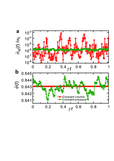
Figure 1: Time series of (a) the instantaneous shear stress, $\hat{\sigma}_{xy}(t)$, and (b) the instantaneous volume fraction $\hat{\varphi}(t)$, for $\dot{\gamma}=3.98\times 10^{-9}/\tau_{0}$ and $N=1000$. Green circles represent the results of constant pressure simulations with $P=10^{-5}\sigma_{0}$, while the red squares represent those of constant volume simulations with $\varphi=0.643$. Constant pressure simulations are superior as they yield small volume fraction fluctuations while drastically reducing the stress fluctuations.

Finally, we justify our choice to perform constant pressure simulations. The main motivation is to reduce the statistical uncertainty on the measurement of the physical observables of interest, which again results in more efficient simulations. In a finite system, physical observables may fluctuate differently depending on the statistical ensemble. In Fig. 1-a and Fig. 1-b we show typical time series of $\hat{\sigma}_{xy}(t)$ and $\hat{\varphi}(t)$, respectively, during constant pressure and constant volume simulations at a representative state point ($P=10^{-5}\sigma_{0}$, $\dot{\gamma}=3.98\times 10^{-9}/\tau_{0}$, $\varphi=0.643$, and $N=1000$). This figure indicates that the fluctuations of $\hat{\sigma}_{xy}(t)$ are considerably suppressed in constant pressure simulations by comparison with constant volume simulations, while those of $\hat{\varphi}(t)$ remain small enough. More quantitatively, we estimated the statistical uncertainty in the calculation of the viscosity and volume fraction. We divided the trajectory into 20 blocks making sure the size of the block ($=t_{\rm av}$) was larger than the typical correlation time and calculated the averages separately for each block. Then we evaluated the standard deviation of these block-averaged viscosities and densities. We found that the standard deviation of the viscosity is 5 times smaller in constant pressure simulations. On the other hand, the standard deviation of volume fraction by the ensemble average of three independent runs is as small as $3\times 10^{-4}$ at this state point, and it tends to decrease when $\varphi\to\varphi_{J}$. The uncertainty on $\varphi$ is small enough not to affect our scaling analysis (see for instance Fig. 7 below). Thus, we conclude that constant pressure simulations should be preferred for the purpose of an accurate determination of the viscosity $\eta(\varphi)$ near the jamming transition.

III Granular rheology in zero-pressure limit

III.1 Granular rheology

Let us start by presenting the flow behavior of our model of non-Brownian particles at finite pressure $P$ and finite $N$. We measure the average shear stress $\sigma_{xy}$, average volume fraction $\varphi$, and the viscosity $\eta$, as a function of the following three control parameters: $(P,N,\dot{\gamma})$.

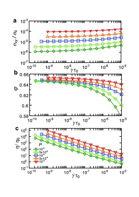
Figure 2: Evolution of our basic physical observables with the shear rate $\dot{\gamma}$ in steady state constant pressure simulations at different $P$ values for $N=10^{4}$: (a) shear stress $\sigma_{xy}$, (b) packing fraction $\varphi$, (c) shear viscosity $\eta$.

The three panels in Fig. 2 present these three observables as a function of $\dot{\gamma}$ at several pressures $P$ for a fixed system size of $N=10^{4}$ particles. As can be seen from Fig. 2-a, $\sigma_{xy}$ increases moderately with increasing $\dot{\gamma}$ at each given $P$, and it seems to converge to a finite value in the quasi-static limit $\dot{\gamma}\to 0$ in each case. By decreasing the pressure, the shear stress shifts vertically towards smaller values, but the overall shape of the curves remains essentially the same.

As shown in Fig. 2-b, the packing fraction decreases with increasing the shear rate in order for the pressure to remain constant, which is nothing but the well-known dilatancy effect bookyoel . For a given shear rate, the packing fraction increases weakly with increasing pressure due to the softness of the potential, because particles overlap more when the pressure increases. The packing fraction approaches a $P$- and $N$-dependent limit as $\dot{\gamma}\to 0$. At finite pressures this limiting packing fraction is above the jamming transition, so that particles overlap at rest and store a finite pressure in the static packing. In the $P\to 0,\dot{\gamma}\to 0$ limit, the overlap between the particles must vanish and the volume fraction converges to the jamming transition point, $\varphi_{J}$. The system size dependence is discussed in Sec. IV below.

Finally, let us focus on the behavior of the viscosity $\eta$ in Fig. 2-c. We find that the viscosity decreases rapidly with $\dot{\gamma}$ at constant pressure, mainly because the volume fraction also does. Clearly, the viscosity shifts systematically towards larger values as the pressure $P$ increases, because the density also increases.

It is important to notice that for the soft particle system under study, it is very difficult to distinguish between Newtonian and shear-thinning regimes from the data set presented in Fig. 2, because the viscosity is never a constant, contrary to more traditional measurements employing constant volume techniques teitel ; ikeda ; ikeda_soft . When density is constant, the rheology takes a different form below jamming (where it has Newtonian and shear-thinning behavior), and above jamming (where it has yield and shear-thinning behavior), and the pressure exhibits complex density and shear rate dependences teitel . When the pressure is constant these two regimes do not appear separately, as shown in Fig. 2. It is important to recall that although the two rheologies appear different, they are of course fully equivalent.

Since the total simulation time increases inversely with $\dot{\gamma}$, the results in Fig. 2-c indicate that simulations at small $P$ will achieve the same value of $\eta$ in a larger computational time than those at large $P$. However, as mentioned above, simulations at large $P$ are also more likely to be influenced by the softness of the potential, and presumably lie in the shear-thinning regime, as confirmed below. Because one of our main goals is to extract a wide range of viscosity data in the zero-pressure limit from finite pressure data, we will carefully analyze the role of particle softness (or, equivalently, finite pressures) in our results. Specifically, we must find our way between the following two constraints: on the one hand, low enough pressures are needed to attain the hard sphere limit; on the other hand, large pressures are more efficiently simulated. Thus, we will seek data which satisfy the hard sphere limit with the largest possible pressure.

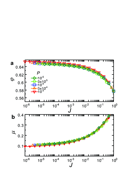
Figure 3: The shear stress and volume fraction from Fig. 2 are represented in a dimensionless form appropriate for non-Brownian hard spheres, Eqs. (11, 12). The symbols are as in Fig. 2. Deviations from full collapse originating from particle softness can be seen at large pressure, but are difficult to detect in this representation.

To analyze these data quantitatively, it is useful to use the zero pressure hard sphere limit as a reference point. In this limit, the rheology simplifies drastically, because the system does not contain any energy scale. Therefore, the imposed pressure determines simultaneously the appropriate stress and time scales governing the behavior of the system bookyoel ; GDRMiDi ; chevoir . As is well-known in the literature of granular materials, this suggests to introduce dimensionless rheological quantities, and to express the shear stress and shear rates in dimensionless forms, since the packing fraction is already a non-dimensional quantity. Following the usual notations bookyoel , we define the friction coefficient as a dimensionless shear stress scale

$$\mu=\frac{\sigma_{xy}}{P},$$ (10)

and the viscous number as a dimensionless shear rate scale,

$$J=\frac{\dot{\gamma}\eta_{0}}{P}.$$ (11)

In the zero pressure limit, we expect therefore that the rheology is expressed through two simple relations bookyoel ,

$$\mu=\mu(J),\quad\varphi=\varphi(J),$$ (12)

from which the shear viscosity is directly deduced as:

$$\frac{\eta}{\eta_{0}}=\frac{\mu(J)}{J}.$$ (13)

An important conclusion is that since the relation $\varphi(J)$ can be inverted, $J=J(\varphi)$, the shear viscosity becomes a unique function of the volume fraction, $\eta(\varphi)/\eta_{0}=\mu(J(\varphi))/J(\varphi)$, and in particular it does not depend on the imposed shear rate. In this limit, the rheology of the suspension is therefore purely Newtonian.

In Fig. 3, we use these rescaled variables for our finite pressure simulations, and find that an essential part of the pressure dependence is scaled out by this scaled representation of the data, compare with Fig. 2. Although deviations from this scaling can be seen, for instance, for the largest pressure value, the data collapse look overall quite good. This is somewhat surprising as soft repulsive particles display strong shear-thinning effects near the jamming transition, as we discuss below. We are led to conclude that this presentation of the data is actually a poor test of the influence of the particle softness (or other perturbations to the hard sphere interaction), in particular when statistical noise becomes significant, as is inherent for instance to experimental measurements. As we show below, a different representation of the data is therefore recommended.

III.2 Taking the zero-pressure limit

Although the data collapse in Fig. 3 looks good, it is difficult to see how the data deviate from the hard-sphere behavior. In order to observe and quantify these deviations more precisely, we study, for each value of $J$, the maximal pressure above which the data for $\mu(P,J,N)$ and $\varphi(P,J,N)$ start to deviate from the $P\to 0$ limit, for a given system size $N$. We then fit the $P$-independent parts of the data to the following functional forms bookyoel ; GDRMiDi ; Lespiat ; roux ; Lerner :

$$\varphi(P\to 0,J,N) =\varphi_{J}(N)-C_{\varphi}(N)J^{b_{\varphi}},$$ (14)

$$\mu(P\to 0,J,N) =\mu_{J}(N)+C_{\mu}(N)J^{b_{\mu}},$$ (15)

where we explicitly included a system size dependence, which is the subject of Sec. IV.

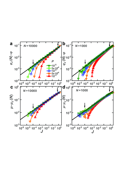
Figure 4: Log-log representation of the power law convergence of the friction coefficient and volume fraction to their static values as the viscous number $J$ is decreased. The power laws in Eq. (14, 15) appear as black straight lines. In each panel, black arrows delimit the range of data where the zero-pressure limit is measured, and used for fits to Eqs. (14, 15). Data are presented for two different system sizes.

The results of this zero-pressure analysis are presented in Fig. 4 for two system sizes, $N=10^{4}$ and $N=10^{3}$. We show the $J$-dependence of $\varphi_{J}(N)-\varphi(P,J,N)$ and $\mu_{J}(N)-\mu(P,J,N)$ in a log-log scale. This amounts to representing the (nearly) collapsed data in Fig. 3 using a logarithmic rather than linear representation of the vertical axis. In this different representation, finite pressure deviations are systematic and become much easier to detect both for $\mu$ and for $\varphi$.

From the figure we see that deviations arise for $J$ lower than a crossover value that vanishes as $P\to 0$, by construction. In Fig. 4, we delimit by two vertical arrows the range of viscous numbers $J$ where the $P=0$ limit is actually reached within the statistical accuracy of the data, and where the ‘envelope’ of the converged data can be analyzed. By fitting this envelope to the functional forms given in Eqs. (14, 15), we deduce for each system size $N$ the fitting parameters involved in these expressions. The result of these fit are indicated by full lines in Fig. 4. They describe a power law convergence of $\varphi$ and $\mu$ towards their $J\to 0$ asymptotic values. We emphasize that these power laws are obeyed over a significant range of inertial numbers $J$ of about 4 decades, and we find that these power laws hold independently for each different system size studied numerically, $N=10^{2}-10^{4}$.

IV Large-$N$ limit of granular rheology

IV.1 ‘Brute-force’ analysis of numerical data

Having dealt with the zero-pressure limit, we now proceed to evaluate quantitatively the $N\to\infty$ limit, so as to get rid of finite size effects. Finite size effects have been discussed in earlier simulations of non-Brownian particle systems roux ; ohern1 ; ohern2 ; pinaki ; recent_teitel ; otherteitel ; otherteitel2 .

In Fig. 5 we show the $N$-dependence of the parameters $\varphi_{J}(P\to 0,N)$, $C_{\varphi}(N)$, $b_{\varphi}(N)$, $\mu_{J}(P\to 0,N)$, $C_{\mu}(N)$, and $b_{\mu}(N)$, defined in Eqs. (14, 15), and obtained from independently fitting the data shown Fig. 4 for different system sizes. The fact that these parameters evolve smoothly with system size demonstrates the high quality of our numerical data, since these parameters are measured from statistically independent sets of data.

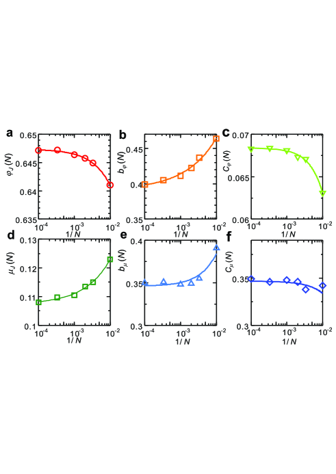
Figure 5: System size dependence of the fitting parameters appearing in Eqs. (14, 15). The lines are fits describing a power law approach to the asymptotic $N\to\infty$ limit, as in Eq. (16), with values reported in Table 1.

We find empirically that the system size dependence of these parameters is also well described by power laws

$${\cal O}(N)={\cal O}(N\to\infty)+{A_{\cal O}}{N^{-\alpha_{\cal O}}},$$ (16)

where ${\cal O}(N)$ stands for any of the observables under study measured for a finite $N$, ${\cal O}(N\to\infty)$ its fitted asymptotic value assuming a power law convergence with $N$ with an exponent $\alpha_{\cal O}$.

It is not surprising that such power laws are obeyed because these parameters change very little when the total number of particles is increased by two orders of magnitude. These power laws can thus be seen at this stage as a convenient empirical method to determine quantitatively the asymptotic value of the parameters entering the granular rheology. The extrapolation to infinite system size eventually allows us to obtain the asymptotic behavior of the system as both the hard sphere (zero-pressure) and thermodynamic limits are taken, $N\to\infty,P\to 0$. The full set of fitting parameters used in Fig. 5 are summarized in Table 1.

${\cal O}(N)$	$\varphi_{J}$	$b_{\varphi}$	$C_{\varphi}$	$\mu_{J}$	$b_{\mu}$	$C_{\mu}$
${\cal O}(N\to\infty)$	0.6474	0.391	0.0683	0.108	0.346	0.347
$A_{\cal O}$	-0.323	0.756	-1.15	0.279	2.93	-1.44
$\alpha_{\cal O}$	0.852	0.505	1.17	0.626	0.946	1.02

Table 1: Sets of parameters obtained by fitting the system size dependence of several physical observables with the functional form in Eq. (16).

In particular, our data indicate that in the double limit $N\to\infty,P\to 0$, the asymptotic granular rheology of the present binary system reads:

$$\varphi=\varphi_{J}-C_{\varphi}J^{b_{\varphi}},\quad\mu=\mu_{J}+C_{\mu}J^{b_{\mu}},$$ (17)

with the estimated asymptotic values:

$$\varphi_{J} =0.6474,\quad b_{\varphi}=0.391,$$ (18)

$$\mu_{J} =0.108,\quad b_{\mu}=0.346.$$ (19)

IV.2 Scaling analysis: Diverging correlation length

It is fruitful to revisit the above extrapolation to infinite system sizes using a somewhat simpler, but physically more illuminating, scaling analysis. Using the results of the above ‘brute force’ fitting procedure to extract the large-$N$ limit of the results, we can represent in Fig. 6-a the dependence of $\varphi_{J}(N\to\infty)-\varphi$ and in Fig. 6-b the dependence of $\mu_{J}(N\to\infty)-\mu$ for the data measured in the zero-pressure limit. It is important to note that we use the infinite system size asymptotic values $\varphi_{J}(N\to\infty)$ and $\mu_{J}(N\to\infty)$ to represent data at finite $N$, an approach which reveals finite size effects more clearly. Recall also that these measurements are obtained in the zero-pressure limit, as we are only concerned with finite size effects in the present subsection.

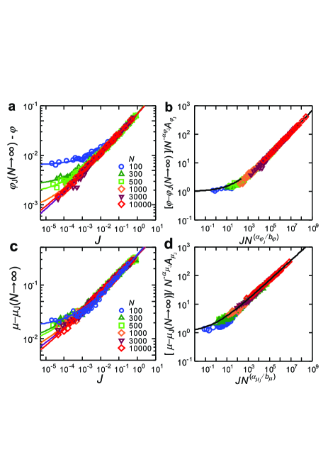
Figure 6: Scaling analysis of finite size effects. (a) Emergence of finite size effects for the volume fraction $\varphi$, and (c) for the friction coefficient $\mu$. The solid lines represent fits using Eqs. (16, 17). (b) Scaling plot for the volume fraction using Eq. (22). (d) Scaling plot for the friction coefficient using Eq. (23). Solid lines in (b, d) use parameters in Table 1.

In the different representation of Fig. 6, finite size corrections to the asymptotic behavior can be better appreciated and they seem to take a particularly simple and suggestive form. For a given system size, the data exhibit two distinct regimes. For large $J$, the data show little size dependence, while at small $J$ clear deviations are observed. Additionally, the crossover viscous number separating the two regimes strongly depends on $N$, the deviations shifting to smaller $J$ values as $N$ increases and disappearing as $N\to\infty$, by construction.

This qualitative description suggests that finite size effects can be described analytically using the following scaling form:

$$\varphi(J,N) =[\varphi_{J}(N\to\infty)+A_{\varphi_{J}}N^{-\alpha_{\varphi_{J}}}]-C_{\varphi}J^{b_{\varphi}},$$ (20)

$$\mu(J,N) =[\mu_{J}(N\to\infty)+A_{\mu_{J}}N^{-\alpha_{\mu_{J}}}]+C_{\mu}J^{b_{\mu}},$$ (21)

which amounts to neglecting the system size dependence of the prefactors $C_{\varphi}$ and $C_{\mu}$ and the exponents $b_{\varphi}$ and $b_{\mu}$ in the ‘brute force’ description of Sec. IV.1. The physical content of Eqs. (20, 21) is that a finite size system obeys the asymptotic granular rheology of Eqs. (17), but with values for the jamming density $\varphi_{J}$ and the friction coefficient $\mu_{J}$ which are ‘renormalized’ by finite size corrections. In particular, this implies that smaller systems jam at a smaller density, Fig. 5-a, with a larger value of the friction coefficient, Fig. 5-b. This description is fully consistent with earlier work ohern1 ; roux .

This simplification then suggests that the finite size data can be collapsed using the following representation:

$$\frac{\varphi(J,N)-\varphi_{J}(N\to\infty)}{A_{\varphi_{J}}N^{-\alpha_{\varphi_{J}}}} ={\cal F}_{\varphi}(JN^{\alpha_{\varphi_{J}}/b_{\varphi}}),$$ (22)

$$\frac{\mu(J,N)-\mu_{J}(N\to\infty)}{A_{\mu_{J}}N^{-\alpha_{\mu_{J}}}} ={\cal F}_{\mu}(JN^{\alpha_{\mu_{J}}/b_{\mu}}),$$ (23)

where ${\cal F}_{\varphi}(x)$ and ${\cal F}_{\mu}(x)$ are two scaling functions with the asymptotic behavior ${\cal F}_{\varphi,\mu}(x\to 0)=1$ (when finite size effects dominate), and ${\cal F}_{\varphi,\mu}(x\to\infty)\sim x^{b_{\varphi,\mu}}$ (when finite size effects are absent).

The scaling plots resulting from Eqs. (22, 23) for $\varphi$ and $\mu$ are shown in Figs. 6-b and Fig. 6-d, respectively. We can see that our scaling hypothesis describes the data in a satisfactory manner. The full lines in the figures are from the fitted values obtained above in Sec. IV.1, see Table 1, and provide an acceptable analytical description of the numerical results over a broad range of scaled variables.

Remarkably, this data collapse suggests that the approach to the jamming transition as $J\to 0$ in non-Brownian hard particles under shear is accompanied by a diverging length scale, $\xi(J\to 0)\to\infty$. From the above scaling, we deduced that for each system size, there exists a crossover $J$-value below which finite size effects are observed. This can be interpreted by saying that finite size effects are observed whenever $\xi(J)$ becomes comparable to the linear size of the system, $\xi\sim N^{1/d}$, where $d$ is the space dimensionality. Combining this argument to the scaling forms in Eqs. (22, 23) suggests that

$$\xi\sim J^{-\nu},$$ (24)

with $\nu\approx b_{\varphi}/(\alpha_{\varphi_{J}}d)\approx b_{\mu}/(\alpha_{\mu_{J}}d)$. From the values reported in Table 1 we obtain $\nu\approx 0.153$ (from $\varphi$) and $\nu\approx 0.184$ (from $\mu$). These numerical estimates are consistent with a unique value for $\nu$. Note that the reliability of this scaling analysis depends on the validity of the assumption that both the pair of exponents $b_{\mu}$ and $b_{\varphi}$ and the pair of coefficients $C_{\mu}$ and $C_{\varphi}$ are independent of the system size $N$. The data in Fig. 5 show that $b_{\mu}$ and $C_{\mu}$ are actually nearly independent of $N$, so that the value $\nu\approx 0.184$ is probably more reliable.

To discuss the value of this exponent, it is useful to first remember that once the zero-pressure limit has been taken, the jamming transition at $\varphi_{J}$ is approached along a specific path, namely, as the rescaled shear rate goes to zero, $J\to 0$. This is therefore a different path in control parameters space from more traditional approaches where for instance static packings ($J=0$) are produced at densities approaching $\varphi_{J}$ from below ohern2 , or where the shear rate is decreased exactly at the jamming density recent_teitel . In the present case, the packing fraction is actually also changing along the way.

We can nevertheless compare the obtained value for $\nu$ to a number of literature results. First we notice that the rather small value of the exponent $\nu$ in Eq. (24) is consistent with a recent discussion of the correlation length characterizing the response to a local perturbation in a similar numerical model during ; degiuli , where the value $\nu\approx 0.15$ is reported. A second set of approaches dealing with the rheology of dense amorphous materials has demonstrated the need to introduce a correlation length in dense flows to account for the emergence of ‘non-local’ rheological effects KEP ; kamrin ; bruno . Despite the diversity of empirical models, they all introduce a lengthscale $\xi_{nl}$ which diverges at jamming as a square root of the distance to yielding, $\xi_{nl}\sim(\mu-\mu_{J})^{-1/2}$. Converting our findings in this representation, we obtain $\xi\sim J^{-\nu}\sim(\mu-\mu_{J})^{-\nu/b_{\mu}}$, where $\nu/b_{\mu}=1/(\alpha_{\mu_{J}}d)\approx 0.53$. The close agreement between our findings and these empirical models (adjusted to best fit numerical data) suggests a possible deep connection between the finite size effects we detect directly in our work, and non-local effects observed experimentally. To our knowledge, the correlation length exponent has not been directly determined experimentally olivier , but we note that the smallness of $\nu$ means that $\xi$ diverges relatively slowly as the jamming transition is approached. This probably implies that it should be difficult to measure $\nu$ experimentally, unless the system is extremely close to jamming Pouliquen ; Lespiat .

IV.3 Asymptotic results for the shear viscosity

Having obtained ‘converged’ numerical results for the packing fractions and the friction coefficient, i.e. data that satisfy both the hard sphere ($P\to 0$) and the large system size limit ($N\to\infty$), we can now evaluate the physical behavior of the shear viscosity in the limit where neither particle softness nor finite size effects play any role.

To this end, we combine the converged values of $\mu$ and $\varphi$ and use Eq. (13) to obtain the shear viscosity. In Fig. 7, we represent $\eta$ as a function of $\varphi_{J}-\varphi$ for several finite pressures and system sizes, carefully collecting the data that satisfy both $P\to 0$ and $N\to\infty$ limits. Our numerical measurements cover about 5 orders of magnitude in viscosity, which is significantly larger than the typical range accessed experimentally and in earlier simulation studies andreotti ; ikeda ; OlssonTeitel2012 .

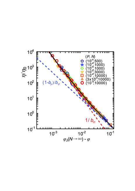
Figure 7: Shear viscosity after the hard sphere ($P\to 0$) and the large system size ($N\to\infty$) limits are taken. Symbols are measurements for different $N$ and $P$ which satisfy the $N\to\infty,P\to 0$ limits. The black line represents Eq. (25) with parameters taken from Table 1. Red and blue dashed lines separately represent the two power law contributions in Eq. (25).

Collecting the above results, we can easily get an analytical description of these viscosity data by combining Eq. (17) with Eq. (13), so that the relationship between $\eta$ and $\varphi$ in the $P\to 0$ and $N\to\infty$ limits reads:

$$\frac{\eta}{\eta_{0}}=\mu_{J}\left[\frac{C_{\varphi}}{\varphi_{J}-\varphi}\right]^{\frac{1}{b_{\varphi}}}+C_{\mu}\left[\frac{C_{\varphi}}{\varphi_{J}-\varphi}\right]^{\frac{1-b_{\mu}}{b_{\varphi}}},$$ (25)

where all parameters should be taken with their $N\to\infty$ values (we have omitted this limit in Eq. (25) to simplify the notation). Using the numerical values reported in Table 1, we can directly compare the analytical expression in Eq. (25) to the numerical data. This is shown as the the black line going through the symbols in Fig. 7. The very good agreement confirms the consistency of our data analysis.

We note that Eq. (25) differs from the single power law function, which was used in several previous studies Pouliquen ; teitel ; andreotti ; Claudin to fit viscosity data, but is mathematically consistent with the description of corrections to scaling in Ref. otherteitel2 . The viscosity behaves in fact as the sum of two power laws with different exponents, such that taking the final limit of $J\to 0$ in our data, we obtain the asymptotic behavior where the largest of the two exponents dominate:

$$\eta\sim(\varphi_{J}-\varphi)^{-1/b_{\varphi}}\sim(\varphi_{J}-\varphi)^{-2.55}.$$ (26)

Our numerical analysis, which considerably expand previous work, confirms the robustness of the algebraic divergence of the shear viscosity in non-Brownian hard particles near the jamming density. In particular, we detect no sign of a crossover towards a sharper density dependence, as observed in thermalized assemblies of hard particles gio . This different qualitative behavior between Brownian and non-Brownian suspensions confirms the distinct nature of glass and jamming transitions in colloidal assemblies tom ; ikeda ; PZ .

In Fig. 7, the two power law contributions in Eq. (25) are separately highlighted with dashed lines. It is clear that the shear viscosity crosses over from one power law divergence to another, the crossover between the two occurring relatively close to the jamming transition, for $\Delta\varphi\approx 0.02$. This implies that a precise determination of the critical exponent governing the viscosity divergence is challenging, as the scaling regime starts at the lower boundary of the regime explored in the most recent experiments Pouliquen . This finding might also explain the diversity of critical exponents $\beta$ that have been reported in the literature, because a power law fit of a narrower range of data could yield an exponent lying anywhere in the range of $\beta\in[(1-b_{\mu})/b_{\varphi},1/b_{\varphi}]\approx[1.67,2.55]$. This is broadly consistent with the rough accepted value $\beta\approx 2$ found in many previous works Pouliquen ; teitel ; andreotti ; Claudin , but somewhat smaller than the recent prediction $\beta=2.83$ for its numerical value degiuli .

V Soft granular rheology

V.1 Scaling hypothesis for soft grains

Because of the finite energy scale introduced by the particle softness, the rheology of soft particles is not uniquely governed by the viscous number $J$, and non-linear effects therefore come in, as described in Fig. 4. In this section, we shall study the effect of particle softness or, equivalently, of finite pressures. We shall present detailed results for two system sizes to establish the robustness of our analysis, but we do not explicitly account for the finite size dependence of physical observables as we did for the zero-pressure limit. The main variable of interest in this section is therefore the pressure $P$. Note that in this section, the specific choice of a harmonic repulsion between the particles becomes relevant.

The finite pressure corrections to the granular rheology shown in the data of Fig. 4 are very suggestive, and qualitatively reminiscent of the finite size effects shown in Fig. 6. Indeed these data show that for a given pressure value, the data at large $J$ are not affected by $P$, while deviations are seen at small enough $J$. Crucially, the crossover $J$-value separating the two regimes is pressure dependent, and vanishes, by construction, when $P\to 0$.

Inspired by the scaling hypothesis performed in Sec. IV.2 to account for finite size effects, we make a similar hypothesis for finite pressure and assume that finite pressure corrections can be analytically accounted for by generalizing the granular rheology in Eq. (17) to the following ‘soft granular rheology’:

$$\varphi(P,J) =\varphi_{J}(P)-C_{\varphi}J^{b_{\varphi}},$$ (27)

$$\mu(P,J) =\mu_{J}(P)+C_{\mu}J^{b_{\mu}},$$ (28)

where $\varphi$ and $\mu$ are measured at finite pressures $P$ and viscous numbers $J$. Comparing to Eq. (17), these expressions capture the idea that a finite pressure simply ‘renormalizes’ the hard sphere jamming density $\varphi_{J}$ and friction coefficient $\mu_{J}$ to pressure dependent values, while the functional form of the rheology is unaffected.

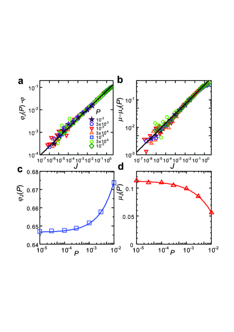
Figure 8: Test of the soft granular rheology extending the hard sphere rheology to soft particles. Data are shown for $N=10^{3}$. (a) $\varphi_{J}(P)-\varphi$ vs. $J$ for several $P$ values; the solid line represents Eq. (27). (b) $\mu_{J}(P)-\mu$ vs. $J$ for several $P$ values; the solid line represents Eq. (28). (c) Pressure dependence of $\varphi_{J}(P)$; the solid line represents Eq. (29) with $x=0.75$. (d) Pressure dependence of $\mu_{J}(P)$; the solid line represents Eq. (30) with $y=0.56$.

We test this very simple idea in Figs. 8-a,b where we represent $\varphi_{J}(P,J)-\varphi$ and $\mu(P,J)-\mu_{J}(P)$ as functions of the viscous number $J$ for different pressure values. To construct these figures, we determine for each pressure the values of $\varphi_{J}(P)$ and $\mu_{J}(P)$ that yield the best collapse of the data. Clearly, this procedure removes the systematic pressure dependencies observed in Fig. 4, which shows that our hypothesis in Eqs. (27, 28) is satisfied within the statistical accuracy of our data.

The measured functions $\varphi_{J}(P)$ and $\mu_{J}(P)$ are reported in Figs. 8-c,d. These data show that finite pressure effects can be described by a shift of the jamming density $\varphi_{J}(P)$ and the friction coefficient $\mu_{J}(P)$. Empirically, we find that these deviations from the hard sphere values $\varphi_{J}(P\to 0)$ and $\mu_{J}(P\to 0)$ are well described by the following formula:

$$\varphi_{J}(P) =\varphi_{J}(0)+c_{\varphi}P^{x},$$ (29)

$$\mu_{J}(P) =\mu_{J}(0)-c_{\mu}P^{y},$$ (30)

The numerical values of the two new exponents entering Eqs. (29) and (30) are $x\approx 0.75$ and $y\approx 0.56$, obtained by fitting over the entire pressure range. The fits are shown as lines in Figs. 8-c,d. The precise value of these exponents depend on the chosen repulsive force (with $\alpha_{r}=2$) between the soft particles.

The extension of the traditional granular rheology to soft particles is based on the simple physical idea that soft particles behave very much as hard particles, but with a ‘renormalized’ particle diameter and friction coefficient. Therefore, this approach is similar to earlier attempts to describe the rheology OlssonTeitel2012 and thermal dynamics tom of soft particles in terms of the corresponding hard sphere system.

The soft granular rheology in Eqs. (27, 28) suggests that rheological measurements performed at constant pressure (rather than constant density) would yield results essentially indistinguishable from zero pressures. In other words, detecting softness effects seems challenging in a traditional granular experimental setting. In particular, the viscosity of a non-Brownian suspensions of soft particles measured at constant pressure would diverge with the same power law as for hard grains, but at a slightly higher packing fraction.

The main new effect introduced by the particle softness is the possibility to explore states which are above the jamming transition, thus allowing a description of the constant density rheology of the solid phase above $\varphi_{J}$. In fact, by taking the zero shear rate limit in Eqs. (27, 28) we find that for finite $P$, the volume fraction converges to a value larger than $\varphi_{J}(P\to 0)$ (yielding a compressed packing of soft particles) supporting a finite yield stress, $\sigma_{Y}$. From Eqs. (29, 30), we obtain the following analytic form:

$$\sigma_{Y}=\left[\frac{\varphi-\varphi_{J}(0)}{c_{\varphi}}\right]^{\frac{1}{x}}\left[\mu_{J}(0)-c_{\mu}\left(\frac{\varphi-\varphi_{J}(0)}{c_{\varphi}}\right)^{\frac{y}{x}}\right].$$ (31)

This expression shows that the yield stress vanishes asymptotically as a power law as the jamming density is approached, $\sigma_{Y}\sim(\varphi-\varphi_{J})^{\alpha}$, where $\alpha=1/x\approx 1.33$. However, much as for the shear viscosity, we find that the yield stress is actually the sum of two distinct power laws with exponents $1/x$ and $(1+y)/x$, the latter being asymptotically sub-dominant. Values of the yield stress exponents in the range $\alpha=1.1-1.5$ have been reported before teitel ; recent_teitel ; brian ; hatano2 .

The soft granular rheology in Eqs. (27, 28) allows us to describe the rheology of non-Brownian soft particles on both sides of the jamming transition accounting at once for a diverging viscosity below $\varphi_{J}$ and the emergence of a finite yield stress above $\varphi_{J}$, with non-trivial shear-thinning regimes at larger shear rates. A clear advantage of the present description is that it naturally incorporates the rheology of hard non-Brownian spheres as a well-defined reference point, which is automatically recovered in the limit of infinitely hard particles.

V.2 Comparison with the original Olsson and Teitel analysis

We now compare the soft granular rheology in Eqs. (27, 28) to previous work. A qualitatively similar scaling analysis of the rheology of soft particles was proposed by Olsson and Teitel in Ref. teitel . It has then often been used to organize numerical and experimental data obtained in non-Brownian soft suspensions teitel ; OlssonTeitel2012 ; nordstrom ; jose .

This approach was motivated by an idea similar to the one used in the previous section, namely an extension of the hard particle limit to soft particles. The Olsson-Teitel analysis relies on essentially three assumptions footnote : (i) the viscosity of hard particles diverges as a power law when the volume fraction approaches the jamming transition density: $\eta\propto(\varphi_{J}-\varphi)^{-\beta}$; (ii) a finite yield stress is obtained above the jamming transition which increases as a power law: $\sigma_{Y}\propto(\varphi-\varphi_{J})^{\alpha}$. (iii) these two regimes can be connected by scaling. Mathematically, these assumptions yield the following model for the critical properties of soft particles near jamming:

$$\sigma_{xy}=|\varphi-\varphi_{J}|^{\alpha}{\cal G}_{\pm}\left(\frac{\dot{\gamma}}{|\varphi-\varphi_{J}|^{\alpha+\beta}}\right),$$ (32)

with the following asymptotic forms for the scaling functions: ${\cal G}_{+}(x\to 0)\sim const.$ (emergence of a yield stress), ${\cal G}_{-}(x\to 0)\sim x$ (Newtonian regime with diverging viscosity), ${\cal G}_{\pm}(x\to\infty)\sim x^{\alpha/(\alpha+\beta)}$ (emergence of a critical shear-thinning regime). This mathematical model implies that exactly at the jamming transition, $\varphi=\varphi_{J}$, the rheology is described by a nontrivial power law, $\sigma\sim\dot{\gamma}^{\alpha/(\alpha+\beta)}$ corresponding to shear-thinning behavior. This model is appealing as it also directly connects to the well-known (empirical) Herschel-Bulkley rheology wagner ; OlssonTeitel2012 . The scaling form in Eq. (32) therefore makes the simple assumption that the three regimes (Newtonian, yield stress, shear-thinning) are connected by smooth functions.

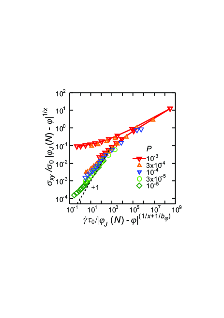
Figure 9: Test of the scaling plot Eq. (32) for $N=10^{4}$ with exponents $\alpha=1/x\approx 1.33$ from Eq. (31) and $\beta=1/b_{\varphi}\approx 2.55$ from Eq. (25). Deviations from perfect collapse are observed.

While very similar in spirit, the soft granular rheology we propose in Eqs. (27, 28) yields a model which is mathematically different from Eq. (32), although some asymptotic behaviors are the same. For instance, both models predict an asymptotic power law divergence of the Newtonian viscosity, power law emergence of the yield stress, and algebraic critical shear-thinning regime. However, as we already pointed out, we find that both the Newtonian viscosity and the yield stress are described by the sum of two power laws, see Eqs. (25, 31). A direct consequence of our model is that the rheology at the jamming density is described by a sum of three power laws, rather than a single one. More importantly perhaps, all the asymptotic behaviors incorporated in our model cannot be simply connected by scaling functions as in Eq. (32).

We acknowledge that our conclusions are consistent with the more recent description of the shear rheology near jamming by Olsson and Teitel themselves, which includes ‘corrections to scaling’ otherteitel2 ; note . These corrections to scaling are shown to affect the data collapse suggested by Eq. (32), and naturally predict that simple algebraic divergences become sums of power laws, in agreement with our findings. A similar statement is made more explicitely in other works brian , which also imply that the appealing data collapse predicted by Eq. (32) can only be approximate. In Fig. 9, we confirm that our extended set of data cannot be collapsed on two branches, using the scaling form in Eq. (32). To build this diagram, we used asymptotic exponents for the yield stress and the shear viscosity determined from our simulations. We respectively use $\alpha=1/x$ obtained from Eq. (31) and $\beta=1/b_{\varphi}$ obtained from Eq. (25), together with our best estimate for the jamming density $\varphi_{J}$. We have tried to use the freedom offered by Eq. (32) to shift these numbers from their actual values and used effective exponents and shifted critical density to improve the quality of the data collapse. We find that the data collapse cannot be significantly improved, in the sense that improving the quality of the collapse in one part of the plot deteriorates the quality in another part of the plot, and acceptable collapse cannot be achieved for the entire data set. These conclusions are also supported by direct analysis of the mathematical model in Eqs. (27, 28) using numerical values determined from the simulations, where deviations from scaling can be analysed more finely. We conclude that an apparent scaling of the data must result from the simultaneous use of a smaller dynamic range and of effective values for critical exponents.

VI Summary and conclusions

In this work we have optimized a simple numerical approach using non-Brownian soft particles to analyze in detail the rheology of non-Brownian suspensions over a very wide dynamic range, paying attention to finite size effects. This allowed us to confirm the algebraic divergence of the Newtonian viscosity of suspensions of hard particles and to point out the difficulty of corresponding experimental measurements. Through a finite size scaling analysis, we have also established the existence of a correlation length scale that diverges as the jamming transition is approached.

We then used these results to extend the precise hard sphere rheology obtained numerically to describe the non-linear rheology of soft particle suspensions across the jamming transition, which we coined soft granular rheology. Although very simple and natural from the viewpoint of granular materials, our approach yields a mathematical model which differs from earlier attempts at a scaling description. Because it starts from the natural ‘granular’ variables $\mu$ and $\varphi$, our approach suggests that no simple scaling form exists for the shear viscosity of soft suspensions.

In future work we would like to explore in more detail the connection between the correlation length revealed in this work and the non-local rheological effects which are currently receiving growing attention KEP ; kamrin ; bruno . Another relevant issue concerns the role of frictional forces in hard particle systems. It would be very interesting to extend the present study to include frictional forces, and see how our numerical results for the asymptotic behavior of frictionless particles are affected by friction. This would be very valuable to compare with experimental results performed with real granular suspensions where friction is unavoidable.

- (1) H. M. Jaeger, S. R. Nagel, and R. P. Behringer, Rev. Mod. Phys. 68, 1259 (1996).
- (2) T. G. Mason, J. Bibette, and D. A. Weitz, J. Colloid Interface Sci. 179, 439 (1996).
- (3) J. Mewis and N. J. Wagner, Colloidal Suspension Rheology (Cambridge University Press, 2012).
- (4) F. Boyer, E. Guazzelli, and O. Pouliquen, Phys. Rev. Lett. 107, 188301 (2011).
- (5) B. Hertzhft, S. Kakadjian, and M. Moan, Colloid Surf. A 263, 153 (2005).
- (6) L. Berthier and G. Biroli, Rev. Mod. Phys. 83, 587 (2011).
- (7) M. van Hecke, J. Phys. Condens. Matter 22, 033101 (2010).
- (8) B. Andreotti, Y. Forterre, and O. Pouliquen, Granular media: between fluid and solid (Cambridge University Press, Cambridge, 2013).
- (9) C. Bonnoit, T. Darnige, E. Clement, and A. Lindner, J. Rheol. 54, 65 (2010).
- (10) B. Andreotti, J.-L. Barrat, and C. Heussinger, Phys. Rev. Lett. 109, 105901 (2012)
- (11) P. Olsson and S. Teitel, Phys. Rev. Lett. 99, 178001 (2007).
- (12) M. Trulsson, B. Andreotti, and P. Claudin, Phys. Rev. Lett. 109, 118305 (2012).
- (13) E. Lerner, G. Düring, and M. Wyart, Proc. Natl. Acad. Sci. U. S. A., 109, 4798 (2012).
- (14) I. M. Krieger and T. J. Dougherty, Trans. Soc. Rheol. 3, 137 (1959).
- (15) I. M. Krieger, Adv. Colloid Interface Sci. 3, 111 (1972).
- (16) L. E. Silbert, D. Ertas, G. S. Grest, T. C. Halsey, and D. Levine, Phys. Rev. E 65, 031304 (2002).
- (17) H. P. Zhang and H. A. Makse, Phys. Rev. E 72, 011301 (2005).
- (18) K. Shundyak, M. van Hecke, and W. van Saarloos, Phys. Rev. E 75, 010301(R) (2007).
- (19) M. Otsuki and H. Hayakawa, Phys. Rev. E 83, 051301 (2011).
- (20) N. Huang, G. Ovarlez, F. Bertrand, S. Rodts, P. Coussot, and D. Bonn, Phys. Rev. Lett. 94, 028301 (2005).
- (21) S. Manneville, Rheol Acta 47, 301 (2008).
- (22) G. Brambilla, D. El Masri, M. Pierno, G. Petekidis, A. B. Schofield, L. Berthier, and L. Cipelletti, Phys. Rev. Lett. 102, 085703 (2009).
- (23) R. G. Larson, The Structure and Rheology of Complex Fluids (New York: Oxford University Press, 1999).
- (24) R. Höhler and S. Cohen-Addad, J. Phys. Condens. Matter 17, R1041 (2005).
- (25) A. Ikeda, L. Berthier, and P. Sollich, Phys. Rev. Lett. 109, 018301 (2012).
- (26) P. Olsson and S. Teitel, Phys. Rev. Lett. 109, 108001 (2012).
- (27) A. Ikeda, L. Berthier, and P. Sollich, Soft Matter 9 7669 (2013).
- (28) L. Berthier and T. A. Witten, EPL 86, 10001 (2009); Phys. Rev. E 80, 021502 (2009).
- (29) P. Olsson and S. Teitel, Phys. Rev. E 83, 030302(R) (2011).
- (30) D. J. Durian, Phys. Rev. Lett. 75, 4780 (1995).
- (31) C. S. O’Hern, S. A. Langer, A. J. Liu, and S. R. Nagel, Phys. Rev. Lett. 88, 075507 (2002).
- (32) C. S. O’Hern, L. E. Silbert, A. J. Liu, and S. R. Nagel, Phys. Rev. E 68, 011306 (2003).
- (33) T. Hatano, J. Phys. Soc. Jpn. 77, 123002 (2008).
- (34) E. Lerner, G. During, and M. Wyart, Comp. Phys. Commun. 184, 628 (2013).
- (35) D. Vagberg, D. Valdez-Balderas, M. A. Moore, P. Olsson, and S. Teitel, Phys. Rev. E 83, 030303(R) (2011).
- (36) M. Allen and D. Tildesley, Computer Simulation of Liquids (Oxford University Press, Oxford, 1987).
- (37) D. Vagberg, P. Olsson, and S. Teitel, Phys. Rev. Lett. 113, 148002 (2014).
- (38) S. E. Feller, Y. Zhang, R. W. Pastor, and B. R. Brooks, J. Chem. Phys. 103, 4613 (1995).
- (39) A. Kolb and B. Dunweg, J. Chem. Phys. 111, 4453 (1999).
- (40) M. Tuckerman, B. J. Berne, and G. J. Martyna, J. Chem. Phys. 97, 1990 (1992).
- (41) GDR MiDi, Eur. Phys. J. E 14, 341 (2004).
- (42) F. da Cruz, S. Emam, M. Prochnow, J.-N. Roux, and F. Chevoir, Phys. Rev. E 72, 021309 (2005).
- (43) R. Lespiat, S. Cohen-Addad, and R. Höhler, Phys. Rev. Lett. 106, 148302 (2011).
- (44) P.-E. Peyneau and J.-N. Roux, Phys. Rev. E 78, 011307 (2008).
- (45) P. Chaudhuri, L. Berthier, and S. Sastry, Phys. Rev. Lett. 104, 165701 (2010).
- (46) G. Düring, E. Lerner, and M. Wyart, Phys. Rev. E 89, 022305 (2014).
- (47) E. DeGiuli, G. Düring, E. Lerner, and M. Wyart, arXiv:1410.3535.
- (48) L. Bocquet, A. Colin and A. Ajdari, Phys. Rev. Lett. 103, 036001 (2009).
- (49) D. L. Henann and K. Kamrin, Proc. Natl. Acad. Sci. USA 110, 6730 (2013).
- (50) M. Bouzid, M. Trulsson, P. Claudin, E. Clément, and B. Andreotti, Phys. Rev. Lett. 111, 238301 (2013).
- (51) O. Pouliquen, Phys. Rev. Lett. 93, 248001 (2004).
- (52) G. Parisi and F. Zamponi, Rev. Mod. Phys. 82, 789 (2010).
- (53) T. Hatano, Prog. Theor. Phys. Suppl. 184, 143 (2010).
- (54) B. P. Tighe, E. Woldhuis, J. J. C. Remmers, W. van Saarloos, and M. van Hecke, Phys. Rev. Lett. 105, 088303 (2010).
- (55) K. N. Nordstrom, E. Verneuil, P. E. Arratia, A. Basu, Z. Zhang, A. G. Yodh, J. P. Gollub, and D. J. Durian, Phys. Rev. Lett. 105, 175701 (2010).
- (56) J. Paredes, M. A. J. Michels, and D. Bonn, Phys. Rev. Lett. 111, 015701 (2013).
- (57) In a more recent work OlssonTeitel2012 , the yield stress assumption was shown to be equivalent to a scaling hypothesis where sheared soft spheres are mapped to effective hard spheres with a reduced radius.
- (58) S. Teitel (private communication).