Geometric integrators for higher-order variational systems and their application to optimal control

Abstract.

Numerical methods that preserve geometric invariants of the system, such as energy, momentum or the symplectic form, are called geometric integrators. In this paper we present a method to construct symplectic-momentum integrators for higher-order Lagrangian systems. Given a regular higher-order Lagrangian $L\colon T^{(k)}Q\to\mathbb{R}$ with $k\geq 1$, the resulting discrete equations define a generally implicit numerical integrator algorithm on $T^{(k-1)}Q\times T^{(k-1)}Q$ that approximates the flow of the higher-order Euler–Lagrange equations for $L$. The algorithm equations are called higher-order discrete Euler–Lagrange equations and constitute a variational integrator for higher-order mechanical systems. The general idea for those variational integrators is to directly discretize Hamilton’s principle rather than the equations of motion in a way that preserves the invariants of the original system, notably the symplectic form and, via a discrete version of Noether’s theorem, the momentum map.

We construct an exact discrete Lagrangian $L_{d}^{e}$ using the locally unique solution of the higher-order Euler–Lagrange equations for $L$ with boundary conditions. By taking the discrete Lagrangian as an approximation of $L_{d}^{e}$, we obtain variational integrators for higher-order mechanical systems. We apply our techniques to optimal control problems since, given a cost function, the optimal control problem is understood as a second-order variational problem.

1. Introduction

This paper is concerned with the design of geometric integrators for higher-order variational systems. The study of higher-order variational systems has regularly attracted a lot of attention from the applied and theoretical points of view (see [12] and references therein). But recently there is a renewed interest in these systems due to new and relevant applications in optimal control for robotics or aeronautics, or the study of air traffic control and computational anatomy ([7, 11, 13, 14, 15, 16, 20, 23]).

A continuous higher-order system is modeled by a Lagrangian on a higher-order tangent bundle $T^{(k)}Q$, that is, a function $L\colon T^{(k)}Q\to{\mathbb{R}}$. The corresponding Euler–Lagrange equations are a system of implicit $2k$-order differential equations. Of course the explicit integration of most of these Lagrangian systems is too complicated to integrate directly or even it is generically not possible. In these cases, it is necessary to discretize the equations taking approximations at several points in time over the interval of integration.

Among the different numerical integrators that one can derive for continuous higher-order systems, one of the most successful ideas is to discretize first the variational principle (instead of the equations of motion) and to derive the numerical method applying discrete calculus of variations [21, 27, 28]. The advantage of this procedure is that automatically we have preservation of some of the geometric structures involved, like symplectic forms or preservation of momentum, moreover, a good behavior of the associated energy. These methods have their roots in the optimal control literature in the 1960s [17].

In previous approaches (see for example [3, 8, 9]), the theory of discrete variational mechanics for higher-order systems was derived using a discrete Lagrangian $L_{d}\colon Q^{k+1}\to\mathbb{R}$ where $Q^{k+1}$ is the cartesian product of $k+1$ copies of the configuration manifold $Q$. There, $k+1$ points are used to approximate the positions and the higher-order velocities (such as the standard velocities, accelerations, jerks…) and to represent in this way elements of the higher-order tangent bundle $T^{(k)}Q$.

We will see in this paper that the most natural approach is to take a discrete Lagrangian $L_{d}\colon T^{(k-1)}Q\times T^{(k-1)}Q\to{\mathbb{R}}$ since actually the discrete variational calculus is not based on the discretization of the Lagrangian itself, but on the discretization of the associated action. We will see that a suitable approximation of the action

$$\int^{h}_{0}L(q,\dot{q},\ldots,q^{(k)})\;dt$$

is given by a Lagrangian of the form $L_{d}\colon T^{(k-1)}Q\times T^{(k-1)}Q\to{\mathbb{R}}$. Moreover, we will derive a particular choice of discrete Lagrangian which gives an exact correspondence between discrete and continuous systems, the exact discrete Lagrangian. For instance, if we take the Lagrangian $L(q,\dot{q},\ddot{q})=\frac{1}{2}\ddot{q}^{2}$, the corresponding exact discrete Lagrangian $L_{d}^{e}\colon TQ\times TQ\to\mathbb{R}$ is

$$L^{e}_{d}(q_{0},v_{0},q_{h},v_{h}) =\int_{0}^{h}L(q(t),\dot{q}(t),\ddot{q}(t))\;dt$$

$$=\frac{6}{h^{3}}(q_{0}-q_{h})^{2}+\frac{6}{h^{2}}(q_{0}-q_{h})(v_{0}+v_{h})+\frac{2}{h}(v_{0}^{2}+v_{0}v_{h}+v_{h}^{2})$$

where $q(t)$ is the unique solution of the Euler–Lagrange equations for $L$ verifying $q(0)=q_{0}$, $\dot{q}(0)=v_{0}$, $q(h)=q_{h}$, $\dot{q}(h)=v_{h}$ for $h$ small enough (see Section 2).

Observe from the previous example that now this theory of variational integrators for higher-order systems is even simpler, since it fits directly into the standard discrete mechanics theory for a discrete Lagrangian of the form $L_{d}\colon M\times M\to{\mathbb{R}}$ where $M=T^{(k-1)}Q$. We will show that if the original Lagrangian is regular then so is the exact discrete Lagrangian, in the sense of [21]. Moreover, in the corresponding applications, for instance in optimal control theory or splines theory, typically we are dealing with initial and final boundary conditions which are not necessary discretized, in contrast to previously proposed methods [5, 18, 19].

The paper is structured as follows. In Section 2, we show that a regular higher-order Lagrangian system has a unique solution for given nearby endpoint conditions using a direct variational proof of existence and uniqueness of the local boundary value problem, which employs a regularization procedure. In Section 3 we introduce the notion of exact discrete Lagrangian for higher-order systems and we design the construction of variational integrators for higher-order Lagrangian systems taking approximations of the exact discrete Lagrangian. We obtain the discrete Euler–Lagrange equations for a discrete Lagrangian defined in the cartesian product of two copies of $T^{(k-1)}Q$. Section 4 is devoted to the study of the relation between the discrete and continuous dynamics. We show the relation between the discrete Legendre transformations and the continuous one and we also show that the exact discrete Lagrangian associated with a higher-order regular Lagrangian is also regular. Finally, in Section 5, we apply our techniques to study optimal control problems for fully actuated mechanical systems.

2. Existence and uniqueness of solutions for the boundary value problem

2.1. Higher-order tangent bundles

First we recall some basic facts about the higher-order tangent bundle theory. For more details see [10] and [12].

Let $Q$ be a differentiable manifold. We introduce the following equivalence relation in the set $C^{k}(I,Q)$ of $k$-differentiable curves from the interval $I\subseteq\mathbb{R}$ to $Q$, where $0\in I$. By definition, two curves $\gamma_{1}$ and $\gamma_{2}$ belonging to $C^{k}(I,Q)$ have contact of order $k$ at $q_{0}=\gamma_{1}(0)=\gamma_{2}(0)$ if there is a local chart $(\varphi,U)$ of $Q$ such that $q_{0}\in U$ and

$$\frac{d^{s}}{dt^{s}}\left(\varphi\circ\gamma_{1}(t)\right){\Big{|}}_{t=0}=\frac{d^{s}}{dt^{s}}\left(\varphi\circ\gamma_{2}(t)\right){\Big{|}}_{t=0}\;,$$

for all $s=0,\dots,k$. The equivalence class of a curve $\gamma$ will be denoted by $[\gamma]_{0}^{(k)}$. The set of equivalence classes will be denoted by $T^{(k)}Q$ and it is not hard to show that it has a natural structure of differentiable manifold. Moreover, $\tau_{Q}^{k}\colon T^{(k)}Q\to Q$ where $\tau_{Q}^{k}\big{(}[\gamma]_{0}^{(k)}\big{)}=\gamma(0)$ is a fiber bundle called the tangent bundle of order $k$ of $Q$. Clearly, $T^{(1)}Q=TQ$.

From a local chart $q^{(0)}=(q^{i})$ on a neighborhood $U$ of $Q$ with $i=1,\ldots,n=\dim Q$, it is possible to induce local coordinates $(q^{(0)},q^{(1)},\dots,q^{(k)})$ on $T^{(k)}U=(\tau_{Q}^{k})^{-1}(U)\equiv U\times(\mathbb{R}^{n})^{k}$. Sometimes we will resort to the usual notation $q^{(0)}\equiv(q^{i})$, $q^{(1)}\equiv(\dot{q}^{i})$ and $q^{(2)}\equiv(\ddot{q}^{i})$.

There is a canonical embedding $j_{k}\colon T^{(k)}Q\to TT^{(k-1)}Q$ defined as $j_{k}([\gamma]_{0}^{(k)})=[{\gamma}^{(k-1)}]_{0}^{(1)}$, where ${\gamma}^{(k-1)}$ is the lift of the curve $\gamma$ to $T^{(k-1)}Q$; that is, the curve ${\gamma}^{(k-1)}\colon I\to T^{(k-1)}Q$ is given by $\gamma^{(k-1)}(t)=[\gamma_{t}]_{0}^{(k-1)}$ where $\gamma_{t}(s)=\gamma(t+s)$. In local coordinates,

$$j_{k}(q^{(0)},q^{(1)},q^{(2)},...q^{(k)})=(q^{(0)},q^{(1)},\dots,q^{(k-1)};q^{(1)},q^{(2)},\dots,q^{(k)})\;.$$

2.2. Hamilton’s principle and considerations about the existence and uniqueness of solutions

Let $L\colon T^{(k)}Q\to\mathbb{R}$ be a Lagrangian of order $k\geq 1$, of class $C^{k+1}$. Since our result will be local, we assume from now on that $Q$ is an open subset of $\mathbb{R}^{n}$. Take coordinates $(q^{(0)},q^{(1)},\dots,q^{(k)})$ on $T^{(k)}Q\equiv Q\times(\mathbb{R}^{n})^{k}$ as before. We suppose that $L$ is regular in the sense that the Hessian matrix

$$\left(\frac{\partial^{2}L}{\partial q^{(k)i}\partial q^{(k)j}}\right)$$

is a regular matrix. Let also $h>0$ be given. We can formulate Hamilton’s principle as follows.

Variational Principle 1.

Find a $C^{k}$ curve $q\colon[0,h]\to Q$ such that it is a critical point of the action

$$S_{h}=\int_{0}^{h}L\left(q(t),\dot{q}(t),\dots,q^{(k)}(t)\right)dt$$

among those curves whose first $k-1$ derivatives are fixed at the endpoints, that is, with given values for $q(0),\dot{q}(0),\,\dots,\,q^{(k-1)}(0)$ and $q(h),\dot{q}(h),\,\dots,\,q^{(k-1)}(h)$. ∎

Hamilton’s principle is a constrained problem in the Banach space $C^{k}([0,h],\mathbb{R}^{n})$. Now if $q(t)$ is a solution to this problem that is not only $C^{k}$ but $C^{2k}$, then it satisfies the well-known $k$^th-order Euler–Lagrange equations

$$\sum_{j=0}^{k}(-1)^{j}\frac{d^{j}}{dt^{j}}\frac{\partial L}{\partial q^{(j)}}=0.$$ (1)

For a regular Lagrangian, (1) can be written as an explicit $2k$-order ordinary differential equation. Existence and uniqueness of solutions for the initial value problem can be guaranteed using basic ODE theory. Doing the same for for the boundary value problem of finding a solution $q(t)$ of (1) with given values for $q(0),\dot{q}(0),\,\dots,\,q^{(k-1)}(0)$ and $q(h),\dot{q}(h),\,\dots,\,q^{(k-1)}(h)$ requires different techniques. For instance, in [2, ch. 9] it is shown that there exists a unique solution to an explicit $2k$-order ODE with this kind of boundary conditions, for small enough $h$ and close enough boundary values.

In principle, however, there could exist solutions to Hamilton’s variational principle that are $C^{k}$ but not $C^{2k}$, and thus do not satisfy (1). Therefore, uniqueness of solutions to the variational principle cannot yet be guaranteed. One possibility for avoiding this situation is stating Hamilton’s principle in the (smaller) $C^{2k}$ context from the beginning. In this section we proceed differently, acknowledging the fact the variational principle makes sense in the $C^{k}$ setting. We prove local existence and uniqueness of $C^{k}$ solutions to Hamilton’s principle from a direct variational point of view. We will see that these solutions turn out to be automatically $C^{2k}$, so they satisfy Euler–Lagrange equations a posteriori.

Our argument for the existence and uniqueness of solutions will involve a regularization procedure which follows closely the proof by Patrick [25] for first-order Lagrangians; the formulas, of course, reduce to those in [25] for order 1, but we introduce an additional modification using orthonormal polynomials.

2.3. Non-regularity of Hamilton’s principle

We want to determine whether there exists a unique solution curve to Hamilton’s principle, given endpoint conditions that are close enough. The main obstacle for a straightforward affirmative answer is that the local boundary value problem as stated above is nonregular at $h=0$. That is, the constraint function $g\colon C^{k}([0,h],Q)\to(\mathbb{R}^{n})^{k}\times(\mathbb{R}^{n})^{k}$

$$g\colon q(\cdot)\mapsto\left(q(0),\dot{q}(0),\dots,q^{(k-1)}(0);q(h),\dot{q}(h),\dots,q^{(k-1)}(h)\right)$$

maps into the diagonal of $T^{(k-1)}Q\times T^{(k-1)}Q$ for $h=0$ and is not therefore a submersion. For $h\neq 0$, the constraint function is a submersion.

The approach consists in replacing this problem by an equivalent one that is regular at $h=0$, and show that locally there is a unique solution to the regularized problem.

2.4. Regularization

First we replace the space of curves on $Q$ in the variational problem by the space of curves on $T^{(k)}Q$, and include additional constraints. Denote an arbitrary curve by

$$\left(q(t)=q^{[0]}(t),q^{[1]}(t),\dots,q^{[k]}(t)\right)\in T^{(k)}Q\equiv Q\times(\mathbb{R}^{n})^{k},$$

$t\in[0,h]$. Here we have modified our notation for coordinates on $T^{(k)}Q$, using superscripts in square brackets to make a distinction with the actual derivatives of $q(t)$.

Variational Principle 2.

Find a curve $(q^{[0]}(t),q^{[1]}(t),\dots,q^{[k]}(t))$ on $T^{(k)}Q$, with $q^{[l]}\in C^{k-l}([0,h],\allowbreak\mathbb{R}^{n})$, $l=0,\dots,k$, such that it is a critical point of

$$S_{h}=\int_{0}^{h}L\left(q^{[0]}(t),q^{[1]}(t),\dots,q^{[k]}(t)\right)dt$$

subject to the constraints

$$q^{[j+1]}(t)=\frac{dq^{[j]}}{dt}(t),\quad q^{[j]}(0)=q^{[j]}_{1},\quad q^{[j]}(h)=q^{[j]}_{2},\quad j=0,\dots,k-1,$$

where $(q^{[0]}_{i},q^{[1]}_{i},\dots,q^{[k-1]}_{i})$, $i=1,2$, are given points in $T^{(k-1)}Q$. ∎

Now reparameterize the curve by defining

$$Q^{[j]}(u)=q^{[j]}(hu),\quad j=0,\dots,k,\quad u\in[0,1].$$

For $h>0$, the curve $(Q^{[0]}(u),\dots,Q^{[k]}(u))$ satisfies an equivalent variational problem as follows. Since $h$ is a constant for each instance of the problem, we can use

$$\frac{1}{h}\int_{0}^{h}L\left(q^{[0]}(t),q^{[1]}(t),\dots,q^{[k]}(t)\right)dt=\int_{0}^{1}L\left(Q^{[0]}(u),\dots,Q^{[k]}(u)\right)du$$

as an objective function. The first set of constraints becomes

$$0=\frac{dq^{[j]}}{dt}(t)-q^{[j+1]}(t)=\left(\frac{1}{h}\frac{dQ^{[j]}}{du}(u)-Q^{[j+1]}(u)\right)_{u=t/h}$$

where $j=0,\dots,k-1$.

The reparametrized variational principle is the following.

Variational Principle 3.

Find a curve $(Q^{[0]}(u),\dots,Q^{[k]}(u))$ on $T^{(k)}Q$, $Q^{[l]}\in C^{k-l}([0,1],\mathbb{R}^{n})$, $l=0,\dots,k$, that is a critical point of

$$S=\int_{0}^{1}L\left(Q^{[0]}(u),\dots,Q^{[k]}(u)\right)du,$$

subject to the constraints

$$\frac{dQ^{[j]}}{du}(u) =hQ^{[j+1]}(u),$$ (2)

$$Q^{[j]}(0) =q^{[j]}_{1},$$ (3)

$$Q^{[j]}(1) =q^{[j]}_{2},$$ (4)

where $j=0,\dots,k-1$, and $(q^{[0]}_{i},q^{[1]}_{i},\dots,q^{[k-1]}_{i})$, $i=1,2$, are given points in $T^{(k-1)}Q$. ∎

The objective $S$ does not depend on $h$, and the constraints are smooth through $h=0$.

Remark 2.1.

For $h=0$, the constraints (2) imply that $Q^{[0]}(u)$, …, $Q^{[k-1]}(u)$ remain constant, which restricts the possible values of the endpoint conditions in order to have a compatible set of constraints. More precisely, $q^{[j]}_{1}=q^{[j]}_{2}$ for $j=0,\ldots,k-1$; otherwise there would be no curves satisfying the constraints. This kind of restriction also appears in the original variational principle 1. Moreover, the problem becomes the unconstrained problem of finding a curve $Q^{[k]}(u)\in C^{0}([0,1],\mathbb{R}^{n})$ such that it is a critical point of

$$\int_{0}^{1}L\left(q^{[0]},\ldots,q^{[k-1]},Q^{[k]}(u)\right)du.$$

This means

$$\frac{\partial L}{\partial q^{[k]}}\left(q^{[0]},q^{[1]},\ldots,q^{[k-1]},Q^{[k]}(u)\right)=0.$$

Differentiating with respect to $u$, and using the fact that the Lagrangian is regular, we obtain that $Q^{[k]}(u)$ is constant. $\Diamond$

In preparation for the next step for regularization, let us solve the constraints (2) to get

$$Q^{[j]}(u)=Q^{[j]}(0)+h\int_{0}^{u}Q^{[j+1]}(s)\,ds,\quad j=0,\dots,k-1.$$

This means that the functions $Q^{[j]}(u)$, $j=0,\dots,k-1$, can be expressed in terms of $Q^{[j]}(0)$, …, $Q^{[k-1]}(0)$, the function $Q^{[k]}(u)$ and $h$. For example, for $k=2$ we have

$$Q^{[1]}(u) =Q^{[1]}(0)+h\int_{0}^{u}Q^{[2]}(s)\,ds,$$

$$Q^{[0]}(u) =Q^{[0]}(0)+h\int_{0}^{u}Q^{[1]}(s)\,ds$$

$$=Q^{[0]}(0)+huQ^{[1]}(0)+h^{2}\int_{0}^{u}\int_{0}^{s}Q^{[2]}(\tau)\,d\tau\,ds$$

$$=Q^{[0]}(0)+huQ^{[1]}(0)+h^{2}\int_{0}^{u}(u-\tau)Q^{[2]}(\tau)\,d\tau.$$

For a general $k$, and for $j=0,\dots,k-1$, an iterated change of order of integration yields

$$Q^{[j]}(u)=Q^{[j]}(0)+\sum_{i=1}^{k-j-1}\frac{h^{i}u^{i}}{i!}Q^{[j+i]}(0)+h^{k-j}\int_{0}^{u}\frac{(u-s)^{k-j-1}}{(k-j-1)!}Q^{[k]}(s)\,ds.$$ (5)

If the upper bound of summation is less than the lower bound, the sum is understood to be 0.

Note that taking $u=1$, the final endpoint data $(q^{[0]}_{2},\dots,q^{[k-1]}_{2})$ can now be written as

$$q^{[j]}_{2}=Q^{[j]}(1)=q^{[j]}_{1}+\sum_{i=1}^{k-j-1}\frac{h^{i}}{i!}q^{[j+i]}_{1}+h^{k-j}\int_{0}^{1}\frac{(1-s)^{k-j-1}}{(k-j-1)!}Q^{[k]}(s)\,ds,$$ (6)

so we define

$$z^{[j]}=\int_{0}^{1}\frac{(1-s)^{k-j-1}}{(k-j-1)!}Q^{[k]}(s)\,ds=\frac{1}{h^{k-j}}\left(q^{[j]}_{2}-\sum_{i=0}^{k-j-1}\frac{h^{i}}{i!}q^{[j+i]}_{1}\right).$$ (7)

We will discuss the case $h=0$ in Remark 2.2.

Now replace the curves and endpoint data by just $Q^{[k]}(u)$, $(q^{[0]}_{1},\dots,q^{[k-1]}_{1})$, and $(z^{[0]},\dots,z^{[k-1]})$, to get a new variational principle.

Variational Principle 4.

Given $h$, $(q^{[0]}_{1},\dots,q^{[k-1]}_{1})$ and $(z^{[0]},\dots,z^{[k-1]})$, find a continuous curve $Q^{[k]}\colon[0,1]\to\mathbb{R}^{n}$ that is a critical point of

$$\mathcal{S}=\int_{0}^{1}L\left(Q^{[0]}(u),\dots,Q^{[k]}(u)\right)du,$$

where $Q^{[0]}(u)$, …, $Q^{[k-1]}(u)$ are defined as in (5) by

$$Q^{[j]}(u)=q^{[j]}_{1}+\sum_{i=1}^{k-j-1}\frac{h^{i}u^{i}}{i!}q^{[j+i]}_{1}+h^{k-j}\int_{0}^{u}\frac{(u-s)^{k-j-1}}{(k-j-1)!}Q^{[k]}(s)\,ds,\quad j=0,\ldots,k-1$$

subject to the constraints

$$\int_{0}^{1}\frac{(1-s)^{k-j-1}}{(k-j-1)!}Q^{[k]}(s)\,ds=z^{[j]},\quad j=0,\dots,k-1.\qed$$

Observe that the constraint functions do not depend on $h$ and are linear on the curve $Q^{[k]}$. This variational principle is already regular through $h=0$, as we will see when we proceed to find the solutions later.

Remark 2.2.

The data $q^{[0]}_{1}$, …, $q^{[k-1]}_{1}$, $z^{[0]}$, …, $z^{[k-1]}$ can be transformed into the endpoint conditions for the variational principle 3 in a straightforward way, for any $h$, using (6) and (7). The converse (7) is possible only for $h\neq 0$, in principle. However, if $h=0$ let $(Q^{[0]}(u),\ldots,Q^{[k]}(u))$ a solution for the variational principle 3 with boundary conditions $(q_{1}^{[0]},\ldots,q^{[k-1]}_{1})$ and $(q^{[0]}_{2},\ldots,\allowbreak q^{[k-1]}_{2})$. Define $z^{[j]}$ by the constraint in (4). Since $Q^{[k]}$ is constant and $\frac{(1-s)^{k-j-1}}{(k-j-1)!}>0$ in $(0,1)$, to different values of $Q^{[k]}$ correspond different values of $z^{[j]}$. Then $Q^{[k]}$ is a solution of 4 with boundary conditions $q^{[0]}_{1}$, …, $q^{[k-1]}_{1}$, $z^{[0]}$, …, $z^{[k-1]}$. $\Diamond$

Finally, we will introduce a modification that will enable us to carry out the computations in the next section easily. Consider the inner product on $C^{0}([0,1],\mathbb{R})$ given by

$$\langle f,g\rangle=\int_{0}^{1}f(s)g(s)\,ds.$$

If $f\in C^{0}([0,1],\mathbb{R})$ and $V=(V_{1},\dots,V_{n})\in C^{0}([0,1],\mathbb{R}^{n})$ we define the bilinear operation

$$\langle f,V\rangle\kern-2.4pt\rangle=\int_{0}^{1}f(s)V(s)\,ds=\left(\langle f,V_{0}\rangle,\dots,\langle f,V_{n}\rangle\right)\in\mathbb{R}^{n}.$$

Then the integrals appearing in the constraints in the variational principle 4 are $\langle a^{[k]}_{j},Q^{[k]}\rangle\kern-2.4pt\rangle$, where $a^{[k]}_{j}$ are the polynomials

$$a^{[k]}_{j}(s)=\frac{(1-s)^{k-j-1}}{(k-j-1)!},\quad j=0,\dots,k-1.$$

These form a basis of the space of polynomials of degree at most $k-1$. Let us consider a basis $b^{[k]}_{j}(s)$, $j=0,\dots,k-1$, of the same space of polynomials consisting of orthonormal polynomials on $[0,1]$, and let $(\gamma^{[k],i}_{j})$, where $i,j=0,\dots,k-1$, be the invertible real matrix such that $a^{[k]}_{j}(s)=\gamma^{[k],i}_{j}b^{[k]}_{i}(s)$. For example, for $k=2$,

$$a^{[2]}_{0}(s)=1-s,\quad a^{[2]}_{1}(s)=1,$$

and we can take for instance the orthonormal basis

$$b^{[2]}_{0}(s)=\sqrt{3}(1-2s),\quad b^{[2]}_{1}(s)=1;$$

therefore,

$$\gamma^{[2],0}_{0}=\textstyle\frac{1}{2\sqrt{3}},\quad\gamma^{[2],1}_{0}=\frac{1}{2},\quad\gamma^{[2],0}_{1}=0,\quad\gamma^{[2],1}_{1}=1.$$

Using this matrix, the constraints can be rewritten as

$$z^{[j]}=\langle a^{[k]}_{j},Q^{[k]}\rangle\kern-2.4pt\rangle=\gamma^{[k],i}_{j}\langle b^{[k]}_{i}(s),Q^{[k]}\rangle\kern-2.4pt\rangle,$$

for $j=0,\dots,k-1$. This allows us to reformulate the variational principle in an equivalent way by replacing the data $(z^{[0]},\dots,z^{[k-1]})$ and constraints $\langle a^{[k]}_{j},Q^{[k]}\rangle\kern-2.4pt\rangle=z^{[j]}$ by new data $(w^{[0]},\dots,w^{[k-1]})$ and constraints $\langle b^{[k]}_{j},Q^{[k]}\rangle\kern-2.4pt\rangle=w^{[j]}$, $j=0,\dots,k-1$. The old and new data are related by

$$\sum_{i=0}^{k-1}\gamma^{[k],i}_{j}w^{[i]}=z^{[j]}.$$ (8)

Variational Principle 5.

Given $h$, $(q^{[0]}_{1},\dots,q^{[k-1]}_{1})$ and $(w^{[0]},\dots,w^{[k-1]})$, find a continuous curve $Q^{[k]}\colon[0,1]\to\mathbb{R}^{n}$ that is a critical point of

$$S_{h}=\int_{0}^{1}L\left(Q^{[0]}(u),\dots,Q^{[k]}(u)\right)\,du,$$

where $Q^{[0]}(u)$, …, $Q^{[k-1]}(u)$ are defined by

$$Q^{[j]}(u)=q^{[j]}_{1}+\sum_{i=1}^{k-j-1}\frac{h^{i}u^{i}}{i!}q^{[j+i]}_{1}+h^{k-j}\int_{0}^{u}\frac{(u-s)^{k-j-1}}{(k-j-1)!}Q^{[k]}(s)\,ds,$$ (9)

subject to the constraints

$$\int_{0}^{1}b^{[k]}_{j}(s)Q^{[k]}(s)\,ds=w^{[j]},\quad j=0,\dots,k-1.\qed$$

2.5. Solution of the regularized problem

Let $S_{h}$ be given as in the variational principle 5, regarded as a real-valued map defined on the Banach space $C^{0}([0,1],\mathbb{R}^{n})$ of curves $Q^{[k]}(u)$. We can also consider its restriction to the Banach space $C^{k}([0,1],\mathbb{R}^{n})$. We are going to use the following lemma [1].

Lemma 2.3 (Omega Lemma).

Let $E,F$ be Banach spaces, $U$ open in $E$, and $M$ a compact topological space. Let $g\colon U\to F$ be a $C^{r}$ map, $r>0$. The map

$$\Omega_{g}\colon C^{0}(M,U)\to C^{0}(M,F)\quad\text{defined by}\quad\Omega_{g}(f)=g\circ f$$

is also $C^{r}$, and $D\Omega_{g}(f)\cdot h=[(Dg)\circ f]\cdot h$.

The objective $S_{h}$ is the composition of the maps

where $i$ is defined by $Q^{[k]}(u)\mapsto(Q^{[0]}(u),\dots,Q^{[k]}(u))$. Here $Q^{[0]}(u),\dots$, $Q^{[k-1]}(u)$ stand for the right-hand sides of (9). Both $i$ and $\int$ are bounded affine and therefore $C^{\infty}$. By the Omega Lemma, $\Omega_{L}$ is $C^{k+1}$ because $L$ is $C^{k+1}$, and therefore so is $S_{h}$.

If we regard $S_{h}$ as defined on $C^{k}([0,1],\mathbb{R}^{n})$, we should append the inclusion $C^{k}([0,1],\mathbb{R}^{n})\hookrightarrow C^{0}([0,1],\mathbb{R}^{n})$ to the left side of the diagram above. This inclusion is $C^{\infty}$ because it is linear and bounded ($\|Q^{[k]}\|_{C^{0}}\leq\|Q^{[k]}\|_{C^{k}}$ for all $Q^{[k]}$). Then $S_{h}$ is $C^{k+1}$ also as a map defined on $C^{k}([0,1],\mathbb{R}^{n})$. In order to cover both cases, from now on $l$ will denote $0$ or $k$ interchangeably.

We need a suitable notion of the gradient of $S_{h}$, in order to find where it is perpendicular to the constraint space. In order to do that, let us first compute $\mathbf{d}S_{h}[Q^{[k]}(u)]$, for $Q^{[k]}$ of class $C^{l}$. The functions $Q^{[0]}(u)$, …, $Q^{[k-1]}(u)$ are defined by (9). Since $S_{h}$ is smooth, we will compute $\mathbf{d}S_{h}$ using directional derivatives. For an arbitrary $\delta Q^{[k]}$ of class $C^{l}$, take a deformation $Q^{[k]}_{\epsilon}(u)=Q^{[k]}(u)+\epsilon\delta Q^{[k]}(u)$ of $Q^{[k]}(u)$. For $j=0,\dots,k-1$, define the corresponding lower order curves as in (9) by

$$Q^{[j]}_{\epsilon}(u)=q^{[j]}_{1}+\sum_{i=1}^{k-j-1}\frac{h^{i}u^{i}}{i!}q^{[j+i]}_{1}+h^{k-j}\int_{0}^{u}\frac{(u-s)^{k-j-1}}{(k-j-1)!}Q^{[k]}_{\epsilon}(s)\,ds,$$ (10)

so $Q^{[j]}_{0}(u)=Q^{[j]}(u)$ and

$$\left.\frac{d}{d\epsilon}\right|_{\epsilon=0}Q^{[j]}_{\epsilon}(u)=h^{k-j}\int_{0}^{u}\frac{(u-s)^{k-j-1}}{(k-j-1)!}\delta Q^{[k]}(s)\,ds.$$

Denoting $a^{[k]}_{j}(u,s)={(u-s)^{k-j-1}}/{(k-j-1)!}$ and $Q(u)=(Q^{[0]}(u),\dots$, $Q^{[k]}(u))$ for short, we have

$$\mathbf{d}S_{h}[Q^{[k]}(u)]\cdot\delta Q^{[k]}(u)=$$

$$=\left.\frac{d}{d\epsilon}\right|_{\epsilon=0}\int_{0}^{1}L\left(Q^{[0]}_{\epsilon}(u),\dots,Q^{[k]}_{\epsilon}(u)\right)du$$

$$=\int_{0}^{1}\left(\sum_{j=0}^{k-1}\frac{\partial L}{\partial q^{[j]}}(Q(u))h^{k-j}\int_{0}^{u}a^{[k]}_{j}(u,s)\delta Q^{[k]}(s)\,ds+\frac{\partial L}{\partial q^{[k]}}(Q(u))\delta Q^{[k]}(u)\right)du$$

$$=\sum_{j=0}^{k-1}\int_{0}^{1}\int_{s}^{1}\frac{\partial L}{\partial q^{[j]}}(Q(u))h^{k-j}a^{[k]}_{j}(u,s)\delta Q^{[k]}(s)\,du\,ds+\int_{0}^{1}\frac{\partial L}{\partial q^{[k]}}(Q(u))\delta Q^{[k]}(u)\,du$$

$$=\sum_{j=0}^{k-1}\int_{0}^{1}\int_{u}^{1}\frac{\partial L}{\partial q^{[j]}}(Q(s))h^{k-j}a^{[k]}_{j}(s,u)\delta Q^{[k]}(u)\,ds\,du+\int_{0}^{1}\frac{\partial L}{\partial q^{[k]}}(Q(u))\delta Q^{[k]}(u)\,du$$

$$=\int_{0}^{1}\left(\sum_{j=0}^{k-1}\int_{u}^{1}\frac{\partial L}{\partial q^{[j]}}(Q(s))h^{k-j}a^{[k]}_{j}(s,u)\,ds+\frac{\partial L}{\partial q^{[k]}}(Q(u))\right)\delta Q^{[k]}(u)\,du.$$

For each $u\in[0,1]$, the first factor in the integrand of the last expression is in $(\mathbb{R}^{n})^{*}$. If $\sharp\colon(\mathbb{R}^{n})^{*}\to\mathbb{R}^{n}$ denotes the index raising operator associated to the Euclidean inner product, define

$$\nabla S_{h}[Q^{[k]}(u)](u):=\left(\sum_{j=0}^{k-1}\int_{u}^{1}\frac{\partial L}{\partial q^{[j]}}(Q(s))h^{k-j}a^{[k]}_{j}(s,u)\,ds+\frac{\partial L}{\partial q^{[k]}}(Q(u))\right)^{\sharp}.$$

Since ${\partial L}/{\partial q^{[0]}}$, …, ${\partial L}/{\partial q^{[k]}}$ are $C^{k}$ and the curve $Q$ is $C^{l}$ ($l=0$ or $l=k$) , then $\nabla S_{h}[Q^{[k]}(u)]$ is $C^{l}([0,1],\mathbb{R}^{n})$. Then we have a vector field

$$\nabla S_{h}\colon C^{l}([0,1],\mathbb{R}^{n})\to C^{l}([0,1],\mathbb{R}^{n})$$

which we call the gradient of $S_{h}$. By the Omega Lemma, $\nabla S_{h}$ is a $C^{k}$ map.

Let us now compute the tangent space to the constraint set. If we consider the inner product on $C^{l}([0,1],\mathbb{R}^{n})$ given by

$$\langle\kern-2.4pt\langle V,W\rangle\kern-2.4pt\rangle=\int_{0}^{1}V(u)\cdot W(u)\,du,$$

then

$$\mathbf{d}S_{h}[Q^{[k]}(u)]\cdot\delta Q^{[k]}(u)=\langle\kern-2.4pt\langle\nabla S_{h}[Q^{[k]}(u)],\delta Q^{[k]}(u)\rangle\kern-2.4pt\rangle.$$

The constraints $g_{j}[Q^{[k]}(s)]:=\langle b^{[k]}_{j},Q^{[k]}\rangle\kern-2.4pt\rangle=w^{[j]}$, $j=0,\dots,k-1$, in the variational principle 5 are bounded and linear, and therefore $C^{\infty}$, and the corresponding derivatives are the same functions $g_{j}$. Define

$$g=(g_{0},\dots,g_{k-1})\colon C^{l}([0,1],\mathbb{R}^{n})\to(\mathbb{R}^{n})^{k}$$

so

$$E=\operatorname{Ker}g\subset C^{l}([0,1],\mathbb{R}^{n})$$

is the tangent space to the constraint set. They are actually parallel since the constraints are linear. It is not difficult to show using the definitions that the space

$$E^{\perp}=\{c^{j}b^{[k]}_{j}\,|\,c^{0},\dots,c^{k-1}\in\mathbb{R}^{n}\}$$

of $\mathbb{R}^{n}$-valued polynomials of degree at most $k-1$ is indeed the $\langle\kern-2.4pt\langle,\rangle\kern-2.4pt\rangle$-orthogonal complement of $E$, which is then a split subspace (see the Appendix for a proof). The orthogonal projection $P\colon C^{l}([0,1],\mathbb{R}^{n})=E\oplus E^{\perp}\to E$ is given by

$$P(\delta Q^{[k]}(u))=\delta Q^{[k]}(u)-\sum_{j=0}^{k-1}\langle b^{[k]}_{j},\delta Q^{[k]}\rangle\kern-2.4pt\rangle\,b^{[k]}_{j}.$$

Now $S_{h}$ has a critical point on the constraint set (for any value of the constraints) if and only if the projection $P\nabla S_{h}$ of $\nabla S_{h}$ to the tangent space $E$ of the constraint set is $0$. That is, in order to find solutions to the variational principle 5, we solve

$$P\nabla S_{h}(Q^{[k]})=P\nabla S_{h}(Q^{[k]}_{E}\oplus Q^{[k]}_{E^{\perp}})=0$$

for $Q^{[k]}_{E}$, near

$$Q^{[k]}=0,\quad w^{[0]}=\dots=w^{[k-1]}=0,$$

$$q^{[0]}_{1}=\bar{q}^{[0]},\dots,q^{[k-1]}_{1}=\bar{q}^{[k-1]},\quad h=0.$$

This can be solved using the implicit function theorem by requiring that the partial derivative of $P\nabla S_{h}(Q^{[k]})$ at the point $Q^{[k]}=0$ with respect to the space $E$ is a linear isomorphism. The variables $w^{[0]},\dots,w^{[k-1]}$, $q^{[0]}_{1},\dots,q^{[k-1]}_{1}$ and $h$ are seen as parameters that can move in some neighborhood. Note that it is not necessary to solve for $Q^{[k]}_{E^{\perp}}$ since it is completely determined by $w^{[0]},\dots,w^{[k-1]}$ using the constraint equations in variational principle 5.

In order to compute this partial derivative, take a deformation of $Q^{[k]}=0$ of the form $Q^{[k]}_{\epsilon}=\epsilon\delta Q^{[k]}_{E}$, where $\delta Q^{[k]}_{E}\in E$. Recalling (10) and noting that $h=0$, we have

$$\left.\frac{d}{d\epsilon}\right|_{\epsilon=0} P\frac{\partial L}{\partial q^{[k]}}(Q^{[0]}_{\epsilon}(u),\dots,Q^{[k]}_{\epsilon}(u))=\left.\frac{d}{d\epsilon}\right|_{\epsilon=0}P\frac{\partial L}{\partial q^{[k]}}(\bar{q}^{[0]},\dots,\bar{q}^{[k-1]},Q^{[k]}_{\epsilon}(u))$$

$$=P\frac{\partial^{2}L}{\partial q^{[k]2}}(\bar{q}^{[0]},\dots,\bar{q}^{[k-1]},0)\delta Q^{[k]}_{E}(u)=\frac{\partial^{2}L}{\partial q^{[k]2}}(\bar{q}^{[0]},\dots,\bar{q}^{[k-1]},0)\delta Q^{[k]}_{E}(u)$$

$$\quad-\sum_{j=0}^{k-1}\Big{\langle}b^{[k]}_{j},\frac{\partial^{2}L}{\partial q^{[k]2}}(\bar{q}^{[0]},\dots,\bar{q}^{[k-1]},0)\delta Q^{[k]}_{E}\Big{\rangle}\kern-3.59999pt\Big{\rangle}\,b^{[k]}_{j}=\frac{\partial^{2}L}{\partial q^{[k]2}}(\bar{q}^{[0]},\dots,\bar{q}^{[k-1]},0)\delta Q^{[k]}_{E}(u).$$

Here the inner products vanish because $\frac{\partial^{2}L}{\partial q^{[k]2}}(\bar{q}^{[0]},\dots,\bar{q}^{[k-1]},0)$ is a constant matrix (that is, it does not depend on $u$) and $\langle b^{[j]},\delta Q^{[k]}_{E}\rangle\kern-2.4pt\rangle=0$ for $j=0,\dots,k-1$.

Then the derivative is precisely $\frac{\partial^{2}L}{\partial q^{[k]2}}(\bar{q}^{[0]},\dots,\bar{q}^{[k-1]},0)$, seen as a linear map from $E$ into itself, and if $L$ is regular then it is an isomorphism.

By the implicit function theorem, there are neighborhoods $W_{1}\subseteq(\mathbb{R}^{n})^{k}\times(\mathbb{R}^{n})^{k}\times\mathbb{R}$ (with variables $(q^{[0]}_{1},\dots,q^{[k-1]}_{1};w^{[0]},\dots,w^{[k-1]};h)$) containing $(\bar{q}^{[0]}$, $\dots,\bar{q}^{[k-1]};0,\dots,0;0)$ and $W_{2}^{l}\subseteq C^{l}([0,1],\mathbb{R}^{n})$ containing the constant curve $Q^{[k]}(u)=0$, and a $C^{k}$ map $\psi\colon W_{1}\to W_{2}^{l}$ such that for each $(q^{[0]}_{1},\dots,q^{[k-1]}_{1};w^{[0]}$, $\dots,w^{[k-1]};h)\in W_{1}$, the curve

$$Q^{[k]}=\psi(q^{[0]}_{1},\dots,q^{[k-1]}_{1};w^{[0]},\dots,w^{[k-1]};h)\in C^{l}([0,1],\mathbb{R}^{n})$$

is the unique critical point in $W_{2}^{l}$ of the variational problem 5. Thus, $\psi$ maps initial conditions, constraint values (which encode the final endpoint conditions for the original problem) and $h$ into $C^{l}$ curves.

Let us now consider the cases $l=0$ and $l=k$ separately. Taking $l=k$, $\psi$ has values in $W_{2}^{k}\subseteq C^{k}([0,1],\mathbb{R}^{n})$. Taking $l=0$, $\psi$ has values in $W_{2}^{0}\subseteq C^{0}([0,1],\mathbb{R}^{n})$. However, since $C^{k}([0,1],\mathbb{R}^{n})\subset C^{0}([0,1],\mathbb{R}^{n})$, this $\psi$ also provides the unique solution among the $C^{0}$ curves in a $C^{0}$-open neighborhood of the curve $u\mapsto 0$, say $\{Q^{[k]}(u)\,|\,\|Q^{[k]}\|_{0}<\epsilon\}$.

Let us now reverse the regularization in order to obtain a unique $C^{2k}$ solution of the variational principle 1. Let $h\neq 0$. For $(q_{1},q_{2})=((q_{1}^{[0]},\ldots,q_{1}^{[k-1]}),(q_{2}^{[0]},\ldots,q_{2}^{[k-1]}))\in(\mathbb{R}^{n})^{k}\times(\mathbb{R}^{n})^{k}$ the corresponding values of $z^{[0]},\ldots,z^{[k-1]}$ are given by (7) and the values of $w^{[0]},\ldots,w^{[k-1]}$ can be computed from (8) using the inverse matrix of $\left(\gamma_{j}^{[k],i}\right)$. This defines a smooth function $(w^{[0]},\ldots,w^{[k-1]})=\varpi(q_{1},q_{2},h)$. Note that the condition that $q_{1}$ and $q_{2}$ are close translates into the condition that $(w^{[0]},\ldots,w^{[k-1]})$ is close to 0.

Let $h>0$ be such that $(\bar{q}^{[0]},\dots,\bar{q}^{[k-1]};0,\dots,0;h)\in W_{1}$. Define

$$\widetilde{W}_{1}=\{(q_{1},q_{2})\in(\mathbb{R}^{n})^{k}\times(\mathbb{R}^{n})^{k}\,|\,(q_{1};\varpi(q_{1},q_{2},h);h)\in W_{1}\}$$

and for each $(q_{1},q_{2})=\left((q^{[0]}_{1},\dots,q^{[k-1]}_{1}),(q^{[0]}_{2},\dots,q^{[k-1]}_{2})\right)\in W_{1}$ define the curve $Q^{[0]}_{(q_{1},q_{2})}(u)$ according to (5) as

$$Q^{[0]}_{(q_{1},q_{2})}(u)=\sum_{i=0}^{k-1}\frac{h^{i}u^{i}}{i!}q^{[i]}_{1}+h^{k}\int_{0}^{u}\frac{(u-s)^{k-1}}{(k-1)!}\psi\left(q_{1};\varpi(q_{1},q_{2},h);h\right)(s)\,ds.$$

Since $\psi$ takes values in the $C^{k}$ curves, $Q^{[0]}_{(q_{1},q_{2})}(u)$ is $C^{2k}$ by the reasoning leading to equation (5).

Now reparameterize with $t=hu$ to get a $C^{2k}$ curve

$$q^{[0]}_{(q_{1},q_{2})}(t)=\sum_{i=0}^{k-1}\frac{t^{i}}{i!}q^{[i]}_{1}+\left(\frac{t}{u}\right)^{k}\int_{0}^{t/h}\frac{(t/h-s)^{k-1}}{(k-1)!}\psi\left(q_{1};\varpi(q_{1},q_{2},h);h\right)(s)\,ds$$

on $Q$, defined for $t\in[0,h]$. This curve is the unique solution of the variational principle 1 with endpoint conditions $q_{1}$ and $q_{2}$.

This solution is $C^{2k}$, and unique among the curves corresponding to $Q^{[k]}$ continuous with $\|Q^{[k]}\|_{0}<\epsilon$. These are the $C^{k}$ curves $q(t)$ on $Q$ with $\|q^{(k)}\|_{0}<\epsilon/h^{k}$, which are the $C^{k}$ curves in some $C^{k}$ neighborhood of the constant curve $t\mapsto\bar{q}^{[0]}$.

3. The exact discrete Lagrangian and discrete equations for second-order systems

Next, we will consider second-order Lagrangian systems, motivated by the study of optimal control problems. Let $Q$ be a configuration manifold and let $L\colon T^{(2)}Q\to\mathbb{R}$ be a regular Lagrangian.

Definition 3.1.

Given a small enough $h>0$, the exact discrete lagrangian $L_{d}^{e}\colon TQ\times TQ\to\mathbb{R}$ is defined by

$$L_{d}^{e}(q_{0},\dot{q}_{0},q_{1},\dot{q}_{1})=\int_{0}^{h}L(q(t),\dot{q}(t),\ddot{q}(t))dt,$$

where $q\colon[0,h]\to Q$ is the unique solution of the Euler–Lagrange equations for the second-order Lagrangian $L$,

$$\frac{d^{2}}{dt^{2}}\frac{\partial L}{\partial\ddot{q}}-\frac{d}{dt}\frac{\partial L}{\partial\dot{q}}+\frac{\partial L}{\partial q}=0,$$

satisfying the boundary conditions $q(0)=q_{0},q(h)=q_{1},\dot{q}(0)=\dot{q}_{0}$ and $\dot{q}(h)=\dot{q}_{1}$.

Strictly speaking, the exact discrete Lagrangian is defined not on $TQ\times TQ$ but on a neighborhood of the diagonal. For the sake of simplicity, we will not make this distinction. Our idea is to take a discrete Lagrangian $L_{d}\colon TQ\times TQ\to\mathbb{R}$ as an approximation of $L_{d}^{e}\colon TQ\times TQ\to\mathbb{R}$, to construct variational integrators in the same way as in discrete mechanics (see section 4). In other words, for given $h>0$ we define $L_{d}(q_{0},v_{0},q_{1},v_{1})$ as an approximation of the action integral along the exact solution curve segment $q(t)$ with boundary conditions $q(0)=q_{0}$, $\dot{q}(0)=v_{0}$, $q(h)=q_{1}$, and $\dot{q}(h)=v_{1}$. For example, we can use the formula

$$L_{d}(q_{0},v_{0},q_{1},v_{1})=hL\left(\kappa(q_{0},v_{0},q_{1},v_{1}),\chi(q_{0},v_{0},q_{1},v_{1}),\zeta(q_{0},v_{0},q_{1},v_{1})\right),$$

where $\kappa$, $\chi$ and $\zeta$ are functions of $(q_{0},v_{0},q_{1},v_{1})\in TQ\times TQ$ which approximate the configuration $q(t)$, the velocity $\dot{q}(t)$ and the acceleration $\ddot{q}(t)$, respectively, in terms of the initial and final positions and velocities. We can also, for instance, consider suitable linear combinations of discrete Lagrangians of this type, for instance, weighted averages of the type

$$L_{d}(q_{0},v_{0},q_{1},v_{1})=\frac{1}{2}L\left(q_{0},v_{0},\frac{v_{1}-v_{0}}{h}\right)+\frac{1}{2}L\left(q_{1},v_{1},\frac{v_{1}-v_{0}}{h}\right),$$

or other combinations.

For completeness, we will derive the discrete equations for the Lagrangian $L_{d}\colon TQ\times TQ\to\mathbb{R}$, but these results are a direct translation of Marsden and West [21] to our case.

Given the grid $\{t_{k}=kh\mid k=0,\ldots,N\}$, $Nh=T$, define the discrete path space $\mathcal{P}_{d}(TQ):=\{(q_{d},v_{d})\colon\{t_{k}\}_{k=0}^{N}\to TQ\}$. We will identify a discrete trajectory $(q_{d},v_{d})\in\mathcal{P}_{d}(TQ)$ with its image $(q_{d},v_{d})=\{(q_{k},v_{k})\}_{k=0}^{N}$ where $(q_{k},v_{k}):=(q_{d}(t_{k}),v_{d}(t_{k}))$. The discrete action $\mathcal{A}_{d}\colon\mathcal{P}_{d}(TQ)\to\mathbb{R}$ along this sequence is calculated by summing the discrete Lagrangian evaluated at each pair of adjacent points of the discrete path, that is,

$$\mathcal{A}_{d}(q_{d},v_{d}):=\sum_{k=0}^{N-1}L_{d}(q_{k},v_{k},q_{k+1},v_{k+1}).$$

We would like to point out that the discrete path space is isomorphic to the smooth product manifold which consists on $N+1$ copies of $TQ$, the discrete action inherits the smoothness of the discrete Lagrangian, and the tangent space $T_{(q_{d},v_{d})}\mathcal{P}_{d}(TQ)$ at $(q_{d},v_{d})$ is the set of maps $a_{(q_{d},v_{d})}\colon\{t_{k}\}_{k=0}^{N}\to TTQ$ such that $\tau_{TQ}\circ a_{(q_{d},v_{d})}=(q_{d},v_{d})$ where $\tau_{TQ}\colon TTQ\to TQ$ is the canonical projection.

Hamilton’s principle seeks discrete curves $\{(q_{k},v_{k})\}_{k=0}^{N}$ that satisfy

$$\delta\sum_{k=0}^{N-1}L_{d}(q_{k},v_{k},q_{k+1},v_{k+1})=0$$

for all variations $\{(\delta q_{k},\delta v_{k})\}_{k=0}^{N}$ vanishing at the endpoints. This is equivalent to the discrete Euler–Lagrange equations

$$D_{3}L_{d}(q_{k-1},v_{k-1},q_{k},v_{k})+D_{1}L_{d}(q_{k},v_{k},q_{k+1},v_{k+1})=0,$$ (11a)

$$D_{4}L_{d}(q_{k-1},v_{k-1},q_{k},v_{k})+D_{2}L_{d}(q_{k},v_{k},q_{k+1},v_{k+1})=0,$$ (11b)

for $1\leq k\leq N-1$.

Given a solution $\{q_{k}^{*},v_{k}^{*}\}_{k\in\mathbb{Z}}$ of equations (11) and assuming that the $2n\times 2n$ matrix

$$\left(\begin{array}[]{cc}D_{13}L_{d}(q_{k},v_{k},q_{k+1},v_{k+1})&D_{14}L_{d}(q_{k},v_{k},q_{k+1},v_{k+1})\\ D_{23}L_{d}(q_{k},v_{k},q_{k+1},v_{k+1})&D_{24}L_{d}(q_{k},v_{k},q_{k+1},v_{k+1})\\ \end{array}\right)$$

is nonsingular, it is possible to define the (local) discrete flow $F_{L_{d}}\colon\mathcal{U}_{k}\subset TQ\times TQ\to TQ\times TQ$ mapping $(q_{k-1},v_{k-1},q_{k},v_{k})$ to $(q_{k},v_{k},q_{k+1},v_{k+1})$ from (11) where $\mathcal{U}_{k}$ is a neighborhood of the point $(q_{k-1}^{*},v_{k-1}^{*},q_{k}^{*},v_{k}^{*})$. The simplecticity and momentum preservation of the discrete flow is derived in [21].

Example 3.2.

Cubic splines Let $Q=\mathbb{R}^{n}$ and $L\colon T^{(2)}Q\equiv(\mathbb{R}^{n})^{3}\to\mathbb{R}$ be the second-order Lagrangian given by $L(q,\dot{q},\ddot{q})=\frac{1}{2}\ddot{q}^{2}$.

It is well known that the solutions to the corresponding Euler–Lagrange equations $q^{(4)}=0$ are the so-called cubic splines $q(t)=at^{3}+bt^{2}+ct+d$, for $a,b,c,d\in\mathbb{R}^{n}$. We define $L_{d}\colon(\mathbb{R}^{n}\times\mathbb{R}^{n})\times(\mathbb{R}^{n}\times\mathbb{R}^{n})\to\mathbb{R}$ as follows. Write

$$q(0)=q(h)-h\dot{q}(h)+\frac{h^{2}}{2}\ddot{q}(h)+\mathpzc{O}(h^{3}),$$ (12a)

$$q(h)=q(0)+h\dot{q}(0)+\frac{h^{2}}{2}\ddot{q}(0)+\mathpzc{O}(h^{3}).$$ (12b)

Given sufficiently close $(q_{0},v_{0}),(q_{1},v_{1})\in TQ$ we can use equations (12) to obtain approximations of the acceleration of the exact solution joining these boundary conditions at time $h$, which we call

$$a_{0}=\frac{2}{h^{2}}(q_{1}-q_{0}-hv_{0})\hbox{ and }a_{1}=\frac{2}{h^{2}}(q_{0}-q_{1}+hv_{1}).$$

Then we define

$$L_{d}(q_{0},v_{0},q_{1},v_{1})=\frac{h}{2}\left(L(q_{0},v_{0},a_{0})+L(q_{1},v_{1},a_{1})\right)=\frac{(hv_{1}+q_{0}-q_{1})^{2}}{h^{3}}+\frac{(-hv_{0}-q_{0}+q_{1})^{2}}{h^{3}}.$$

Solving the discrete second-order Euler–Lagrange equations for this discrete Lagrangian, the evolution of the discrete trajectory is

$$q_{k+1}=q_{k-1}+2hv_{k},$$ (13a)

$$v_{k+1}=v_{k-1}+4\left(v_{k}-\frac{q_{k}-q_{k-1}}{h}\right).$$ (13b)

In the following section we will continue this example and show some simulations.

3.1. Discrete Legendre transforms

We define the discrete Legendre transforms $\mathbb{F}^{+}L_{d},\mathbb{F}^{-}L_{d}\colon TQ\times TQ\to T^{*}TQ$ which maps the space $TQ\times TQ$ into $T^{*}TQ$. These are given by

$$\mathbb{F}^{+}L_{d}(q_{0},v_{0},q_{1},v_{1}) =\left(q_{0},v_{0},-D_{1}L_{d}(q_{0},v_{0},q_{1},v_{1}),-D_{2}L_{d}(q_{0},v_{0},q_{1},v_{1})\right),$$

$$\mathbb{F}^{-}L_{d}(q_{0},v_{0},q_{1},v_{1}) =\left(q_{1},v_{1},D_{3}L_{d}(q_{0},v_{0},q_{1},v_{1}),D_{4}L_{d}(q_{0},v_{0},q_{1},v_{1})\right).$$

If both discrete fibre derivatives are locally diffeomorphisms for nearby $(q_{0},v_{0})$ and $(q_{1},v_{1})$, then we say that $L_{d}$ is regular.

Using the discrete Legendre transforms the discrete Euler–Lagrange equations (11) can be rewritten as

$$\mathbb{F}^{-}L_{d}(q_{k},v_{k},q_{k+1},v_{k+1})=\mathbb{F}^{+}L_{d}(q_{k-1},v_{k-1},q_{k},v_{k}).$$

It will be useful to note that

$$\mathbb{F}^{-}L_{d}\circ F_{L_{d}}(q_{0},v_{0},q_{1},v_{1}) =\mathbb{F}^{-}L_{d}(q_{1},v_{1},q_{2},v_{2})$$

$$=\left(q_{1},v_{1},-D_{1}L_{d}(q_{1},v_{1},q_{2},v_{2}),-D_{2}L_{d}(q_{1},v_{1},q_{2},v_{2})\right)$$

$$=\left(q_{1},v_{1},D_{3}L_{d}(q_{0},v_{0},q_{1},v_{1}),D_{4}L_{d}(q_{0},v_{0},q_{1},v_{1})\right)$$

$$=\mathbb{F}^{+}L_{d}(q_{0},v_{0},q_{1},v_{1}),$$

that is,

$$\mathbb{F}^{+}L_{d}=\mathbb{F}^{-}L_{d}\circ F_{L_{d}}.$$ (14)

Remark 3.3.

It is easy to extend this framework to higher-order mechanical systems. Let $L\colon T^{(\ell)}Q\to\mathbb{R}$ be a regular higher-order Lagrangian. Given a small enough $h>0$, the exact discrete Lagrangian $L_{d}^{e}\colon T^{(\ell-1)}Q\times T^{(\ell-1)}Q\to\mathbb{R}$ is defined by

$$L_{d}^{e}(q_{0}^{(0)},q_{0}^{(1)},\ldots,q_{0}^{(\ell-1)};q_{1}^{(0)},q_{1}^{(1)},\ldots,q_{1}^{(\ell-1)})=\int_{0}^{h}L(q(t),\dot{q}(t),\ldots,q^{(\ell)}(t))dt,$$

where $q(t)\colon I\subset\mathbb{R}\to Q$ is the unique solution of the Euler–Lagrange equations for the higher-order Lagrangian $L$,

$$\sum_{j=0}^{\ell}(-1)^{j}\frac{d^{j}}{dt^{j}}\frac{\partial L}{\partial q^{(j)}}=0,$$

satisfying the boundary conditions $q(0)=q_{0}^{(0)},\dot{q}(0)=q_{0}^{(1)},\ldots,q^{(\ell-1)}(0)=q_{0}^{(\ell-1)},q(h)=q_{1}^{(0)},\dot{q}(h)=q_{1}^{(1)},\ldots,q^{(\ell-1)}(h)=q_{1}^{(\ell-1)}$.

The exact discrete Lagrangian is actually defined on a neighborhood of the diagonal of $T^{(\ell-1)}Q\times T^{(\ell-1)}Q$. We take $L_{d}\colon T^{(\ell-1)}Q\times T^{(\ell-1)}Q\to\mathbb{R}$ to be an approximation of $L_{d}^{e}$ in order to construct variational integrators for higher-order mechanical systems.

Given a discrete path $\{(q_{k}^{(0)},\dots,q_{k}^{(\ell-1)})\in T^{(\ell-1)}Q\}|_{k=0}^{N}$, the corresponding discrete action is defined as

$$\mathcal{A}_{d}:=\sum_{k=0}^{N-1}L_{d}(q_{k}^{(0)},\dots,q_{k}^{(\ell-1)};q_{k+1}^{(0)},\dots,q_{k+1}^{(\ell-1)}).$$

Hamilton’s principle seeks discrete paths that satisfy $\delta\mathcal{A}_{d}=0$ for all variations $\{(\delta q_{k}^{(0)},\dots,\allowbreak\delta q_{k}^{(\ell-1)})|_{k=0}^{N}\}$ vanishing at the endpoints $k=0,N$. This is equivalent to the discrete higher-order Euler–Lagrange equations for $L_{d}$:

$$D_{i+\ell}L_{d}(q_{k-1}^{(0)},\dots,q_{k-1}^{(\ell-1)};q_{k}^{(0)},\dots,q_{k}^{(\ell-1)})+D_{i}L_{d}(q_{k}^{(0)},\dots,q_{k}^{(\ell-1)};q_{k+1}^{(0)},\dots,q_{k+1}^{(\ell-1)})=0$$

for $i=1,\dots,\ell$ and $k=1,\dots,N-1$. $\Diamond$

4. Relationship between discrete and continuous variational systems

Let $L\colon T^{(2)}Q\to\mathbb{R}$ be a regular Lagrangian and, for small enough $h>0$, consider the exact discrete Lagrangian defined before, that is, a function $L_{d}^{e}\colon TQ\times TQ\to\mathbb{R}$ given by

$$L_{d}^{e}(q_{0},\dot{q}_{0},q_{1},\dot{q}_{1})=\int_{0}^{h}L(q(t),\dot{q}(t),\ddot{q}(t))dt,$$

where $q\colon[0,h]\to Q$ is the unique solution of the Euler–Lagrange equations for the second-order Lagrangian $L$,

$$\frac{d^{2}}{dt^{2}}\frac{\partial L}{\partial\ddot{q}}-\frac{d}{dt}\frac{\partial L}{\partial\dot{q}}+\frac{\partial L}{\partial q}=0$$

satisfying the boundary conditions $q(0)=q_{0},q(h)=q_{1},\dot{q}(0)=\dot{q}_{0}$ and $\dot{q}(h)=\dot{q}_{1}$.

The Legendre transformation associated to $L$ is defined to be the map $\mathbb{F}L\colon T^{(3)}Q\to T^{*}TQ$ given by (see [12])

$$\mathbb{F}L(q,\dot{q},\ddot{q},{q}^{(3)})=\left(q,\dot{q},\frac{\partial L}{\partial\dot{q}}-\frac{d}{dt}\frac{\partial{L}}{\partial\ddot{q}},\frac{\partial L}{\partial\ddot{q}}\right).$$

We will see that there is a special relationship between the Legendre transform of a regular Lagrangian and the discrete Legendre transforms of the corresponding exact discrete Lagrangian $L_{d}^{e}$.

Theorem 4.1.

Let $L\colon T^{(2)}Q\to\mathbb{R}$ be a regular Lagrangian and $L_{d}^{e}\colon TQ\times TQ\to\mathbb{R}$, the corresponding exact discrete Lagrangian. Then $L$ and $L_{d}^{e}$ have Legendre transformations related by

$$\mathbb{F}^{-}L_{d}^{e}(q(0),\dot{q}(0),q(h),\dot{q}(h)) =\mathbb{F}L(q(0),\dot{q}(0),\ddot{q}(0),{q}^{(3)}(0))$$

$$\mathbb{F}^{+}L_{d}^{e}(q(0),\dot{q}(0),q(h),\dot{q}(h)) =\mathbb{F}L(q(h),\dot{q}(h),\ddot{q}(h),{q}^{(3)}(h)),$$

where $q(t)$ is a solution of the second-order Euler–Lagrange equations.

Proof.

We begin by computing the derivatives of $L_{d}^{e}$.

$$\frac{\partial L_{d}^{e}}{\partial q_{0}} =\int_{0}^{h}\left(\frac{\partial L}{\partial q}\frac{\partial q}{\partial q_{0}}+\frac{\partial L}{\partial\dot{q}}\frac{\partial\dot{q}}{\partial q_{0}}+\frac{\partial L}{\partial\ddot{q}}\frac{\partial\ddot{q}}{\partial q_{0}}\right)dt$$

$$=\int_{0}^{h}\left(\frac{\partial L}{\partial q}\frac{\partial q}{\partial q_{0}}+\frac{\partial L}{\partial\dot{q}}\frac{\partial\dot{q}}{\partial q_{0}}-\left(\frac{d}{dt}\frac{\partial L}{\partial\ddot{q}}\right)\frac{\partial\dot{q}}{\partial q_{0}}\right)dt+\left(\frac{\partial L}{\partial\ddot{q}}\frac{\partial\dot{q}}{\partial q_{0}}\right)\Big{|}_{0}^{h}$$

$$=\int_{0}^{h}\left(\frac{\partial L}{\partial q}\frac{\partial q}{\partial q_{0}}+\left(\frac{\partial L}{\partial\dot{q}}-\frac{d}{dt}\frac{\partial L}{\partial\ddot{q}}\right)\frac{\partial\dot{q}}{\partial q_{0}}\right)dt,$$

where we have used integration by parts and the fact that

$$\frac{\partial\dot{q}}{\partial q_{0}}(0)=0\hbox{ and }\frac{\partial\dot{q}}{\partial q_{0}}(h)=0.$$

Therefore,

$$\frac{\partial L_{d}^{e}}{\partial q_{0}}=\left(\left(\frac{\partial L}{\partial\dot{q}}-\frac{d}{dt}\frac{\partial L}{\partial\ddot{q}}\right)\frac{\partial{q}}{\partial q_{0}}\right)\Big{|}_{0}^{h}+\int_{0}^{h}\left(\frac{\partial L}{\partial q}-\frac{d}{dt}\frac{\partial L}{\partial\dot{q}}+\frac{d^{2}}{dt^{2}}\frac{\partial L}{\partial\ddot{q}}\right)\frac{\partial q}{\partial q_{0}}\,dt.$$

Since $q(t)$ is a solution of the Euler–Lagrange equations for $L\colon T^{(2)}Q\to\mathbb{R}$, the last term is zero. Therefore,

$$\frac{\partial L_{d}^{e}}{\partial q_{0}}=\left(\left(\frac{\partial L}{\partial\dot{q}}-\frac{d}{dt}\frac{\partial L}{\partial\ddot{q}}\right)\frac{\partial q}{\partial q_{0}}\right)\Big{|}_{0}^{h}=\left(-\frac{\partial L}{\partial\dot{q}}+\frac{d}{dt}\frac{\partial L}{\partial\ddot{q}}\right)(q(0),\dot{q}(0),\ddot{q}(0),q^{(3)}(0)),$$ (15)

because

$$\frac{\partial q}{\partial q_{0}}(0)=\operatorname{Id}\hbox{ and }\frac{\partial q}{\partial q_{0}}(h)=0.$$

On the other hand,

$$\frac{\partial L_{d}^{e}}{\partial\dot{q}_{0}} =\int_{0}^{h}\left(\frac{\partial L}{\partial q}\frac{\partial q}{\partial\dot{q}_{0}}+\frac{\partial L}{\partial\dot{q}}\frac{\partial\dot{q}}{\partial\dot{q}_{0}}+\frac{\partial L}{\partial\ddot{q}}\frac{\partial\ddot{q}}{\partial\dot{q}_{0}}\right)dt=$$

$$\int_{0}^{h}\left(\frac{\partial L}{\partial q}\frac{\partial q}{\partial\dot{q}_{0}}+\frac{\partial L}{\partial\dot{q}}\frac{\partial\dot{q}}{\partial\dot{q}_{0}}-\left(\frac{d}{dt}\frac{\partial L}{\partial\ddot{q}}\right)\frac{\partial\dot{q}}{\partial\dot{q}_{0}}\right)dt+\left(\frac{\partial L}{\partial\ddot{q}}\frac{\partial\dot{q}}{\partial\dot{q}_{0}}\right)\Big{|}_{0}^{h}=$$

$$\int_{0}^{h}\left(\frac{\partial L}{\partial q}\frac{\partial q}{\partial\dot{q}_{0}}+\left(\frac{\partial L}{\partial\dot{q}}-\frac{d}{dt}\frac{\partial L}{\partial\ddot{q}}\right)\frac{\partial\dot{q}}{\partial\dot{q}_{0}}\right)dt+\left(\frac{\partial L}{\partial\ddot{q}}\frac{\partial\dot{q}}{\partial\dot{q}_{0}}\right)\Big{|}_{0}^{h}=$$

$$\int_{0}^{h}\left(\frac{\partial L}{\partial q}-\frac{d}{dt}\frac{\partial L}{\partial\dot{q}}+\frac{d^{2}}{dt^{2}}\frac{\partial L}{\partial\ddot{q}}\right)\frac{\partial q}{\partial\dot{q}_{0}}dt+\frac{\partial L}{\partial\ddot{q}}\frac{\partial\dot{q}}{\partial\dot{q}_{0}}\Big{|}_{0}^{h}+\left(\frac{\partial L}{\partial\dot{q}}-\frac{d}{dt}\frac{\partial L}{\partial\ddot{q}}\right)\frac{\partial q}{\partial\dot{q}_{0}}\Big{|}_{0}^{h}.$$

Since $q(t)$ is a solution of the Euler–Lagrange equations, the first term is zero, and using that

$$\frac{\partial\dot{q}}{\partial\dot{q}_{0}}(0)=\operatorname{Id},\quad\frac{\partial\dot{q}}{\partial\dot{q}_{0}}(h)=0,\quad\frac{\partial q}{\partial\dot{q}_{0}}(0)=0,\hbox{ and }\frac{\partial q}{\partial\dot{q}_{0}}(h)=0,$$

we have

$$\frac{\partial L_{d}^{e}}{\partial\dot{q}_{0}}=-\frac{\partial L}{\partial\ddot{q}}(q(0),\dot{q}(0),\ddot{q}(0)).$$

Therefore

$$\mathbb{F}^{-}L_{d}^{e}(q(0),\dot{q}(0),q(h),\dot{q}(h)) =\Big{(}q(0),\dot{q}(0),-\frac{\partial L_{d}^{e}}{\partial{q}_{0}}(q(0),\dot{q}(0),q(h),\dot{q}(h)),-\frac{\partial L_{d}^{e}}{\partial\dot{q}_{0}}(q(0),\dot{q}(0),q(h),\dot{q}(h))\Big{)}$$

$$=\mathbb{F}L(q(0),\dot{q}(0),\ddot{q}(0),q^{(3)}(0)).$$

With similar arguments, we can also prove that

$$\frac{\partial L_{d}^{e}}{\partial q_{1}}=\left(\frac{\partial L}{\partial\dot{q}}-\frac{d}{dt}\frac{\partial L}{\partial\ddot{q}}\right)(q(h),\dot{q}(h),\ddot{q}(h),q^{(3)}(h))$$

and

$$\frac{\partial L_{d}^{e}}{\partial\dot{q}_{1}}=\frac{\partial L}{\partial\ddot{q}}(q(h),\dot{q}(h),\ddot{q}(h)),$$

and in consequence,

$$\mathbb{F}^{+}L_{d}^{e}(q(0),\dot{q}(0),q(h),\dot{q}(h))=\mathbb{F}L(q(h),\dot{q}(h),\ddot{q}(h),q^{(3)}(h)).\qed$$

In what follows we will study the relation between the regularity of the continuous Lagrangian, given by the hessian matrix

$${\mathcal{W}}=\left(\frac{\partial^{2}L}{\partial\ddot{q}\;\partial\ddot{q}}\right)$$

and the regularity condition corresponding to the exact discrete Lagrangian $L_{d}^{e}\colon TQ\times TQ\to{\mathbb{R}}$

$${\mathcal{W}}_{d}=\left(\begin{array}[]{rr}D_{13}L_{d}^{e}&D_{14}L_{d}^{e}\\ D_{23}L_{d}^{e}&D_{24}L_{d}^{e}\end{array}\right).$$

For the next theorem, we restrict ourselves to Lagrangians that can be written locally as

$$L(q,\dot{q},\ddot{q})=\frac{1}{2}g_{ij}(q)\ddot{q}^{i}\ddot{q}^{j}+\ddot{q}^{i}f_{i}(q,\dot{q})+V(q,\dot{q}),$$ (16)

where $(g_{ij}(q))$ is a regular matrix for all $q$. It is also possible to write this condition intrinsically by using a metric, a connection, a one-form and a function. This covers the kind of Lagrangians that appear in interpolation problems [13] and in optimal control problems with cost functionals of the form $\frac{1}{2}\int_{0}^{T}\|u\|^{2}dt$, where $u$ represents the control force applied to a system having a (first-order) Lagrangian of mechanical type (see section 5).

Theorem 4.2.

Let $L\colon T^{(2)}Q\to\mathbb{R}$ be a regular Lagrangian of the type (16). For small enough $h>0$, the corresponding exact discrete Lagrangian $L_{d}^{e}\colon TQ\times TQ\to{\mathbb{R}}$ is also regular.

Proof.

We will work locally. Given $q_{0}$, $\dot{q}_{0}$, $q_{1}$, $\dot{q}_{1}$, consider the curve $q(t)$ that solves the Euler–Lagrange equations with those boundary values, as in the definition of $L_{d}^{e}$. Using the Taylor expansions for $q(t)$ and $\dot{q}(t)$, we can write

$$q(h) =q(0)+h\dot{q}(0)+\frac{h^{2}}{2}\ddot{q}(0)+\frac{h^{3}}{6}q^{(3)}(0)+{\mathpzc O}\left(h^{4}\right),$$

$$\dot{q}(h) =\dot{q}(0)+h\ddot{q}(0)+\frac{h^{2}}{2}q^{(3)}(0)+{\mathpzc O}\left(h^{3}\right),$$

for $h\to 0$. By differentiating these expressions with respect to the parameters $q_{0}$ and $\dot{q}_{0}$, we get two systems of equations from which we find

$$\frac{\partial\ddot{q}}{\partial{q}_{0}}(h) =\frac{6}{h^{2}}\operatorname{Id}+{\mathpzc O}\left(h^{2}\right),\quad \frac{\partial q^{(3)}}{\partial{q}_{0}}(h) =\frac{12}{h^{3}}\operatorname{Id}+{\mathpzc O}\left(h\right),$$

$$\frac{\partial\ddot{q}}{\partial\dot{q}_{0}}(h) =\frac{2}{h}\operatorname{Id}+{\mathpzc O}\left(h^{2}\right),\quad \frac{\partial q^{(3)}}{\partial\dot{q}_{0}}(h) =\frac{6}{h^{2}}\operatorname{Id}+{\mathpzc O}\left(h\right).$$

Analogously,

$$\frac{\partial\ddot{q}}{\partial{q}_{1}}(0) =\frac{6}{h^{2}}\operatorname{Id}+{\mathpzc O}\left(h^{2}\right),\quad \frac{\partial q^{(3)}}{\partial{q}_{1}}(0) =-\frac{12}{h^{3}}\operatorname{Id}+{\mathpzc O}\left(h\right),$$

$$\frac{\partial\ddot{q}}{\partial\dot{q}_{1}}(0) =-\frac{2}{h}\operatorname{Id}+{\mathpzc O}\left(h^{2}\right),\quad \frac{\partial q^{(3)}}{\partial\dot{q}_{1}}(0) =\frac{6}{h^{2}}\operatorname{Id}+{\mathpzc O}\left(h\right).$$

Let us compute $D_{13}L_{d}^{e}$. Denote by $F$ the right-hand side of (15), so

$$\frac{\partial L_{d}^{e}}{\partial q_{0}^{i}}(q(0),\dot{q}(0),q(h),\dot{q}(h)) =\left(-\frac{\partial L}{\partial\dot{q}^{i}}+\frac{d}{dt}\frac{\partial L}{\partial\ddot{q}^{i}}\right)(q(0),\dot{q}(0),\ddot{q}(0),q^{(3)}(0))$$

$$=F_{i}(q(0),\dot{q}(0),\ddot{q}(0),q^{(3)}(0)).$$

Recall that $q(0),\dot{q}(0),\ddot{q}(0),q^{(3)}(0)$ are obtained as the initial conditions for the higher-order Euler–Lagrange equations that correspond to the boundary conditions $q(0),\dot{q}(0),q(h),\dot{q}(h)$. We have

$$F_{i}=-\frac{\partial L}{\partial\dot{q}^{i}}+\frac{\partial^{2}L}{\partial q^{j}\partial\ddot{q}^{i}}\dot{q}^{j}+\frac{\partial^{2}L}{\partial\dot{q}^{j}\partial\ddot{q}^{i}}\ddot{q}^{j}+\frac{\partial^{2}L}{\partial\ddot{q}^{j}\partial\ddot{q}^{i}}q^{(3)j}.$$

Then

$$\frac{\partial^{2}L_{d}^{e}}{\partial{q}_{1}^{j}\partial{q}_{0}^{i}} =\frac{\partial F_{i}}{\partial q^{k}}\frac{\partial q^{k}}{\partial q_{1}^{j}}+\frac{\partial F_{i}}{\partial\dot{q}^{k}}\frac{\partial\dot{q}^{k}}{\partial q_{1}^{j}}+\frac{\partial F_{i}}{\partial\ddot{q}^{k}}\frac{\partial\ddot{q}^{k}}{\partial q_{1}^{j}}+\frac{\partial F_{i}}{\partial q^{(3)k}}\frac{\partial q^{(3)k}}{\partial q_{1}^{j}}=\frac{\partial F_{i}}{\partial\ddot{q}^{k}}\frac{\partial\ddot{q}^{k}}{\partial q_{1}^{j}}+\frac{\partial F_{i}}{\partial q^{(3)k}}\frac{\partial q^{(3)k}}{\partial q_{1}^{j}}$$

$$=\left(-\frac{\partial^{2}L}{\partial\ddot{q}^{k}\partial\dot{q}^{i}}+\frac{\partial^{3}L}{\partial\ddot{q}^{k}\partial q^{j}\partial\ddot{q}^{i}}\dot{q}^{j}+\frac{\partial^{3}L}{\partial\ddot{q}^{k}\partial\dot{q}^{j}\partial\ddot{q}^{i}}\ddot{q}^{j}+\frac{\partial^{2}L}{\partial\dot{q}^{k}\partial\ddot{q}^{i}}+\frac{\partial^{3}L}{\partial\ddot{q}^{k}\partial\ddot{q}^{j}\partial\ddot{q}^{i}}q^{(3)j}\right)\frac{\partial\ddot{q}^{k}}{\partial q_{1}^{j}}$$

$$\quad+\frac{\partial^{2}L}{\partial\ddot{q}^{k}\partial\ddot{q}^{i}}\frac{\partial q^{(3)k}}{\partial q_{1}^{j}}$$

$$=\left(-\frac{\partial^{2}L}{\partial\ddot{q}^{k}\partial\dot{q}^{i}}+\frac{\partial^{2}L}{\partial\dot{q}^{k}\partial\ddot{q}^{i}}+\frac{d\mathcal{W}_{ik}}{dt}\right)\left(\frac{6}{h^{2}}\delta_{j}^{k}+\mathpzc{O}(h^{2})\right)+\frac{\partial^{2}L}{\partial\ddot{q}^{k}\partial\ddot{q}^{i}}\left(-\frac{12}{h^{3}}\delta_{j}^{k}+\mathpzc{O}(h)\right).$$

In the expression above, the derivatives are evaluated at the arguments corresponding to time $0$ for each function. It is important to note that the first factor involves $\ddot{q}(0)$ and $q^{(3)}(0)$, which can blow up for $h\to 0$, even in the simple case of cubic splines. However, for $L$ of the type (16) we have

$$\frac{\partial^{2}L}{\partial\ddot{q}^{k}\partial\dot{q}^{i}}=\frac{\partial f_{k}}{\partial\dot{q}^{i}},\qquad\frac{\partial^{2}L}{\partial\dot{q}^{k}\partial\ddot{q}^{i}}=\frac{\partial f_{i}}{\partial\dot{q}^{k}},\qquad\frac{d\mathcal{W}_{ik}}{dt}=\frac{d}{dt}\frac{\partial^{2}L}{\partial\ddot{q}^{k}\partial\ddot{q}^{i}}=\frac{d}{dt}g_{ik}=\frac{\partial g_{ik}}{\partial q^{l}}\dot{q}^{l}.$$

These expressions do not contain $\ddot{q}$ or $q^{(3)}$, so they are $\mathpzc{O}(1)$ for $h\to 0$. Therefore,

$$D_{13}L_{d}^{e}(q(0),\dot{q}(0),q(h),\dot{q}(h))=\frac{\partial^{2}L_{d}^{e}}{\partial{q}_{0}\partial{q}_{1}}(q(0),\dot{q}(0),q(h),\dot{q}(h))=-\frac{12}{h^{3}}\mathcal{W}+\mathpzc{O}\left(\frac{1}{h^{2}}\right).$$

The remaining derivatives in $\mathcal{W}_{d}$ can be computed without using the special form (16) of the Lagrangian.

$$D_{14}L_{d}^{e}(q(0),\dot{q}(0),q(h),\dot{q}(h)) =\frac{\partial^{2}L_{d}^{e}}{\partial{q}_{0}\partial\dot{q}_{1}}(q(0),\dot{q}(0),q(h),\dot{q}(h))=\frac{6}{h^{2}}\mathcal{W}+{\mathpzc O}\left(\frac{1}{h}\right)$$

$$D_{23}L_{d}^{e}(q(0),\dot{q}(0),q(h),\dot{q}(h)) =\frac{\partial^{2}L_{d}^{e}}{\partial\dot{q}_{0}\partial{q}_{1}}(q(0),\dot{q}(0),q(h),\dot{q}(h))=\frac{6}{h^{2}}\mathcal{W}+{\mathpzc O}\left(\frac{1}{h}\right)$$

$$D_{24}L_{d}^{e}(q(0),\dot{q}(0),q(h),\dot{q}(h)) =\frac{\partial^{2}L_{d}^{e}}{\partial\dot{q}_{0}\partial\dot{q}_{1}}(q(0),\dot{q}(0),q(h),\dot{q}(h))=-\frac{2}{h}\mathcal{W}+{\mathpzc O}\left(1\right).$$

Seeing $\mathcal{W}_{d}$ as a block matrix, a well-known result from linear algebra leads us to

$$\det\mathcal{W}_{d}=\left(-\frac{12}{h^{4}}\right)^{\dim Q}\det\mathcal{W}^{2}+{\mathpzc O}\left(\frac{1}{h^{4\dim Q-1}}\right).$$

That is, for small enough $h$, if $L$ is regular then $L_{d}^{e}$ is regular. ∎

In what follows we denote $(TQ\times TQ)_{2}$ the subset of $(TQ\times TQ)\times(TQ\times TQ)$ given by

$$(TQ\times TQ)_{2}:=\{(q_{0},\dot{q}_{0},q_{1},\dot{q}_{1},\tilde{q}_{1},\dot{\tilde{q}}_{1},q_{2},\dot{q}_{2})\mid\bar{\pi}_{2}(q_{0},\dot{q}_{0},q_{1},\dot{q}_{1})=\bar{\pi}_{1}(\tilde{q}_{1},\dot{\tilde{q}}_{1},q_{2},\dot{q}_{2})\}.$$

If $L\colon T^{(2)}Q\to\mathbb{R}$ is a regular Lagrangian then the Euler–Lagrange equations for $L$ gives rise a system of explicit $4$-order differential equations

$$q^{(4)}=\Psi(q,\dot{q},\ddot{q},q^{(3)}).$$

Therefore, for $h$ given, it is possible to derive the following application (see [2])

$$\Psi_{L}^{h}\colon T^{(3)}Q\to T^{(3)}Q$$

which maps $(q(0),\dot{q}(0),\ddot{q}(0),q^{(3)}(0))\in T^{(3)}Q$ into $(q(h),\dot{q}(h),\ddot{q}(h),q^{(3)}(h))\in T^{(3)}Q$. Therefore, from Theorem 4.1 we deduce the commutativity the diagram in Figure 1.

Figure 1. Correspondence between the discrete Legendre transforms and the continuous Hamiltonian flow.

Definition 4.3.

The discrete Hamiltonian flow is defined by $\widetilde{F}_{L_{d}}\colon T^{*}TQ\to T^{*}TQ$ as

$$\widetilde{F}_{L_{d}}=\mathbb{F}^{-}L_{d}\circ F_{L_{d}}\circ(\mathbb{F}^{-}L_{d})^{-1}.$$ (17)

Alternatively, it can also be defined as $\widetilde{F}_{L_{d}}=\mathbb{F}^{+}L_{d}\circ F_{L_{d}}\circ(\mathbb{F}^{+}L_{d})^{-1}$.

Theorem 4.4.

The diagram in Figure 2 is commutative.

Figure 2. Correspondence between the discrete Lagrangian and the discrete Hamiltonian maps.

Proof.

The central triangle is (14). The parallelogram on the left-hand side is commutative by (17), so the triangle on the left is commutative. The triangle on the right is the same as the triangle on the left, with shifted indices. Then parallelogram on the right-hand side is commutative, which gives the equivalence stated in the definition of the discrete Hamiltonian flow. ∎

Corollary 4.5.

The following definitions of the discrete Hamiltonian map are equivalent

$$\widetilde{F}_{L_{d}} =\mathbb{F}^{+}L_{d}\circ F_{L_{d}}\circ(\mathbb{F}^{+}L_{d})^{-1},$$

$$\widetilde{F}_{L_{d}} =\mathbb{F}^{-}L_{d}\circ F_{L_{d}}\circ(\mathbb{F}^{-}L_{d})^{-1},$$

$$\widetilde{F}_{L_{d}} =\mathbb{F}^{+}L_{d}\circ(\mathbb{F}^{-}L_{d})^{-1},$$

and have the coordinate expression $\widetilde{F}_{L_{d}}\colon(q_{0},\dot{q}_{0},p_{0},\tilde{p}_{0})\mapsto(q_{1},\dot{q}_{1},p_{1},\tilde{p}_{1})$, where we use the notation

$$p_{0} =-D_{1}L_{d}(q_{0},\dot{q}_{0},q_{1},\dot{q}_{1}),$$

$$\tilde{p}_{0} =-D_{2}L_{d}(q_{0},\dot{q}_{0},q_{1},\dot{q}_{1}),$$

$$p_{1} =D_{3}L_{d}(q_{0},\dot{q}_{0},q_{1},\dot{q}_{1}),$$

$$\tilde{p}_{1} =D_{4}L_{d}(q_{0},\dot{q}_{0},q_{1},\dot{q}_{1}).$$

Combining Theorem (4.1) with the diagram in Figure 2 gives the commutative diagram shown in Figure 3 for the exact discrete Lagrangian.

Figure 3. Correspondence between the exact discrete Lagrangian and the continuous Hamiltonian flow.

Here, $F_{H}^{h}$ denotes the flow of the Hamiltonian vector field $X_{H}$ associated with the Hamiltonian $H\colon T^{*}TQ\to\mathbb{R}$ given by $H=E_{L}\circ(\mathbb{F}L)^{-1}$ where $E_{L}\colon T^{(3)}Q\to\mathbb{R}$ denotes the energy function associated to $L$ (see [12]).

Theorem 4.6.

Under these conditions we have that $F_{H}^{h}=\tilde{F}_{L_{d}^{e}}$.

Example 4.7.

Cubic splines (cont.) Recall that in this example $Q=\mathbb{R}^{n}$ and $L=\frac{1}{2}\ddot{q}^{2}$. Since the exact solutions for the second-order Euler–Lagrange equation for $L$ can be found explicitly, it is easy to show that the discrete exact Lagrangian is

$$L_{d}^{e}(q_{0},v_{0},q_{1},v_{1})=\frac{6}{h^{3}}(q_{0}-q_{1})^{2}+\frac{6}{h^{2}}(q_{0}-q_{1})(v_{0}+v_{1})+\frac{2}{h}(v_{0}^{2}+v_{0}v_{1}+v_{1}^{2}).$$

From the corresponding discrete second-order Euler–Lagrange equation, the evolution is

$$q_{k+1} =5q_{k-1}-4q_{k}+2h(v_{k-1}+2v_{k}),$$

$$v_{k+1} =v_{k-1}+\frac{2}{h}(q_{k-1}-2q_{k}+q_{k+1}).$$

It is interesting to note that both this exact method and method (13) preserve the quantity

$$\varphi(q_{k},v_{k},q_{k+1},v_{k+1})=\frac{q_{k+1}-q_{k}}{h}-\frac{v_{k}+v_{k+1}}{2}.$$

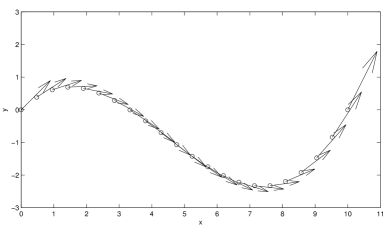
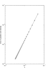
Figure 4. Left: simulation of the method (13) with $q_{0}=(0,0)$ $v_{0}=(10,10)$, $q_{N}=(10,0)$, $v_{N}=(10,20)$, $N=21$, depicting the computed points and velocities in the $xy$-plane (velocities are scaled). Right: Error in position and velocity for different values of $h$.

4.1. Variational error analysis

Now we rewrite the result of Patrick [25] and Marsden and West [21] for the particular case of a Lagrangian $L_{d}\colon TQ\times TQ\to\mathbb{R}$.

Definition 4.8.

Let $L_{d}\colon TQ\times TQ\to\mathbb{R}$ be a discrete Lagrangian. We say that $L_{d}$ is a discretization of order $r$ if there exist an open subset $U_{1}\subset T^{(2)}Q$ with compact closure and constants $C_{1}>0$, $h_{1}>0$ so that

$$|L_{d}(q(0),\dot{q}(0),q(h),\dot{q}(h),h)-L_{d}^{e}(q(0),\dot{q}(0),q(h),\dot{q}(h),h)|\leq C_{1}h^{r+1}$$

for all solutions $q(t)$ of the second-order Euler–Lagrange equations with initial conditions $(q_{0},\dot{q}_{0},\allowbreak\ddot{q}_{0})\in U_{1}$ and for all $h\leq h_{1}$.

Following [21, 26], we have the next result about the order of our variational integrator.

Theorem 4.9.

If $\widetilde{F}_{L_{d}}$ is the evolution map of an order $r$ discretization $L_{d}\colon TQ\times TQ\to\mathbb{R}$ of the exact discrete Lagrangian $L_{d}^{e}\colon TQ\times TQ\to\mathbb{R}$, then

$$\widetilde{F}_{L_{d}}=\widetilde{F}_{L_{d}^{e}}+\mathcal{O}(h^{r+1}).$$

In other words, $\widetilde{F}_{L_{d}}$ gives an integrator of order $r$ for $\widetilde{F}_{L_{d}^{e}}=F_{H}^{h}$.

Note that given a discrete Lagrangian $L_{d}\colon TQ\times TQ\to\mathbb{R}$ its order can be calculated by expanding the expressions for $L_{d}(q(0),\dot{q}(0),q(h),\dot{q}(h),h)$ in a Taylor series in $h$ and comparing this to the same expansions for the exact Lagrangian. If the series agree up to $r$ terms, then the discrete Lagrangian is of order $r$.

5. Application to optimal control of mechanical systems

In this section we will study how to apply our variational integrator to optimal control problems. We will study optimal control problems for fully actuated mechanical systems and we will show how our methods can be applied to the optimal control of a robotic leg.

In the following we will assume that all the control systems are controllable, that is, for any two points $q_{0}$ and $q_{f}$ in the configuration space $Q$, there exists an admissible control $u(t)$ defined on some interval $[0,T]$ such that the system with initial condition $q_{0}$ reaches the point $q_{f}$ at time $T$ (see [4] and [6] for example).

5.1. Optimal control of fully actuated systems.

Let $L\colon TQ\to\mathbb{R}$ be a regular Lagrangian and take local coordinates $(q^{A})$ on $Q$ where $1\leq A\leq n$. For this Lagrangian the controlled Euler–Lagrange equations are

$$\frac{d}{dt}\frac{\partial L}{\partial\dot{q}^{A}}-\frac{\partial L}{\partial q^{A}}=u_{A},$$ (18)

where $u=(u_{A})\in U\subset\mathbb{R}^{n}$ is an open subset of $\mathbb{R}^{n}$, the set of control parameters.

The optimal control problem consists in finding a trajectory of the state variables and control inputs $(q^{(A)}(t),u^{A}(t))$ satisfying (18) given initial and final conditions $(q^{A}(t_{0}),\dot{q}^{A}(t_{0}))$, $(q^{A}(t_{f}),\allowbreak\dot{q}^{A}(t_{f}))$ respectively, minimizing the cost function

$$\mathcal{A}=\int_{t_{0}}^{t_{f}}C(q^{A},\dot{q}^{A},u_{A})dt,$$

where $C\colon TQ\times U\to\mathbb{R}$.

From (18) we can rewrite the cost function as a second-order Lagrangian $\widetilde{L}\colon T^{(2)}Q\to\mathbb{R}$ given by

$$\widetilde{L}(q^{A},\dot{q}^{A},\ddot{q}^{A})=C\left(q^{A},\dot{q}^{A},\frac{d}{dt}\frac{\partial L}{\partial\dot{q}^{A}}-\frac{\partial L}{\partial q^{A}}\right)$$

replacing the controls by the Euler–Lagrange equations in the cost function (see [4] for example).

Suppose that $Q=\mathbb{R}^{n}$. Then we can define a discretization of the Lagrangian $\widetilde{L}\colon T^{(2)}Q\to\mathbb{R}$ by a discrete Lagrangian $\widetilde{L}_{d}\colon TQ\times TQ\to\mathbb{R}$,

$$\widetilde{L}_{d}(q_{k},v_{k},q_{k+1},v_{k+1}) =\frac{h}{2}\widetilde{L}\left(\frac{q_{k}+q_{k+1}}{2},\frac{v_{k}+v_{k+1}}{2},\frac{2}{h^{2}}(q_{k+1}-q_{k}-hv_{k})\right)$$

$$+\frac{h}{2}\widetilde{L}\left(\frac{q_{k}+q_{k+1}}{2},\frac{v_{k}+v_{k+1}}{2},\frac{2}{h^{2}}(q_{k}-q_{k+1}+hv_{k+1})\right).$$

In the first term, we have computed an approximate value of the acceleration $a_{k}$ by using the Taylor expansion $q_{k+1}\approx q_{k}+hv_{k}+\frac{h^{2}}{2}a_{k}$. For the second term, we have approximated $a_{k+1}$ using $q_{k}\approx q_{k+1}-hv_{k+1}+\frac{h^{2}}{2}a_{k+1}$, as in Example 3.2.

Other natural possibilities for $\widetilde{L}_{d}$ are, for instance,

$$\widetilde{L}_{d}(q_{k},v_{k},q_{k+1},v_{k+1}) =hL\left(\frac{q_{k}+q_{k+1}}{2},\frac{q_{k+1}-q_{k}}{h},\frac{v_{k+1}-v_{k}}{h}\right)$$

or

$$\widetilde{L}_{d}(q_{k},v_{k},q_{k+1},v_{k+1}) =\frac{1}{2}L\left(q_{k},v_{k},\frac{v_{k+1}-v_{k}}{h}\right)+\frac{1}{2}L\left(q_{k+1},v_{k+1},\frac{v_{k+1}-v_{k}}{h}\right).$$

Applying the results given in Section 3, we know that the minimizers of the cost function are obtained by solving the discrete second-order Euler–Lagrange equations

$$D_{1}\widetilde{L}_{d}(q_{k},v_{k},q_{k+1},v_{k+1})+D_{3}\widetilde{L}_{d}(q_{k-1},v_{k-1},q_{k},v_{k}) =0,$$

$$D_{2}\widetilde{L}_{d}(q_{k},v_{k},q_{k+1},v_{k+1})+D_{4}\widetilde{L}_{d}(q_{k-1},v_{k-1},q_{k},v_{k}) =0.$$

If the matrix

$$\left(\begin{array}[]{cc}D_{13}\widetilde{L}_{d}&D_{14}\widetilde{L}_{d}\\ D_{23}\widetilde{L}_{d}&D_{24}\widetilde{L}_{d}\\ \end{array}\right)$$

is regular, then one can define the discrete Lagrangian map to solve the optimal control problem.

Example 5.1.

Two-link manipulator

We consider the optimal control of a two-link manipulator which is a classical example studied in robotics (see for example [22] and [24]). The two-link manipulator consists of two coupled (planar) rigid bodies with mass $m_{i}$, length $l_{i}$ and moments of inertia with respect to the joints $J_{i}$, with $i=1,2$, respectively.

Figure 5. Two-link manipulator

Let $\theta_{1}$ and $\theta_{2}$ be the configuration angles measured as in Figure 5. If we assume one end of the first link to be fixed in an inertial reference frame, the configuration of the system is locally specified by the coordinates $(\theta_{1},\theta_{2})\in\mathbb{S}^{1}\times\mathbb{S}^{1}$. The Lagrangian is given by the kinetic energy of the system minus the potential energy, that is,

$$L(q,\dot{q})=\frac{1}{8}(m_{1}+4m_{2})l_{1}^{2}\dot{\theta}_{1}^{2}+\frac{1}{8}m_{2}l_{2}^{2}(\dot{\theta}_{1}+\dot{\theta}_{2})^{2}+\frac{1}{2}m_{2}l_{1}l_{2}\cos(\theta_{2})\dot{\theta}_{1}(\dot{\theta}_{1}+\dot{\theta}_{2})+\frac{1}{2}J_{1}\dot{\theta}_{1}^{2}\\ \quad+\frac{1}{2}J_{2}(\dot{\theta}_{1}+\dot{\theta}_{2})^{2}+g\left(\frac{1}{2}m_{1}l_{1}\sin\theta_{1}+m_{2}l_{1}\sin\theta_{1}+\frac{1}{2}m_{2}l_{2}(\theta_{1}+\theta_{2})\right),$$

where $g$ is the constant gravitational acceleration.

Control torques $u_{1}$ and $u_{2}$ are applied at the base of the first link and at the joint between the two links. The equations of motion of the controlled system are

$$u_{1} =-\sin\theta_{2}l_{1}l_{2}m_{2}\dot{\theta}_{2}\dot{\theta}_{1}-\frac{1}{2}\sin\theta_{2}\dot{\theta}_{2}^{2}l_{1}l_{2}m_{2}+\frac{1}{2}m_{2}l_{2}\cos(\theta_{1}+\theta_{2})g$$

$$\quad+\left(m_{2}g\cos\theta_{1}+\frac{1}{2}g\cos\theta_{1}m_{1}\right)l_{1}+\left(\frac{1}{4}m_{2}l_{2}^{2}+J_{2}+\frac{1}{2}\cos\theta_{2}l_{1}l_{2}m_{2}\right)\ddot{\theta}_{2}$$

$$\quad+\left(\cos\theta_{2}l_{1}l_{2}m_{2}+\left(\frac{m_{1}}{4}+m_{2}\right)l_{1}^{2}+\frac{m_{2}l_{2}^{2}}{4}+J_{1}+J_{2}\right)\ddot{\theta}_{1},$$

$$u_{2} =\frac{1}{2}\sin\theta_{2}l_{1}l_{2}m_{2}\dot{\theta}_{1}^{2}+\left(\frac{1}{4}m_{2}l_{2}^{2}+J_{2}+\frac{1}{2}\cos\theta_{2}l_{1}l_{2}m_{2}\right)\ddot{\theta}_{1}$$

$$\quad+\frac{1}{2}m_{2}l_{2}\cos(\theta_{1}+\theta_{2})g+\left(\frac{1}{4}m_{2}l_{2}^{2}+J_{2}\right)\ddot{\theta}_{2}.$$

We look for trajectories $(\theta_{1}(t),\theta_{2}(t),u(t))$ of the state variables and control inputs for given initial and final conditions, that is, for given values of $(\theta_{1}(0),\theta_{2}(0),\dot{\theta}_{1}(0),\dot{\theta}_{2}(0))$ and $(\theta_{1}(T),\theta_{2}(T),\allowbreak\dot{\theta}_{1}(T),\dot{\theta}_{2}(T))$, and minimizing the cost functional

$$\mathcal{A}=\frac{1}{2}\int_{0}^{T}(u_{1}^{2}+u_{2}^{2})\,dt.$$

We construct the discrete Lagrangian $\widetilde{L}_{d}\colon T(\mathbb{S}^{1}\times\mathbb{S}^{1})\times T(\mathbb{S}^{1}\times\mathbb{S}^{1})\to\mathbb{R}$, discretizing the Lagrangian $\displaystyle{\widetilde{L}\colon T^{(2)}(\mathbb{S}^{1}\times\mathbb{S}^{1})\to\mathbb{R}}$ given by

$$\widetilde{L}(\theta_{1},\theta_{2},\dot{\theta}_{1},\dot{\theta}_{2},\ddot{\theta}_{1},\ddot{\theta}_{2}) =\frac{1}{2}\left[\frac{1}{2}\sin\theta_{2}l_{1}l_{2}m_{2}\dot{\theta}_{1}^{2}+\left(\frac{1}{4}m_{2}l_{2}^{2}+J_{2}+\frac{1}{2}\cos\theta_{2}l_{1}l_{2}m_{2}\right)\ddot{\theta}_{1}\right.$$

$$\quad+\left.\frac{1}{2}m_{2}l_{2}\cos(\theta_{1}+\theta_{2})g+\left(\frac{1}{4}m_{2}l_{2}^{2}+J_{2}\right)\ddot{\theta}_{2}\right]^{2}$$

$$\quad+\frac{1}{2}\left[\frac{1}{2}\sin\theta_{2}l_{1}l_{2}m_{2}\dot{\theta}_{1}^{2}+\left(\frac{1}{4}m_{2}l_{2}^{2}+J_{2}+\frac{1}{2}\cos\theta_{2}l_{1}l_{2}m_{2}\right)\ddot{\theta}_{1}\right.$$

$$\quad+\left.\frac{1}{2}m_{2}l_{2}\cos(\theta_{1}+\theta_{2})g+\left(\frac{1}{4}m_{2}l_{2}^{2}+J_{2}\right)\ddot{\theta}_{2}\right]^{2}$$

taking the same discretization as in equation (12) to approximate the acceleration and taking midpoint averages to approximate the position and velocity.

Figures 6 and 7 show the results from a numerical simulation of the method, taking the system from the stable mechanical equilibrium $(\theta_{1}(0),\theta_{2}(0),\dot{\theta}_{1}(0),\dot{\theta}_{2}(0))=(-\pi/2,0,0,0)$ to the unstable equilibrium $(\theta_{1}(T),\theta_{2}(T),\dot{\theta}_{1}(T),\dot{\theta}_{2}(T))=(\pi/2,0,0,0)$. We have used $T=10$, $N=1000$, $m_{1}=0.375$, $m_{2}=0.25$, $l_{1}=1.5$, $l_{2}=1$, $J_{1}=\frac{m_{1}l_{1}^{2}}{3}$, $J_{2}=\frac{m_{2}l_{2}^{2}}{3}$, and $g=9.8$. In addition, the reader can find a video of the simulation in www.youtube.com/watch?v=ZUUH0596a30. The algorithm generates a sequence of velocities as well as positions, but we represent only the positions in the figures.

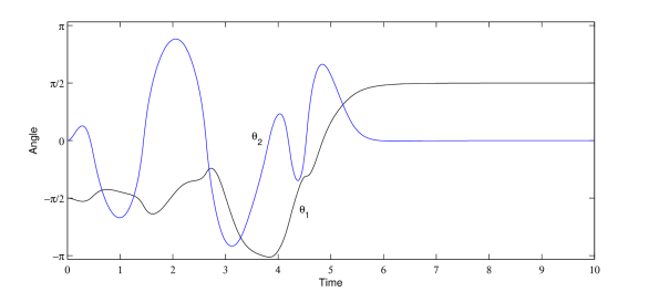
Figure 6. Angles $\theta_{1}$ and $\theta_{2}$ for the optimal control of the two-link manipulator. Initially, the two links point downwards; at $T=10$ they point upwards.

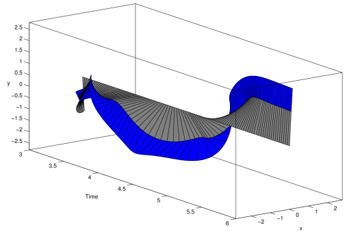
Figure 7. Evolution of the actual position of the two-link manipulator (detail for $t\in[3,6]$). Sections of this surface with the vertical plane $t=t_{0}$ show the two links as they are positioned at time $t_{0}$.

We have also considered a different setting where the angle $\theta_{2}$ is restricted to move between 0 and 170 degrees, inspired by an elbow joint. This range of motion is enforced by adding a continuous, piecewise linear function $V(\theta_{2})$ to the cost function, with slope $-1000$ for $\theta_{2}<0^{\circ}$, $0$ for $0^{\circ}<\theta_{2}<170^{\circ}$, and $1000$ for $\theta_{2}>170^{\circ}$. We simulated the optimal trajectory with the same endpoint conditions and physical parameters as above, with $N=200$. A video of the resulting motion can be found in www.youtube.com/watch?v=OxOFHdT7emQ.

Conclusions and future research

In this paper we design variational integrators for higher-order variational systems and their application to optimal control problems. The general idea for those variational integrators is to directly discretize Hamilton’s principle rather than the equations of motion in a way that preserves the original system invariants, notably the symplectic form and, via a discrete version of Noether’s theorem, the momentum map.

We show that a regular higher-order Lagrangian system has a unique solution for given nearby endpoint conditions using a direct variational proof of existence and uniqueness for the local boundary value problem using a regularization procedure assuming only $C^{k}$ differentiability (instead of $C^{2k}$ as in standard ODE theory).

We have seen that taking a discrete Lagrangian function $L_{d}\colon T^{(k-1)}Q\times T^{(k-1)}Q\to{\mathbb{R}}$ we obtain the appropriate approximation of the action $\int^{h}_{0}L(q,\dot{q},\ldots,q^{(k)})\,dt$. Moreover, we derive a particular choice of discrete Lagrangian which gives an exact correspondence between discrete and continuous systems, the exact discrete Lagrangian. We show that if the original Lagrangian is regular then it is also the exact discrete Lagrangian and how is the relation between the discrete Legendre transformations with the continuous one.

As future research, we are interested in the construction of an exact discrete Lagrangian function for higher-order mechanical systems subject to higher-order constraints. The main point will be to show the existence and uniqueness of solutions for the boundary value problem for higher-order systems subject to higher-order constraints. After it, one could define the exact discrete Lagrangian for constrained systems in a similar way that the ones shown in this work. Since optimal control problems for the class of under actuated mechanical systems can be seen as constrained higher-order variational problems, the extension of the constructions given in this work, can be useful to new developments in the field of geometric integration for optimal control problems. The case of optimal control of nonholonomic systems will be developed.

Appendix: a technical result for section 2

Let $E$ be the kernel of $g$, where $g=(g_{0},\ldots,g_{k-1})\colon C^{l}([0,1],\mathbb{R}^{n})\to(\mathbb{R}^{n})^{k}$ and $g_{j}[\cdot]=\langle b_{j}^{[k]},\cdot\rangle\kern-2.4pt\rangle$. In the context of section 2.5, $E$ is the tangent space of the constraint set defined using the linear constraints $g_{j}$, and $l$ is either $0$ or $k$.

In this Appendix we show that the orthogonal complement of $E$ is the space $F$ of $\mathbb{R}^{n}$-valued polynomials of degree at most $k-1$,

$$F=\hbox{span}_{\mathbb{R}^{n}}(b_{0}^{[k]},\ldots,b_{k-1}^{[k]})=\{c^{j}b_{j}^{[k]}|c^{0},\ldots,c^{k-1}\in\mathbb{R}^{n}\},$$

where $b_{j}^{[k]}$, $j=0,\ldots,k-1$, is a basis of the space of real-valued polynomials of degree at most $k-1$ consisting of orthonormal polynomials on $[0,1]$.

Lemma 5.2.

$F=E^{\perp}$, where the orthogonal complement is taken with respect to the inner product $\langle\kern-2.4pt\langle\cdot,\cdot\rangle\kern-2.4pt\rangle$ in $C^{l}([0,1],\mathbb{R}^{n})$.

Proof.

We will prove that $E$ and $F$ are orthogonal (with zero intersection) and that their sum is the whole space $C^{l}([0,1],\mathbb{R}^{n})$.

Let $e\in E$ and $c^{j}b_{j}^{[k]}\in F$.

$$\langle\kern-2.4pt\langle c^{j}b_{j}^{[k]},e\rangle\kern-2.4pt\rangle =\int_{0}^{1}(c^{j}b_{j}^{[k]}(u))\cdot e(u)\,du=\sum_{i=1}^{n}\int_{0}^{1}c_{i}^{j}b_{j}^{[k]}(u)e_{i}(u)du$$

$$=c^{j}\cdot\left(\int_{0}^{1}b_{j}^{[k]}(u)e_{1}(u),\ldots,\int_{0}^{1}b_{j}^{[k]}(u)e_{n}(u)\right)$$

$$=c^{j}\cdot\langle b_{j}^{[k]},e\rangle\kern-2.4pt\rangle=c^{j}\cdot g_{j}[e]=0,$$

since $e\in E=\operatorname{Ker}g$.

The fact that $E\cap F=\{0\}$ can be obtained either by using that the inner product is nondegenerate or directly as follows. Take $e\in E\cap F$, so $e=c^{j}b_{j}^{[k]}$. For all $j^{\prime}$, we have $0=g_{j^{\prime}}[e]=\langle b_{j^{\prime}}^{[k]},c^{j}b_{j}^{[k]}\rangle\kern-2.4pt\rangle=c^{j^{\prime}}$, which means that $e=0$.

Finally, take $e\in C^{l}([0,1],\mathbb{R}^{n})$. Write

$$e=e-\sum_{j=0}^{k-1}\langle b_{j}^{[k]},e\rangle\kern-2.4pt\rangle b_{j}^{[k]}+\sum_{j=0}^{k-1}\langle b_{j}^{[k]},e\rangle\kern-2.4pt\rangle b_{j}^{[k]}.$$

The third term is in $F$. The remaining part of the right-hand side is in $E$ since for all $j^{\prime}$,

$$\Big{\langle}b_{j^{\prime}},e-\sum_{j=0}^{k-1}\langle b_{j}^{[k]},e\rangle\kern-2.4pt\rangle b_{j}^{[k]}\Big{\rangle}\kern-3.59999pt\Big{\rangle}=\langle b_{j^{\prime}},e\rangle\kern-2.4pt\rangle-\sum_{j=0}^{k-1}\delta_{j^{\prime}j}\langle b_{j},e\rangle\kern-2.4pt\rangle=0.$$

Therefore $C^{l}([0,1],\mathbb{R}^{n})=E+F$. From the first part of the proof, we obtain that there is an orthogonal decomposition $C^{l}([0,1],\mathbb{R}^{n})=E\oplus F$. ∎

References

- [1] R. Abraham, J. E. Marsden and T. Ratiu, Manifolds, tensor analysis, and applications, vol. 75 of Applied Mathematical Sciences, 2nd edition, Springer-Verlag, New York, 1988, URL http://dx.doi.org/10.1007/978-1-4612-1029-0.
- [2] R. P. Agarwal, Boundary value problems for higher order differential equations, World Scientific Publishing Co., Inc., Teaneck, NJ, 1986, URL http://dx.doi.org/10.1142/0266.
- [3] R. Benito, M. de León and D. Martín de Diego, Higher-order discrete Lagrangian mechanics, Int. J. Geom. Methods Mod. Phys., 3 (2006), 421–436, URL http://dx.doi.org/10.1142/S0219887806001235.
- [4] A. M. Bloch, Nonholonomic mechanics and control, vol. 24 of Interdisciplinary Applied Mathematics, Springer-Verlag, New York, 2003, URL http://dx.doi.org/10.1007/b97376, With the collaboration of J. Baillieul, P. Crouch and J. Marsden, With scientific input from P. S. Krishnaprasad, R. M. Murray and D. Zenkov, Systems and Control.
- [5] A. M. Bloch, I. I. Hussein, M. Leok and A. K. Sanyal, Geometric structure-preserving optimal control of a rigid body, J. Dyn. Control Syst., 15 (2009), 307–330, URL http://dx.doi.org/10.1007/s10883-009-9071-2.
- [6] F. Bullo and A. D. Lewis, Geometric control of mechanical systems, vol. 49 of Texts in Applied Mathematics, Springer-Verlag, New York, 2005, URL http://dx.doi.org/10.1007/978-1-4899-7276-7, Modeling, analysis, and design for simple mechanical control systems.
- [7] C. L. Burnett, D. D. Holm and D. M. Meier, Inexact trajectory planning and inverse problems in the Hamilton-Pontryagin framework, Proc. R. Soc. Lond. Ser. A Math. Phys. Eng. Sci., 469 (2013), 20130249, 24, URL http://dx.doi.org/10.1098/rspa.2013.0249.
- [8] L. Colombo, D. Martín de Diego and M. Zuccalli, On variational integrators for optimal control of mechanical control systems, Rev. R. Acad. Cienc. Exactas Fís. Nat. Ser. A Math. RACSAM, 106 (2012), 161–171, URL http://dx.doi.org/10.1007/s13398-011-0032-8.
- [9] L. Colombo, D. Martín de Diego and M. Zuccalli, Higher-order discrete variational problems with constraints, J. Math. Phys., 54 (2013), 093507, 17, URL http://dx.doi.org/10.1063/1.4820817.
- [10] M. Crampin, W. Sarlet and F. Cantrijn, Higher-order differential equations and higher-order Lagrangian mechanics, Math. Proc. Cambridge Philos. Soc., 99 (1986), 565–587, URL http://dx.doi.org/10.1017/S0305004100064501.
- [11] P. Crouch and F. Silva Leite, The dynamic interpolation problem: on Riemannian manifolds, Lie groups, and symmetric spaces, J. Dynam. Control Systems, 1 (1995), 177–202, URL http://dx.doi.org/10.1007/BF02254638.
- [12] M. de León and P. R. Rodrigues, Generalized classical mechanics and field theory, vol. 112 of North-Holland Mathematics Studies, North-Holland Publishing Co., Amsterdam, 1985, A geometrical approach of Lagrangian and Hamiltonian formalisms involving higher order derivatives, Notes on Pure Mathematics, 102.
- [13] F. Gay-Balmaz, D. D. Holm, D. M. Meier, T. S. Ratiu and F.-X. Vialard, Invariant higher-order variational problems, Comm. Math. Phys., 309 (2012), 413–458, URL http://dx.doi.org/10.1007/s00220-011-1313-y.
- [14] F. Gay-Balmaz, D. D. Holm, D. M. Meier, T. S. Ratiu and F.-X. Vialard, Invariant higher-order variational problems II, J. Nonlinear Sci., 22 (2012), 553–597, URL http://dx.doi.org/10.1007/s00332-012-9137-2.
- [15] F. Gay-Balmaz, D. D. Holm and T. S. Ratiu, Higher order Lagrange-Poincaré and Hamilton-Poincaré reductions, Bull. Braz. Math. Soc. (N.S.), 42 (2011), 579–606, URL http://dx.doi.org/10.1007/s00574-011-0030-7.
- [16] I. I. Hussein and A. M. Bloch, Dynamic interpolation on Riemannian manifolds: an application to interferometric imaging, in Proceedings of the 2004 American Control Conference, 2004, 685–690.
- [17] B. W. Jordan and E. Polak, Theory of a class of discrete optimal control systems, J. Electronics Control (1), 17 (1964), 697–711.
- [18] T. Lee, M. Leok and N. H. McClamroch, Optimal attitude control of a rigid body using geometrically exact computations on , J. Dyn. Control Syst., 14 (2008), 465–487, URL http://dx.doi.org/10.1007/s10883-008-9047-7.
- [19] M. Leok and T. Shingel, Prolongation-collocation variational integrators, IMA J. Numer. Anal., 32 (2012), 1194–1216, URL http://dx.doi.org/10.1093/imanum/drr042.
- [20] L. Machado, F. Silva Leite and K. Krakowski, Higher-order smoothing splines versus least squares problems on Riemannian manifolds, J. Dyn. Control Syst., 16 (2010), 121–148, URL http://dx.doi.org/10.1007/s10883-010-9080-1.
- [21] J. E. Marsden and M. West, Discrete mechanics and variational integrators, Acta Numer., 10 (2001), 357–514, URL http://dx.doi.org/10.1017/S096249290100006X.
- [22] R. N. Murray, Z. X. Li and S. S. Sastry, A mathematical introduction to robotic manipulation, CRC Press, Boca Raton, FL, 1994.
- [23] L. Noakes, G. Heinzinger and B. Paden, Cubic splines on curved spaces, IMA J. Math. Control Inform., 6 (1989), 465–473, URL http://dx.doi.org/10.1093/imamci/6.4.465.
- [24] S. Ober-Blöbaum, O. Junge and J. E. Marsden, Discrete mechanics and optimal control: an analysis, ESAIM Control Optim. Calc. Var., 17 (2011), 322–352, URL http://dx.doi.org/10.1051/cocv/2010012.
- [25] G. W. Patrick, Lagrangian mechanics without ordinary differential equations, Rep. Math. Phys., 57 (2006), 437–443, URL http://dx.doi.org/10.1016/S0034-4877(06)80030-3.
- [26] G. W. Patrick and C. Cuell, Error analysis of variational integrators of unconstrained Lagrangian systems, Numer. Math., 113 (2009), 243–264, URL http://dx.doi.org/10.1007/s00211-009-0245-3.
- [27] A. P. Veselov, Integrable systems with discrete time, and difference operators, Funktsional. Anal. i Prilozhen., 22 (1988), 1–13, 96, URL http://dx.doi.org/10.1007/BF01077598.
- [28] J. M. Wendlandt and J. E. Marsden, Mechanical integrators derived from a discrete variational principle, Phys. D, 106 (1997), 223–246, URL http://dx.doi.org/10.1016/S0167-2789(97)00051-1.