Lightweight Monte Carlo Verification of Markov Decision Processes with Rewards

Abstract

Markov decision processes are useful models of concurrency optimisation problems, but are often intractable for exhaustive verification methods. Recent work has introduced lightweight approximative techniques that sample directly from scheduler space, bringing the prospect of scalable alternatives to standard numerical model checking algorithms. The focus so far has been on optimising the probability of a property, but many problems require quantitative analysis of rewards. In this work we therefore present lightweight statistical model checking algorithms to optimise the rewards of Markov decision processes. We consider the standard definitions of rewards used in model checking, introducing an auxiliary hypothesis test to accommodate reachability rewards. We demonstrate the performance of our approach on a number of standard case studies.

1 Introduction

Markov decision processes (MDP) describe systems that interleave nondeterministic actions and probabilistic transitions. Such systems may be seen as comprising probabilistic subsystems whose transitions depend on the states of the other subsystems, while the order in which concurrently enabled transitions execute is nondeterministic. This order, defined by a scheduler that is typically either history-dependent or memoryless, may radically affect the system’s behaviour. By assigning numerical rewards or costs to execution traces, MDPs have proven useful in many real optimisation problems [26]. More recently, in the context of formal verification, logics have been extended to allow model checkers to consider rewards [18].

In the classic context, rewards are assigned to actions [2, 25, 1]. In the context of model checking, rewards are often assigned to states or transitions between states [18]. In both cases the rewards are summed over the length of a trace and the expected reward is calculated by averaging the total reward with respect to the probability of the trace. In this work we focus on MDPs in the context of model checking, but the mechanism of accumulating rewards is unimportant to our algorithms and we simply assume that a total reward is assigned to a finite trace.

Figure 1 illustrates a simple MDP for which memoryless and history-dependent schedulers can give different minimum rewards for logical property $\mathbf{X}(\psi\wedge\mathbf{XG}^{4}\phi)$ (the precise semantics of this logic are defined in Section 2). Execution proceeds by first choosing an action nondeterministically, to select a distribution of probabilistic transitions, and then by making a probabilistic choice to select the next state. The property asserts that on the next step $\psi$ will be true and, on the step after that, $\phi$ will be remain true for $4$ time steps. In this example rewards $r_{0},r_{1},r_{2}$ are assigned to actions $a_{0},a_{1},a_{2}$, respectively. In the initial state ($s_{0}$) both actions $a_{1}$ and $a_{2}$ can lead to traces that satisfy the property, but subsequent actions taken in state $s_{0}$ must be $a_{1}$. If $r_{1}>r_{2}>0$, the minimum reward will be achieved by taking action $a_{2}$ in the initial state and $a_{1}$ whenever the execution visits $s_{0}$ thereafter. To satisfy the property a memoryless scheduler would be forced to always take action $a_{1}$ in state $s_{0}$ and would therefore not achieve the minimum possible reward.

Figure 1: Simple MDP with different rewards for history-dependent and memoryless schedulers.

Numerical model checking algorithms for probabilistic systems have complexity related to the number of states of the model and therefore scale exponentially with the number of interacting variables [3]. Numerical algorithms to find optimal schedulers in MDPs incur the additional costs of optimisation [18]. Statistical model checking (SMC) describes a collection of Monte Carlo techniques that approximate the results of numerical model checking and aim not to construct an explicit representation of the state space—states are generated on the fly during simulation. While memory-efficient (“lightweight”) SMC techniques have been developed to address the probabilistic model checking problem, until recently [22] it has not been possible to address the nondeterministic problem in this way. In addition to not incurring the cost of exploring the state space, a significant advantage of lightweight SMC approaches is that they may be efficiently distributed on memory-sensitive high performance parallel computing architectures, such as GPGPU (general purpose computing on graphics processing units).

SMC makes use of an executable model, so to apply SMC to MDPs the nondeterminism must be resolved by a scheduler. Since nondeterministic and probabilistic choices are interleaved in an MDP, memoryless schedulers are typically of the same order of complexity as the system as a whole and may be infinite. History-dependent schedulers are exponentially bigger. The key contribution of [22] is the introduction of techniques to define the behaviour of schedulers in $\mathcal{O}(1)$ memory, allowing them to be sampled at random and tested individually. These techniques offer a significant saving in computation over enumeration, with performance effectively independent of the size of the sample space and only dependent on the relative abundance of ‘near-optimal’ [16] schedulers.

The basic idea of [22] is to select a number of schedulers at random and apply SMC to each of the discrete time Markov chains they induce. In this way it is possible to estimate or test hypotheses about the maximum and minimum probabilities of a property. The simple sampling strategies of [22] have been significantly enhanced by so-called “smart sampling” in [9]. Smart sampling makes gains in performance by refining a candidate set of schedulers and not wasting simulation budget on those that are obviously sub-optimal.

In this work we present algorithms to find schedulers that approximately maximise or minimise the expected reward of finite traces in Markov decision processes. Our algorithms are based on the elemental sampling strategies given in [22] and the smart sampling techniques of [9]. The passage from probabilities to rewards is intuitive, but not immediate, due to the specific way rewards are defined in the context of model checking [18] and to the fact that the values of rewards are arbitrary. Unlike probabilities, rewards have no inherent a priori bounds, so the standard statistical techniques to bound the absolute error do not apply. Our solution is to use a relative bound, based on a generalisation of the standard Chernoff-Hoeffding bound used in SMC. A further challenge is that the commonly used ‘reachability rewards’ [18] assume the probability of a property is known with absolute certainty and, somewhat arbitrarily, define the reward of properties with probability less than $1$ to be infinite. With no a priori information about the property, this definition induces an unknown distribution with potentially infinite variance. As such, its properties cannot be directly estimated by sampling. Our solution is to introduce an auxiliary hypothesis test to assert that the probability of the property is $1$. The estimation results can then be said to lie within the specified confidence bounds given that the hypothesis is true, while the confidence of the hypothesis test can be made arbitrarily high.

We have implemented the algorithms in our statistical model checking platform, Plasma [15, 5], and have applied them to a number of case studies from the literature. The results demonstrate that our approach is highly effective on many models and produces useful bounds when near-optimal schedulers are rare.

Related Work

The exponential scaling of numerical algorithms, such as policy iteration and value iteration [2, 25], has prompted much work on sampling techniques to approximately optimise discounted rewards over infinite horizons (see, e.g., [7] for a survey). Of this work, the Kearns algorithm [16] is relevant to the present context because it is lightweight in concept and used by [21] in the context of SMC. To find the action with the greatest expected reward in the current state, the algorithm recursively estimates the rewards of successive states using sampling, until successive estimates differ by less than some user-defined threshold.

The rewards used in model checking are typically not discounted and defined over finite horizons [18]. There is much less work on approximative techniques for the finite horizon problem in the classic literature. Below we summarise several recent attempts to apply SMC to MDPs [4, 21, 11, 10, 22, 6, 9], although none of these address the standard model checking problems of MDPs with rewards.

In [4, 10] the authors present algorithms to remove ‘spurious’ nondeterminism on the fly, so that standard SMC may be used. This approach is limited to the class of MDPs whose nondeterminism is not affected by scheduling.

In [11] the authors count the occurrence of state-actions in simulations, to iteratively improve a probabilistic scheduler that is assessed using sequential hypothesis testing. If an example is found it is correct, but the frequency of state-actions is not in general indicative of global optimality.

In [21] the authors use an adaptation of the Kearns algorithm to find a memoryless scheduler that is near optimal with respect to a discounted reward scheme. The resulting scheduler induces a Markov chain whose properties may be verified with standard SMC. Such properties are only indirectly related to the original MDP.

In [6] the authors present learning algorithms to bound the maximum probability of (unbounded) reachability properties. The algorithms refine upper and lower bounds associated to individual state-actions, according to the contribution of individual simulations. The algorithms converge very slowly and may not converge to the global optimum for similar reasons to those affecting [11].

The above SMC approaches use data structures whose size scales with the state space of the MDP. In [22] the authors introduce lightweight techniques to sample directly from scheduler space using constant memory. The simple sampling strategies of [22] are made more efficient in [9]. The present work builds on the results of [22] and [9], which are reviewed in Section 3.

2 Preliminaries

In this work an MDP comprises a possibly infinite set of states $S$, a finite set of actions $A$, a finite set of probabilities $Q$ and a relation $T:S\times A\times S\times Q$, such that $\forall s\in S$ and $\forall a\in A$, $\sum_{\forall s^{\prime}\in S}T(s,a,s^{\prime})=r$, where $r\in\{0,1\}$. The execution of an MDP proceeds by a sequence of transitions between states, starting from an initial state, inducing a set of possible traces $\Omega=S^{+}$. Given an MDP in state $s$, an action $a$ is chosen nondeterministically from the set $\{a^{\prime}\in A:\sum_{\forall s^{\prime}\in S}T(s,a^{\prime},s^{\prime})=1\}$. A new state $d\in S$ is then chosen at random with probability $T(s,a,d)$. We assume that rewards are defined by some function $R:S^{+}\rightarrow\mathbb{Q}$ or $R:A^{+}\rightarrow\mathbb{Q}$ that maps a sequence of states or a sequence of actions to a total reward. In what follows we abuse the notation and simply write $R(\omega)$ to mean the total reward assigned to trace $\omega\in\Omega$ according to an arbitrary reward scheme.

We later present algorithms to find deterministic schedulers that approximately maximise or minimise expected rewards for an MDP. A history-dependent scheduler is a function $\mathfrak{S}:\Omega\rightarrow A$. A memoryless scheduler is a function $\mathfrak{M}:S\rightarrow A$. Intuitively, at each state in the course of an execution, a history-dependent scheduler chooses an action based on the sequence of previous states and a memoryless scheduler chooses an action based only on the current state. History-dependent schedulers therefore include memoryless schedulers. In the context of SMC we consider finite simulation traces of bounded length, hence $\mathfrak{S}$ and $\mathfrak{M}$ are finite.

In this work we assume properties are defined in a bounded linear time temporal logic with the following syntax:

$$\phi=\phi\vee\phi\mid\phi\wedge\phi\mid\neg\phi\mid\mathbf{X}\phi\mid\mathbf{F}^{k}\phi\mid\mathbf{G}^{k}\phi\mid\phi\mathbf{U}^{k}\phi\mid\alpha$$ (1)

The symbol $\alpha$ denotes an atomic property that is either true or false in a state. Given a trace $\omega\in\Omega$, comprising states $s_{0}s_{1}\dots$, $\omega^{(i)}$ denotes the trace suffix $s_{i}s_{i+1}\dots$. The satisfaction relation $\models$ over (1) is constructed inductively as follows:

$$\begin{split}\omega^{(i)}\models\,&true\\ \omega^{(i)}\models\,&\alpha\iff\alpha\textnormal{ is }\mathit{true}\textnormal{ in state }\omega_{i}\\ \omega^{(i)}\models\,&\neg\varphi\iff\omega^{(i)}\models\varphi\not\in\,\models\\ \omega^{(i)}\models\,&\varphi_{1}\vee\varphi_{2}\iff\omega^{(i)}\models\varphi_{1}\textnormal{ or }\omega^{(i)}\models\varphi_{2}\\ \omega^{(i)}\models\,&\mathbf{X}^{k}\varphi\iff\omega^{(k+i)}\models\varphi\\ \omega^{(i)}\models\,&\varphi_{1}\mathbf{U}^{k}\varphi_{2}\iff\exists j\in\{i,\dots,i+k\}:\omega^{(j)}\models\varphi_{2}\\ &\wedge(j=i\vee\forall l\in\{i,\dots,j-1\}:\omega^{(l)}\models\varphi_{1})\end{split}$$ (2)

Other elements of the relation are constructed using the equivalences $\mathit{false}\equiv\neg\mathit{true}$, $\phi\wedge\phi\equiv\neg(\neg\phi\vee\neg\phi)$, $\mathbf{F}^{k}\phi\equiv\mathit{true}\mathbf{U}^{k}\phi$, $\mathbf{G}^{k}\phi\equiv\neg(\mathit{true}\mathbf{U}^{k}\neg\phi)$.

SMC algorithms typically work by constructing an automaton to decide the truth of the statement $\omega\models\varphi$, i.e., whether simulation trace $\omega$ satisfies property $\varphi$. The expected probability of $\varphi$ is then estimated by $\frac{1}{N}\sum_{i=1}^{N}\mathbf{1}(\omega_{i}\models\varphi)$, where $\omega_{1},\dots,\omega_{N}$ are $N$ statistically independent random simulation traces and $\mathbf{1}:\{\mathit{true},\mathit{false}\}\rightarrow\{0,1\}$ is an indicator function that returns $1$ if its argument is true and $0$ otherwise. To bound the estimation error it is common to use the “Chernoff” bound of [24]. The user specifies an absolute error $\varepsilon$ and a probability $\delta$ to define the bound $\mathrm{P}(\mid\hat{p}-p\mid\geq\varepsilon)\leq\delta$, where $p$ and $\hat{p}$ are respectively the true probability and the estimated probability. The bound is guaranteed if the number of simulations $N$ satisfies the relation

$$N\geq\left\lceil(\ln 2-\ln\delta)/(2\varepsilon^{2})\right\rceil.$$ (3)

3 Lightweight Verification with Smart Sampling

We recall here the techniques of lightweight verification presented in [22] and [9].

3.1 Pseudo-Random Number Generators

To avoid storing schedulers as explicit mappings, we construct schedulers on the fly using uniform pseudo-random number generators (PRNG) that are initialised by a seed and iterated to generate the next pseudo-random value. Our technique uses two independent PRNGs that respectively resolve probabilistic and nondeterministic choices. The first is used in the conventional way to make pseudo-random choices during a simulation experiment. The second PRNG is used to choose actions such that the choices are consistent between different simulations in the same experiment. Given multiple simulation experiments, the further role of the second PRNG is to range uniformly over all possible sets of choices. The seed of the second PRNG can be seen as the identifier of a specific scheduler.

To estimate the probability of a property under a scheduler, we generate multiple probabilistic simulation traces by fixing the seed of the PRNG for nondeterministic choices while choosing random seeds for the PRNG for probabilistic choices. To ensure that we sample from history-dependent schedulers, we construct a per-step PRNG seed that is a hash of a large integer representing the sequence of states up to the present and a specific scheduler identifier [22].

3.2 Hashing the Trace

We assume that the state of an MDP is an assignment of values to a vector of $n$ system variables $v_{i},i\in\{1,\dots,n\}$, with each $v_{i}$ represented by a number of bits $b_{i}$. The state can thus be represented by the concatenation of the bits of the system variables, while a sequence of states (a trace) may be represented by the concatenation of the bits of all the states. We interpret such a sequence of states as an integer of $\sum_{i=1}^{n}b_{i}$ bits, denoted $\overline{s}$, and refer to this as the trace vector. A scheduler is denoted by an integer $\sigma$ of $b_{\sigma}$ bits, which is concatenated to $\overline{s}$ (denoted $\sigma:\overline{s}$) to uniquely identify a trace and a scheduler. Our approach is to generate a hash code $h=\mathcal{H}(\sigma:\overline{s})$ and to use $h$ as the seed of a PRNG that resolves the next nondeterministic choice. In this way we can approximate the scheduler functions $\mathfrak{S}$ and $\mathfrak{M}$: $\mathcal{H}$ maps $\sigma:\overline{s}$ to a seed that is deterministically dependent on the trace and the scheduler; the PRNG maps the seed to a value that is uniformly distributed but also deterministically dependent on the trace and the scheduler. Algorithm 1 implements these ideas as a simulation function that returns a trace, given a scheduler and bounded temporal property as input. The uniformity of scheduler selection is demonstrated by the accuracy of the estimates labelled ‘uniform prob.’ in Fig. 4.

Input:

$\mathcal{M}$: an MDP with initial state $s_{0}$

$\varphi$: a bounded temporal logic property

$\sigma$: an integer identifying a scheduler

Output:

$\omega$: a simulation trace

1

2Let $\mathcal{U}_{\mathrm{prob}},\mathcal{U}_{\mathrm{nondet}}$ be uniform PRNGs with respective samples $r_{\mathrm{pr}},r_{\mathrm{\mathrm{nd}}}$

3Let $\mathcal{H}$ be a hash function

4Let $s$ denote a state, initialised $s\leftarrow s_{0}$

5Let $\omega$ denote a trace, initialised $\omega\leftarrow s$

6Let $\overline{s}$ be the trace vector, initially empty

7Select seed of $\mathcal{U}_{\mathrm{prob}}$ randomly

8while $\omega\models\varphi$ is not decided do

9      

10      $\overline{s}\leftarrow\overline{s}:s$

11      Set seed of $\mathcal{U}_{\mathrm{nondet}}$ to $\mathcal{H}(\sigma:\overline{s})$

12      Iterate $\mathcal{U}_{\mathrm{nondet}}$ to generate $r_{\mathrm{nd}}$ and use to resolve nondeterministic choice

13      Iterate $\mathcal{U}_{\mathrm{prob}}$ to generate $r_{\mathrm{pr}}$ and use to resolve probabilistic choice

14      Set $s$ to the next state

15      $\omega\leftarrow\omega:s$

16

Algorithm 1 Simulate

3.3 Implementation

To implement our approach we use an efficient hash function that constructs seeds incrementally using standard precision mathematical operations. The function is based on modular division [17, Ch. 6], such that $h=(\sigma:\overline{s})\bmod m$, where $m$ is a large prime not close to a power of 2 [8, Ch. 11]. Since $\overline{s}$ is typically very large, we use Horner’s method [13][17, Ch. 4] to generate $h$: we set $h_{0}=\sigma$ and find $h\equiv h_{n}$ ($n$ as above) by iterating the recurrence relation

$$h_{i}=(h_{i-1}2^{b_{i}}+v_{i})\bmod m.$$ (4)

Equation (4) allows us to generate a hash code knowing only the current state and the hash code from the previous step. When considering memoryless schedulers we need only know the current state. Using suitable congruences [22], the following equation allows (4) to be implemented using efficient native arithmetic:

$$(h_{i-1}2^{j})\bmod m=(h_{i-1}2^{j-1})\bmod m+(h_{i-1}2^{j-1})\bmod m$$

In a typical implementation on current hardware, a hash function and PRNG may span around $10^{19}$ schedulers. This is usually many orders of magnitude more than the number of schedulers sampled. There is no advantage in sampling from a larger set of schedulers until the number of samples drawn approaches the size of the sample space.

3.4 Multiple Estimates

To avoid the cumulative error when choosing a single probability estimate from a number of alternatives, [22] defines the following Chernoff bound for multiple estimates:

$$N\geq\left\lceil\left(\ln 2-\ln\left(1-\sqrt[M]{1-\delta}\right)\right)/(2\varepsilon^{2})\right\rceil.$$ (5)

Given $M$ estimates $\{\hat{p}_{1},\dots,\hat{p}_{M}\}$ of corresponding true probabilities $\{p_{1},\dots$, $p_{M}\}$ each generated with $N$ samples, (5) asserts that for any estimate $\hat{p}_{i}$, in particular the minimum or maximum, $\mathrm{P}(\mid\hat{p}_{i}-p_{i}\mid\geq\varepsilon)\leq\delta$. Note that when $M=1$, (5) degenerates to (3).

3.5 Smart Sampling

The elemental sampling strategies presented in [22] have the disadvantage that they allocate equal simulation budget to all schedulers, regardless of their merit. Intuitively, the performance of a scheduler may become apparent, if not certain, long before all its simulation budget has been used. The idea of smart sampling is to not waste budget on schedulers that are clearly not optimal, to thus maximise the probability of finding an optimal scheduler with a finite simulation budget. We recall here the basic notions of smart sampling introduced in [9].

In general, the problem of finding optimal schedulers using sampling has two independent components: the rarity of near-optimal schedulers (denoted $p_{g}$) and the average probability of the property under near-optimal schedulers (denoted $p_{\overline{g}}$). A near-optimal scheduler is one whose reward or probability (depending on the context) is within some $\varepsilon$ of the optimal value. If we select $M$ schedulers at random, using the techniques presented above, and verify each with $N$ simulations, the expected number of traces that satisfy the property using a near-optimal scheduler is thus $Mp_{g}Np_{\overline{g}}$ . The probability of seeing a trace that satisfies the property using a near-optimal scheduler is the cumulative probability

$$(1-(1-p_{g})^{M})(1-(1-p_{\overline{g}})^{N}).$$ (6)

To maximise the chance of seeing a good scheduler with a simulation budget of $N_{\max}=NM$, $N$ and $M$ should be chosen to maximise (6). Then, following a sampling experiment using these values, any scheduler that produces at least one trace that satisfies $\varphi$ becomes a candidate for further investigation. Since the values of of $p_{g}$ and $p_{\overline{g}}$ are unknown a priori, it is necessary to perform an initial uninformed sampling experiment to estimate them, setting $N=M=\lceil\sqrt{N_{\max}}\rceil$. The results can be used to numerically optimise (6), however an effective heuristic is to set $N=\lceil 1/\hat{p}_{\overline{g}}\rceil$, where $\hat{p}_{\overline{g}}$ is the maximum observed estimate (or minimum non-zero estimate in the case of finding minimising schedulers).

The best scheduler is found by iteratively refining the candidate set. At each iteration the per-iteration simulation budget ($N_{\max}$) is divided between the remaining candidates, simulations are performed and the average reward for each scheduler is estimated. Schedulers whose estimates fall into the “worst” quantile (lower or upper half, depending on context) are discarded. Refinement continues until estimates are known with specified confidence, according to (5). With a per-iteration budget satisfying (3), the algorithm is guaranteed to terminate with a valid estimate.

4 Statistical Model Checking with Rewards

The notions of probability estimation used in standard SMC can be adapted to estimate the expected reward of a trace. Given a function $R(\omega)\in[a,b]$, $a,b$ finite, that assigns a total reward to simulation trace $\omega$, the expected reward may be estimated by $\frac{1}{N}\sum_{i=1}^{N}R(\omega_{i})$, where $\omega_{1},\dots,\omega_{N}$ are statistically independent simulation traces. Since rewards may take values outside $[0,1]$, we must use Hoeffding’s generalisation of (3) to bound the errors [12]. To guarantee $\mathrm{P}(\mid\hat{r}-r\mid\geq\varepsilon)\leq\delta$, where $r$ and $\hat{r}$ are respectively the true and estimated values of expected reward, $N$ is required to satisfy the relation

$$N\geq\left\lceil\ln(2/\delta)\times(a-b)^{2}/(2\varepsilon^{2})\right\rceil.$$ (7)

For non-trivial problems the values of $a$ and $b$ are usually not known, while guaranteed a priori bounds (e.g., by assuming maximum or minimum possible rewards on each step) may be too conservative to be useful. While it is possible to develop a strategy using a posteriori estimates of $a$ and $b$, i.e., based on $\max_{i\in\{1,\dots,N\}}(R(\omega_{i}))$ and $\min_{i\in\{1,\dots,N\}}(R(\omega_{i}))$, we see that $N$ depends on the ratio of the absolute error $\varepsilon$ to the range of values $(a-b)$. The confidence of estimates of rewards may therefore be specified a priori as a percentage of the maximum range of the support of $R$. We adopt this idea in Algorithm 2, where we use (3) and (5) and assume that $\varepsilon$ expresses a percentage as a fraction of $1$.

Rewards Properties

The rewards properties commonly used in numerical model checking are based on an extension of the logic PCTL [18]. This extension defines instantaneous rewards (the average reward assigned to the $k^{\mathrm{th}}$ state of all traces, denoted $\mathbf{I}^{k}$), cumulative rewards (the average total reward accumulated up to the $k^{\mathrm{th}}$ state of all traces, denoted $\mathbf{C}^{k}$) and reachability rewards (the average accumulated reward of traces that eventually satisfy property $\varphi$, denoted $\mathbf{F}\varphi$). Instantaneous and cumulative rewards are based on finite traces and can be immediately approximated by sampling, using (3) and (5) to bound the errors. Reachability rewards are based on unbounded $\mathbf{F}$ and require additional consideration.

By the definition of reachability rewards [18], properties that are not satisfied with probability $1$ are assigned infinite reward. The rationale behind this is that if $\mathrm{P}(\mathbf{F}\varphi)<1$, there must exist an infinite path that does not satisfy $\varphi$, whose rewards will accumulate infinitely. This definition is somewhat arbitrary, since rewards are not constrained to be positive—an infinite sum of positive and negative values can equate to zero—and it is also possible for an infinite sum of positive values to converge, as in the case of discounted rewards.

The definition of reachability rewards makes sense in the context of numerical model checking, where paths are not considered explicitly and unbounded properties can be quantified with certainty, but it causes problems for sampling. In particular, using sampling alone it is not possible to say with certainty whether $\mathrm{P}(\mathbf{F}\varphi)=1$, even if every observed trace of finitely many satisfies $\varphi$. Without additional guarantees, the random variable from which samples are drawn could include the value infinity, giving it infinite variance. Statistical error bounds, which generally rely on an underlying assumption of finite variance, will therefore not be correct without additional measures.

To accommodate the standard definition of reachability rewards, our solution is to implement $\mathbf{F}\varphi$ as $\mathbf{F}^{k}\varphi$, i.e., bounded reachability, with an auxiliary hypothesis test to assert that $\mathrm{P}(\mathbf{F}\varphi)=1$ is true. A positive result is thus an estimate within user-specified confidence plus an accepted hypothesis within other user-specified confidence. A negative result is a similar estimate, but with an hypothesis that is not accepted. This approach is consistent with intuition and with the SMC ethos to provide results within statistical confidence bounds. The hypothesis test may be implemented in any number of standard ways. Our implementation uses a convenient normal approximation model, which we describe in Section 5.

In practice, the bound $k$ for reachability rewards is set much longer than it is supposed necessary to satisfy $\varphi$ and the hypothesis is of the form $\mathrm{P}(\mathbf{F}^{k}\varphi)\geq p_{0}$, $p_{0}\lessapprox 1$. Intuitively, the more traces of length $\leq k$ that satisfy $\varphi$, the more confident we are that $\mathrm{P}(\mathbf{F}\varphi)\geq p_{0}$ is true. Traces that fail to satisfy $\varphi$ after $k$ steps may nevertheless satisfy $\varphi$ if allowed to continue, hence the value of $p_{0}$ defines how certain we wish to be after $k$ steps. If the hypothesis is rejected, we may either conclude that the average reward is infinite (by definition), accept the calculated average reward as a lower bound or increase $k$ and try again.

Our SMC engine quits as soon as a property is satisfied or falsified, so there is very little penalty in setting $k$ large when we require high confidence, i.e., when $p_{0}\approx 1$. Simulations that satisfy the property will take only as long as necessary, independent of $k$, while those that do not satisfy the property will be few because the auxiliary hypothesis is falsified quickly when $p_{0}$ is close to 1.

Finding schedulers that optimise the rewards defined in [18] has a conceptual advantage over finding schedulers that optimise the probability of a property. This is because the effective probability of these rewards properties is always close to $1$. In the case of instantaneous and cumulative rewards, traces are not filtered with respect to a property, so the probability of acceptance is $1$. In the case of reachability rewards, either nearly all traces satisfy the property (‘nearly’ because the auxiliary hypothesis test allows for the case that not all traces satisfy the property) or the reward is assumed to be infinite. Hence, the case of probabilities significantly less than $1$ does not have to be quantified, just detected. The consequence of this, according to (6), is that the simulation budget to generate the initial candidate set can be allocated entirely to schedulers, i.e., $N=1$ and $M=N_{\max}$.

5 Smart Reward Estimation Algorithm

Algorithm 2 finds schedulers that maximise rewards. The algorithm to minimise rewards follows intuitively: replace instances of ‘$\max$’ with ‘$\min$’ in lines 2, 2, 2 and the Output line, and replace line 2 with $S\leftarrow\{\sigma\in S\mid\sigma=Q^{\prime}(n)\wedge n\in\{1,\dots,\lceil|S|/2\rceil\}\}$.

The reward property $\rho$ may be of type instantaneous, cumulative or reachability, which are denoted $\mathbf{I}^{k}\varphi$, $\mathbf{C}^{k}\varphi$ and $\mathbf{F}^{k}\varphi$, respectively, to unify the description. The reward function $\mathcal{R}_{\rho}:\mathbb{N}\times\Omega\rightarrow\mathbb{Q}$ maps the identifier of a scheduler and a trace to a reward, given reward property $\rho$. In the case of $\mathbf{I}^{k}\varphi$ and $\mathbf{C}^{k}\varphi$, $k$ is the standard user-specified parameter for these rewards and $\varphi$ is implicitly $\mathbf{G}^{k}\mathit{true}$. In the case of $\mathbf{F}^{k}\varphi$, $\varphi$ is user-specified and $k$ is set as large as feasible to satisfy the hypothesis $\mathrm{P}(\mathbf{F}^{k}\varphi)\geq p_{0}$, with confidence defined by $\alpha$ (described below). Given that our actual requirement is that $\mathrm{P}(\mathbf{F}\varphi)=1$, both $p_{0}$ and $\alpha$ will typically be close to $1$, such that very few traces will be necessary to falsify the hypothesis.

Input:

$\mathcal{M}$: an MDP

$\rho\in\{\mathbf{I}^{k}\varphi,\mathbf{C}^{k}\varphi,\mathbf{F}^{k}\varphi\}$: a reward property

$\mathcal{R}_{\rho}$: the reward function for $\rho$

$H_{0}:\mathrm{P}(\mathbf{F}^{k}\varphi)\geq p_{0}$: the auxiliary hypothesis

$z(\alpha)$: confidence of $H_{0}$, the normal quantile of order $\alpha$

$\varepsilon,\delta$: the reward estimation Chernoff bound

$N_{\max}>\ln(2/\delta)/(2\varepsilon^{2})$: the per-iteration budget

Output:

$\hat{r}_{\overline{\max}}\approx r_{\max}$, where $r_{\overline{\max}}\approx r_{\max}$ and $\mathrm{P}(|r_{\overline{\max}}-\hat{r}_{\overline{\max}}|\geq\varepsilon)\leq\delta$

1

2$N\leftarrow 1,\,M\leftarrow N_{\max}$

3$S\leftarrow\{M\textnormal{ seeds chosen uniformly at random}\}$

4$\forall\sigma\in S,\forall j\in\{1,\dots,N\}:\omega_{j}^{\sigma}\leftarrow\mathrm{Simulate}(\mathcal{M},\varphi,\sigma)$

5$Q\leftarrow\{(\sigma,q)\mid\sigma\in S\wedge\mathbb{Q}\ni q=\sum_{j=1}^{N}\mathcal{R}_{\rho}(\sigma,\omega_{j}^{\sigma})/N\}$

6$\forall\sigma\in S:\;\mathit{trues}(\sigma)\leftarrow 0$

7$\mathit{samples}\leftarrow 0,\,\mathit{conf}\leftarrow 1,\,i\leftarrow 0$

8

9while $\mathit{conf}>\delta\wedge S\neq\emptyset$ do

10      

11      $i\leftarrow i+1$

12      $M_{i}\leftarrow|S|,\,N_{i}\leftarrow 0$

13      while $\mathit{conf}>\delta\wedge N_{i}<\lceil N_{\max}/M_{i}\rceil$ do

14            

15            $N_{i}\leftarrow N_{i}+1$

16            $\mathit{conf}\leftarrow 1-(1-e^{-2\epsilon^{2}N_{i}})^{M_{i}}$

17            $\forall\sigma\in S:\;\omega_{N_{i}}^{\sigma}\leftarrow\mathrm{Simulate}(\mathcal{M},\varphi,\sigma)$

18            $\mathit{samples}\leftarrow\mathit{samples}+1$

19      

20      $Q\leftarrow\{(\sigma,q)\mid\sigma\in S\wedge\mathbb{Q}\ni q=\sum_{j=1}^{N_{i}}\mathcal{R}_{\rho}(\sigma,\omega_{j}^{\sigma})/N_{i}\}$

21      $\sigma_{\max}\leftarrow\mathop{\arg\max}_{\sigma\in S}\,Q(\sigma)$

22      $\hat{r}_{\overline{\max}}\leftarrow Q(\sigma_{\max})$

23      $\forall\sigma\in S,j\in\{1,\dots,N_{i}\}:\;\mathit{trues}(\sigma)=\mathit{trues}(\sigma)+\mathbf{1}(\omega_{j}^{\sigma}\models\varphi)$

24      $Q^{\prime}:\{1,\dots,|S|\}\rightarrow S$ is an injective function s.t.

       $\forall(n,\sigma),(n^{\prime},\sigma^{\prime})\in Q^{\prime}:\;n>n^{\prime}\implies Q(\sigma)\geq Q(\sigma^{\prime})$

25      $S\leftarrow\{\sigma\in S\mid\sigma=Q^{\prime}(n)\wedge n\in\{\lfloor|S|/2\rfloor,\dots,|S|\}\}$

26

27$Z\leftarrow(\mathit{trues}(\sigma_{\max})-\mathit{samples}\times p_{0})/\sqrt{\mathit{samples}\times p_{0}\,(1-p_{0})}$

28if $Z\leq z(\alpha)$ then

29      $H_{0}$ is rejected

30

Algorithm 2 Reward Estimation

The initial candidate set of schedulers and corresponding estimates are generated in lines 2 to 2. Applying (6), $1$ simulation is performed using each of $N_{\max}$ schedulers chosen at random. The function $Q$ maps schedulers to their current estimate. A number of initialisations take place in lines 2 to 2.

The function $\mathit{trues}$ is used by the auxiliary hypothesis test and counts the total number of traces per scheduler that satisfy the property. The variable $\mathit{samples}$ is also used by the auxiliary hypothesis test and counts the total number of traces used by any scheduler. The value of $\mathit{conf}$, initialised to $1$ to ensure at least one iteration, is the probability that the estimates exceed their specified bounds (defined by $\varepsilon$), given the current number of simulations. The main loop (lines 2 to 2) terminates when $\mathit{conf}$ is less than or equal to the specified probability $\delta$. Typically, the per-iteration budget will be such that the required confidence is reached according to (5) before the candidate set is reduced to a single element. Lines 2 to 2 contain the main simulation loop, which quits as soon as the required confidence is reached. Lines 2 to 2 order the results by estimated reward and select the upper quantile of schedulers.

The auxiliary hypothesis test necessary for reachability rewards is provided in lines 2 to 2. To test $\mathrm{P}(\mathbf{F}^{k}\varphi)\geq p_{0}$, it considers the error statistic $Z=\mathit{samples}\times(\hat{p}_{\varphi}-p_{0})/\sqrt{\mathit{samples}\times p_{0}(1-p_{0})}$, where $\hat{p}_{\varphi}=\mathit{trues}(\sigma_{\max})/\mathit{samples}$ is the estimate of $\mathrm{P}(\mathbf{F}^{k}\varphi)$. For typical values of $\mathit{samples}$, the distribution of $Z$ is well approximated by a normal with mean $=0$ and variance $=1$ when the expectation of $\hat{p}_{\varphi}$, denoted $\mathrm{E}(\hat{p}_{\varphi})$, is equal to $p_{0}$. To test the hypothesis with confidence $\alpha$, the algorithm compares the statistic $Z$ with the standard normal quantile of order $\alpha$, denoted $z(\alpha)$. The value of $z(\alpha)$ may be drawn from a table or approximated numerically. If $\mathrm{E}(\hat{p}_{\varphi})\geq p_{0}$, the value of $Z$ will be $\geq z(\alpha)$ with probability $\geq\alpha$.

To simplify the presentation of our algorithm, the auxiliary hypothesis test is also used by the instantaneous and cumulative rewards. In these latter cases, however, the test is guaranteed to be satisfied. Also for the sake of simplicity, the algorithm assumes that all simulation traces reach the $k^{\mathrm{th}}$ state without halting.

6 Case Studies

We have implemented Algorithms 1 and 2 in our statistical model checking platform, Plasma${}^{\ref{fn:plasma}}$, and take advantage of its distributed verification algorithm on the Igrida parallel computational grid. All timings are based on 64 simulation cores. The following results demonstrate typical performance on a selection of standard case studies, including one with intractable state space. We necessarily use models whose expected rewards can be calculated or inferred using numerical methods, but observe that this does not give our algorithms any advantage. The models and properties can be found on our website${}^{\ref{fn:plasma}}$ and are illustrated in detail on the Prism case studies website.

In most instances we were able to achieve accurate results with a relatively modest per-iteration simulation budget of $N_{\max}=10^{5}$ simulations, using a Chernoff bound of $\varepsilon=\delta=0.01$. In the case of the gossip protocol (Section 6.3), this budget was apparently not sufficient for all considered parameters. We nevertheless claim that the results provide useful conservative bounds. Note that for all reachability rewards we made the value of $k$ in the auxiliary hypothesis test sufficiently large to ensure that all traces satisfied the property, giving us maximum confidence for the specified budget.

6.1 Network Virus Infection

Our network virus infection case study is based on [20] and initially comprises the following sets of linked nodes: a set containing one node infected by a virus, a set with no infected nodes and a set of uninfected barrier nodes which divides the first two sets. A virus chooses which node to infect nondeterministically. A node detects a virus probabilistically and we vary this probability as a parameter for barrier nodes. Figure 3 illustrates the results of using a reachability reward property to estimate the maximum and minimum expected number of detected attacks before a particular node is infected. Each point required approximately 15 seconds of simulation time. The solid lines indicate values calculated numerically. All estimates are within $\pm 1\%$ of the true values.

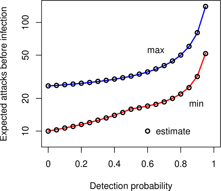
Figure 2: Network virus infection.

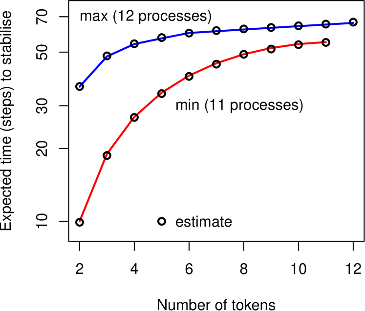
Figure 3: Self-stabilising protocol.

6.2 Self Stabilisation

The self-stabilising protocol of [14] works asynchronously to ensure that a number of networked processes share a single ‘privileged status’ token fairly. The protocol is designed to reach this dynamical state even if initially there are several tokens in the ring. For various numbers of processes, we used reachability properties to estimate the maximum and minimum expected number of steps to reach stability, given different initial numbers of tokens. Figure 3 plots typical results: the maximum values for 12 processes and the minimum values for 11 processes. Individual estimates required between 1 and 3 minutes of simulation time. The solid lines indicate values calculated numerically. All estimates are within $\pm 1\%$ of the true values.

6.3 Gossip Protocol

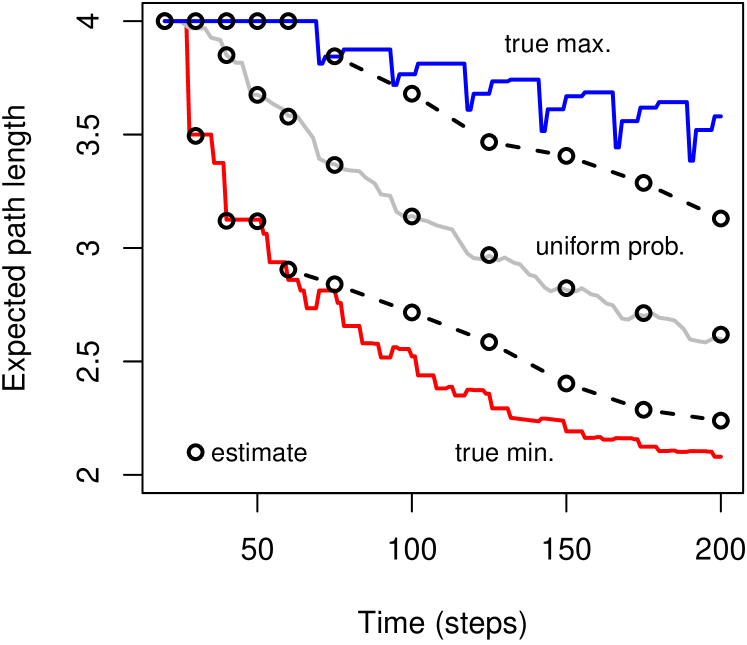
Figure 4: Gossip protocol.

The gossip protocol of [19] uses local connectivity to propagate information globally. Using a reachability reward property, our algorithms accurately estimate the expected minimum and maximum number of rounds necessary for the network to become connected as 1.486 and 4.5, compared to correct values 1.5 and 4.5. The average simulation time per estimate was approximately 1 minute.

Figure 4 plots the maximum and minimum estimated path length at different time steps, using an instantaneous reward property. The figure also plots the average estimates of the initial candidate set (generated in lines 2 to 2 of Algorithm 2). This average corresponds to the expected reward using the uniform probabilistic scheduler. The solid lines give the values calculated using numerical algorithms. The true value for the uniform probabilistic scheduler is calculated numerically by treating the MDP as a DTMC. We see that the estimates of maximum and minimum expected reward are accurate up to about 75 time steps, but less so above this value. The estimates are nevertheless guaranteed by (5) not to exceed the true values by more than a factor of $1+\varepsilon$ with probability $\delta$. Finally, we note that the average estimate of the initial candidate set is consistently accurate, demonstrating that Algorithm 1 is sampling correctly from scheduler space.

6.4 Choice Coordination

To demonstrate the scalability of our approach, we consider instances of the choice coordination model of [23] with $\mathit{BOUND}=100$. This value makes most of the models intractable to numerical model checking, however it is possible to infer the correct values of rewards from tractable instances. The chosen reachability property gives the expected minimum number of rounds necessary for a group of tourists to meet. The following table summarises the results:

Number of tourists	2	3	4	5	6	7	8	9	10
Minimum number of rounds to converge	4.0	5.0	7.0	8.0	10.0	11.0	12.0	13.0	14.0

All the estimates are exactly correct, while the average time to generate each result was just 8 seconds.

7 Prospects and Challenges

In this work we have focused on estimating the expected value of optimal rewards. We believe the same techniques may be immediately extended to sequential hypothesis testing, as in [22] and [9]. Ongoing work suggests that estimating rewards in continuous time models will also be feasible.

Overall, our case studies demonstrate that our approach is effective and can be efficient with state space that is intractable to numerical methods. While we do not yet provide confidence with respect to optimality, our techniques nevertheless generate useful conservative bounds with correct statistical guarantees of accuracy: the estimate will be greater (less) than the true maximum (minimum) expected reward by a factor of $\geq 1+\varepsilon$ with probability $\leq\delta$.

Figure 4 illustrates circumstances where the chosen per-iteration budget of $10^{5}$ is apparently not sufficient to explore the tails of the distribution of schedulers. Merely increasing the budget will not in general be adequate to address this problem, since near-optimal schedulers may be arbitrarily rare. Our proposed solutions are to (i) construct composite schedulers and (ii) sample from a property-specific subset of schedulers.

References

- [1] C. Baier and J.-P. Katoen. Principles of model checking. MIT Press, 2008.
- [2] R. Bellman. Dynamic Programming. Princeton University Press, 1957.
- [3] A. Bianco and L. De Alfaro. Model checking of probabilistic and nondeterministic systems. In Foundations of Software Technology and Theoretical Computer Science, pages 499–513. Springer, 1995.
- [4] J. Bogdoll, L. M. F. Fioriti, A. Hartmanns, and H. Hermanns. Partial order methods for statistical model checking and simulation. In Formal Techniques for Distributed Systems, pages 59–74. Springer, 2011.
- [5] B. Boyer, K. Corre, A. Legay, and S. Sedwards. PLASMA-lab: A flexible, distributable statistical model checking library. In K. Joshi, M. Siegle, M. Stoelinga, and P. D’Argenio, editors, Quantitative Evaluation of Systems, volume 8054 of LNCS, pages 160–164. Springer, 2013.
- [6] T. Brázdil, K. Chatterjee, M. Chmelík, V. Forejt, J. Křetínský, M. Kwiatkowska, D. Parker, and M. Ujma. Verification of markov decision processes using learning algorithms. In F. Cassez and J.-F. Raskin, editors, Automated Technology for Verification and Analysis, volume 8837 of Lecture Notes in Computer Science, pages 98–114. Springer, 2014.
- [7] H. S. Chang, J. Hu, M. C. Fu, and S. I. Marcus. Simulation-Based Algorithms for Markov Decision Processes. Springer, 2013.
- [8] T. H. Cormen, C. E. Leiserson, R. L. Rivest, and C. Stein. Introduction to Algorithms. MIT Press, edition, 2009.
- [9] P. D’Argenio, A. Legay, S. Sedwards, and L.-M. Traonouez. Smart sampling for lightweight verification of Markov decision processes. Submitted to International Journal on Software Tools for Technology Transfer, 2015.
- [10] A. Hartmanns and M. Timmer. On-the-fly confluence detection for statistical model checking. In NASA Formal Methods, pages 337–351. Springer, 2013.
- [11] D. Henriques, J. G. Martins, P. Zuliani, A. Platzer, and E. M. Clarke. Statistical model checking for Markov decision processes. In International Conference on Quantitative Evaluation of Systems (QEST2012), pages 84–93. IEEE, 2012.
- [12] W. Hoeffding. Probability inequalities for sums of bounded random variables. Journal of the American statistical association, 58(301):13–30, 1963.
- [13] W. G. Horner. A new method of solving numerical equations of all orders, by continuous approximation. Philosophical Transactions of the Royal Society of London, 109:308–335, 1819.
- [14] A. Israeli and M. Jalfon. Token management schemes and random walks yield self-stabilizating mutual exclusion. In Proc. Annual ACM Symposium on Principles of Distributed Computing (PODC ’90), pages 119–131. ACM New York, 1990.
- [15] C. Jegourel, A. Legay, and S. Sedwards. A platform for high performance statistical model checking – PLASMA. In Tools and Algorithms for the Construction and Analysis of Systems, volume 7214 of LNCS, pages 498–503. Springer, 2012.
- [16] M. Kearns, Y. Mansour, and A. Y. Ng. A sparse sampling algorithm for near-optimal planning in large Markov decision processes. Machine Learning, 49(2-3):193–208, 2002.
- [17] D. E. Knuth. The Art of Computer Programming. Addison-Wesley, edition, 1998.
- [18] M. Kwiatkowska, G. Norman, and D. Parker. Stochastic model checking. In M. Bernardo and J. Hillston, editors, Formal Methods for the Design of Computer, Communication and Software Systems: Performance Evaluation (SFM’07), volume 4486 of LNCS (Tutorial Volume), pages 220–270. Springer, 2007.
- [19] M. Kwiatkowska, G. Norman, and D. Parker. Analysis of a gossip protocol in PRISM. SIGMETRICS Perform. Eval. Rev., 36(3):17–22, Nov. 2008.
- [20] M. Kwiatkowska, G. Norman, D. Parker, and M. G. Vigliotti. Probabilistic mobile ambients. Theoretical Computer Science, 410(12-13):1272–1303, 2009.
- [21] R. Lassaigne and S. Peyronnet. Approximate planning and verification for large Markov decision processes. In Proc. Annual ACM Symposium on Applied Computing, pages 1314–1319. ACM, 2012.
- [22] A. Legay, S. Sedwards, and L.-M. Traonouez. Scalable verification of Markov decision processes. In Workshop on Formal Methods in the Development of Software (FMDS 2014), LNCS. Springer, 2014.
- [23] U. Ndukwu and A. McIver. An expectation transformer approach to predicate abstraction and data independence for probabilistic programs. In Proc. Workshop on Quantitative Aspects of Programming Languages (QAPL’10), 2010.
- [24] M. Okamoto. Some inequalities relating to the partial sum of binomial probabilities. Annals of the Institute of Statistical Mathematics, 10(1):29–35, 1958.
- [25] M. L. Puterman. Markov Decision Processes: Discrete Stochastic Dynamic Programming. Wiley-Interscience, 1994.
- [26] D. J. White. A survey of applications of Markov decision processes. Journal of the Operational Research Society, 44(11):1073–1096, Nov 1993.