Nonstationary filtered shot-noise processes and applications to neuronal membranes

Abstract

Filtered shot noise processes have proven to be very effective in modeling the evolution of systems exposed to shot noise sources and have been applied to a wide variety of fields ranging from electronics through biology. In particular, they can model the membrane potential $V_{m}$ of neurons driven by stochastic input, where these filtered processes are able to capture the nonstationary characteristics of $V_{m}$ fluctuations in response to presynaptic input with variable rate. In this paper we apply the general framework of Poisson point processes transformations to analyze these systems in the general case of nonstationary input rates. We obtain exact analytic expressions, as well as different approximations, for the joint cumulants of filtered shot noise processes with multiplicative noise. These general results are then applied to a model of neuronal membranes subject to conductance shot noise with a continuously variable rate of presynaptic spikes. We propose very effective approximations for the time evolution of the $V_{m}$ distribution and a simple method to estimate the presynaptic rate from a small number of $V_{m}$ traces. This work opens the perspective of obtaining analytic access to important statistical properties of conductance-based neuronal models such as the first passage time.

1 Introduction

We investigate the statistical properties of systems that can be described by the filtering of shot noise input through a linear first-order ordinary differential equation (ODE) with variable coefficients. Such systems give rise to filtered shot noise processes with multiplicative noise. The membrane potential $V_{m}$ fluctuations of neurons can be modeled as filtered shot noise currents or conductances (Verveen and DeFelice, 1974; Tuckwell, 1988). These fluctuations have been previously analyzed in the stationary limit of shot noise conductances with constant rate (Kuhn et al., 2004; Richardson and Gerstner, 2005; Rudolph and Destexhe, 2005; Burkitt, 2006a), and an exact analytical solution has been obtained for the mean and joint moments of exponential shot noise (Wolff and Lindner, 2008, 2010). However, many neuronal systems evolve in nonstationary regimes driven by shot noise with variable input rate. A typical example is provided by visual system neurons that receive presynaptic input with time-varying rate that reflects an evolving visual landscape. Modeling studies often consider the exponential shot noise case, whereas biological systems may display larger diversity including slow rising impulse response functions similar to alpha and bi-exponential functions, for example. Previous studies have addressed nonstationary exponential shot noise conductances and nonstationary currents (Cai et al., 2006; Amemori and Ishii, 2001; Burkitt, 2006b).

Poisson point processes (PPP) provide a natural model of random input arrival times that are distributed according to a Poisson law that may vary in time. Application-oriented treatments of PPP theory and PPP transformations can be found in Refs. (Moller and Waagepetersen, 2003; Streit, 2010). The key idea of this article is to express the filtered process as a transformation of random input arrival times and to apply the properties of PPP transformations to derive its nonstationary statistics. Using this formalism we derive exact analytical expressions for the mean and joint cumulants of the filtered process in the general case of variable input rate. We develop an approximation based on a power expansion of the expectation about the deterministic solution. We apply these results to a simple neuronal membrane model of sub-threshold membrane potential $V_{m}$ fluctuations that evolves under shot noise conductance with continuously variable rate of presynaptic spikes.

Shot noise processes are simple yet powerful models of stochastic input that correspond to the superposition of impulse responses arriving at random times according to a Poisson law. Systems evolving under shot noise input have been observed across many domains, such as electronics (Campbell, 1909; Schottky, 1918), optics (Picinbono et al., 1970; Rousseau, 1971), and many other fields (Snyder and Miller, 1991; Parzen, 1999). Shot noise was discovered in the early works of Campbell and Schottky (Campbell, 1909; Schottky, 1918). Key theoretical results were obtained by Rice (Rice, 1945) and a modern review of their probabilistic structure is presented in Ref. (Rice, 1977). Filtered shot noise processes with multiplicative noise are an extension of filtered Poisson process (Snyder and Miller, 1991; Parzen, 1999; Streit, 2010) that are generated by linear transformations of PPPs.

In this article, we start by presenting a simple model of filtered shot noise process with multiplicative noise and variable input rate (Sec. 2). We next consider the general case of PPP transformations and their properties (Sec. 3). Exact analytic expressions for the joint cumulants of the filtered process are derived (Sec. 4) in addition to an approximation of the exact analytical solution (Sec. 5). Finally, we apply these results to a simple neuronal membrane model of sub-threshold $V_{m}$ fluctuations with continuously variable rate of presynaptic spikes and explore several practical applications (Sec. 6).

2 Model of Filtered Shot Noise Process

In this section we present a simple model of filtered shot noise process with multiplicative noise. This stochastic process results from the filtering of shot noise input through a linear first-order ODE with variable coefficients. We show that under very simple input rate conditions the filtered process is nonstationary. We derive the time course of the filtered process in terms of the shot noise arrival times. The numerical simulation parameters are presented at the end of this section.

Consider the time evolution $Y(t)$ of a system governed by a linear first-order ODE with variable coefficients that is driven by shot noise input $Q(t)$:

$$\tau\frac{d}{dt}\,Y(t) =-Y(t)+\left(1-Y(t)\right)Q(t)$$ (1)

$$Q(t) =\sum_{x_{j}\in\xi}g(t-x_{j})\,H(t-x_{j})$$ (2)

where $\tau$ is a time constant, $\xi$ is the set of shot noise arrival times, $g(t-x_{j})\,H(t-x_{j})$ is the impulse response function at time $t$ for arrival time $x_{j}\in\xi$ and $H(u)$ is the Heaviside function. The impulse response function is also known as shot noise kernel.

The input arrival times $\xi$ in Eq. (2) are distributed according to a Poisson law as is characteristic of shot noise. The time evolution of this system is both stochastic and deterministic: stochastic since it is driven by random input arrival times $\xi$, but also deterministic since to each $\xi$ corresponds a unique outcome. The system response $Y(t,\xi)$ is said to be a filtered version of the shot noise process $Q(t,\xi)$ since Eq. (1) changes its spectral characteristics.

Nonstationary dynamics are introduced in the model by restricting input arrival times to occur between $t_{a}$ and $t_{b}\geq t_{a}$ with constant Poisson rate $\lambda$. A single realization of shot noise input $Q(t,\xi)$ and the resulting system response $Y(t,\xi)$ are shown in Fig. 1. The mean and standard deviation ($\mu\pm\sigma$) of both processes are clearly nonstationary since they vary in time.
The system response $Y(t,\xi)$ for a particular shot noise input $Q(t,\xi)$ is obtained by solving Eq. (1). For a given set of input arrival times $\xi$ and initial value $Y_{0}=0$,

$$Y(t,\xi) =\frac{1}{\tau}\int_{-\infty}^{t}e^{-\frac{t-z}{\tau}}\,Q(z,\xi)\,e^{-\frac{1}{\tau}\int_{z}^{t}Q(u,\xi)\,du}\,dz$$

$$=\frac{1}{\tau}\int_{-\infty}^{t}e^{-\frac{t-z}{\tau}}\,\sum_{x_{j}\in\xi}g(z-x_{j})\,H(z-x_{j})\prod_{x_{i}\in\xi}e^{-\frac{1}{\tau}\int_{z}^{t}g(u-x_{i})\,H(u-x_{i})\,du}\,dz$$ (3)

The input arrival times $\xi$ completely determine the time evolution of $Y(t,\xi)$. Equation (3) also shows that the response at time $t$ for each input arrival $x_{j}$ also depends on later input arrivals $x_{i}\leq t$. For a single shot noise source the solution can be further simplified using integration by parts:

$$Y(t,\xi) =1-\frac{1}{\tau}\int_{-\infty}^{t}e^{-\frac{t-z}{\tau}}\prod_{x_{i}\in\xi}e^{-\frac{1}{\tau}\int_{z}^{t}g(u-x_{i})\,H(u-x_{i})\,du}\,dz$$ (4)

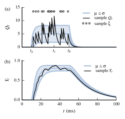
Figure 1: Single realization and basic statistics of filtered shot noise process $Y_{t}$ under shot noise input $Q_{t}$. (a) Random input arrival times $x_{j}\in\xi$ generate nonstationary shot noise $Q_{t}\equiv Q(t,\xi)$. The input arrival times are distributed with a variable Poisson rate $\lambda(t)$ that restricts the arrivals to occur between $t_{a}$ and $t_{b}$. (b) Nonstationary system response $Y_{t}\equiv Y(t,\xi)$ driven by shot noise $Q_{t}$. A single realization of random arrival times $\xi$ is represented by gray dots; realizations of $Q_{t}$ and $Y_{t}$ are shown in black lines. The mean and standard deviation ($\mu\pm\sigma$) of $Q_{t}$ and $Y_{t}$ are shown by gray lines and are clearly nonstationary.

The remainder of this article addresses the question of how to obtain the cumulants of the quantity on the left side of Eq. (4) from those on the right side, in the particular case of Poisson distributed input arrival times $\xi$ with variable rate $\lambda(t)$. For reasons of concise presentation, instead of Eq. (3), we consider the equivalent Eq. (4).

The numerical simulations were generated with the rate function $\lambda(t)$ represented in Fig. 2(a) and exponential kernel shot noise with $g(t-x)=h\exp\left(-(t-x)/\tau_{s}\right)$. Other parameters are $t_{max}=0.1$ s, $\tau=0.02$ s, $\lambda=500$ Hz, $h=4$ and $\tau_{s}=0.0025$ s.

3 Causal Point Process Transformations

We review the basic properties of PPP transformations and analyze the stochastic process generated by causal PPP transformations. The expectation of PPP transformations yields the joint cumulants of the associated processes. We illustrate this approach with the shot noise process and compare the predicted mean and second order cumulants with numerical simulations.

We consider a PPP $\Xi\,(\mathcal{S},\lambda)$ that generates points in the interval $\mathcal{S}\subseteq\mathbb{R}$ of the real line with rate function $\lambda(x)\geq 0$ such that $m(\mathcal{S})\equiv\int_{\mathcal{S}}\lambda(x)\,dx$ is finite for any bounded interval $\mathcal{S}$. A realization $\xi$ of $\Xi$ contains a set of $n\geq 0$ points $\{x_{1},\ldots,x_{n}\}\in\mathcal{S}$ that we associate with input arrival times. A PPP is said to be homogeneous for constant $\lambda(t)=\lambda$ and inhomogeneous otherwise. Example rate functions and sample realizations of the associated inhomogeneous PPP are shown in Fig. 2. These rate functions were used to generate input arrival times for the filtered shot noise process of Sec. 2 and the presynaptic spikes for the neuronal membrane of Sec. 6.

We consider a transformation $F(t,\xi)$ that for each real parameter $t\in\mathcal{S}$ and realization $\xi$ evaluates to a positive real number $F_{t}=F(t,\xi)$. The transformation is assumed invariant under permutation of $x_{j}\in\xi$, such that when written as a regular function we have $F(t,x_{1},\ldots,x_{n})=F(t,\{x_{1},\ldots,x_{n}\})$.
The expectation of $F(t,\xi)$ is obtained from the ensemble average over the number $n$ of points and their locations $\{x_{1},\ldots,x_{n}\}$:

$$\left\langle F(t,\xi)\right\rangle =\sum_{n=0}^{\infty}\frac{1}{n!}\,e^{-m(\mathcal{S})}\int_{\mathcal{S}}\cdots\int_{\mathcal{S}}F\left(t,x_{1},\ldots,x_{n}\right)\prod_{j=1}^{n}\lambda(x_{j})\,dx_{j}$$ (5)

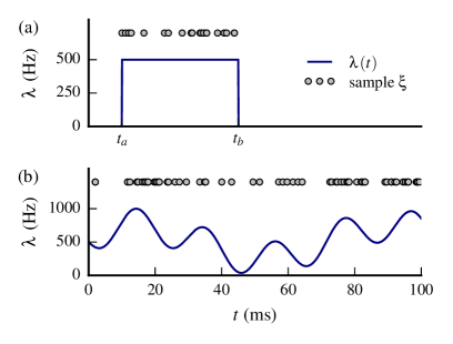
Figure 2: Rate function $\lambda(t)$ examples for inhomogeneous PPP. A single realization of input arrival times $\xi$ is represented by gray dots above the rate functions (blue lines) marking the location of input arrival times $x_{j}\in\xi$. (a) Rate function used to generate input arrival times for the filtered shot noise process of Sec. 2. (b) Rate function used to generate presynaptic spike times for the neuronal membrane of Sec. 6.

We now focus on the class of PPP transformations that are causal in the time parameter $t$. Such transformations ensure that arrivals $x_{j}\in\xi$ later than $t$ cannot affect the value of $F(t,\xi)$. A single realization $\xi$ generates the entire time course of $F(t,\xi)$ and we therefore associate a slave stochastic process $F_{t}\equiv F(t,\xi)$ to the causal PPP transformation $F(t,\xi)$. By construction, the expectation of $F_{t}$ is the expectation of $F(t,\xi)$ given by Eq. (5). This is illustrated in Fig. 3, where the value of shot noise process $F_{t}$ at different times is evaluated from the same realization $\xi$.

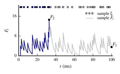
Figure 3: A shot noise process $F_{t}$ is a causal PPP transformation $F(t,\xi)$ of input arrival times $x_{j}\in\xi$. This particular PPP transformation is defined in Eq. (2) and its causality ensures that $F_{t}$ is not affected by input arrivals later than $t$. For example, the value of $F_{2}=F(t_{2},\xi)$ is determined by input arrivals $x_{j}\in\xi$ up to $t_{2}$ (blue line) and is not affected by input arrivals later than $t_{2}$ (light gray line). The dots above $F_{t}$ mark the location of input arrival times $x_{j}\in\xi$.

We write $F_{1},\ldots,F_{K}$ for the values of stochastic process $F_{t}$ at times $t_{1},\ldots,t_{K}$, $\left\langle F_{1}\cdots F_{K}\right\rangle$ for its joint moments and $\left\langle\left\langle F_{1}\cdots F_{K}\right\rangle\right\rangle$ for its joint cumulants. The expectation of PPP transformations enables to obtain analytical expressions for the joint moments and joint cumulants of $F_{t}$: its joint moments are obtained by evaluating the expectation of suitable products $F(t_{1},\xi)\cdots F(t_{K},\xi)$ and its joint cumulants can be constructed explicitly from the joint moments. For example, the moment $\left\langle F_{1}\,F_{2}^{2}\right\rangle$ is evaluated by the expectation $\left\langle F(t_{1},\xi)\,F(t_{2},\xi)^{2}\right\rangle$.

The causality of $F(t,\xi)$ enables to consider the PPP in the entire real line ($\mathcal{S}=\mathbb{R}$) with finite activity intervals constructed by setting $\lambda(t)=0$ outside the activity windows. This approach yields exact analytical expressions for the joint cumulants of nonstationary processes generated from causal PPP transformations as illustrated next with the nonstationary shot noise process from Sec. 2. A shot noise process is a particular type of random sum, which is a PPP transformation that factors as $F\left(t,\xi\right)=\sum_{x_{j}\in\xi}f(t,x_{j})$. The joint cumulants of random sums are given by the Campbell Theorem (Campbell, 1909; Rice, 1945) and are also derived for reference in Appendix A:

$$\left\langle\left\langle F_{1}\ldots F_{K}\right\rangle\right\rangle =\int_{\mathcal{S}}f(t_{1},x)\cdots f(t_{K},x)\,\lambda(x)\,dx$$ (6)

where $f(t,x)$ is the impulse response function at time $t$ for an input arrival time $x$. Shot noise is a causal random sum with $f(t,x)=g(t-x)\,H(t-x)$.

The expectation of more general forms of random sums, such as those in Eq. (3), are provided by the Slivnyak-Mecke Theorem (Slivnyak, 1962; Mecke, 1967). A comparison between numerical simulations and Campbell Theorem predictions is shown in Fig. 4 with excellent agreement for the mean and second order cumulants. The autocorrelation at times $t_{1}$ and $t_{2}$ is given by $\rho(F_{1}\,F_{2})=\left\langle\left\langle F_{1}\,F_{2}\right\rangle\right\rangle/(\sigma(F_{1})\,\sigma(F_{2}))$ where $\left\langle\left\langle F_{1}\,F_{2}\right\rangle\right\rangle$ is the autocovariance at times $t_{1}$ and $t_{2}$ and $\sigma(F_{t})$ is the standard deviation at time $t$.

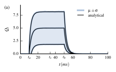
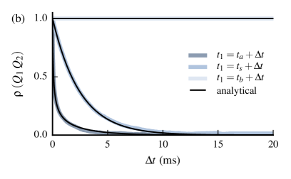
Figure 4: Comparison with numerical simulations for (a) the mean and standard deviation and (b) the autocorrelation of the shot noise process $Q_{t}$ from Sec. 2 as predicted by the Campbell Theorem (Eq. (6)). There is excellent agreement between the simulations (gray lines) and the analytic predictions (black lines) with the respective lines overlapping. The autocorrelation $\rho$ is evaluated at $t_{a}$, $t_{s}$, and $t_{b}$ corresponding respectively to the onset of PPP activity, quasi-stationary $Q_{t}$, and extinction of PPP activity.

4 Exact Analytical Solution

We use the properties of PPP transformations to derive exact analytical expressions for the cumulants of filtered shot noise processes with multiplicative noise and variable input rate. We investigate transformations that are relevant to these filtered processes: integral transform and random products. We evaluate their cumulants and compare with numerical simulations the predicted mean and second order cumulants of the filtered process.

According to Eq. (4), the filtered process $Y_{t}$ is the integral of a causal PPP transformation that factors as a product of exponentials of input arrival times $x_{j}\in\xi$. We now investigate these transformations and define an integral transform of $F(t,\xi)$ with regards to a positive and bounded function $w$:

$$SF(t,\xi) =\int_{-\infty}^{t}F(u,\xi)\,w(u,t)\,du$$ (7)

The mean and joint moments of the integral transform are calculated by interchanging the infinite sum and integrals of the expectation Eq. (5) with the integral of the transform provided any one side of the equalities is finite (Fubini-Tonelli Theorem).

$$\left\langle SF_{t}\right\rangle =\left\langle\int_{-\infty}^{t}F(u,\xi)\,w\left(u,t\right)du\right\rangle=\int_{-\infty}^{t}\left\langle F(u,\xi)\right\rangle w\left(u,t\right)du$$ (8)

$$\left\langle SF_{1}\cdots SF_{K}\right\rangle =\int_{-\infty}^{t_{1}}\cdots\int_{-\infty}^{t_{K}}\left\langle F(u_{1},\xi)\cdots F(u_{K},\xi)\right\rangle\prod_{l=1}^{K}w\left(u_{l},t_{l}\right)du_{l}$$ (9)

The linearity of integration extends Eq. (9) to the joint cumulants:

$$\left\langle\left\langle SF_{1}\cdots SF_{K}\right\rangle\right\rangle =\int_{-\infty}^{t_{1}}\cdots\int_{-\infty}^{t_{K}}\left\langle\left\langle F(u_{1},\xi)\cdots F(u_{K},\xi)\right\rangle\right\rangle\prod_{l=1}^{K}w\left(u_{l},t_{l}\right)du_{l}$$ (10)

We now analyze random products that are PPP transformations factoring as $F\left(t,\xi\right)=\prod_{x_{j}\in\xi}f(t,x_{j})$. The joint moments of random products are well known, and as shown in Appendix A:

$$\left\langle F_{1}\ldots F_{K}\right\rangle=\exp\left(\int_{\mathcal{S}}\left(\prod_{k=1}^{K}f(t_{k},x)-1\right)\lambda(x)\,dx\right)$$ (11)

We have gathered all the elements to derive the mean and joint cumulants of the filtered process $Y_{t}$. Writing $Q(t,\xi)=Q(t)$ and using the properties of joint cumulants,

$$\left\langle Y_{t}\right\rangle =1-\frac{1}{\tau}\int_{-\infty}^{t}\left\langle e^{-\frac{1}{\tau}\int_{z}^{t}Q(u)\,du}\right\rangle e^{-\frac{t-z}{\tau}}\,dz$$ (12)

$$\left\langle\left\langle Y_{1}\cdots\,Y_{K}\right\rangle\right\rangle =\left(-\frac{1}{\tau}\right)^{K}\int_{-\infty}^{t_{1}}\cdots\int_{-\infty}^{t_{K}}\left\langle\left\langle\prod_{k=1}^{K}e^{-\frac{1}{\tau}\int_{z_{k}}^{t_{k}}Q(u)\,du}\right\rangle\right\rangle\prod_{l=1}^{K}e^{-\frac{t_{l}-z_{l}}{\tau}}\,dz_{l}$$ (13)

The expectation of the random product of exponentials is obtained from Eq. (11) and yields:

$$\left\langle\prod_{k=1}^{K}e^{-\frac{1}{\tau}\int_{z_{k}}^{t_{k}}Q(u)\,du}\right\rangle =\exp\left(\int_{\mathcal{S}}\left(\prod_{k=1}^{K}e^{-\frac{1}{\tau}\int_{z_{k}}^{t_{k}}g(u-x)\,H(u-x)\,du}-1\right)\lambda(x)\,dx\right)$$ (14)

Replacing Eq. (14) into Eqs. (12) and (13) yields the exact solution for the joint cumulants of filtered shot noise process with multiplicative noise and variable input rate. The random product expectation of Eq. (14) is the key element in the evaluation of the mean and joint cumulants, which was already identified in previous work (Wolff and Lindner, 2008, 2010), where closed expressions were obtained for expo- nential kernel shot noise with constant rate. As our derivation shows, this extends to any shot noise kernel $g(t-x)\,H(t-x)$ and variable input rate $\lambda(t)$ and is the main original contribution of this work.

The comparison between numerical simulations and the predictions from Eqs. (12) and (13) are shown in Fig. 5. There is excellent agreement even in such a nonstationary scenario with the system undergoing transient evolution. The numerical evaluation of Eqs. (12) and (13) can be performed very efficiently with the trapezoidal rule due to the double exponential in the integrand.

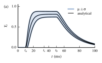
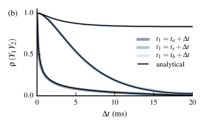
Figure 5: Comparison with numerical simulations for (a) the mean and standard deviation and (b) the autocorrelation of the filtered process $Y_{t}$ predicted by the exact analytic solution given by Eqs. (12) and (13). There is excellent agreement between the simulations (gray lines) and the analytic predictions (black lines) with the respective lines overlapping. The autocorrelation $\rho$ is evaluated at $t_{a}$, $t_{s}$, and $t_{b}$ corresponding respectively to the onset of PPP activity, quasi-stationary $Y_{t}$, and extinction of PPP activity.

5 Central Moments Expansion

We propose an approximation of the exact analytical solution that is based on a power expansion about the deterministic solution. The central moments expansion (CME) yields a series in the central moments of integrated shot noise. We compare this approximation for the mean and second order cumulants with numerical simulations, including the case of constant Poison rate.

The deterministic solution of Eq. (1) with mean shot noise input $\left\langle Q(u)\right\rangle$ is given by:

$$\left\langle Y_{t}\right\rangle_{0} =1-\frac{1}{\tau}\int_{-\infty}^{t}e^{-\frac{t-z}{\tau}}e^{-\frac{1}{\tau}\int_{z}^{t}\left\langle Q(u)\right\rangle\,du}\,dz$$

This suggests an expansion about the deterministic solution $\left\langle Y_{t}\right\rangle_{0}$ by performing power expansions of the random product expectations in Eqs. (12) and (13). The integrated mean shot noise is first factored out of the random product and a power expansion of the resulting exponential is performed. This corresponds to the delta method technique (Cramér, 1946; Oehlert, 1992) for approximating expectations of random variable transformations and yields a series in the central moments of integrated shot noise. As shown in Appendix B, the second order expansion for a single random product yields:

$$\left\langle e^{-\frac{1}{\tau}\int_{z}^{t}Q(u)\,du}\right\rangle \simeq e^{-\frac{1}{\tau}\int_{z}^{t}\left\langle Q(u)\right\rangle du}\left(1+\frac{1}{2}\left\langle\left(-\frac{1}{\tau}\int_{z}^{t}\left(Q(u)-\left\langle Q(u)\right\rangle\right)du\right)^{2}\right\rangle\right)$$

This provides the following approximation for the mean of the filtered process:

$$\left\langle Y_{t}\right\rangle_{2} =1-\frac{1}{\tau}\int_{-\infty}^{t}e^{-\frac{1}{\tau}\int_{z}^{t}\left(1+\left\langle Q(u)\right\rangle\right)du}\left(1+\frac{1}{2\tau^{2}}\int_{z}^{t}\int_{z}^{t}\left\langle\left\langle Q(u_{1})\,Q(u_{2})\right\rangle\right\rangle du_{1}\,du_{2}\right)dz$$ (15)

where the subscript 2 represents the second order of the expansion.

Extending to joint cumulants is straightforward by expanding each exponential individually and collecting terms of same order in $1/\tau$. The first order expansion for the autocovariance is given by:

$$\left\langle\left\langle Y_{1}\,Y_{2}\right\rangle\right\rangle_{1} =\frac{1}{\tau^{4}}\int_{-\infty}^{t_{1}}\int_{-\infty}^{t_{2}}e^{-\frac{1}{\tau}\int_{z_{1}}^{t_{1}}\left(1+\left\langle Q(u)\right\rangle\right)du-\frac{1}{\tau}\int_{z_{2}}^{t_{2}}\left(1+\left\langle Q(v)\right\rangle\right)dv}\int_{z_{1}}^{t_{1}}\int_{z_{2}}^{t_{2}}\left\langle\left\langle Q(u_{1})\,Q(u_{2})\right\rangle\right\rangle du_{1}\,du_{2}\,dz_{1}\,dz_{2}$$ (16)

The first order expansion for the variance is obtained from Eq. (16) by replacing $t_{1}=t_{2}=t$. The comparison between numerical simulations and the predictions from Eqs. (15) and (16) are shown in Fig. 6. There is good agreement for the mean but lower accuracy for second order cumulants. This can be improved with the second order expansion for the autocovariance that is provided in Appendix B.

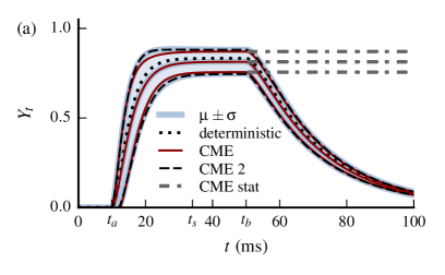
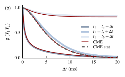
Figure 6: Comparison with numerical simulations for (a) the mean and standard deviation and (b) the autocorrelation of the central moments expansion given by Eqs. (15) and (16). There is good agreement between the simulations (full gray lines) and the approximation (full red lines) for the mean but lower accuracy for second order cumulants. This is corrected by the second order expansion for the autocovariance (dashed black lines) that is provided in Appendix B. The stationary limit (dashed dotted gray lines) is also shown. The deterministic solution (dotted black line) displays considerable approximation error.

We found that the second order expansion for the mean and autocovariance consistently provided good results in the parameter regimes of neuron cells (as seen in Fig. 6(a) and Fig. 9 below). Under these conditions, third and fourth order expansions either did not provide significant improvements over the second order or even resulted in worse approximations, in which case much higher order expansions would be required to improve on the second order. Under certain parameter regimes the first order expansion for the autocovariance (Eq. (16)) may already provide good results (see Fig. 8 below).

The stationary limit of the filtered process reflects the statistics of long running trials under shot noise input with constant rate. The cumulants for this regime can be obtained by placing the onset of input arrival times at $-\infty$ and replacing the mean and second order cumulants of shot noise in Eqs (15) and (16) with their stationary limits. After integration by parts,

$$\left\langle Y_{t}\right\rangle_{2} =\frac{\left\langle Q\right\rangle}{1+\left\langle Q\right\rangle}-\frac{\left\langle\left\langle Q^{2}\right\rangle\right\rangle}{\left(1+\left\langle Q\right\rangle\right)^{2}}\frac{1}{\tau}\int_{-\infty}^{t}e^{-\frac{t-z}{\tau}\left(1+\left\langle Q\right\rangle\right)}\,r\left(t-z\right)dz$$ (17)

$$\left\langle\left\langle Y_{1}\,Y_{2}\right\rangle\right\rangle_{1} =\frac{\left\langle\left\langle Q^{2}\right\rangle\right\rangle}{\left(1+\left\langle Q\right\rangle\right)^{2}}\frac{1}{\tau^{2}}\int_{-\infty}^{t_{1}}\int_{-\infty}^{t_{2}}e^{-\frac{t_{1}-z_{1}+t_{2}-z_{2}}{\tau}\left(1+\left\langle Q\right\rangle\right)}\,r\left(|z_{1}-z_{2}|\right)dz_{1}\,dz_{2}$$ (18)

where $\left\langle Q\right\rangle$, $\left\langle\left\langle Q^{2}\right\rangle\right\rangle$ and $\left\langle\left\langle Q_{1}\,Q_{2}\right\rangle\right\rangle=\left\langle\left\langle Q^{2}\right\rangle\right\rangle r\left(|t_{1}-t_{2}|\right)$ are, respectively, the mean, variance, and autocovariance of stationary shot noise.

The stationary limits for the mean and second order cumulants of the exponential and alpha kernels are presented in Appendix B.1.

6 Application to Neuronal Membranes

We apply the previous results to a simple model of membrane potential $V_{m}(t)$ fluctuations and explore several practical applications. We first calculate the nonstationary cumulants and compare them with numerical simulations. The central moment expansion (CME) is compared with previously published analytical estimates for the stationary limit of $V_{m}(t)$. The nonstationary cumulants are integrated in truncated Edgeworth series to approximate the time-evolving distribution of $V_{m}(t)$, which is compared with numerical simulations. We propose a simple method to estimate $\lambda(t)$ from a small number of noisy realizations of $V_{m}(t)$ and compare the inferred rate to the original presynaptic rate function. The numerical simulation parameters are presented below.

We consider a simple model of the membrane potential $V_{m}(t)$ for a passive neuron without spiking mechanism that is driven by shot noise conductance $G(t)$. This model has a single synapse type and is directly applicable to experiments where one type of synapse is isolated (Okun and Lampl, 2008). The time evolution of $V_{m}(t)$ under conductance shot noise input $G(t)$ is given by the following membrane equation:

$$\tau_{m}\,\frac{d}{dt}\,V_{m}(t) =E_{l}-V_{m}(t)+\left(E_{s}-V_{m}(t)\right)\frac{1}{g_{l}}\,G(t)$$ (19)

$$\frac{1}{g_{l}}\,G(t) =\sum_{x_{j}\in\xi}g(t-x_{j})\,H(t-x_{j})$$ (20)

where $\tau_{m}$ is the membrane time constant, $E_{l}$ is the resting potential, $E_{s}$ is the synaptic reversal potential, $g_{l}$ is the leak conductance and $\xi$ is a set of presynaptic spike times.

The membrane equation is a scaled and translated version of Eq. (1) with the following change of variables:

$$V_{m}(t)=\left(E_{s}-E_{l}\right)Y(t)+E_{l} Q(t)=\frac{1}{g_{l}}\,G(t)$$

A single realization of conductance shot noise $G_{t}\equiv G(t,\xi)$ and the resulting membrane potential response $V_{t}\equiv V_{m}(t,\xi)$ are shown in Fig. 7, where the mean and standard deviation of both processes are also represented. The numerical simulations were generated with the rate function $\lambda(t)$ represented in Fig. 2(b) and alpha kernel shot noise with $g(t-x)=h(t-x/\tau_{s})\exp\left(-(t-x)/\tau_{s}\right)$. Other parameters are $\tau_{m}=0.02$ s, $E_{l}=-0.06$ V, $E_{s}=0$ V and $g_{l}=10\text{\sc{e}-}9$ S in addition to those detailed in Section 2. The quantal conductance is $4\text{\sc{e}-}9$ S corresponding to $h=0.4$.

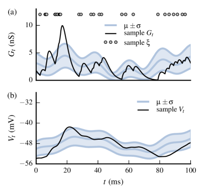
Figure 7: Single realization and basic statistics of membrane potential $V_{t}$ fluctuations under conductance shot noise input $G_{t}$. (a) Random presynaptic spike times $x_{j}\in\xi$ generate nonstationary shot noise conductance $G_{t}\equiv G(t,\xi)$. The presynaptic spike times are distributed with a continuously varying rate $\lambda(t)$. (b) Nonstationary membrane potential $V_{t}\equiv V(t,\xi)$ driven by shot noise conductance $G_{t}$. A single realization of spike times $\xi$ is represented by gray dots; realizations of $G_{t}$ and $V_{t}$ are shown in black lines. The mean and standard deviation ($\mu\pm\sigma$) of $G_{t}$ and $V_{t}$ are shown with gray lines.

6.1 Nonstationary Cumulants

A first application of this formalism is to derive the mean and joint cumulants of $V_{t}$ from those of $Y_{t}$. Using the properties of the mean and cumulants of random variables for each value of $t$ yields the required relationships:

$$\left\langle V_{t}\right\rangle =(E_{s}-E_{l})\left\langle Y_{t}\right\rangle+E_{l} \left\langle\left\langle V_{1}\cdots V_{K}\right\rangle\right\rangle=(E_{s}-E_{l})^{K}\left\langle\left\langle Y_{1}\cdots Y_{K}\right\rangle\right\rangle$$ (21)

The comparison between numerical simulations and the predictions from Eq. (21) is shown in Fig. 8. There is excellent agreement with the predictions from both the exact analytical solution given by Eqs. (12) and (13) and the CME given by Eqs (15) and (16). The deterministic solution is obtained from Eq. (21) by replacing $\left\langle Y_{t}\right\rangle$ with $\left\langle Y_{t}\right\rangle_{0}$ and displays good agreement with mean $V_{t}$.

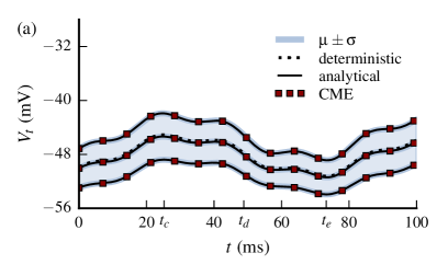
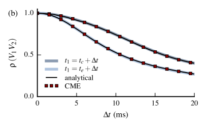
Figure 8: Comparison with numerical simulations for (a) the mean and standard deviation and (b) the autocorrelation of membrane potential $V_{t}$ predicted by the exact analytical solution (full black lines) and the central moments expansion (red squares). There is excellent agreement between the simulations (full gray lines) and the analytic prediction for both methods with the respective lines overlapping. The deterministic solution (dotted black line) also displays good agreement with mean $V_{t}$. The autocorrelation $\rho$ is evaluated at local maxima ($t_{c}$) and minima ($t_{e}$) of mean $V_{t}$.

In this parameter regime, the approximation error of the CME is very low (on the order of $0.01$ mV). However, additional terms of the expansion may be required to reach similar precision in other parameter regimes. In order to illustrate this, we increase the quantal conductance by a factor of 20 (to 80 nS) with the effect of raising mean $V_{t}$ very close to the reversal potential $E_{s}$. As shown in Fig. 9, the CME is still in very good agreement for the mean but the approximation error is larger for the standard deviation (on the order of several millivolts). The second order expansion for the standard deviation results in lower approximation error (in the order of 1 mV) but requires evaluating third and fourth order cumulants of integrated shot noise. The approximation error for the deterministic solution also increases to several mV.

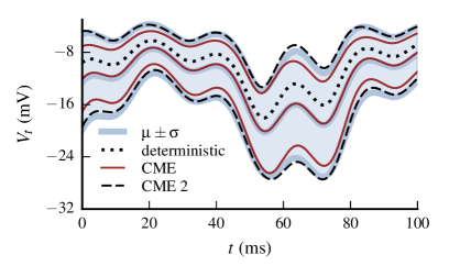
Figure 9: Same parameter regime as Fig. 8 but with quantal conductance increased by a factor of 20 ($h=80$ nS). The mean and standard deviation of the numerical simulations (full gray lines) display excellent agreement with the exact analytical solution but are omitted for clarity. The approximation error for the CME (full red lines) remains low for the mean but increases significantly for both the standard deviation and the deterministic solution (dotted black line). The second order expansion for the standard deviation (dashed black lines) results in lower approximation error.

The Appendix B.2 provides analytical expressions for the CME in the stationary limit of $V_{t}$ for the mean and second order cumulants of exponential and alpha kernels. These expressions are obtained by applying Eq. (21) to Eqs. (17) and (18) and are consistent with previous analytical estimates for the mean and standard deviation that were derived with different approaches: Fokker-Planck methods for exponential kernel shot noise (Richardson and Gerstner, 2005; Rudolph and Destexhe, 2005) given by Eqs. (24), and a shot noise approach for alpha kernel shot noise (Kuhn et al., 2004) given by Eqs. (29). The extension to the autocovariance is given by Eqs. (28), and (35) respectively.

6.2 Probability Distribution Approximation

A second application of this formalism is to use the nonstationary cumulants to approximate the time evolving distribution of membrane potential fluctuations. The mean and standard deviation of $V_{t}$ yield a Gaussian approximation that successfully captures the time evolution of $p(V_{t})$ as illustrated in Fig. 10. As expected, the skew of the distribution is not well captured by the Gaussian approximation, which has been reported in both experimental (Destexhe and Paré, 1999) and theoretical studies (Richardson and Gerstner, 2005; Rudolph and Destexhe, 2005). The quantal conductance was increased by a factor of 4 (to 16 nS) in these simulations.

Deviations from the Gaussian distribution are expected whenever cumulants of order three or higher are present in $p(V_{t})$. We use a truncated Edgeworth series (Edgeworth, 1907; Cramér, 1946; Wallace, 1958) to account for these deviations since it provides an asymptotic expansion of $p(V_{t})$ in terms of its cumulants. In particular, we use the Edgeworth series expanded from the Gaussian distribution distribution as discussed in (Badel, 2011). This has the advantage of coinciding with the Gaussian approximation whenever cumulants of order three or higher are negligible. This is an important aspect since approximately Gaussian shapes of $p(V_{t})$ are sometimes present in experimental intracellular recordings. In terms of the normalized process $X_{t}=\left(V_{t}-\left\langle V_{t}\right\rangle\right)/\sigma_{t}$ with $\sigma_{t}\equiv\sqrt{\left\langle\left\langle V_{t}^{2}\right\rangle\right\rangle}$, the truncated fourth order Edgeworth series is given by:

$$p_{Ew4}\left(X_{t}=x\right) =\frac{1}{\sigma_{t}}\left(1+\frac{1}{3!}\frac{\left\langle\left\langle V_{t}^{3}\right\rangle\right\rangle}{\sigma_{t}^{3}}\left(x^{3}-3x\right)\right.$$

$$\qquad\qquad\left.+\frac{1}{4!}\frac{\left\langle\left\langle V_{t}^{4}\right\rangle\right\rangle}{\sigma_{t}^{4}}\left(x^{4}-6x^{2}+3\right)+\frac{10}{6!}\frac{\left\langle\left\langle V_{t}^{3}\right\rangle\right\rangle^{2}}{\sigma_{t}^{6}}\left(x^{6}-15x^{4}+45x^{2}-15\right)\right)\mathcal{N}(x)$$ (22)

where $\mathcal{N}(x)=\exp(-x^{2}/2)/\sqrt{2\pi}$ is the standard normal density and $p(V_{t}=v)\simeq p_{Ew}\left(x=\frac{v-\left\langle V_{t}\right\rangle}{\sigma_{t}}\right)$. The third order Edgeworth series is given by the the first two terms.

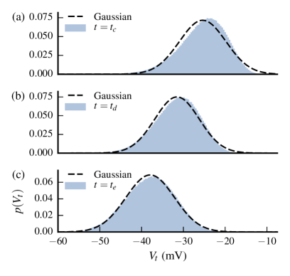
Figure 10: Nonstationary density of membrane potential $p(V_{t})$ evaluated at three different times times: $t_{c}$, $t_{d}$, and $t_{e}$ corresponding to (a), (b), and (c), respectively, (see abscissa of Fig. 8(a)). Comparison between the empirical histogram (gray) and the Gaussian approximation (dashed line) based on nonstationary mean and variance of $V_{t}$. The time evolution of $p(V_{t})$ is captured successfully by this approximation, which as expected also misses the skew of $p(V_{t})$.

As illustrated in the left side of Fig. 11, the skewness of $p(V_{t})$ is indeed captured by the third order of the Edgeworth series. Figure 11(c) also shows a slight overestimation near the peak of $p(V_{t})$, which is successfully captured by the fourth order, as shown in the right side of this figure.

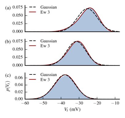
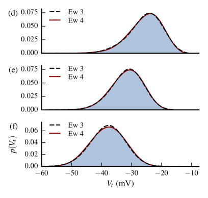
Figure 11: (a)-(c): Comparison at times $t_{c}$, $t_{d}$, and $t_{e}$ between the empirical histogram (gray), Gaussian approximation (dashed black line), and the third order Edgeworth series (full red line). (d)-(f): Comparison at times $t_{c}$, $t_{d}$, and $t_{e}$ between the empirical histogram (gray), third order Edgeworth series (dashed black line), and fourth order Edgeworth series (full red line). The slight discrepancy at the peak of the empirical histogram in (c) is successfully captured by the fourth order Edgeworth series in (f).

Under more extreme parameter regimes, additional terms of the Edgeworth series may be needed to approximate $p(V_{t})$. In such cases, the asymptotic character of the series becomes relevant since the truncation error is of the same order as the first neglected term of the series. An important caveat is that the truncated series may yield negative values for certain values of $x$. This is intrinsic to Edgeworth series that are constructed in the set of orthogonal polynomials associated with the base distribution (Hermite polynomials in the case of the standard normal distribution). The truncated series integrates to unity but may result in an invalid density function since negatives values are possible. Algorithms for computing an Edgeworth series to an arbitrary order are provided in Refs. (Petrov, 1962; Blinnikov and Moessner, 1998).

6.3 presynaptic Rate Estimation

Another application of this formalism is to estimate the nonstationary presynaptic rate $\lambda(t)$ from a small number ($N=10$) of membrane potential $V_{t}$ traces that are independently generated from the same PPP. Each trace has small amounts of additive noise to simulate measurement error that are independent from the PPP. The traces of $V_{t}$ are sampled at rate $1/\Delta t$. A single realization of the noisy membrane potential with mean and variance estimated from a small number of traces is shown in Fig. 12. The noisy membrane equation is given by:

$$\tau_{m}\,\frac{d}{dt}\,V_{m}(t) =E_{l}-V_{m}(t)+\left(E_{s}-V_{m}(t)\right)\frac{1}{g_{l}}\,G(t)+\epsilon(t)$$ (23)

where $\epsilon(t)$ is a zero mean Gaussian white noise in units of voltage with $\sigma(\epsilon)=0.2$ mV.

The key expression that enables to estimate $\lambda(t)$ from traces of $V_{t}$ is the Campbell Theorem for the mean of nonstationary shot noise given by Eq. (6). If the shot noise kernel is known then the rate function can in principle be obtained by deconvolution of the mean conductance. However, this operation is very sensitive to noise since small changes in the estimated mean conductance will result in large changes of the estimated rate function. This aspect is dealt with by smoothing the estimated mean conductance prior to performing the deconvolution step. From each trace of $V_{t}$ we extract the input conductance by inverting Eq. (23) and average them to obtain the estimated mean conductance:

$$\left\langle\hat{G}_{t}\right\rangle =\frac{1}{N}\sum_{n=1}^{N}\frac{g_{l}}{\Delta t}\,\frac{\tau_{m}\left(V_{t+\Delta t}^{n}-V_{t}^{n}\right)-\Delta t\left(E_{l}-V_{t}^{n}\right)}{E_{s}-V_{t}^{n}}$$

where $V_{t}^{n}$ is the $n$-th trace of $V_{t}$ and $\Delta t$ is the sampling interval.

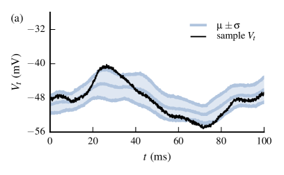
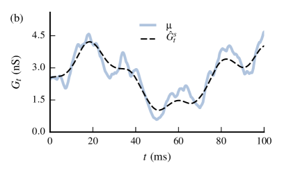
Figure 12: (a) Single realization (black line) and basic statistics (gray lines) generated from a small number ($N=10$) of membrane potential $V_{t}$ traces with additive noise to simulate measurement error. (b) Extracted mean conductance (full gray line) and smoothed version $G_{t}^{s}$ (dashed black line) obtained with non-parametric smoothing.

The estimated mean conductance will be a noisy version of the actual mean conductance due to the effects of the additive noise $\epsilon(t)$ in each trace of $V_{t}$. Non-parametric smoothing is performed using a local linear smoother with tricube kernel and kernel bandwidth selected by cross-validation (Wasserman, 2006), yielding the smoothed version $\left\langle\hat{G}_{t}^{s}\right\rangle$ shown in Fig. 12(b). Finally, we use the discrete convolution theorem to estimate the presynaptic rate $\hat{\lambda}(t)$ from the smoothed mean conductance:

$$\hat{\lambda}(t) =\frac{1}{\Delta t}\,\text{DFT}^{-1}\left[\frac{\text{DFT}\left\{\left\langle\hat{G}_{t}^{s}\right\rangle\right\}}{\text{DFT}\{g\}}\right]$$

The result is shown in Fig. 13, where the estimated $\hat{\lambda}(t)$ rate compares favorably to the original presynaptic rate $\lambda(t)$. Estimating $\lambda(t)$ from noisy shot noise data has been previously addressed (Sequeira and Gubner, 1995) in addition to methods that enable to estimate the shot noise kernel (Sequeira and Gubner, 1997).

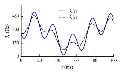
Figure 13: Estimated presynaptic rate $\hat{\lambda}(t)$ (black dashed line) compared with original rate function $\lambda(t)$ (full blue line). The magnitude and variations are reasonably well captured considering the small number ($N=10$) of membrane potential traces used.

7 Discussion

In this paper, we investigated important statistical properties of filtered shot noise processes with multiplicative noise, in the general case of variable input rate. These properties provide a compact description of time-evolving dynamics of the system. Such processes arise from the filtering of nonstationary shot noise input through a linear first-order ODE with variable coefficients. We have obtained general results for this class of stochastic processes and results specific to applications in neuronal models.

We first identified the causal PPP transformation that corresponds to filtered shot noise with multiplicative noise. We investigated the statistical properties of this transformation to derive the exact analytical solution for the joint cumulants of the filtered process with variable input rate. Excellent agreement with numerical simulations was found for the mean and second order cumulants. We proposed an approximation based on a CME about the solution of the deterministic system. We have shown with numerical simulations that under parameter regimes relevant to neuronal membranes the second order of this approximation provides good results for the mean and second order cumulants. Under certain parameter regimes, the first order expansion for the second order cumulants may already provide effective approximations.

These general results were then applied to a simple model of subthreshold membrane potential $V_{m}$ fluctuations subject to shot noise conductance with continuously variable rate of presynaptic spikes. Excellent agreement with numerical simulations was found for the mean and second order cumulants for both the exact analytical solution and the second order CME. This approximation is consistent with previously published analytical estimates for stationary $V_{m}$ . An expression for the stationary limit of autocovariance is provided for exponential and alpha kernel shot noise input. An approximation for the time-evolving distribution of $V_{m}$ is proposed that is based on a truncated Edegeworth series using the nonstationary cumulants obtained analytically. This approximation successfully captures the time evolution of $V_{m}$ under a large range of conditions. The nonstationary mean of shot noise is used to estimate the presynaptic rate from a small number of intracellular $V_{m}$ recordings with additive noise simulating measurement error.

In future work we will extend this formalism to multiple independent shot noise inputs by applying the Slivnyak-Mecke Theorem. Such development would yield direct applications for neuronal membrane models with different synapse types (such as excitatory and inhibitory synapses). Preliminary work indicates that analytic treatment of filtered shot noise with correlated input is accessible with this formalism. The present work also opens perspectives for the analytical development first passage time statistics based on nonstationary approxima- tions of the filtered process distribution.

Acknowledgments

Research was supported by the CNRS, the Agence Nationale de la Recherche (ANR; ComplexV1 project), and the European Community (BrainScales FP7-269921 and the Human Brain Project FP7-604102). M.B. was supported by a PhD fellowship from the European Marie-Curie Program (FACETS-ITN FP7-237955).

Appendix

Appendix A Random Sums and Random Products

Random products are transformations of PPP that factor as $F\left(t,\xi\right)=\prod_{x_{j}\in\xi}f(t,x_{j})$. The expectation of random products is obtained as follows:

$$\left\langle F_{t}\right\rangle =\sum_{n=0}^{\infty}\frac{1}{n!}\,e^{-m(\mathcal{S})}\left(\int_{\mathcal{S}}f(t,x)\,\lambda(x)\,dx\right)^{n}=\exp\left(\int_{\mathcal{S}}\left(f(t,x)-1\right)\lambda(x)\,dx\right)$$

$$\left\langle F_{1}\ldots F_{K}\right\rangle =\left\langle\prod\limits_{x_{j}\in\xi}\prod\limits_{k=1}^{K}f(t_{k},x_{j})\right\rangle=\exp\left(\int_{\mathcal{S}}\left(f(t_{1},x)\cdots f(t_{K},x)-1\right)\lambda(x)\,dx\right)$$

In the case of the random product with $f(t,x_{j})=e^{-\frac{1}{\tau}\int_{z}^{t}g(u-x_{j})H(u-x_{j})du}$ and $\mathcal{S}=\mathbb{R}$,

$$\left\langle e^{-\frac{1}{\tau}\int_{z}^{t}Q(u,\xi)\,du}\right\rangle =\exp\left(\int_{-\infty}^{z}\left(e^{-\frac{1}{\tau}\int_{z}^{t}g(u-x)\,du}-1\right)\lambda(x)\,dx+\int_{z}^{t}\left(e^{-\frac{1}{\tau}\int_{y}^{t}g(v-y)\,dv}-1\right)\lambda(y)\,dy\right)$$

Random sums are transformations of PPP that factor as $F\left(t,\xi\right)=\sum_{x_{j}\in\xi}f(t,x_{j})$. The joint cumulants of random sums are given by the Campbell Theorem (Campbell, 1909; Rice, 1945). The characteristic function $\phi(s_{1},\ldots,s_{K})$ is the expectation of a random product, and its derivatives yield the joint cumulants:

$$\phi(s_{1},\ldots,s_{K}) \equiv\left\langle e^{is_{1}F(t_{1},\xi)+\cdots+is_{K}F(t_{K},\xi)}\right\rangle=\left\langle\prod_{x_{j}\in\xi}\prod_{k=1}^{K}e^{is_{k}f(t_{k},x_{j})}\right\rangle=\exp\left(\int_{\mathcal{S}}\left(e^{\sum_{k=1}^{K}is_{k}f(t_{k},x)}-1\right)\lambda(x)\,dx\right)$$

$$\left\langle\left\langle F(t_{1},\xi)\ldots F(t_{K},\xi)\right\rangle\right\rangle =\left.\left(\frac{1}{i}\,\frac{d}{ds_{1}}\right)\cdots\left(\frac{1}{i}\,\frac{d}{ds_{K}}\right)\ln\phi(s_{1},\ldots,s_{K})\right|_{s_{1},\ldots,s_{K}=0}=\int_{\mathcal{S}}f(t_{1},x)\cdots f(t_{K},x)\,\lambda(x)\,dx$$

Appendix B Central Moments Expansion

A Taylor expansion of the random product about mean shot noise input results in a series of central moments of the integrated shot noise. Expanding the exponential inside the expectation, keeping terms of order $(1/\tau_{m})^{2}$ and re-expressing in terms of cumulants, yields:

$$\left\langle e^{-\frac{1}{\tau}\int_{z}^{t}Q(u,\xi)\,du}\right\rangle =e^{-\frac{1}{\tau}\int_{z}^{t}\left\langle Q(u)\right\rangle du}\left(1+\sum_{m=2}^{+\infty}\frac{1}{m!}\left\langle\left(-\frac{1}{\tau}\int_{z}^{t}\left(Q(u,\xi)-\left\langle Q(u)\right\rangle\right)\,du\right)^{m}\right\rangle\right)$$

$$\simeq e^{-\frac{1}{\tau}S\bar{Q}}\left(1+\frac{1}{2\,\tau^{2}}\left\langle\left\langle SQ^{2}\right\rangle\right\rangle\right)$$

where $SQ^{2}\equiv\int_{z}^{t}Q^{2}(v,\xi)\,dv$ and $S\bar{Q}\equiv\int_{z}^{t}\left\langle Q(u)\right\rangle\,du$.

Higher order cumulants are obtained in a similar manner by expanding each exponential individually and collecting terms in the same order of $1/\tau_{m}$. The second order expansion for second order cumulants involves the expansion of two random products and keeping terms up to order $(1/\tau_{m})^{4}$, yielding:

$$\left\langle\left\langle e^{-\frac{1}{\tau}\int_{z_{1}}^{t_{1}}Q(u_{1},\xi)\,du_{1}}\,e^{-\frac{1}{\tau}\int_{z_{2}}^{t_{2}}Q(u_{2},\xi)\,du_{2}}\right\rangle\right\rangle$$

$$\quad\simeq e^{-\frac{1}{\tau}S\bar{Q}_{1}-\frac{1}{\tau}S\bar{Q}_{2}}\Bigg{(}\frac{1}{\tau^{2}}\left\langle\left\langle SQ_{1}\,SQ_{2}\right\rangle\right\rangle-\frac{1}{2\tau^{3}}\left(\left\langle\left\langle SQ_{1}^{2}\,SQ_{2}\right\rangle\right\rangle+\left\langle\left\langle SQ_{1}\,SQ_{2}^{2}\right\rangle\right\rangle\right)$$

$$\qquad\qquad\qquad\qquad\quad+\frac{1}{2\tau^{4}}\Big{(}\frac{1}{3}\left\langle\left\langle SQ_{1}^{3}\,SQ_{2}\right\rangle\right\rangle+\frac{1}{3}\left\langle\left\langle SQ_{1}\,SQ_{2}^{3}\right\rangle\right\rangle+\frac{1}{2}\left\langle\left\langle SQ_{1}^{2}\,SQ_{2}^{2}\right\rangle\right\rangle$$

$$\qquad\qquad\qquad\qquad\qquad\qquad+\left\langle\left\langle SQ_{1}\,SQ_{2}\right\rangle\right\rangle\left(\left\langle\left\langle SQ_{1}^{2}\right\rangle\right\rangle+\left\langle\left\langle SQ_{2}^{2}\right\rangle\right\rangle+\left\langle\left\langle SQ_{1}\,SQ_{2}\right\rangle\right\rangle\right)\Big{)}\Bigg{)}$$

where $SQ_{1}\equiv\int_{z_{1}}^{t_{1}}Q(v,\xi)\,dv$, $SQ_{1}^{2}\equiv\int_{z_{1}}^{t_{1}}Q^{2}(v,\xi)\,dv$ and $S\bar{Q}_{1}\equiv\int_{z_{1}}^{t_{1}}\left\langle Q(u)\right\rangle\,du$, etc.

B.1 Stationary limit for $Y_{t}$

The stationary limit of shot noise autocovariance can be written $\left\langle\left\langle Q_{1}\,Q_{2}\right\rangle\right\rangle=\left\langle\left\langle Q^{2}\right\rangle\right\rangle r\left(|t_{1}-t_{2}|\right)$, since:

$$\left\langle\left\langle Q_{1}\,Q_{2}\right\rangle\right\rangle =\lambda\int_{-\infty}^{\min(t_{1},t_{2})}g(t_{1}-x)\,g(t_{2}-x)\,dx=\lambda\int_{0}^{+\infty}g(u)\,g(|t_{1}-t_{2}|+u)\,du=\left\langle\left\langle Q^{2}\right\rangle\right\rangle r\left(|t_{1}-t_{2}|\right)$$

with $r\left(|t_{1}-t_{2}|\right)\equiv\int_{0}^{+\infty}g(u)\,g(|t_{1}-t_{2}|+u)\,du/\int_{0}^{+\infty}g(v)^{2}\,dv$.

For the exponential kernel shot noise $r\left(|t_{1}-t_{2}|\right)=e^{-\frac{|t_{1}-t_{2}|}{\tau_{s}}}$ and the stationary mean and second order cumulants are given by:

$$\left\langle Q\right\rangle =\lambda h\tau_{s} \left\langle\left\langle Q_{1}\,Q_{2}\right\rangle\right\rangle =\frac{\lambda h^{2}\tau_{s}}{2}\,e^{-\frac{|t_{1}-t_{2}|}{\tau_{s}}}=\left\langle\left\langle Q^{2}\right\rangle\right\rangle\,e^{-\frac{|t_{1}-t_{2}|}{\tau_{s}}}$$

Writing $Q_{0}\equiv 1+\left\langle Q\right\rangle$ and applying Eq. (17) yields the mean:

$$\left\langle Y_{t}\right\rangle_{2} =\frac{\left\langle Q\right\rangle}{Q_{0}}-\frac{\left\langle\left\langle Q^{2}\right\rangle\right\rangle}{Q_{0}^{2}}\frac{1}{\tau}\int_{-\infty}^{t}e^{-\frac{t-z}{\tau}\,Q_{0}}\,e^{-\frac{t-z}{\tau_{s}}}\,dz=\left\langle Y_{t}\right\rangle_{0}-\frac{\left\langle\left\langle Q^{2}\right\rangle\right\rangle}{Q_{0}^{2}\left(Q_{0}+\frac{\tau}{\tau_{s}}\right)}$$

Applying Eq. (18) yields the autocovariance:

$$\left\langle\left\langle Y_{1}\,Y_{2}\right\rangle\right\rangle_{1} =\frac{\left\langle\left\langle Q^{2}\right\rangle\right\rangle}{Q_{0}^{2}}\frac{1}{\tau^{2}}\int_{-\infty}^{t_{1}}\int_{-\infty}^{t_{2}}e^{-\frac{t_{1}-z_{1}+t_{2}-z_{2}}{\tau}\,Q_{0}}\,e^{-\frac{|z_{1}-z_{2}|}{\tau_{s}}}dz_{1}\,dz_{2}$$

$$=\left\{\begin{array}[]{l l}\frac{\left\langle\left\langle Q^{2}\right\rangle\right\rangle}{Q_{0}^{2}\left(Q_{0}+\frac{\tau}{\tau_{s}}\right)\left(Q_{0}-\frac{\tau}{\tau_{s}}\right)}\left(e^{-\frac{|t_{1}-t_{2}|}{\tau_{s}}}-\frac{1}{Q_{0}}\frac{\tau}{\tau_{s}}\,e^{-\frac{|t_{1}-t_{2}|}{\tau}\,Q_{0}}\right)&\quad\text{if }Q_{0}\neq\frac{\tau}{\tau_{s}}\\ \\ \frac{\left\langle\left\langle Q^{2}\right\rangle\right\rangle}{2\,\tau\,Q_{0}^{3}}\left(\tau_{s}+|t_{1}-t_{2}|\right)e^{-\frac{|t_{1}-t_{2}|}{\tau_{s}}}&\quad\text{otherwise}\end{array}\right.$$

Setting $t_{1}=t_{2}=t$ in the previous result yields the variance:

$$\left\langle\left\langle Y_{t}^{2}\right\rangle\right\rangle_{1} =\frac{\left\langle\left\langle Q^{2}\right\rangle\right\rangle}{Q_{0}^{3}\left(Q_{0}+\frac{\tau}{\tau_{s}}\right)}$$

For the alpha kernel shot noise $r(|t_{1}-t_{2}|)=e^{-\frac{|t_{1}-t_{2}|}{\tau_{s}}}\left(1+\frac{|t_{1}-t_{2}|}{\tau_{s}}\right)$ and the stationary mean and second order cumulants are given by:

$$\left\langle Q\right\rangle =\lambda h\tau_{s} \left\langle\left\langle Q_{1}\,Q_{2}\right\rangle\right\rangle =\frac{\lambda h^{2}\tau_{s}}{4}\,e^{-\frac{|t_{1}-t_{2}|}{\tau_{s}}}\left(1+\frac{|t_{1}-t_{2}|}{\tau_{s}}\right)=\left\langle\left\langle Q^{2}\right\rangle\right\rangle\,e^{-\frac{|t_{1}-t_{2}|}{\tau_{s}}}\left(1+\frac{|t_{1}-t_{2}|}{\tau_{s}}\right)$$

Proceeding as before yields:

$$\left\langle Y_{t}\right\rangle_{2} =\frac{\left\langle Q\right\rangle}{Q_{0}}-\frac{\left(Q_{0}+2\,\frac{\tau}{\tau_{s}}\right)\left\langle\left\langle Q^{2}\right\rangle\right\rangle}{Q_{0}^{2}\left(Q_{0}+\frac{\tau}{\tau_{s}}\right)^{2}} \left\langle\left\langle Y_{t}^{2}\right\rangle\right\rangle_{1}=\frac{\left(Q_{0}+2\,\frac{\tau}{\tau_{s}}\right)\left\langle\left\langle Q^{2}\right\rangle\right\rangle}{Q_{0}^{3}\left(Q_{0}+\frac{\tau}{\tau_{s}}\right)^{2}}$$

$$\left\langle\left\langle Y_{1}\,Y_{2}\right\rangle\right\rangle_{1} =\left\{\begin{array}[]{l l}\frac{\left\langle\left\langle Q^{2}\right\rangle\right\rangle}{Q_{0}^{2}\left(Q_{0}+\frac{\tau}{\tau_{s}}\right)^{2}\left(Q_{0}-\frac{\tau}{\tau_{s}}\right)^{2}}\\ \times\Bigg{(}\left(\left(1+\frac{|t_{1}-t_{2}|}{\tau_{s}}\right)\left(Q_{0}+\frac{\tau}{\tau_{s}}\right)\left(Q_{0}-\frac{\tau}{\tau_{s}}\right)-2\left(\frac{\tau}{\tau_{s}}\right)^{2}\right)e^{-\frac{|t_{1}-t_{2}|}{\tau_{s}}}\\ \qquad\qquad\qquad\qquad\qquad\qquad\qquad\qquad\qquad\qquad+\frac{2}{Q_{0}}\left(\frac{\tau}{\tau_{s}}\right)^{3}\,e^{-\frac{|t_{1}-t_{2}|}{\tau}Q_{0}}\Bigg{)}&\text{if }Q_{0}\neq\frac{\tau}{\tau_{s}}\\ \\ \frac{\left\langle\left\langle Q^{2}\right\rangle\right\rangle}{4\,\tau\,Q_{0}^{3}}\left(3(\tau_{s}+|t_{1}-t_{2}|)+\frac{1}{\tau_{s}}\,|t_{1}-t_{2}|^{2}\right)e^{-\frac{|t_{1}-t_{2}|}{\tau_{s}}}&\text{otherwise}\end{array}\right.$$

B.2 Stationary limit for $V_{t}$

We apply the transformation given by Eq. (21) to the results from the previous section to obtain the cumulants for the membrane potential $V_{t}$. The expression for the stationary mean of the deterministic system is the same for both shot noise kernels:

$$\left\langle V_{t}\right\rangle_{0} =\frac{\left\langle G\right\rangle}{G_{0}}\left(E_{s}-E_{l}\right)+E_{l}=\frac{g_{l}\,E_{l}+\left\langle G\right\rangle E_{s}}{G_{0}} G_{0}=g_{l}+\left\langle G\right\rangle$$

The mean and variance of exponential and alpha kernel shot noise are consistent with those given in Refs. (Richardson and Gerstner, 2005; Rudolph and Destexhe, 2005) and Ref. (Kuhn et al., 2004), respectively. The extension to the autocovariance is also provided below. For exponential kernel shot noise and using $E_{e}-E_{l}=\frac{G_{0}}{g_{l}}\left(E_{e}-\left\langle V_{t}\right\rangle_{0}\right)$,

$$\left\langle V_{t}\right\rangle_{2} =\left\langle V_{t}\right\rangle_{0}-\frac{\left\langle\left\langle G^{2}\right\rangle\right\rangle}{g_{l}\left(\frac{G_{0}}{g_{l}}+\frac{\tau}{\tau_{s}}\right)G_{0}}\left(E_{s}-\left\langle V_{t}\right\rangle_{0}\right) \left\langle\left\langle V_{t}^{2}\right\rangle\right\rangle_{1}=\frac{\left\langle\left\langle G^{2}\right\rangle\right\rangle}{g_{l}\left(\frac{G_{0}}{g_{l}}+\frac{\tau}{\tau_{s}}\right)G_{0}}\left(E_{s}-\left\langle V_{t}\right\rangle_{0}\right)^{2}$$ (24)

$$\left\langle\left\langle V_{1}\,V_{2}\right\rangle\right\rangle_{1} =\left\{\begin{array}[]{l l}\frac{\left\langle\left\langle G^{2}\right\rangle\right\rangle}{g_{l}^{2}\left(\frac{G_{0}}{g_{l}}+\frac{\tau}{\tau_{s}}\right)\left(\frac{G_{0}}{g_{l}}-\frac{\tau}{\tau_{s}}\right)}\left(e^{-\frac{t_{1}-t_{2}}{\tau_{s}}}-\frac{\tau}{\tau_{s}}\frac{g_{l}}{G_{0}}\,e^{-\frac{t_{1}-t_{2}}{\tau}\frac{G_{0}}{g_{l}}}\right)\left(E_{s}-\left\langle V_{t}\right\rangle_{0}\right)^{2}&\quad\text{if }\frac{G_{0}}{g_{l}}\neq\frac{\tau}{\tau_{s}}\\ \\ \frac{\left\langle\left\langle G^{2}\right\rangle\right\rangle}{2\,\tau\,g_{l}\,G_{0}}\left(\tau_{s}+|t_{1}-t_{2}|\right)e^{-\frac{|t_{1}-t_{2}|}{\tau_{s}}}\left(E_{s}-\left\langle V_{t}\right\rangle_{0}\right)^{2}&\quad\text{otherwise}\end{array}\right.$$ (28)

For alpha kernel shot noise,

$$\left\langle V_{t}\right\rangle_{2} =\left\langle V_{t}\right\rangle_{0}-\frac{\left(\frac{G_{0}}{g_{l}}+2\,\frac{\tau}{\tau_{s}}\right)\left\langle\left\langle G^{2}\right\rangle\right\rangle}{g_{l}\left(\frac{G_{0}}{g_{l}}+\frac{\tau}{\tau_{s}}\right)^{2}G_{0}}\left(E_{s}-\left\langle V_{t}\right\rangle_{0}\right) \left\langle\left\langle V_{t}^{2}\right\rangle\right\rangle_{1}=\frac{\left(\frac{G_{0}}{g_{l}}+2\,\frac{\tau}{\tau_{s}}\right)\left\langle\left\langle G^{2}\right\rangle\right\rangle}{g_{l}\left(\frac{G_{0}}{g_{l}}+\frac{\tau}{\tau_{s}}\right)^{2}G_{0}}\left(E_{s}-\left\langle V_{t}\right\rangle_{0}\right)^{2}$$ (29)

$$\left\langle\left\langle V_{1}\,V_{2}\right\rangle\right\rangle_{1} =\left\{\begin{array}[]{l l}\frac{\left\langle\left\langle G^{2}\right\rangle\right\rangle}{g_{l}^{2}\left(\frac{G_{0}}{g_{l}}+\frac{\tau}{\tau_{s}}\right)^{2}\left(\frac{G_{0}}{g_{l}}-\frac{\tau}{\tau_{s}}\right)^{2}}\left(E_{s}-\left\langle V_{t}\right\rangle_{0}\right)^{2}\\ \times\Bigg{(}\left(\left(1+\frac{t_{1}-t_{2}}{\tau_{s}}\right)\left(\frac{G_{0}}{g_{l}}+\frac{\tau}{\tau_{s}}\right)\left(\frac{G_{0}}{g_{l}}-\frac{\tau}{\tau_{s}}\right)-2\left(\frac{\tau}{\tau_{s}}\right)^{2}\right)e^{-\frac{t_{1}-t_{2}}{\tau_{s}}}\\ \qquad\qquad\qquad\qquad\qquad\qquad\qquad\qquad\qquad\qquad+2\left(\frac{\tau}{\tau_{s}}\right)^{3}\frac{g_{l}}{G_{0}}\,e^{-\frac{t_{1}-t_{2}}{\tau}\frac{G_{0}}{g_{l}}}\Bigg{)}&\text{if }\frac{G_{0}}{g_{l}}\neq\frac{\tau}{\tau_{s}}\\ \\ \frac{\left\langle\left\langle G^{2}\right\rangle\right\rangle}{4\,\tau\,g_{l}\,G_{0}}\left(3(\tau_{s}+|t_{1}-t_{2}|)+\frac{1}{\tau_{s}}\,|t_{1}-t_{2}|^{2}\right)e^{-\frac{|t_{1}-t_{2}|}{\tau_{s}}}\left(E_{s}-\left\langle V_{t}\right\rangle_{0}\right)^{2}&\text{otherwise}\end{array}\right.$$ (35)

References

• Amemori and Ishii (2001) Ken-ichi Amemori and Shin Ishii. Gaussian process approach to spiking neurons for inhomogeneous poisson inputs. Neural computation, 13(12):2763–2797, 2001.
• Badel (2011) Laurent Badel. Firing statistics and correlations in spiking neurons: a level-crossing approach. Physical Review E, 84(4):041919, 2011.
• Blinnikov and Moessner (1998) Sergei Blinnikov and Richhild Moessner. Expansions for nearly gaussian distributions. Astronomy and Astrophysics Supplement Series, 130(1):193–205, 1998.
• Burkitt (2006a) Anthony N Burkitt. A review of the integrate-and-fire neuron model: I. homogeneous synaptic input. Biological cybernetics, 95(1):1–19, 2006a.
• Burkitt (2006b) Anthony N Burkitt. A review of the integrate-and-fire neuron model: Ii. inhomogeneous synaptic input and network properties. Biological cybernetics, 95(2):97–112, 2006b.
• Cai et al. (2006) D. Cai, L. Tao, A.V. Rangan, and D.W. McLaughlin. Kinetic theory for neuronal network dynamics. Communications in Mathematical Sciences, 4(1):97–127, 2006.
• Campbell (1909) N. Campbell. The study of discontinuous phenomena. In Proc. Camb. Phil. Soc, volume 15, pages 310–328, 1909.
• Cramér (1946) Harald Cramér. Mathematical methods of statistics, volume 1. Princeton university press, 1946.
• Destexhe and Paré (1999) Alain Destexhe and Denis Paré. Impact of network activity on the integrative properties of neocortical pyramidal neurons in vivo. Journal of neurophysiology, 81(4):1531–1547, 1999.
• Edgeworth (1907) FY Edgeworth. On the representation of statistical frequency by a series. Journal of the Royal Statistical Society, pages 102–106, 1907.
• Kuhn et al. (2004) A. Kuhn, A. Aertsen, and S. Rotter. Neuronal integration of synaptic input in the fluctuation-driven regime. The Journal of neuroscience, 24(10):2345, 2004.
• Mecke (1967) J Mecke. Stationäre zufällige masse auf localcompakten abelischen gruppen. Wahrscheinlichkeitsth, 9:36–58, 1967.
• Moller and Waagepetersen (2003) Jesper Moller and Rasmus Plenge Waagepetersen. Statistical inference and simulation for spatial point processes. CRC Press, 2003.
• Oehlert (1992) Gary W Oehlert. A note on the delta method. The American Statistician, 46(1):27–29, 1992.
• Okun and Lampl (2008) Michael Okun and Ilan Lampl. Instantaneous correlation of excitation and inhibition during ongoing and sensory-evoked activities. Nature neuroscience, 11(5):535–537, 2008.
• Parzen (1999) Emanuel Parzen. Stochastic processes, volume 24. SIAM, 1999.
• Petrov (1962) VV Petrov. On some polynomials occurring in probability theory (russian), 1962.
• Picinbono et al. (1970) B Picinbono, C Bendjaballah, and J Pouget. Photoelectron shot noise. Journal of Mathematical Physics, 11(7):2166–2176, 1970.
• Rice (1977) J. Rice. On generalized shot noise. Advances in Applied Probability, pages 553–565, 1977.
• Rice (1945) S.O. Rice. Mathematical analysis of random noise - conclusion. Bell System Technical Journal, 24:46–156, 1945.
• Richardson and Gerstner (2005) M.J.E. Richardson and W. Gerstner. Synaptic shot noise and conductance fluctuations affect the membrane voltage with equal significance. Neural Computation, 17(4):923–947, 2005.
• Rousseau (1971) Martine Rousseau. Statistical properties of optical fields scattered by random media. application to rotating ground glass. JOSA, 61(10):1307–1316, 1971.
• Rudolph and Destexhe (2005) Michael Rudolph and Alain Destexhe. An extended analytic expression for the membrane potential distribution of conductance-based synaptic noise. Neural Computation, 17(11):2301–2315, 2005.
• Schottky (1918) Walter Schottky. Uber spontane stromschwankungen in verschiedenen elektrizitatsleitern. Annalen der Physik, 362(23):541–567, 1918.
• Sequeira and Gubner (1995) Raul E Sequeira and John A Gubner. Intensity estimation from shot-noise data. Signal Processing, IEEE Transactions on, 43(6):1527–1531, 1995.
• Sequeira and Gubner (1997) Raúl E Sequeira and John A Gubner. Blind intensity estimation from shot-noise data. Signal Processing, IEEE Transactions on, 45(2):421–433, 1997.
• Slivnyak (1962) IM Slivnyak. Some properties of stationary flows of homogeneous random events. Theory of Probability & Its Applications, 7(3):336–341, 1962.
• Snyder and Miller (1991) Donald L Snyder and Michael I Miller. Random Point Processes in Time and Space. Springer, 1991.
• Streit (2010) Roy L Streit. Poisson Point Processes: Imaging, Tracking, and Sensing. Springer, 2010.
• Tuckwell (1988) Henry C Tuckwell. Introduction to theoretical neurobiology: volume 2, nonlinear and stochastic theories. Cambridge University Press, 1988.
• Verveen and DeFelice (1974) AA Verveen and LJ DeFelice. Membrane noise. Progress in biophysics and molecular biology, 28:189–265, 1974.
• Wallace (1958) David L Wallace. Asymptotic approximations to distributions. The Annals of Mathematical Statistics, pages 635–654, 1958.
• Wasserman (2006) Larry Wasserman. All of nonparametric statistics. Springer Science & Business Media, 2006.
• Wolff and Lindner (2008) Lars Wolff and Benjamin Lindner. Method to calculate the moments of the membrane voltage in a model neuron driven by multiplicative filtered shot noise. Physical Review E, 77(4):041913, 2008.
• Wolff and Lindner (2010) Lars Wolff and Benjamin Lindner. Mean, variance, and autocorrelation of subthreshold potential fluctuations driven by filtered conductance shot noise. Neural Computation, 22(1):94–120, 2010.