Hierarchical analysis of the quiet Sun magnetism

Standard statistical analysis of the magnetic properties of the quiet Sun rely on simple histograms of quantities inferred from maximum-likelihood estimations. Because of the inherent degeneracies, either intrinsic or induced by the noise, this approach is not optimal and can lead to highly biased results. We carry out a meta-analysis of the magnetism of the quiet Sun from Hinode observations using a hierarchical probabilistic method. This model allows us to infer the statistical properties of the magnetic field vector over the observed field-of-view consistently taking into account the uncertainties in each pixel due to noise and degeneracies. Our results point out that the magnetic fields are very weak, below 275 G with 95% credibility, with a slight preference for horizontal fields, although the distribution is not far from a quasi-isotropic distribution.

1 Introduction

One of the most interesting advances on the study of the magnetism of the Sun is the relatively recent observation of a small-scale, very dynamic magnetism that pervades the quietest areas of the solar surface. This magnetism was first characterized through the investigation of the polarimetric signals produced by the Zeeman effect in the near-infrared (Lin 1995; Khomenko et al. 2003) or simultaneously in the visible and near-infrared (Domínguez Cerdeña et al. 2003; Martínez González et al. 2006; Domínguez Cerdeña et al. 2006a; Martínez González et al. 2008b) with ground-based telescopes, and from space-bourne telescopes in the visible (Orozco Suárez et al. 2007b; Lites et al. 2008; Bellot Rubio & Orozco Suárez 2012). There is a general consensus that the strength of the magnetic field lies in the hG regime, yet the observation of the Hanle effect at low spatial resolution shows that the magnetic energy stored in the quiet Sun is significant for the global energetics of the Sun (Trujillo Bueno et al. 2004).

But the consensus is lost when one deals with the topology of the field. Some researchers conclude that the field has to be close to isotropic (Martínez González et al. 2008a; Bommier et al. 2009; Asensio Ramos 2009), others conclude that the field is preferentially horizontal (Orozco Suárez et al. 2007b; Lites et al. 2008) and others show that stronger fields are preferentially vertical, becoming nearly isotropic in the weak flux density limit (Stenflo 2010). The main reason for these apparent controversial results is that, at our best present observational capabilities and polarimetric sensitivity, we do not resolve individual magnetic structures. The spatial organization of the magnetic fields in the quiet Sun is very complex; we only hint organized, intermittent loop structures (e.g., Martínez González et al. 2012b) but they represent a small fraction of the surface. Although not yet demonstrated, it is tempting to consider that the rest appears as a multiscale stochastic medium, probably made of magnetic loops with scales below our resolution capabilities. Although intrinsically random, it is important to remember that a stochastic medium can appear highly ordered at many scales. This is the case, for instance, of a stochastic process in scales (differences of the properties at different times and/or positions) rather than purely in time or spatial position. In such a case, the stochastic process is described by a probability distribution that relates the differences in size between objects at one scale and at a smaller scale (e.g., Van Kampen 1992; Frisch 1995).

As pointed out by Asensio Ramos (2009), one of the fundamental problems for inferring the statistical properties of the magnetic field vector in the quiet Sun resides in the large uncertainties in the inferred parameters induced by the presence of degeneracies. The situation is worsened by the presence of noise (Borrero & Kobel 2011). Martínez González et al. (2012a) and Borrero & Kobel (2012) showed that the inversion of Stokes profiles with noise in Stokes $Q$ and $U$ leads to an artificial overpopulation of very inclined fields.

It is then crucial to have good estimations of the uncertainties on the inferred magnetic field vectors. This is usually not the case when using standard inversion codes, independent of the approximation used to obtain the Stokes parameters. Error bars in least-squares inversion codes that use the Levenberg-Marquardt algorithm (Auer et al. 1977; Skumanich & Lites 1987; Lites & Skumanich 1990; Keller et al. 1990; Ruiz Cobo & del Toro Iniesta 1992; Socas-Navarro et al. 2000; Frutiger et al. 2000) are not precise in cases with degeneracies (for the quiet Sun, see Martínez González et al. 2006). The reason is that the errors are obtained approximating the $\chi^{2}$ hypersurface with a hyperparaboloid, whose curvature matrix is given by the Hessian evaluated at the location of the minimum. Although the error bars can be somehow patched (see Sánchez Almeida 1997), they are not precise at all. Therefore, it is important to carry out a fully Bayesian inference in which error bars are correctly predicted for the model parameters in terms of the noise level in the observed Stokes parameters and taking into account all the degeneracies and ambiguities.

Given the necessity to carry out the fully Bayesian inversion (Asensio Ramos et al. 2007), it is then not trivial how to extract the general properties of the magnetic field observed in a field-of-view (FOV). As usual in Bayesian inference, the solution to the inference problem is given in probabilistic terms as a posterior distribution over the model parameters. Potentially, there is such a posterior distribution for every observed pixel in the FOV, which is pointing out the uncertainties in the model parameters which are a consequence of both the noise in the Stokes parameters and the inherent ones. One could, for instance, take the mean of the posterior for each pixel and then carry out the histogram of these means to build the distribution of a parameter of interest. This is, in essence, what has been done in the past with standard inversion codes. However, this neglects the important information related to the presence of noise and/or degeneracies and will potentially lead to biased distributions of the parameters. For instance, the mean of a skewed distribution is biased and heavily influenced by the tails. Something similar happens with a very broad distribution with no clear peak.

The hierarchical approach that we follow in this paper is the Bayesian way of propagating the pixel-by-pixel uncertainties to the distribution of the physical parameters on the FOV (Gelman & Hill 2007). As explicited later, this hierarchical approach is the equivalent to the statistical characterization of a parameter to which we do not have direct observational access, but has to be inferred from observations. The fundamental difficulty with this hierarchical approach is that the posterior distribution becomes very high-dimensional and can lead to computational problems when sampling it using a standard Markov Chain Monte Carlo (MCMC) method. We have approximated the marginal posterior for the hyperparameters using importance sampling.

2 Hierarchical modeling of the quiet Sun

In this section we propose to do a Bayesian analysis of the magnetism of the quiet Sun, correctly taking into account all the ambiguities of the model, both the inherent and those produced by the presence of noise. We detail in the following the model used to explain the signals and the hierarchical structure, with a detailed description of the priors.

2.1 Generative model

Our observables are the wavelength variation of the Stokes parameters across a given spectral line, which we assume are obtained using the following generative model:

$$\mathbf{S}_{\mathrm{obs}}(\lambda) =\mathbf{S}_{\mathrm{syn}}(\lambda;\mbox{\boldmath$\theta$})+\mbox{\boldmath$\epsilon$}(\lambda),$$ (1)

where $\mathbf{S}(\lambda)=[I(\lambda),Q(\lambda),U(\lambda),V(\lambda)]^{T}$. For simplicity, we assume that $\mbox{\boldmath$\epsilon$}(\lambda)$ represents uncorrelated Gaussian random noise, characterized by a variance $\sigma_{n}^{2}$. The synthetic Stokes profiles, $\mathbf{S}_{\mathrm{syn}}(\lambda;\mbox{\boldmath$\theta$})$ depend on a set of parameters, $\theta$, that will be defined in the following.

Current state-of-the-art parametric models of the solar magnetism are not able to capture the organization of the field in the apparently stochastic solar atmosphere. Strictly speaking, we should expect the distribution of fields in each pixel to be the result of the addition of many scales simultaneously, with all scales probabilistically coupled. Until we study the quiet Sun equipped with such a model, we can only aspire to grasp some general properties of it. That is what we do here, proposing a very simple two-component model for explaining the signals, something that it is surely far from the reality in many locations in the quiet Sun. Despite its simplicity, the model has been proved to explain a large fraction of the average polarimetric signals in the quiet Sun.

At a given pixel, we consider that the magnetic field strength is sufficiently weak so that the Stokes parameters can be assumed to be in the weak-field regime (Landi Degl’Innocenti & Landi Degl’Innocenti 1973). In such a regime, the Zeeman splitting $\Delta\lambda_{B}$ has to be much smaller than the Doppler broadening, $\Delta\lambda_{D}$ (e.g., Landi Degl’Innocenti & Landolfi 2004):

$$B<\frac{4\pi mc}{\bar{g}\lambda_{0}e_{o}}\sqrt{\frac{2kT}{M}+v_{\mathrm{mic}}^{2}},$$ (2)

where $m$ and $e_{0}$ are the electron mass and charge, respectively, $c$ is the speed of light, $k$ is the Boltzmann constant, $M$ is the mass of the species, $\lambda_{0}$ is the central wavelength of the spectral line under consideration, $\bar{g}$ is the effective Landé factor and $v_{\mathrm{mic}}$ is the microturbulent velocity. For the doublet of iron lines at $\lambda_{0}=630$ nm, using $v_{\mathrm{mic}}=1$ km s^-1 and $T=5800$ K, we end up with:

$$\bar{g}B<1900\mathrm{G}.$$ (3)

Given that $\bar{g}$ ranges between 2.5 and 3 in the doublet lines at 630 nm, the weak-field can be applied to field strengths up to $\sim 600-800$ G, although a complete calculation of the Stokes parameters show that the weak-field approximation holds up to $\sim 1.2kG$.

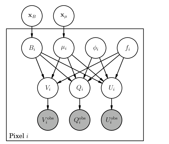
Figure 1: Graphical model representing the hierarchical Bayesian scheme that we used to analyze the set of Stokes signals in the quiet Sun. Open circles represent random variables (note that both model parameters and observations are considered as random variables), while the grey circle represents a measured quantity. The frame labeled “Pixel $i$” represents that everything inside the frame has to be repeated for all the observations. An arrow between two nodes illustrates dependency. The nodes that are outside the frame are the hyperparameters of the model and are common to all pixels.

Assuming that the weak-field approximation holds, the Stokes profiles can be explained with the set of parameters $\mbox{\boldmath$\theta$}=(B,\mu,f,\phi)$, where $B\in[0,\infty)$ is the magnetic field strength, $\mu\in[-1,1]$ refers to the cosine of the inclination angle of the magnetic field vector with respect to the line-of-sight, and $\phi\in[0,2\pi]$ is the azimuth of the magnetic field vector. Finally, $f\in[0,1]$ is the fraction of the resolution element that is filled with magnetic field, with the remaining $1-f$ fraction being field-free. Following (Landi Degl’Innocenti 1992), we simplify the model by assuming that the presence of a magnetic field does not affect Stokes $I$, so that it is the same in the magnetic and the non-magnetic fraction of the resolution element. All in all, the series expansion at first order in Stokes $V$ and second order in Stokes $Q$ and $U$ yields the following expressions for an arbitrary pixel $i$:

$$V_{i}(\lambda) =\alpha B_{i}\mu_{i}f_{i}\left(\frac{d{I}_{i}(\lambda)}{d\lambda}\right),$$

$$Q_{i}(\lambda) =\beta B_{i}^{2}(1-\mu_{i}^{2})f_{i}\cos 2\phi_{i}\left(\frac{d^{2}{I}_{i}(\lambda)}{d\lambda^{2}}\right),$$

$$U_{i}(\lambda) =\beta B_{i}^{2}(1-\mu_{i}^{2})f_{i}\sin 2\phi_{i}\left(\frac{d^{2}{I}_{i}(\lambda)}{d\lambda^{2}}\right),$$ (4)

where $\alpha=-4.67\times 10^{-13}\lambda_{0}^{2}\bar{g}$ and $\beta=-5.45\times 10^{-26}\lambda_{0}^{4}\bar{G}$ are constant that depend on the central wavelength of the spectral line and on the effective Landé factor, $\bar{g}$, and its equivalent for linear polarization, $\bar{G}$. Additionally, we have particularized the model parameters to the pixel of interest. As a requisite for the previous expressions to hold, we have to additionally assume that the magnetic field vector is constant along the line of sight in the formation region of the spectral line. A point that deserves a comment is the fact that the thermodynamic properties of the fraction $f$ of the pixel that generates the Stokes $Q$, $U$ and $V$ signals are usually not the same of the remaining $1-f$ fraction. In such a case, the simple approach followed in this paper cannot be applied and one has to be aware that there is some remaining information about the filling factor in the Stokes $I$ profile (e.g., Orozco Suárez et al. 2007a). However, a careful analysis of this more complicated case has to be carried out to avoid biasing the inferred values.

2.2 Hierarchical probabilistic model

The statistical model that we use in this paper to extract information from the observations is displayed in graphical form in Fig. 1. All the variables inside open circles are considered random variables, while those inside shaded circles are observations. The Stokes $Q$, $U$ and $V$ profiles of pixel $i$ of the $N$ available are explained using the set of variables $\{B_{i},\mu_{i},\phi_{f},f_{i}\}$ and the synthetic model of Eq. (4). For each pixel, the synthetic Stokes profiles are compared with the observed Stokes profiles using the appropriate model for the noise discussed in Sec. 2.3. The hierarchical character of the model comes from the fact that we make the prior distribution of the parameters of the model $\{B_{i},\mu_{i}\}$ with $i=1\ldots N$ depend on a set of parameters $\mathbf{x}_{B}$ and $\mathbf{x}_{\mu}$ that, lying outside the frame, are thus common to all pixels. This is one of the improvements brought by the hierarchical approach, in contrast to the previous work in Asensio Ramos (2009), where the priors were chosen to be uninformative.

We do not consider hierarchy in the azimuth and the filling. Concerning the azimuth, we do it because a simple statistical analysis of the $Q(\lambda)$ and $U(\lambda)$ signals yields that the azimuths are random in the quiet Sun. For this reason, we will not get much information from this parameters. This affirmation is based on several observations. For instance, a principal component analysis of the linear polarization signals in a large region of the quiet Sun shows exactly the same first few principal components in both $Q(\lambda)$ and $U(\lambda)$. As a consequence, the prior distribution is $p(\phi_{i})=(\phi_{\mathrm{max}}-\phi_{\mathrm{min}})^{-1}$, where $\phi_{\mathrm{min}}$ and $\phi_{\mathrm{max}}$ are the limits of the parameter. Concerning the filling factor, it is important to note that the application of the weak-field approximation to explain polarimetric signals coming from non-resolved structures is problematic because it is heavily degenerate with the other parameters. Consequently, we will not be able to extract relevant information from it. Instead of just making $f=1$ and assuming that the whole pixel is filled with a magnetic field, we consider it as a nuisance parameter that is integrated during the marginalization. Therefore, a priori $p(f_{i})=1$.

Following the standard Bayesian formulation of an inference problem, the solution has to be given in terms of the posterior distribution for all the parameters, that encodes all the information about the parameters of interest. We represent it as $p(\mathbf{B},\mbox{\boldmath$\mu$},\mbox{\boldmath$\phi$},\mathbf{f},\mathbf{x}_{B},\mathbf{x}_{\mu}|\mathbf{D})$, where $\mathbf{D}=\{D_{1},D_{2},\ldots,D_{N}\}$ and $D_{i}=\{I_{\mathrm{obs}}^{i}(\lambda),Q_{\mathrm{obs}}^{i}(\lambda),U_{\mathrm{obs}}^{i}(\lambda),V_{\mathrm{obs}}^{i}(\lambda)\}$ refers to the set of Stokes profiles for $i$-th pixel of the set of $N$ observed pixels. Likewise, $\mathbf{B}$, $\mu$, $\phi$ and $\mathbf{f}$ are vectors that contain all the parameters of the model for all the pixels, while $\mathbf{x}_{B}$ and $\mathbf{x}_{\mu}$ are the set of hyperparameters that are used to describe the priors for the physical parameters of interest (see Sect. 2.4). Applying the Bayes theorem, the posterior can be written as:

$$p(\mathbf{B},\mbox{\boldmath$\mu$},\mbox{\boldmath$\phi$},\mathbf{f},\mathbf{x}_{B},\mathbf{x}_{\mu}|\mathbf{D})=\frac{p(\mathbf{D}|\mathbf{B},\mbox{\boldmath$\mu$},\mbox{\boldmath$\phi$},\mathbf{f},\mathbf{x}_{B},\mathbf{x}_{\mu})p(\mathbf{B},\mbox{\boldmath$\mu$},\mbox{\boldmath$\phi$},\mathbf{f},\mathbf{x}_{B},\mathbf{x}_{\mu})}{p(\mathbf{D})},$$ (5)

where $p(\mathbf{D})$ is the evidence, a normalization constant that is unimportant in our analysis. In the previous equation, $\mathcal{L}=p(\mathbf{D}|\mathbf{B},\mbox{\boldmath$\mu$},\mbox{\boldmath$\phi$},\mathbf{f},\mathbf{x}_{B},\mathbf{x}_{\mu})$ is the likelihood, which measures the ability of a set of parameters to fit the observations and that we will discussed in Sec. 2.3. Likewise, $p(\mathbf{B},\mbox{\boldmath$\mu$},\mbox{\boldmath$\phi$},\mathbf{f},\mathbf{x}_{B},\mathbf{x}_{\mu})$ is the prior distribution, that we elaborate in Sec. 2.4.

2.3 Likelihood

The likelihood of Eq. (5) can be simplified in two steps. First, it is clear from Eq. (4) and Fig. 1 that the synthetic Stokes profiles (and, consequently, the likelihood) do only depend on the set of variables $\{\mathbf{B},\mbox{\boldmath$\mu$},\mbox{\boldmath$\phi$},\mathbf{f}\}$, and not on the hyperparameters $\mathbf{x}_{B},\mathbf{x}_{\mu}$. Therefore, the simplification $p(\mathbf{D}|\mathbf{B},\mbox{\boldmath$\mu$},\mbox{\boldmath$\phi$},\mathbf{f},\mathbf{x}_{B},\mathbf{x}_{\mu})=p(\mathbf{D}|\mathbf{B},\mbox{\boldmath$\mu$},\mbox{\boldmath$\phi$},\mathbf{f})$ applies. Second, we make the assumption that the measurements for all the pixels are statistically independent, so that the likelihood factorizes as:

$$\mathcal{L}=\prod_{i=1}^{N}\mathcal{L}_{i}=\prod_{i=1}^{N}p(D_{i}|B_{i},\mu_{i},\phi_{i},f_{i}).$$ (6)

The analytical expression for each individual likelihood depends on the noise statistics. If the observations are perturbed with Gaussian noise of variance $\sigma_{n}^{2}$ (we assume for simplicity that there is no correlation between different wavelengths or different Stokes profiles, although it can be easily generalized to the case in which such correlation matrix is known), the likelihood for a single pixel is described by a Gaussian with zero mean and variance $\sigma_{n}^{2}$. Making everything explicit, each likelihood can be written as

$$\mathcal{L}_{i} =p(D_{i}|B_{i},\mu_{i},\phi_{i},f_{i})=(2\pi)^{-M/2}{\sigma_{n}}^{-M}$$

$$\times\exp\Bigg{\{}-\frac{1}{2{\sigma_{n}}^{2}}\sum_{j=1}^{M}\left[V_{i}(\lambda_{j})-\alpha_{j}B_{i}\mu_{i}f_{i}\left(\frac{d{I}_{i}(\lambda)}{d\lambda}\right)_{j}\right]^{2}$$

$$-\frac{1}{2{\sigma_{n}}^{2}}\sum_{j=1}^{M}\left[Q_{i}(\lambda_{j})-\beta_{j}B_{i}^{2}(1-\mu_{i}^{2})f_{i}\cos 2\phi_{i}\left(\frac{d^{2}{I}_{i}(\lambda)}{d\lambda^{2}}\right)_{j}\right]^{2}$$

$$-\frac{1}{2{\sigma_{n}}^{2}}\sum_{j=1}^{M}\left[U_{i}(\lambda_{j})-\beta_{j}B_{i}^{2}(1-\mu_{i}^{2})f_{i}\sin 2\phi_{i}\left(\frac{d^{2}{I}_{i}(\lambda)}{d\lambda^{2}}\right)_{j}\right]^{2}\Bigg{\}}$$ (7)

where $M$ is the number of wavelength points of each observed Stokes profiles. Further simplications in the notation are shown in Appendix A.

2.4 Priors

The prior distribution encodes all the a-priori information that we know about the parameters. Instead of using fixed prior distributions, in a hierarchical approach we make them depend on additional parameters (termed hyperparameters), that are inserted in the Bayesian inference. The dependencies can be easily extracted from the graphical model of Fig. 1, so that the full prior distribution can be factorized according to:

$$p(\mathbf{B},\mbox{\boldmath$\mu$},\mbox{\boldmath$\phi$},\mathbf{f},\mathbf{x}_{B},\mathbf{x}_{\mu}) =p(\mathbf{B}|\mathbf{x}_{B})p(\mbox{\boldmath$\mu$}|\mathbf{x}_{\mu})p(\mathbf{x}_{B})p(\mathbf{x}_{\mu})p(\mathbf{f})p(\mbox{\boldmath$\phi$})$$ (8)

which can be even further simplified by assuming that the prior for the parameters of each pixel are independent, so that

$$p(\mathbf{B},\mbox{\boldmath$\mu$},\mbox{\boldmath$\phi$},\mathbf{f},\mathbf{x}_{B},\mathbf{x}_{\mu}) =p(\mathbf{x}_{B})p(\mathbf{x}_{\mu})$$

$$\times\prod_{i=1}^{N}p(B_{i}|\mathbf{x}_{B})p(\mu_{i}|\mathbf{x}_{\mu})p(\phi_{i})p(f_{i}).$$ (9)

Note that the prior for the azimuth is left non-hierarchical and chosen to be uniform in the interval $[0,\pi]$, while that of the filling factor is also non-hierarchical and uniform in the interval $[0,1]$. Given the inherent 180^∘ ambiguity in the azimuth in the line-of-sight of the Zeeman effect, we decided to limit the solution to only one of the solutions. This is motivated by two reasons. First, once the solution is obtained, we immediately know the ambiguous solution. Second, working with multimodal distributions is problematic and dealing with the two ambiguous solutions offers nothing new to the hierarchical analysis.

Using previous experience (Asensio Ramos & Arregui 2013; Asensio Ramos 2014), we have decided to use very simple prior distributions for the model parameters, chosen based on the conditions: i) they are mathematically simple but flexible enough to adapt during the inference and, ii) they naturally fulfill the physical constraints. Note that the assumed prior is also an inherent part of the model, at the same level as the generative model. The fact that the hyperparameters are random variables, will allow us to use these simple prior distributions to generate quite complex global distributions.

Given that $B\in[0,\infty)$, it makes sense to use a log-normal prior for this lower-bounded parameter:

$$p(B_{i}|\mathbf{x}_{B})=\mathrm{LN}(B_{i};\alpha_{B},\beta_{B})=\frac{1}{\sqrt{2\pi}\beta_{B}B_{i}}\exp\left[-\frac{(\log B_{i}-\alpha_{B})^{2}}{2\beta_{B}^{2}}\right],$$ (10)

where $\alpha_{B}\in(-\infty,\infty)$ and $\beta_{B}>0$ are the hyperparameters. In the notation used in Fig. 1, we have that $\mathbf{x}_{B}=(\alpha_{B},\beta_{B})$. One of the main properties of this prior is that, independently of the value of $\alpha$ and $\beta$, the probability of having $B=0$ is zero. Domínguez Cerdeña et al. (2006b) and Sánchez Almeida (2007) pointed out that, when the field strength is weak, the field becomes very tangled and random. Consequently, it is very improbable that the three components of the magnetic field vector become zero simultaneously, something that is naturally fulfilled by the prior.

Concerning the cosine of the heliocentric angle, is is limited to the bounded intervals $\mu\in[-1,1]$. A natural distribution for such bounded parameter which is able to take a large variety of shapes is the scaled Beta prior:

$$p(\mu_{i}|\mathbf{x}_{\mu}) =\mathrm{Beta}(\mu_{i};\alpha_{\mu},\beta_{\mu},a,b)$$

$$=\frac{(b-a)^{1-\alpha_{\mu}-\beta_{\mu}}}{B(\alpha_{\mu},\beta_{\mu})}(\mu_{i}-a)^{\alpha_{\mu}-1}(b-\mu_{i})^{\beta_{\mu}-1},$$ (11)

with $\alpha_{\mu}>0$ and $\beta_{\mu}>0$ the hyperparameters, $B(\alpha_{\mu},\beta_{\mu})=\Gamma(\alpha_{\mu})\Gamma(\beta_{\mu})/\Gamma(\alpha_{\mu}+\beta_{\mu})$ the Beta function (Abramowitz & Stegun 1972) and $a=-1$ and $b=1$ are the limits of the interval. The hyperparameters will then be $\mathbf{x}_{\mu}=(\alpha_{\mu},\beta_{\mu})$.

2.4.1 Priors for hyperparameters

Given that we have introduced four hyperparameters in the Bayesian inference, we have to use priors for them. Concerning the prior for the magnetic field strength, we use the standard approach and set a Jeffreys’ prior for the scale parameter $\beta_{B}$, while setting an uniform prior for the location parameter $\alpha_{B}$. For the Beta prior for $\mu$, leaving uniform priors for the hyperparameters of a Beta prior will surely lead to an improper posterior (the integral of the posterior becomes infinity). Gelman et al. (2003) suggest to use flat priors on the variables

$$\bar{\mu}=\frac{\alpha_{\mu}b+\beta_{\mu}a}{\alpha_{\mu}+\beta_{\mu}},\qquad\nu=(\alpha_{\mu}+\beta_{\mu})^{-1/2},$$ (12)

which are the mean of the distribution and inverse square root of the sample size. Using the Jacobian of the transformation from $(\bar{\mu},\nu)$ to $(\alpha_{\mu},\beta_{\mu})$, the prior becomes $p(\alpha_{\mu},\beta_{\mu})=(\alpha_{\mu}+\beta_{\mu})^{-5/2}$.

2.4.2 Marginal posterior

From the previous considerations, we can obtain the full posterior by multiplying the likelihood and the priors, yielding:

$$p(\mathbf{B}, \mbox{\boldmath$\mu$},\mbox{\boldmath$\phi$},\mathbf{f},\mathbf{x}_{B},\mathbf{x}_{\mu}|\mathbf{D})\propto p(\mathbf{x}_{B})p(\mathbf{x}_{\mu})$$

$$\times\prod_{i=1}^{N}p(D_{i}|B_{i},\mu_{i},\phi_{i},f_{i})p(B_{i}|\mathbf{x}_{B})p(\mu_{i}|\mathbf{x}_{\mu})p(\phi_{i})p(f_{i}).$$ (13)

The marginalization of all the individual parameters of the model for each pixel will yield

$$p(\mathbf{x}_{B},\mathbf{x}_{\mu}|\mathbf{D}) \propto p(\mathbf{x}_{B})p(\mathbf{x}_{\mu})$$

$$\times\prod_{i=1}^{N}\Bigg{[}\int\mathrm{d}B_{i}\,\mathrm{d}\mu_{i}\,\mathrm{d}\phi_{i}\,\mathrm{d}f_{i}p(D_{i}|B_{i},\mu_{i},\phi_{i},f_{i})$$

$$\times p(B_{i}|\mathbf{x}_{B})p(\mu_{i}|\mathbf{x}_{\mu})p(\phi_{i})p(f_{i})\Bigg{]}.$$ (14)

We finally note that either the integral over $\phi_{i}$ or over $f_{i}$ can be carried out analytically when using flat priors. This reduces the dimensionality of the problem but is less general in case one wants to use other priors. The expression for the marginal likelihood when integrating $f_{i}$ is shown in App. B.

Figure 2: Inferred values for the hyperparameters of the priors for $B$ (upper panels) and $\mu$ (lower panels). The first and third columns show the last 3000 samples of the Markov chains, while the second and fourth show the associated histograms. The last column displays the Monte Carlo inferred distribution of $B$ and $\mu$ taking into account the observations. These results are obtained with 5% of the FOV, although they remain the same as far as $\sim$0.5% of the field of view is included in the analysis.

2.5 Inference

Given the Stokes profiles observed at $N$ pixels, the posterior becomes a $4N+4$-dimensional distribution. It is usual to apply MCMC methods to carry out the sampling from the posterior, but the large dimensionality and the hierarchical character of the probabilistic model preclude an efficient solution even using advanced techniques like Hamiltonian Monte Carlo methods Duane et al. (1987). For this reason, we carry out an efficient approximation for the marginal posterior of Eq. (14). The idea is based on carrying out the inference of each individual pixel independently using common priors $p(B_{i})$ and $p(\mu_{i})$, and then reconstructing back the results using importance sampling, similar to the approach used recently by Hogg et al. (2010) and Brewer & Elliott (2014):

$$p(\mathbf{x}_{B},\mathbf{x}_{\mu}|\mathbf{D}) \propto p(\mathbf{x}_{B})p(\mathbf{x}_{\mu})$$

$$\times\prod_{i=1}^{N}\Bigg{[}\int\mathrm{d}B_{i}\,\mathrm{d}\mu_{i}\,\mathrm{d}\phi_{i}\,\mathrm{d}f_{i}p(D_{i}|B_{i},\mu_{i},\phi_{i},f_{i})$$

$$\times\frac{p(B_{i}|\mathbf{x}_{B})p(\mu_{i}|\mathbf{x}_{\mu})}{p(\mathbf{B})p(\mbox{\boldmath$\mu$})}p(B_{i})p(\mu_{i})p(\phi_{i})p(f_{i})\Bigg{]}.$$ (15)

If we carry out a sampling of the posterior for each individual pixel with the common priors, we can estimate the integral using:

$$p(\mathbf{x}_{B},\mathbf{x}_{\mu}|\mathbf{D}) \propto p(\mathbf{x}_{B})p(\mathbf{x}_{\mu})\prod_{i=1}^{N}\mathbb{E}\Bigg{[}\frac{p(B_{i}|\mathbf{x}_{B})p(\mu_{i}|\mathbf{x}_{\mu})}{p(\mathbf{B})p(\mbox{\boldmath$\mu$})}\Bigg{]},$$ (16)

where $\mathbb{E}(x)$ refers to the expectation value, which is taken with respect to the pixel marginal posterior. Our calculations are done with flat common priors, with a large support for the prior for the magnetic field strength to ensure that it does not affect the computation of the hierarchical prior.

Summarizing, a standard MCMC sampling method is used to sample from the posterior of each pixel and these samples are stored. For computational reasons, we only store 100 samples, which is enough to get a robust final result. Then, we sample from the marginal posterior of Eq. (16) using again an MCMC. To this end, we compute, at each iteration, the expectation inside the product with the stored samples .

3 Results

The previous hierarchical model is applied to the quiet Sun observations presented by Lites et al. (2008) using Hinode (Kosugi et al. 2007) with the spectropolarimeter of the solar optical telescope(SOT/SP; Lites et al. 2001). We focus on the Fe i line at $\lambda_{0}=6302.5$ Å, which has $\bar{g}=2.5$ and $\bar{G}=6.25$. Even though the dimensions of the map are enormous ($2048\times 1024$ pixels, which cover an area of $300^{\prime\prime}\times 160^{\prime\prime}$ on the Sun), we have verified that the line-of-sight can be assumed to be roughly normal to the surface. Therefore, $\mu_{i}$ in our model will always represents the cosine of the angle that the magnetic field vector makes with the vertical.

We estimate the noise level in the continuum to be roughly the same for all the Stokes parameters and equal to $\sigma_{n}\sim 1.1\times 10^{-3}$ in units of the continuum intensity (e.g., Lites et al. 2008). We only keep pixels that have signals in Stokes $Q$, $U$ or $V$ larger than 4.5 times the noise level in the continuum, so filtering out pixels that only contain noise. After this filtering, only 27% ($\sim$560000 pixels) of the FOV is considered. When computing Eq. (16), we test that the results are insensitive to the exact value of $N$ provided that $N\gtrsim 10000$.

We display in Fig. the final results for $N=120000$ pixels. The upper row shows the results for the hyperparameters of the magnetic field strength, while the lower panels shows the final results for the hyperparameters of the cosine of the magnetic field inclination with respect to the line-of-sight. The first and third columns show 3000 samples from the Markov chains for the four hyperparameters, while the second and fourth columns display their histograms. They are the marginal posteriors for the four hyperparameters. Note that they have the well-defined values $\alpha_{B}=4.75\pm 0.01$, $\beta_{B}=0.52\pm 0.01$, $\alpha_{\mu}=2.63\pm 0.02$ and $\beta_{\mu}=2.40\pm 0.02$. Using these values and the properties of the log-normal distribution, we find $\langle B\rangle=132\pm 1$ G and $\sqrt{\langle B^{2}\rangle}=151\pm 1$ G, in agreement with previous results, which were obtained following different approaches (e.g., Trujillo Bueno et al. 2004; Martínez González 2006; Domínguez Cerdeña et al. 2006b).

Using these results, there are two ways to compute the global magnetic properties of the analyzed pixels, i.e., the distribution of field strengths and inclinations in the whole FOV analyzed that would be compatible with noise and degeneracies in each pixel. The first one is to use what is known as the type-II maximum likelihood approximation. To this end, we simply evaluate the priors defined in §2.4 at the most probable values of their parameters, obtained from the peaks on Fig. 2. The second way, that is the one we use for producing the plots on the last column of Fig. 2, is to compute the following Monte Carlo estimation of the marginalization of the hyperparameters from the priors using $N_{s}$ samples:

$$\langle p(B|D)\rangle =\frac{1}{N_{s}}\sum_{i=1}^{N_{s}}\mathrm{LN}(B;\alpha_{B}^{i},\beta_{B}^{i})$$

$$\langle p(\mu|D)\rangle =\frac{1}{N_{s}}\sum_{i=1}^{N_{s}}\mathrm{Beta}(\mu;{\alpha_{\mu}}^{i},{\beta_{\mu}}^{i},-1,1).$$ (17)

Given that the marginal posterior distributions for the hyperparameters are very well defined, the type-II maximum likelihood and the Monte Carlo estimation essentially overlap. The distributions in the rightmost panels of Fig. 2 are calculated taking into account the information from $N=120000$ pixels and their uncertainties in the inferred parameters and combining them in one distribution. This includes the effect of noise, degeneracies and any other uncertainty. They constitute the main result of this paper and have to be confronted with previous studies. Because of the presence of noise and degeneracies, these distributions broaden with respect to the true ones. Observations with a better signal-to-noise ratio would reduce this broadening but would never reduce the broadening produced by the inherent degeneracies of the model.

Figure 3: Marginal posterior for the magnetic field strength when we measure different values of the product $fB$ (indicated in the legend) with an uncertainty of 0.5 Mx cm^-2. The fact that we assume a flat prior for $f$ induces that the most probable value for $B$ is very small, close to what one would measure assuming $f=1$. The extended tail is produced by the small possible values of $f$.

The distribution for the magnetic field strength is quite similar to previous results. This means that the effect of noise and degeneracies in earlier works with histogramming the maximum-likelihood estimations was small. The reason for that is that the amount of hG fields is so large that the influence of the tails induced by the presence of noise and degeneracies is not very important. Therefore, just picking up the mode of the distribution results in a good estimation of the global distribution of magnetic field strengths. The good point of the Bayesian approach is that we verify that taking the mode seems to be a good strategy. Fields are in the hG regime, with the distribution peaking around 85 G. With the observed data and our current analysis, the field strength is below 275 G with 95% credibility. Certainly, this should not be confused with the fraction of pixels having these fields, which would be a frequentist Because we are including the filling factor and the inclination of the field into the inference, we are able to extract values of the magnetic field strength, even though we are working in the weak-field regime. In fact, we are considering all possible values of the filling factor and inclination that are compatible with the observations for each individual pixel. Even in the extreme case that only the amplitude of circular polarization is available (a map of magnetic flux density), it is still possible to give inferences about the magnetic field strength. If we observe a certain magnetic flux density, $\Phi_{\mathrm{obs}}$, and we model it with the simple expression $\Phi=Bf\mu$, the marginal posterior for the field strength is given by

$$p(B|\Phi)\propto p(B)\int_{0}^{1}\mathrm{d}f\int_{-1}^{1}\mathrm{d}\mu\exp\left[-\frac{\left(\Phi_{\mathrm{obs}}-Bf\mu\right)^{2}}{2\sigma_{n}^{2}}\right],$$ (18)

where we have assumed flat priors for $\mu$ in the interval $[-1,1]$ and $f$ in the interval $[0,1]$. For a noise with standard deviation $\sigma_{n}=0.5$ Mx cm^-2, the marginal posteriors for a few measured values of $\Phi$ are displayed in Fig. 3. According to this result, since the prior distributions for $f$ and $\mu$ are assumed to be flat, the peak of the distribution or marginal maximum a-posteriori (MMAP) value of the magnetic field is small (close to $\Phi$), with a very long tail towards higher values.

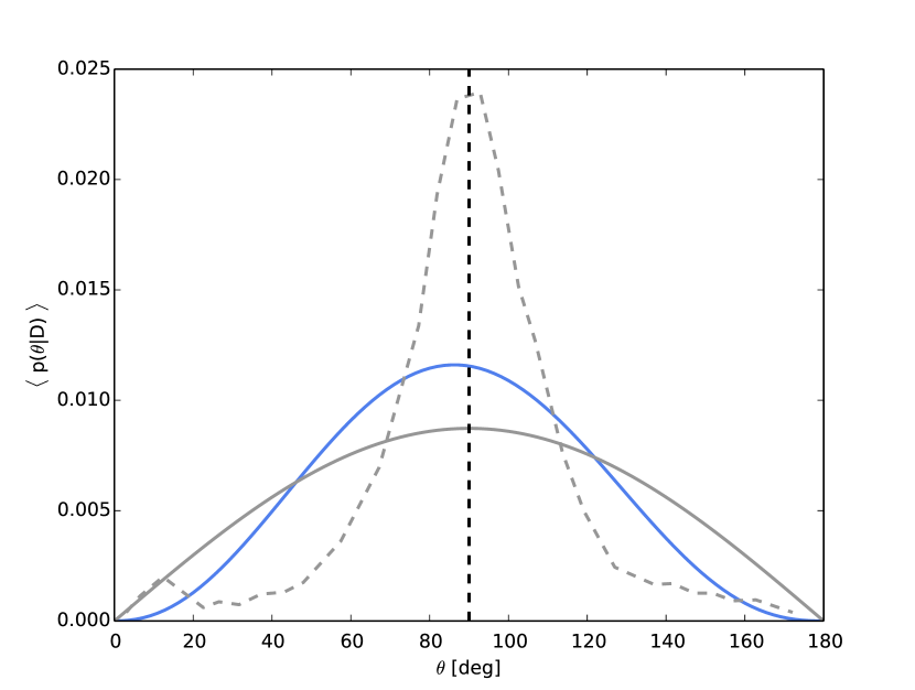
Figure 4: Inferred global distribution of inclinations from the data (blue), compared with the expected distribution of inclinations for an isotropic vector field (solid gray). For comparison, we have overplotted in dashed gray line the distribution inferred by Bellot Rubio & Orozco Suárez (2012), which we obtained by scanning the original figure. For reference, the vertical dashed line indicates purely horizontal fields.

Concerning the magnetic field inclination, a simple change of variables can be used to transform the distribution for $\mu$ shown in the lower panel of the last column of Fig. 2 into a distribution for the inclination of the field, $\theta$. Starting from $p_{\mu}(\mu)$, the distribution $p_{\theta}(\theta)$ in terms of $\theta$ is given by

$$p_{\theta}(\theta)=p_{\mu}(\mu=\cos\theta)|\sin\theta|,$$ (19)

where we have made explicit that the distributions are different. Applying this change of variables, we end up with the distribution displayed in blue in Fig. 4. For comparison, we show the distribution associated with an isotropic field, which has $p_{\mu}(\mu)=1/2$ or, equivalently, $p_{\theta}(\theta)=\sin(\theta)/2$. Additionally, we also display the distribution of inclinations obtained by Bellot Rubio & Orozco Suárez (2012) in dashed gray lines. The distribution of fields is close to $\langle p(\theta|D)\rangle\propto\sin^{2}\theta$, although with a slight skewness towards fields pointing downwards ($\mu<0$, equivalently, $0^{\circ}<\theta<90^{\circ}$). Figure 4 shows that there are slightly more highly-inclined fields and slightly less highly-vertical fields than what one would expect for an isotropic field. In numbers, the inferred distribution contains $\sim$80% of the fields in the very inclined regime ($45^{\circ}<\theta<135^{\circ}$), while the isotropic distribution contains $1/\sqrt{2}\sim 70$% in this regime.

Our new result is to be preferred over our previous result in Asensio Ramos (2009), although with some caveats because we are using a simpler model for explaining the polarimetric signals. In Asensio Ramos (2009), the peak in 40^∘ and 140^∘ is a consequence of the fact that the polarimetric signal is very weak, so only the polarity can be estimated in many pixels. As a consequence, the median value that we used to summarize the marginal posteriors peak around the center of the intervals $[0^{\circ},90^{\circ}]$ and $[90^{\circ},180^{\circ}]$, as already explained in Asensio Ramos (2009). Additionally, given the scarcity of information, they also used the cumulative distribution to give a hint that the field seems to be close to isotropic for the the pixels with the weakest signals. In this updated work, we take these large uncertainties into account and extract the global distribution of inclinations, under the assumption that all the pixels share a common probability distribution. Note that, even though fields close to 90^∘ are favored, the distribution is very close to isotropic. Finally, as compared with the distribution inferred previously by Bellot Rubio & Orozco Suárez (2012) from the same data, it is obvious that our results point towards a much more quasi-isotropic distribution, in a way similar to the results of Asensio Ramos (2009) and Stenflo (2010).

Even though the presence of noise complicates the inference of the field inclination, our results are certainly less affected than other previous results for one reason: we compute all field inclinations that are compatible with the observations for each individual pixel, together with their associated probability. Then, these distributions are used to estimate the global field inclination distribution, fully taking into account the presence of uncertainties. If the noise variance is decreased in future observations, the ensuing posterior distributions for each individual pixel will certainly be narrower, resulting in more informative global field inclination distributions.

4 Conclusions

This paper presents our first attempt to infer global distributions of magnetic field strength and inclinations from spectropolarimetric data taking fully into account all the degeneracies. To this end, we applied a Bayesian hierarchical model. The difficulty of the statistical model forced us to use the weak-field approximation simplified model to explain the polarimetric signals. Although simplified, this model captures a large fraction of the behavior that is explained by more complicated models.

Our results indicate that the magnetic field strength has to be weak, below 275 G with 95% credibility. This is a direct consequence of the fact that we consider that all values of the filling factor in the interval $[0,1]$ are equiprobable a-priori. Concerning the distribution of field inclinations, we find a rather quasi-isotropic distribution, roughly proportional to $\sin^{2}\theta$.

In the future, we plan to extend our hierarchical approach to more complicated models for the Stokes profiles. The main obstacle resides on the potentially high dimensionality of the probabilistic model given that more complicated models need a larger number of free parameters.

Appendix A Likelihood

The likelihood of Eq. (7) can be written in a more simplified form showing that only 8 numbers per pixel are needed from the observations. Regrouping terms, the definition of the likelihood of Eq. (7) can be simplified to read:

$$p(D_{i}|B_{i},\mu_{i},\phi_{i},f_{i}) =(2\pi)^{-M/2}{\sigma_{n}}^{-M}\exp\Bigg{\{}-\frac{1}{2{\sigma_{n}}^{2}}\left[C_{V1i}+B_{i}^{2}\mu_{i}^{2}f_{i}^{2}C_{V2i}-B_{i}\mu_{i}f_{i}C_{V3i}\right.$$

$$+C_{Q1i}+B_{i}^{4}(1-\mu_{i}^{2})^{2}f_{i}^{2}\cos^{2}2\phi_{i}C_{Q2i}-B_{i}^{2}(1-\mu_{i}^{2})f_{i}\cos 2\phi_{i}C_{Q3i}$$

$$+\left.C_{U1i}+B_{i}^{4}(1-\mu_{i}^{2})^{2}f_{i}^{2}\sin^{2}2\phi_{i}C_{U2i}-B_{i}^{2}(1-\mu_{i}^{2})f_{i}\sin 2\phi_{i}C_{U3i}\right]\Bigg{\}},$$ (20)

where

$$C_{V1i}= \sum_{j=1}^{M}V_{i}^{2}(\lambda_{j}),\qquad C_{V2i}=\alpha^{2}\sum_{j=1}^{M}\left(\frac{d{I}_{i}(\lambda)}{d\lambda}\right)^{2}_{j},\qquad C_{V3i}=2\alpha\sum_{j=1}^{M}V_{i}(\lambda_{j})\left(\frac{d{I}_{i}(\lambda)}{d\lambda}\right)_{j}$$

$$C_{Q1i}= \sum_{j=1}^{M}Q_{i}^{2}(\lambda_{j}),\qquad C_{Q2i}=\beta^{2}\sum_{j=1}^{M}\left(\frac{d^{2}{I}_{i}(\lambda)}{d\lambda^{2}}\right)^{2}_{j},\qquad C_{Q3i}=2\beta\sum_{j=1}^{M}Q_{i}(\lambda_{j})\left(\frac{d^{2}{I}_{i}(\lambda)}{d\lambda^{2}}\right)_{j}$$

$$C_{U1i}= \sum_{j=1}^{M}U_{i}^{2}(\lambda_{j}),\qquad C_{U2i}=\beta^{2}\sum_{j=1}^{M}\left(\frac{d^{2}{I}_{i}(\lambda)}{d\lambda^{2}}\right)^{2}_{j},\qquad C_{U3i}=2\beta\sum_{j=1}^{M}U_{i}(\lambda_{j})\left(\frac{d^{2}{I}_{i}(\lambda)}{d\lambda^{2}}\right)_{j}.$$ (21)

Note that $C_{Q2i}=C_{U2i}$, which reduces the number of quantities needed to describe the information that we need from the Stokes profiles to 8.

Appendix B Likelihood integrating the filling factor

Given that the likelihood is factorizable and Gaussian, the filling factor can be marginalized from the posterior analytically. This is possible if we use a flat prior for this parameter, so that:

$$\int\mathrm{d}f_{i}p(D_{i}|B_{i},\mu_{i},\phi_{i},f_{i})p(f_{i})=\frac{\sqrt{\pi}}{2\sqrt{C}}\exp\left[-A+\frac{B^{2}}{4C}\right]\left[\mathrm{erf}\left(\frac{B}{2\sqrt{C}}\right)-\mathrm{erf}\left(\frac{B-2C}{2\sqrt{C}}\right)\right],$$ (22)

where the quantities $A$, $B$ and $C$ are defined as:

$$A =C_{V1i}+C_{Q1i}+C_{U1i}$$

$$B =B_{i}\mu_{i}C_{V3i}+B_{i}^{2}(1-\mu_{i}^{2})\left(\cos 2\phi_{i}C_{Q3i}+\sin 2\phi_{i}C_{U3i}\right)$$

$$C =B_{i}^{2}\mu_{i}^{2}C_{V2i}+B_{i}^{4}(1-\mu_{i}^{2})^{2}\left(\cos^{2}2\phi_{i}C_{Q2i}+\sin^{2}2\phi_{i}C_{U2i}\right)$$ (23)