Tests for Time Series of Counts Based on the Probability Generating Function

Abstract

We propose testing procedures for the hypothesis that a given set of discrete observations may be formulated as a particular time series of counts with a specific conditional law. The new test statistics incorporate the empirical probability generating function computed from the observations. Special emphasis is given to the popular models of integer autoregression and Poisson autoregression. The asymptotic properties of the proposed test statistics are studied under the null hypothesis as well as under alternatives. A Monte Carlo power study on bootstrap versions of the new methods is included as well as real–data examples.

62M10, 62F03, 62F40

1 Introduction

Let $\{Y_{t}\}_{t\in\mathbb{N}}$ denote a time series of counts for which, conditionally on the past, the corresponding stochastic structure is fully specified by a family of laws indexed by a certain parameter. Such models include the model of integer autoregression (INAR) as well as the integer autoregressive conditionally heteroscedastic (INARCH) model. These two models have received enormous attention in the past as they are known to fit empirical data in diverse areas of application. The objective here is to construct goodness–of–fit (GOF) statistics for distributional assumptions regarding these count time series models. In the classical (continuous type) framework of time–series models, this aspect of modelling has drawn considerable attention recently; see [1, 2, 3, 4, 5]. The standard approach in constructing GOF tests is to estimate the corresponding density or distribution function and thereby construct versions of the Kolmogorov–Smirnov, Cramér–von Mises and Bickel–Rosenblatt statistics. However, there is also the alternative route of employing empirical transforms, such as the empirical Laplace transform and the empirical characteristic function, to the same problem. This idea was first put forward by Epps [6] and has recently been followed by Cuesta Albertos et al. [7], Ghosh [8], and Klar et al. [9].

Now turning to count data, Fokianos and Neumann [10] have considered GOF tests for the regression function in parametric versions of count time series. Here we consider another aspect of such series, namely the aspect of correctly specifying the conditional distribution of observations. In doing so we employ the aforementioned approach of empirical transforms and use marginal quantities by integrating up with respect to the conditioning argument in a spirit analogous to that in [11]. Specifically, the test statistics comes in the form of a weighted L2–type distance between a nonparametric estimate of the marginal probability generating function of the observations and a semiparametric estimate of the same quantity imposed by the model. Recall that if $Y$ is an arbitrary integer–valued random variable then its probability generating function (PGF) is defined as $g_{Y}(u)=\mathbb{E}[u^{Y}],\ u\in[0,1]$.

The remainder of this paper runs as follows. In Section 2 we specify the time series and the GOF problems considered, and construct the corresponding test statistics for the first order models. Computational issues are addressed in Section 3. In Section 4 the asymptotic properties of these statistics are studied both under the null hypothesis as well as under alternatives. Corresponding proofs are postponed to the appendix. In Section 5 we propose estimators for the parameters involved in our test statistics and suggest bootstrap versions of the new tests. Possible generalization of our approach to models of higher order is described in Section 6. In Section 7 we report the results on a Monte Carlo study, and the article concludes with some real data examples in Section 8.

2 Test statistics

Let ${\cal{I}}_{t}$ be the information set available at time $t$, i.e., ${\cal{I}}_{t}=\sigma\{Y_{s},\ s\leq t\}$ is a $\sigma$-field generated by the past values of the series $\{Y_{t}\}_{t\in\mathbb{N}}$. We assume that the conditional distribution of $Y_{t}$ given ${\cal{I}}_{t-1}$ can be described using a specific (cumulative) distribution function $F$ depending on ${\cal{I}}_{t-1}$ and also on an unknown parameter $\vartheta$ in the following way:

$$Y_{t}|\>{\cal{I}}_{t-1}\sim F(\cdot;{\cal{I}}_{t-1},\vartheta),$$ (1)

where $X\sim F(\cdot;\cdot,\cdot)$ is interpreted as ‘the random variable $X$ has $F(\cdot;\cdot,\cdot)$ as its distribution function’.

There exist two main classes of models that may be formulated in this way: The INAR model and INARCH model, both admitting several specifications and generalizations. We start with the most basic formulations.

(i) INAR model: For the INAR(1) model (see [12, 13, 14]) eqn. (1) is specified as

$$Y_{t}|\>{\cal{I}}_{t-1}\sim{\cal{B}}(Y_{t-1},p)\ast G_{\varepsilon},$$ (2)

where $\ast$ denotes convolution, ${\cal{B}}(\nu,p)$ is a binomial distribution with parameter $(\nu,p)$ and $G_{\varepsilon}$ is a distribution.More specifically the INAR(1) model can be constructed as

$$Y_{t}=\sum_{i=1}^{Y_{t-1}}U_{t,i}+\varepsilon_{t},\quad t=1,\ldots,$$ (3)

where $U_{1,1},\ldots$ are independent binary random variables such that $P(U_{t,i}=1)=p,\,P(U_{t,i}=0)=1-p,$ $p\in(0,1)$, and such that $U_{t,1},U_{t,2},\dots$ are independent of $Y_{t-1}$ and $\varepsilon_{t}$. The variables $\varepsilon_{t},\,t=1,\ldots$ are i.i.d. discrete nonnegative with distribution function $G_{\varepsilon}$ and PGF $g_{\varepsilon}(u)$ with finite variance such that $\varepsilon_{t}$ is independent of $Y_{t-1}$.

Generalizations of the INAR(1) to higher order models were proposed, see [15, 16], while a related review article is [17].

Specific instances of INAR(1) result when $G_{\varepsilon}$ is known to belong to a family of distributions ${\cal{G}}_{\Theta}$, the most popular case being when ${\cal{G}}_{\Theta}$ is the Poisson family, in which case $\vartheta=(p,\theta)^{\prime}$ with $\theta\in\Theta=(0,\infty)$ denoting the Poisson parameter. In fact, the property that the marginal distribution of the observations is from the same family as the distribution of innovations $\varepsilon_{t}$ characterizes the Poisson law in the context of INAR models. Wei$\upbeta$ [18] however points out that both the Negative Binomial as well as Consul’s generalized Poisson distribution may well serve as marginal laws under INAR models, particularly in view of overdispersed data. (In fact the set of all possible marginal laws coincides with the family of discrete self–decomposable distributions). Under the same type of data Pavlopoulos and Karlis [19] suggest a Poisson mixture for the innovation distribution, while Barczy et al. [20] entertain the idea of an INAR model with Poisson innovations, but containing outliers in the innovation distribution. Hence, and since under a fixed INAR model the law of the innovations uniquely determines the conditional as well as the marginal law of the observations, there is a clear need for GOF procedures in order to correctly identify the innovation distribution $G_{\varepsilon}$.

(ii) INARCH model: The INARCH(1) model is specified by (1) with

$$Y_{t}|\>{\cal{I}}_{t-1}\sim\mathsf{Po}(\lambda_{t}),\quad\lambda_{t}=r(Y_{t-1};\vartheta)$$ (4)

where $\mathsf{Po}(\lambda_{t})$ denotes Poisson distribution with parameter $\lambda_{t}$ , and $r(\cdot;\cdot)$ belongs to a specific parametric family of functions $\{r(Y_{t-1};\vartheta),\,\vartheta\in\Theta\})=\mathcal{G}_{\Theta}$.

A specific instance is the Poisson linear autoregression; see [21]. Generalizations of the INARCH(1) model may be found in [22], while [23] contains a nice synopsis of this model as well as related models. Although here too the Poisson assumption is by far the most popular specification, alternative distributional specifications in eqn. (4) such as the Negative Binomial INARCH model of Zhu [24] and the INARCH with interventions of Fokianos and Fried [25], have also been proposed.

2.1 INAR model

We begin our GOF discussion with the INAR(1) model specified by eqn. (3). Given the data $Y_{t},\ t=1,...,T$, one wishes to test the null hypothesis

${\cal{H}}_{01}$: $\{Y_{t}\}_{t\in\mathbb{N}}$ follow model (3) for some $p\in(0,1)$ and some PGF $g_{\varepsilon}$ belonging to a given family ${\cal{G}}_{\Theta}=\{g_{\varepsilon}(\cdot;\theta);\,\theta\in\Theta\}$ with $\Theta$ being an open subset of $\mathbb{R}$,

against a general alternative that ${\cal{H}}_{01}$ does not hold. Notice that by results in [16] the sequence $\{Y_{t}\}_{t\in\mathbb{N}}$ is stationary and ergodic under ${\cal{H}}_{01}$. Specifically in [16] it is shown that for $p<1$, there exist a unique stationary and ergodic solution satisfying eqn. (3), which is produced by the Markov chain in this equation. [16] also provide conditions for a stationary and ergodic INAR model of arbitrary order.

We suggest to test the null hypothesis ${\cal{H}}_{01}$ by means of the test statistic

$$S_{T}=T\int_{0}^{1}\left(\widehat{g}_{T,Y}(u)-\widehat{g}_{T0}(u)\right)^{2}w(u)du,$$ (5)

where $w(u)$ is a nonnegative weight function,

$$\widehat{g}_{T,Y}(u)=\frac{1}{T}\sum_{t=1}^{T}u^{Y_{t}},$$ (6)

is the empirical PGF which is a non–parametric estimate of the PGF of $\{Y_{t}\}$, while $\widehat{g}_{T0}(u)$ will be a semiparametric estimate of the same PGF under the model specified by the null hypothesis ${\cal{H}}_{01}$.

Notice that in model (3) the PGF of $\sum_{i=1}^{N}U_{t,i}$ is given by $(1+p(u-1))^{N}$ and that for the marginal population PGF of $Y_{t}$ $g_{Y_{t}}(\cdot)$ we have

$$g_{Y_{t}}(u)= \mathbb{E}\left[u^{Y_{t}}\right]=\mathbb{E}\left[\mathbb{E}(u^{Y_{t}}|Y_{t-1})\right]$$ (7)

$$= \mathbb{E}\left[(1+p(u-1))^{Y_{t-1}}g_{\varepsilon_{t}}(u)\right]=g_{\varepsilon_{t}}(u)g_{Y_{t-1}}(1+p(u-1)),\quad u\in[0,1],$$

for some $p\in(0,1)$ and some $\theta\in\Theta$. Since under the considered assumptions $\{Y_{t}\}$ are strictly stationary and $\{\varepsilon_{t}\}$ are i.i.d. random variables we can write $g_{Y}(\cdot)$ and $g_{\varepsilon}(\cdot)$ instead of $g_{Y_{t}}(\cdot)$ and $g_{\varepsilon_{t}}(\cdot)$, respectively. Under the null hypothesis ${\cal{H}}_{01}$ the relation (7) reduces to

$$g_{Y}(u)=g_{\varepsilon}(u;\theta)g_{Y}(1+p(u-1)),\quad u\in[0,1],$$ (8)

where $g_{\varepsilon}(\cdot;\theta)$ denotes the PGF of $\{\varepsilon_{t}\}$ under the null hypothesis. Recently [26] employ a non–parametric against a fully parametric estimate of the PGF of the observations in testing within the INAR context. Here however we follow a different approach. Assume that $\widehat{\vartheta}_{T}=(\widehat{p}_{T},\widehat{\theta}_{T})^{\prime}$ is a suitable estimator of $\vartheta$ constructed from $Y_{1},\dots,Y_{T}$. Then based on eqn. (8), a natural semiparametric estimate of the marginal PGF is

$$\widehat{g}_{T0}(u)=g_{\varepsilon}(u;\widehat{\theta}_{T})\widehat{g}_{T,Y}(1+\widehat{p}_{T}(u-1)),\quad u\in[0,1],$$ (9)

where $g_{\varepsilon}(u;\widehat{\theta}_{T})$ and $\widehat{g}_{T,Y}(1+\widehat{p}_{T}(u-1))$ are the PGFs of $\varepsilon_{t}$ under the null hypothesis with $\theta$ replaced by an estimator $\widehat{\theta}_{T}$ and of $\widehat{g}_{T,Y}(u)$ defined in eqn. (6) computed at the point $1+\widehat{p}_{T}(u-1)$.

2.2 INARCH model

Likewise, for the INARCH model one wishes to test an analogous GOF null hypothesis which may be formulated as

${\cal{H}}_{02}$: $\{Y_{t}\}_{t\in\mathbb{N}}$ follow model

$$Y_{t}|\>{\cal{I}}_{t-1}\sim\mathsf{Po}(\lambda_{t}),\quad\lambda_{t}=\theta_{1}+Y_{t-1}\theta_{2}$$

with $(\theta_{1},\theta_{2})^{\prime}\in\Theta=\{(\theta_{1},\theta_{2})^{\prime};\theta_{1}>0,\theta_{2}\in[0,1)\}$.

Notice that under ${\cal{H}}_{02}$ the sequence $\{Y_{t}\}_{t\in\mathbb{N}}$ is stationary and ergodic. In fact, [27] prove strict stationarity of the more general INGARCH model of arbitrary orders under assumptions entirely parallel to those of an ARMA model. Also [21] use a perturbed INGARCH model which can be made arbitrarily close to the corresponding (unperturbed) INGARCH model, in order to obtain ergodicity properties and to prove the asymptotic properties of estimators of the parameters in the latter model. Stationarity and ergodicity properties of the Poisson INGARCH model with non–linearly specified intensity $\lambda_{t}$ are discussed by [28].

For the null hypothesis ${\cal{H}}_{02}$ we employ again the test statistic in eqn. (5), but one needs to find a semiparametric estimate of the PGF reflecting now the null hypothesis ${\cal{H}}_{02}$. To this end, we first compute the corresponding marginal population PGF as follows:

$$g_{Y_{t}}(u)=\mathbb{E}\left[u^{Y_{t}}\right]=\mathbb{E}\left[\mathbb{E}(u^{Y_{t}}|Y_{t-1})\right]=\mathbb{E}\left[g_{Y_{t}}(u;\theta_{1}+\theta_{2}Y_{t-1})\right],\quad u\in[0,1].$$ (10)

Then a natural semiparametric estimate of the marginal PGF should be based on an estimate of $\mathbb{E}\left[g_{Y_{t}}(u;\theta_{1}+\theta_{2}Y_{t-1})\right]$, where $(\theta_{1},\theta_{2})^{\prime}$ is replaced by a suitable estimate $(\widehat{\theta}_{1T},\widehat{\theta}_{2T})^{\prime}$.

In case of Poisson conditionals as in eqn. (4), $\vartheta:=(\theta_{1},\theta_{2})\in\Theta\subset\mathbb{R}^{2}$ with $\Theta=(0,\infty)\times(0,1)$. Recall also that the PGF of the Poisson distribution with mean $\theta$ is given by $e^{\theta(u-1)}$. Then we have from eqn. (10)

$$g_{Y}(u)= \mathbb{E}\left[e^{(\theta_{1}+\theta_{2}Y_{t-1})(u-1)}\right]$$ (11)

$$= e^{\theta_{1}(u-1)}\mathbb{E}\left[e^{\theta_{2}(u-1)Y_{t-1}}\right]=e^{\theta_{1}(u-1)}g_{Y}\left(e^{\theta_{2}(u-1)}\right).$$

In view of eqn. (11), a semiparametric estimate of the marginal PGF under $\mathcal{H}_{02}$ is

$$\widehat{g}_{T0}(u)=e^{\widehat{\theta}_{1T}(u-1)}\widehat{g}_{T,Y}(e^{\widehat{\theta}_{2T}(u-1)}),$$ (12)

where $\widehat{g}_{T,Y}(e^{\widehat{\theta}_{2T}(u-1)})$ is the empirical PGF in eqn. (6) computed at the point $e^{\widehat{\theta}_{2T}(u-1)}$.

3 Computations

In this subsection we simply write $\widehat{\vartheta}$ instead of $\widehat{\vartheta}_{T}$ for the estimator. For the INAR(1) model in eqn. (3) we have from eqns. (5) and (9) by straightforward algebra

$$S_{T}=\frac{1}{T}\sum_{t,s=1}^{T}\left\{I^{(0)}(Y_{t,s},0)+I^{(2)}(0,Y_{t,s})-2I^{(1)}(Y_{t},Y_{s})\right\},$$ (13)

where $Y_{t,s}=Y_{t}+Y_{s}$, and

$$I^{(m)}(x,y):=I_{w,g}^{(m)}(x,y)=\int_{0}^{1}(g_{\varepsilon}(u;\widehat{\theta}))^{m}u^{x}\>(1+\widehat{p}(u-1))^{y}\>w(u)du.$$ (14)

To proceed any further we will need to assume a specific family ${\cal{G}}_{\Theta}$ under the null hypothesis ${\cal{H}}_{01}$ and fix the weight function $w(\cdot)$. In particular if we let ${\cal{G}}_{\Theta}$ be the Poisson family of distributions (so that $g_{\varepsilon}(u;\theta)=e^{\theta(u-1)}$), and choose $w(u)=u^{a},\ a\geq 0$, as weight function, we have from eqn. (14)

$$I^{(0)}(x,0)=\int_{0}^{1}u^{x}u^{a}du=\frac{1}{1+a+x},$$

$$I^{(2)}(0,x)=\int_{0}^{1}e^{2\widehat{\theta}(u-1)}U_{\widehat{p}}^{x}u^{a}du=e^{-2\widehat{\theta}}\sum_{\ell=0}^{x}\sum_{m=0}^{\ell}(-1)^{\ell-m}\left(\begin{array}[]{c}x\\ \ell\end{array}\right)\left(\begin{array}[]{c}\ell\\ m\end{array}\right)\widehat{p}^{\ell}J(a+m,2\widehat{\theta}),$$

and

$$I^{(1)}(x,y)=\int_{0}^{1}e^{\widehat{\theta}(u-1)}u^{x}U_{\widehat{p}}^{y}u^{a}du=e^{-\widehat{\theta}}\sum_{\ell=0}^{y}\sum_{m=0}^{\ell}(-1)^{\ell-m}\left(\begin{array}[]{c}y\\ \ell\end{array}\right)\left(\begin{array}[]{c}\ell\\ m\end{array}\right)\widehat{p}^{\ell}J(a+x+m,\widehat{\theta}),$$

where we have used the notation $U_{\widehat{p}}=1+\widehat{p}(u-1)$ and

$$J(\lambda,\mu)=\int_{0}^{1}u^{\lambda}e^{\mu u}du=\sum_{k=0}^{\infty}\frac{1}{1+\lambda+k}\>\frac{\mu^{k}}{k!}=\frac{(-\mu)^{-\lambda}}{\mu}\left[\Gamma(1+\lambda,-\mu)-\Gamma(1+\lambda)\right].$$

Likewise for the INARCH(1) model in eqn. (4) with a Poisson conditional distribution we have from eqns. (5) and (11) by straightforward algebra

$$S_{T}=\frac{1}{T}\sum_{t,s=1}^{T}\left\{I^{(0)}(Y_{t,s},0)+e^{-w_{ts}}J(a,w_{ts})-2e^{-w_{s}}J\left(a+Y_{t},w_{s}\right)\right\},$$ (15)

where $w_{ts}=2\widehat{\theta}_{1}+\widehat{\theta}_{2}Y_{t,s}$ and $w_{s}=\widehat{\theta}_{1}+\widehat{\theta}_{2}Y_{s}$.

4 Asymptotic results

Here we study the limit behavior ($T\to\infty$) of the test statistic $S_{T}$ both for INAR(1) and INARCH(1) under the null hypothesis as well as under alternatives. In what follows, we present the results for the INAR(1) in detail. Corresponding results for the INARCH(1) are derived in an analogous manner and therefore are presented with less detail.

4.1 INAR(1) model

Recall that for the INAR(1) model formulated in (3) the PGFs of $Y_{t}$ and $\varepsilon_{t}$ satisfy (7) and under ${\cal{H}}_{01}$

$$g_{\varepsilon}(u)\in\mathcal{G}_{\Theta}=\{g_{\varepsilon}(u;\theta),\,\theta\in\Theta\},\quad u\in[0,1],$$

i.e. $g_{\varepsilon}(\cdot;\theta)$ is specified up to a parameter $\theta\in\Theta$, with $\Theta$ being an open set in $\mathbb{R}$ and (8) holds true.

Denote the true value of $\vartheta=(p,\theta)^{\prime}$ under the null hypothesis ${\cal{H}}_{01}$ by $\vartheta_{0}=(p_{0},\theta_{0})^{\prime}$. To study the limit distribution under the null hypothesis ${\cal{H}}_{01}$ we assume the following:

1. $\{Y_{t}\}_{t\in\mathbb{N}}$ is a sequence of random variables (3) with $\{\varepsilon_{t}\}_{t\in\mathbb{N}}$ being a sequence of i.i.d. discrete nonnegative random variables with finite second moment and PGF $g_{\varepsilon}(\cdot;\theta),\,\theta\in\Theta$, where $\Theta$ is an open subset of $\mathbb{R}$.

2. $g_{\varepsilon}(u;\theta)$ has the first partial derivative w.r.t $\theta$ for all $u\in[0,1]$ fulfilling Lipschitz condition:

   $$\left|\frac{\partial g_{\varepsilon}(u;\theta)}{\partial\theta}-\frac{\partial g_{\varepsilon}(u;\theta)}{\partial\theta}\big{|}_{\theta=\theta_{0}}\right|\leq D_{1}|\theta_{0}-\theta|v(u),\quad u\in[0,1],\quad|\theta-\theta_{0}|\leq D_{2}$$

   and

   $$\left|\frac{\partial g_{\varepsilon}(u;\theta)}{\partial\theta}\right|\leq D_{3}v(u),\quad u\in[0,1],\quad|\theta-\theta_{0}|\leq D_{2}$$

   for some $D_{j}>0,\,j=1,2,3$, and some measurable function $v(\cdot)$.

3. $\quad 0<\int_{0}^{1}w(u)du<\infty,\quad\int_{0}^{1}w(u)v^{2}(u)du<\infty.$

4. $\widehat{\vartheta}_{T}=(\widehat{p}_{T},\widehat{\theta}_{T})^{\prime}$ is estimator of the true value of $\vartheta_{0}=(p_{0},\theta_{0})^{\prime}$ satisfying

   $$\sqrt{T}(\widehat{\vartheta}_{T}-\vartheta_{0})=\frac{1}{\sqrt{T}}\sum_{t=1+q}^{T}\ell({\bf{Y}}_{t-q};\vartheta_{0})+o_{P}(1),$$

   where ${\bf{Y}}_{t-q}=(Y_{t},...,Y_{t-q})^{\prime}$, and $\ell=(\ell_{1},\ell_{2})^{\prime}$ is such that $\ell_{j}({\bf{Y}}_{t-q};\vartheta_{0}),\,j=1,2$ (with fixed $q\geq 1$), are assumed to be martingale difference sequences with finite variances.

Define for $t\geq 2$

$$Z_{t}(u;p,\theta)=u^{Y_{t}}-(1+p(u-1))^{Y_{t-1}}g_{\varepsilon}(u;\theta),$$ (16)

and

$${\cal{Z}}_{t}(u;p,\theta)=Z_{t}(u;p,\theta)+h_{1}(u;p,\theta)\ell_{1}({\bf{Y}}_{t-q};p,\theta)+h_{2}(u;p,\theta)\ell_{2}({\bf{Y}}_{t-q};p,\theta)$$ (17)

for $t\geq q+1$, where

$$h_{1}(u;p,\theta)= \frac{\partial g_{Y}(1+p(u-1))}{\partial p}g_{\varepsilon}(u;\theta),$$

$$h_{2}(u;p,\theta)= g_{Y}(1+p(u-1))\frac{\partial g_{\varepsilon}(u;\theta)}{\partial\theta}.$$

In the following theorem we prove the main assertion on limit behavior of our test statistic $S_{T}$ under ${\cal{H}}_{01}$.

Theorem 4.1.

Let assumptions (A.1)-(A.4) be satisfied in the model (3). Then under the null hypothesis ${\cal{H}}_{01}$ the limit distribution ($T\to\infty$) of $S_{T}$ defined in eqn. (5) is the same as that of

$$\int_{0}^{1}\bar{\cal{Z}}_{T}^{2}(u;p_{0},\theta_{0})w(u)du,$$

where $\bar{\cal{Z}}_{T}(u;p_{0},\theta_{0})=\frac{1}{\sqrt{T}}\sum_{t=q+1}^{T}{\cal{Z}}_{t}(u;p_{0},\theta_{0})$ with $\{{\cal{Z}}_{t}(u;p,\theta),\,u\in[0,1]\}$ as in eqn. (17). Moreover, the process $\{\bar{\cal{Z}}_{T}(u;p_{0},\theta_{0});\ u\in[0,1]\}$ converges in $\mathcal{C}[0,1]$ to a zero–mean Gaussian process $\{{\cal{Z}}(u;p_{0},\theta_{0});\ u\in[0,1]\}$ with covariance structure $\mathbb{E}\Big{[}{\cal{Z}}_{q+1}(u_{1};p_{0},\theta_{0}){\cal{Z}}_{q+1}(u_{2};p_{0},\theta_{0})\Big{]}$, $u_{1},u_{2}\in[0,1]$, and $S_{T}$ converges in distribution to

$$\int_{0}^{1}{\cal{Z}}^{2}(u;p_{0},\theta_{0})w(u)du.$$

The proof is postponed to the Appendix.

Remark 4.2.

Note that there is no explicit form for the limit distribution function of the test statistic $S_{T}$, and that this distribution function depends on unknown quantities. Therefore, Theorem 4.1 is not directly applicable for the purpose of approximating critical values and actually performing the test. Nevertheless, when a consistent estimator of the covariance structure is available we can plug it instead of unknown quantities and the assertion of our theorem remains true. Alternatively, in Section 5, a properly chosen bootstrap is proposed which provides an effective way for approximating the limit null distribution of $S_{T}$. In both cases of approximation however we need an estimator $\widehat{\vartheta}_{T}=(\widehat{p}_{T},\widehat{\theta}_{T})^{\prime}$ of the parameters. In Section 5 we also construct these estimators.

We now consider the behavior of the test statistic under alternatives of the type $g_{\varepsilon}\notin{\cal{G}}_{\Theta}$, which means that we still have model (3) but the innovation distribution need not belong to the family ${\cal{G}}_{\Theta}$.

We will assume that $(\widehat{p}_{T},\widehat{\theta}_{T})^{\prime}$ has the property

$$(\widehat{p}_{T},\widehat{\theta}_{T})^{\prime}\stackrel{{\scriptstyle{\rm{P}}}}{{\rightarrow}}(p,\theta_{A})^{\prime}.$$ (18)

for $p\in(0,1)$ being the true parameter value and for $\theta_{A}\in\Theta$.

Theorem 4.3.

Let $\{Y_{t}\}_{t\in\mathbb{N}}$ follow the model (3). Let (18) and (A.3) be satisfied and let also $g_{\varepsilon}(u;\theta)$ be continuous in $\theta$ for all $u\in[0,1]$. Then, as $T\to\infty$,

$$\frac{S_{T}}{T}\stackrel{{\scriptstyle{\rm{P}}}}{{\rightarrow}}\int_{0}^{1}\Big{[}g_{Y}(1+p(u-1))(g_{\varepsilon}(u)-g_{\varepsilon}(u;\theta_{A}))\Big{]}^{2}w(u)du,$$ (19)

where $p$ is the true value of the parameter.

The proof is omitted since it suffices to follow the line of the proof of Theorem 4.1 and use stationarity and ergodicity of $\{Y_{t}\}_{t\in\mathbb{N}}$.

However, the right–hand side of (19) is strictly positive unless the true innovation PGF $g_{\varepsilon}(\cdot)$ coincides with the PGF $g_{\varepsilon}(\cdot;\theta_{A})$ postulated under the null hypothesis ${\cal{H}}_{01}$. This and the uniqueness of the PGF implies the consistency of the test which rejects the null hypothesis ${\cal{H}}_{01}$ for large values of the test statistic $S_{T}$ under fixed alternatives. We should point–out however, that despite the fact that the formulation of the alternative adopted here focuses exclusively on the innovation PGF, eqn. (7) clearly reflects not only this PGF but the entire INAR model as this model is specified by eqn. (3). Therefore our test is expected to also have non–negligible power against model violations. This feature of the test will be further illustrated by simulations in Section 7.

It can be further proved that the test is also sensitive w.r.t. local alternatives, e.g., it is true if the innovation PGF may be written as $\widetilde{g}_{\varepsilon}(u)=g_{\varepsilon}(u)(1+(\kappa/\sqrt{T})f(u)),\ \kappa\neq 0$, where the function $f(\cdot)$ is such that $\widetilde{g}_{\varepsilon}(\cdot)$ is a PGF. The derivation of the corresponding results however is quite technical and therefore we will not pursue this issue here any further.

4.2 INARCH(1) model

Now we turn to the INARCH(1) setup. As already mentioned, the limit behavior of the test statistic $S_{T}$ for this setup can be obtained in a manner quite analogous to the INAR(1) case.

Denote the true values of $(\theta_{1},\theta_{2})^{\prime}$ by $(\theta_{10},\theta_{20})^{\prime}$ and assume also that $(\widehat{\theta}_{1T},\widehat{\theta}_{2T})^{\prime}$ are estimators of $(\theta_{1},\theta_{2})^{\prime}$ satisfying

$$\sqrt{T}(\widehat{\theta}_{jT}-\theta_{j0})=\frac{1}{\sqrt{T}}\sum_{t=q+1}^{T}\ell_{j}({\bf{Y}}_{t-q};\theta_{10},\theta_{20})+o_{P}(1),\quad j=1,2,$$ (20)

where $\ell_{j}({\bf{Y}}_{t-q};\theta_{10},\theta_{20}),\,j=1,2$, for fixed $q\geq 1$, are assumed to be martingale difference sequences with finite variances.

Define for $t\geq 2$

$$V_{t}(u;\theta_{1},\theta_{2})=u^{Y_{t}}-\exp\{(\theta_{1}+\theta_{2}Y_{t-1})(u-1)\},$$ (21)

and

$${\cal{V}}_{t}(u;\theta_{1},\theta_{2})=V_{t}(u;\theta_{1},\theta_{2})+r_{1}(u;\theta_{1},\theta_{2})\ell_{1}({\bf{Y}}_{t-q};\theta_{1},\theta_{2})\\ +r_{2}(u;\theta_{1},\theta_{2})\ell_{2}({\bf{Y}}_{t-q};\theta_{1},\theta_{2})$$ (22)

for $t\geq q+1$, where

$$r_{1}(u;\theta_{1},\theta_{2})= {\mathbb{E}}\Big{[}\exp\{(\theta_{1}+\theta_{2}Y_{1})(u-1)\}(u-1)\Big{]},$$

$$r_{2}(u;\theta_{1},\theta_{2})= {\mathbb{E}}\Big{[}Y_{1}\exp\{(\theta_{1}+\theta_{2}Y_{1})(u-1)\}(u-1)\Big{]}.$$

Here is the main assertion for the test statistic $S_{T}$ under the null hypothesis ${\cal{H}}_{02}$:

Theorem 4.4.

Let $\{Y_{t}\}_{t\in\mathbb{N}}$ follow the model (4) satisfying the null hypothesis ${\cal{H}}_{02}$. Assume that the estimators $\widehat{\theta}_{1T},\widehat{\theta}_{2T}$ satisfy (20), and that

$$\mathbb{E}\left(\int_{0}^{1}\Big{[}1+\exp\{2(\theta_{1}+\theta_{2}Y_{1})(u-1)\}(1+Y^{4}_{1})\Big{]}w(u)du\right)<\infty.$$ (23)

Then the limit distribution of $S_{T}$ defined in (5) is the same as that of

$$\int_{0}^{1}\bar{\cal{V}}_{T}^{2}(u;\theta_{10},\theta_{20})w(u)du,$$

where $\bar{\cal{V}}_{T}(u;\theta_{10},\theta_{20})=\frac{1}{\sqrt{T}}\sum_{t=q+1}^{T}{\cal V}_{t}(u;\theta_{10},\theta_{20})$ with $\{{\cal V}_{t}(u;\theta_{1},\theta_{2}),\,u\in[0,1]\}$ as in eqn. (22). Moreover, the process $\{\bar{\cal{V}}_{T}(u;\theta_{10},\theta_{20});\ u\in[0,1]\}$ converges in distribution to a zero–mean Gaussian process $\{{\cal{V}}(u;\theta_{10},\theta_{20});\ u\in[0,1]\}$ with covariance structure $\mathbb{E}\Big{[}{\cal{V}}_{q+1}(u_{1};\theta_{10},\theta_{20}){\cal{V}}_{q+1}(u_{2};\theta_{10},\theta_{20})\Big{]}$, $u_{1},u_{2}\in[0,1]$ and $S_{T}$ converges in distribution to

$$\int_{0}^{1}{\cal{V}}^{2}(u;\theta_{10},\theta_{20})w(u)du.$$

The proof is postponed to the Appendix.

5 Estimation of parameters and bootstrap test

Recall that the test statistic $S_{T}$ suggested in Section 2 implicitly depends on estimated parameters, and that the asymptotic null distribution of $S_{T}$ derived in Section 4 assumes certain properties for these estimators (see (A.4) for the INAR model and (20) for the INARCH model). There is a number of estimation methods with corresponding estimators having the desired properties. Here we construct estimators of the parameters based on conditional least squares (CLS) along the line of [29]. Again the focus is on the INAR(1) model since the estimators for the INARCH(1) Poisson model are introduced analogously and the computational expressions are also similar.

To begin with notice that under the INAR(1) (3) satisfying ${\cal{H}}_{01}$ with parameter $\vartheta=(p,\theta)^{\prime}$ we have

$$\mathbb{E}_{\vartheta}(Y_{t}|Y_{t-1})=pY_{t-1}+\mathbb{E}_{\theta}(\varepsilon_{t}).$$ (24)

The CLS estimator $\widehat{\vartheta}_{T}=(\widehat{p}_{T},\widehat{\theta}_{T})^{\prime}$ of $\vartheta=(p,\theta)^{\prime}$ is defined as a minimizer of

$$L(\vartheta)=\sum_{t=2}^{T}\Big{(}Y_{t}-pY_{t-1}-\mathbb{E}_{\theta}(\varepsilon_{t})\Big{)}^{2}$$ (25)

w.r.t. $\vartheta$.

Analogously, the CLS estimator in the INARCH(1) Poisson model satisfying ${\cal{H}}_{02}$ is defined as in (25), but using the equation

$$\mathbb{E}_{\vartheta}(Y_{t}|Y_{t-1})=\theta_{1}+\theta_{2}Y_{t-1}$$

instead of (24).

Concerning limit properties of CLS estimator in INAR(1) under ${\cal{H}}_{01}$ and assumptions (A.1) – (A.3), as $T\to\infty,$

$$\sqrt{T} (\widehat{p}_{T}-p_{0},\widehat{\theta}_{T}-\theta_{0})^{{}^{\prime}}$$

$$=\frac{1}{\sqrt{T}}\boldsymbol{B}^{-1}(\vartheta_{0})\Big{(}\sum_{t=2}^{T}\Big{(}Y_{t}-\mathbb{E}_{\vartheta_{0}}(Y_{t}|Y_{t-1})\Big{)}\Big{(}Y_{t-1},\frac{\partial\mathbb{E}_{\theta}\varepsilon_{t}}{\partial\theta}\Big{|}_{\theta=\theta_{0}}\Big{)}^{{}^{\prime}}+o_{P}(1),$$

where

$$\boldsymbol{B}(\vartheta)=\begin{pmatrix}\mathbb{E}Y^{2}_{1}&\mathbb{E}Y_{t-1}\frac{\partial\mathbb{E}_{\theta}\varepsilon_{t}}{\partial\theta}\\ \mathbb{E}Y_{t-1}\frac{\partial\mathbb{E}_{\theta}\varepsilon_{t}}{\partial\theta}&\Big{(}\frac{\partial\mathbb{E}_{\theta}\varepsilon_{t}}{\partial\theta}\Big{)}^{2}\end{pmatrix},$$

which immediately implies that the CLS estimators have the property (A.4). The derivation follows closely lines of those in [29] and therefore, we omit details.

Now we shortly discuss behavior of the CLS estimators $(\widehat{p}_{T},\widehat{\theta}_{T})^{\prime}$ under alternatives. Recall $(\widehat{p}_{T},\widehat{\theta}_{T})^{\prime}$ are minimizers of (24) where $\mathbb{E}_{\theta}\varepsilon_{t}$ is the expectation under the null hypothesis, however under alternatives we have generally $\mathbb{E}\varepsilon_{t}$. Denoting $p_{0}$ the true parameter value we have a look at minimizers of

$$\mathbb{E} \left[L(p,\theta)\right]\frac{1}{T}=\Big{\{}\mathbb{E}(Y_{t}-E(Y_{t}|Y_{t-1}))^{2}+\mathbb{E}(p_{0}Y_{t-1}+\mathbb{E}\varepsilon_{t}-pY_{t-1}-\mathbb{E}\varepsilon_{t})^{2}(1+o(1))\Big{\}}$$

$$=\Big{\{}\mathbb{E}(Y_{t}-E(Y_{t}|Y_{t-1}))^{2}+(p_{0}-p)^{2}\mathbb{E}(Y_{t-1})^{2}\Big{\}}+(\mathbb{E}_{\theta}\varepsilon_{t}-\mathbb{E}\varepsilon_{t})^{2}.$$

It is easily seen that minimum is reached for $p=p_{0}$ and for $\theta_{A}$ that minimizes $(E\varepsilon_{t}-E_{\theta}\varepsilon_{t})^{2}$ w.r.t. $\theta$. If such $\theta_{A}$ exists we get parallel to the case of the null hypothesis that

$$\widehat{p}_{T}-p=o_{P}(1),\quad\widehat{\theta}_{T}-\theta_{A}=o_{P}(1).$$

Hence if there exists $\theta_{A}$ minimizing $(E\varepsilon_{t}-E_{\theta}\varepsilon_{t})^{2}$ w.r.t. $\theta$, then the CLS estimators $(\widehat{p}_{T},\widehat{\theta}_{T})$ have the property required in Theorem 4.3.

As it was shown in Section 4, the asymptotic null distribution of $S_{T}$ is complicated and depends on several unknown quantities including the true value of the parameter $\vartheta$. Therefore, some resampling scheme is adopted in order to carry out the test procedure and compute critical points. In what follows we advocate the parametric bootstrap as resampling scheme because it reflects all aspects of the underlying model, and has been put on a firm theoretical basis both with i.i.d. data, [30], as well as with data involving dependence, [31].

We shall outline the parametric bootstrap for the INAR model, the corresponding procedure for the INARCH model being completely analogous. Specifically in view of the data $Y_{t},\ t=1,...,T$, and in order to carry out the test we compute the parameter estimate $\widehat{\vartheta}_{T}=(\widehat{p}_{T},\widehat{\theta}_{T})^{\prime}$, and the corresponding value of the test statistic $S_{T}:=S_{T}(Y_{1},...,Y_{T};\widehat{\vartheta}_{T})$. Then the parametric bootstrap takes the following form:

1. Generate realizations $U^{*}_{t,i},\ i=1,...$, where $U^{*}_{t,i}$ are as $U_{t,i}$ in eqn. (3) but with $p$ replaced by $\widehat{p}_{T}$.

2. Generate realizations $\varepsilon^{*}_{t},\ t=1,...$, where $\varepsilon^{*}_{t}$ are as $\varepsilon_{t}$ in eqn. (3) but with $\theta$ replaced by $\widehat{\theta}_{T}$.

3. Compute pseudo–observations $Y^{*}_{t},\ t=1,...$, using eqn. (3) with $(U_{t,i},\varepsilon_{t})$ replaced by $(U^{*}_{t,i},\varepsilon^{*}_{t})$.

4. Fit the model (3) again with ${{Y}}_{t}^{*},\ t=1,...,T$, as observations to obtain the estimate ${\widehat{\vartheta}}_{T}^{*}=({\widehat{p}}_{T}^{*},{\widehat{\theta}}_{T}^{*})^{\prime}$.

5. Compute the test statistic $S^{*}_{T}=S_{T}(Y^{*}_{1},...,Y^{*}_{T};\widehat{\vartheta}_{T}^{*})$.

6. Steps (1) to (5) are then repeated $B$ times to obtain the sequence of test statistics, say, $S^{*}_{1,T},\dots,S^{*}_{B,T}$.

Let $S^{*}_{(1)}\leq S^{*}_{(2)}\leq\cdots\leq S^{*}_{(B)}$, be the corresponding order statistics. Then the null hypothesis is rejected at level of significance $\alpha$ if the value of the test statistic based on the original data exceeds the $(1-\alpha)B$ empirical quantile obtained from $S^{*}_{1,T},\dots,S^{*}_{B,T}$, i.e. when $S_{T}>S^{*}_{(B-\alpha B)}$.

6 Extension to higher order

We discuss possible extension of the procedures to higher order. By way of example, we consider the INAR(2) model formally defined by the equation

$$Y_{t}=\sum_{i=1}^{Y_{t-1}}U_{t,1i}+\sum_{i=1}^{Y_{t-2}}U_{t,2i}+\varepsilon_{t},\quad t=1,\ldots,$$

where for $i=1,2$,   $U_{t,im},m=1,2,...,$ are i.i.d. random variables with finite variance such that $P(U_{t,im}=1)=p_{i},\,P(U_{t,im}=0)=1-p_{i},$ $p_{i}\in[0,1]$, $p_{1}+p_{2}<1$ and $U_{im}$ are independent of $Y_{t-i}$, the sequences $U_{t,1m}$ and $U_{t,2m},\ m=1,2,...$, are mutually independent, and the i.i.d. innovations $\varepsilon_{t},\,t=1,\ldots,$ have finite second moment and are independent of $Y_{t-i},i=1,2$. Following the lead of eqn. (7), we have

$$g_{Y_{t}}(u)= \mathbb{E}\left[u^{Y_{t}}\right]=\mathbb{E}\left[\mathbb{E}(u^{Y_{t}}|Y_{t-1},Y_{t-2})\right]$$ (26)

$$= g_{\varepsilon}(u;\theta)g_{Y_{t-1},Y_{t-2}}(1+p_{1}(u-1),1+p_{2}(u-1)),\quad u\in[0,1],$$

where $g_{Y_{t},Y_{t-1}}(u,v)$ denotes the joint PGF of $Y_{t}$ and $Y_{t-1}$. Under the above assumptions $\{Y_{t}\}_{t\in\mathbb{N}}$ is stationary and $g_{Y_{t},Y_{t-1}}$ may be estimated by the (joint) empirical PGF

$$\widehat{g}_{T,Y}(u,v)=\frac{1}{T-1}\sum_{t=2}^{T}u^{Y_{t}}v^{Y_{t-1}}.$$ (27)

Based on eqn. (26) and given suitable estimators $\widehat{\vartheta}_{T}=(\widehat{p}_{1T},\widehat{p}_{2T},\widehat{\theta}_{T})^{\prime}$ a natural semiparametric estimate of the joint PGF is

$$\widehat{g}_{T0}(u)=g_{\varepsilon}(u,\widehat{\theta}_{T})\widehat{g}_{T,Y}(1+\widehat{p}_{1T}(u-1),1+\widehat{p}_{2T}(u-1)),\quad u\in\mathbb{R},$$ (28)

where $\widehat{g}_{T,Y}(1+\widehat{p}_{1T}(u-1),1+\widehat{p}_{2T}(u-1))$ is the empirical PGF in eqn. (27) computed at the point $(u,v)=(1+\widehat{p}_{1T}(u-1),1+\widehat{p}_{2T}(u-1))$. Hence a test statistic analogous to that of eqn. (5) may be defined by using the quantities in eqns. (27) and (28), instead of those in eqns. (6) and (8), respectively. The case of the INARCH(2) and that of higher order models can be treated analogously. Moreover, based on assumptions analogous to those of Section 4, the asymptotic results also go through on the grounds of entirely parallel reasoning. Therefore we do not pursue this here in more detail in order to save space. As a last note, clearly computations become somewhat cumbersome with increasing model order, but in principle calculating the test statistic even by numerical integration should not be a problem.

7 Simulations

In this section we study the small–sample behavior of the suggested bootstrap test via a simulation study.

7.1 INAR(1) and INARCH(1)

We consider the null hypotheses of Poisson INAR(1) and Poisson INARCH(1) models and investigate the size of the test under the null hypothesis as well as the power under various alternatives. The test statistic $S_{T}$ is computed using CLS estimators of the model parameters. The weight function $w(u)$ used is $w(u)=u^{a}$ for $a=0,1,2,5$. The p-value of the bootstrap test is computed from $B=499$ bootstrap samples and the percentage of rejection of the test is estimated from $500$ repetitions. The simulations were conducted in the R-computing environment [32]. In the following we present only a part of the results for some particular cases. Results for additional settings (leading to mostly analogous conclusions) could be provided by the authors upon a request.

Specifically, we present the observed percentage of rejection under the null hypotheses ${\cal{H}}_{01}$ and ${\cal{H}}_{02}$. In the former case we use an INAR(1) model with $p=0.6$ under Poisson innovations $\varepsilon_{t}$ with mean $\theta=4$, throughout. In turn, under the null hypothesis ${\cal{H}}_{02}$ a Poisson INARCH(1) model with $\theta_{1}=4$ and $\theta_{2}=0.6$ was employed in all cases. The Monte Carlo sample sizes used are $T=50,100,250$, and $500$. In Table 7.1, the realized size of both tests is shown corresponding to significance levels $\alpha=0.01,0.05$, and $0.1$. Power results for the test for the null hypothesis ${\cal{H}}_{01}$ (resp. ${\cal{H}}_{02}$) for various alternatives are shown in Figures 1–3 (resp. 5–7), while Figure 4 shows the power of the test for the null hypothesis ${\cal{H}}_{01}$ against an INARCH model, and the power of the test for the null hypothesis ${\cal{H}}_{02}$ against an INAR model, in all cases with the parameter values just mentioned.

Size of the test for the Poisson INAR(1) model (left) and the test for the Poisson INARCH(1) model (right).      $H_{0}:$ INAR(1) $\alpha$ $T$ $a$ 0.01 0.05 0.1 50 0 0.008 0.044 0.100 50 1 0.008 0.050 0.102 50 2 0.006 0.054 0.112 50 5 0.008 0.056 0.110 100 0 0.004 0.038 0.080 100 1 0.004 0.040 0.082 100 2 0.006 0.042 0.088 100 5 0.012 0.052 0.102 500 0 0.018 0.038 0.090 500 1 0.016 0.044 0.090 500 2 0.010 0.042 0.088 500 5 0.010 0.044 0.094            $H_{0}:$ INARCH(1) $\alpha$ $T$ $a$ 0.01 0.05 0.1 50 0 0.006 0.038 0.082 50 1 0.008 0.036 0.092 50 2 0.006 0.040 0.090 50 5 0.004 0.044 0.090 100 0 0.002 0.036 0.094 100 1 0.004 0.042 0.096 100 2 0.002 0.042 0.096 100 5 0.006 0.044 0.094 500 0 0.006 0.036 0.080 500 1 0.006 0.034 0.092 500 2 0.004 0.042 0.092 500 5 0.008 0.040 0.102

For the null hypothesis of Poisson INAR(1) we considered four different sets of possible alternatives. Namely, an INAR(1) with the innovations $\varepsilon_{t}$ following

(a) a Negative Binomial distribution,

(b) a mixture of two Poisson distributions, and

(c) a mixture of a Poisson and a Dirac measure at $0$,

all with mean $\theta=4$, and

(d) the Poisson INARCH(1),

as a model–deviation alternative.

All these models serve as possible alternatives to the Poisson INAR(1) model for data which exhibit an overdispersion.

The results in Table 7.1 suggest that the bootstrap test, despite being mildly under–sized or over–sized, it generally keeps the prescribed significance level to a satisfactory degree.

The power for the alternative (a) is plotted as a function of the significance level $\alpha$ in Figure 1. Here, the innovations $\varepsilon_{t}$ are generated from a Negative Binomial distribution with a dispersion parameter $r=2$ and $r=5$ respectively (i.e. ${\rm{Var}}(\varepsilon_{t})=\theta(1+\theta/r)$). For $r=2$ we obtain a reasonable power already for small sample size ($T=50$). However as $r$ growths, the innovation distribution tends to the Poisson distribution and one needs to have more observation in order to obtain sufficient power. As an example at level $\alpha=0.05$, for $r=5$ and sample size $T=100$ we observe power only around 40 %, but $T=500$ leads to percentage of rejection close to 100 %.

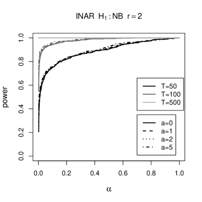
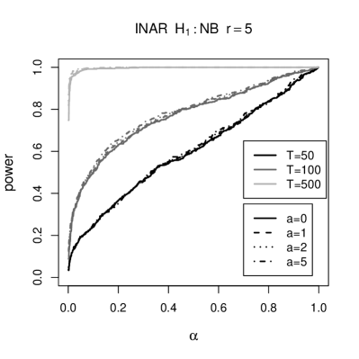
Figure 1: Power of the test for a Poisson INAR(1) against an INAR(1) model with Negative Binomial innovations with dispersion parameter $r$.

Under alternative (b), the innovations are generated from a mixture of two Poisson distributions (always with mixture mean equal to 4) of the form $\phi\mathsf{Po}(\lambda_{1})+(1-\phi)\mathsf{Po}(\lambda_{2})$, where $\mathsf{Po}(\lambda)$ denotes the Poisson distribution with mean $\lambda$. The estimated power for $\lambda_{1}=6$ and $\phi=0.3$ or $\phi=0.5$ is plotted in Figure 2. We can see that $\phi=0.5$ leads to noticeably larger power compared to $\phi=0.3$. Likewise for a larger $\lambda_{1}$ one would obtain a larger power (results not shown). On the other hand, if $|\theta-\lambda_{1}|$ decreases then the mixture distribution gets closer to the Poisson distribution and consequently a relatively long series is needed in order to obtain a reasonable power.

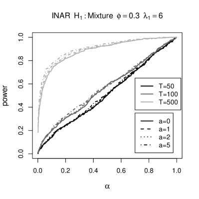
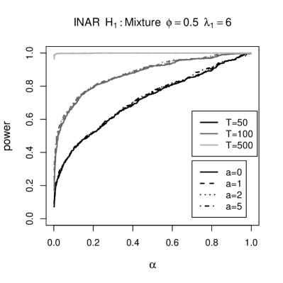
Figure 2: Power of the test for a Poisson INAR(1) under an INAR(1) with innovations following a mixture of two Poisson distributions with mixing parameter $\phi$.

The alternative (c) is plotted in Figure 3. Here, the innovations are assumed to follow a mixture $\phi\mathsf{D}_{0}+(1-\phi)\mathsf{Po}(\lambda)$, where $\mathsf{D}_{0}$ denotes the Dirac measure at $0$. As expected, the power increases with the value of $\phi$.

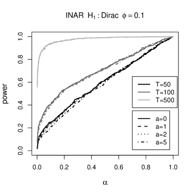
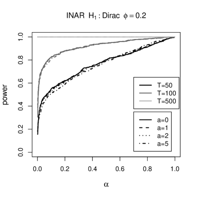
Figure 3: Power of the test for a Poisson INAR(1) under an INAR(1) with innovations following a mixture of a Poisson distribution, and a Dirac measure at 0 with weight $\phi$.

Finally, Figure 4 (left panel) shows that the test is also able to distinguish between a Poisson INAR(1) model and data generated from a different model, namely a Poisson INARCH(1) model, provided that the series is long enough. The opposite situation, discussed later, is plotted in the right panel.

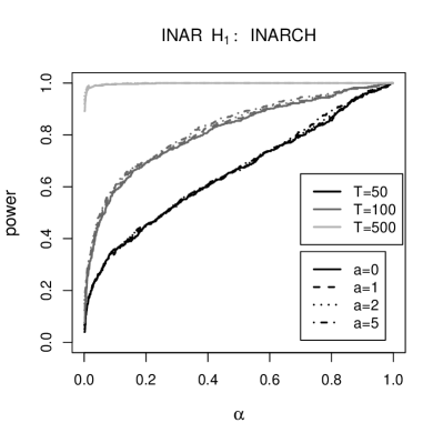
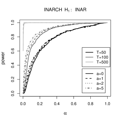
Figure 4: Power of the test for a Poisson INAR(1) under a Poisson INARCH(1) (left panel). Power for a Poisson INARCH(1) under a Poisson INAR(1) (right panel).

To sum up, the presented results show that the power of the test is satisfactory provided that the alternative is far enough from the null hypothesis, or the sample size is large. Moreover, the simulations reveal some differences in powers of the test for different values of the weight parameter  $a$. However, it seems that it is not possible to generally recommend one particular value of $a$. For instance, for the case (c) (innovations following a mixture of a Dirac measure at 0 and Poisson distribution), it seems that $a=0$ performs the best. On the other hand, one can observe the opposite or no effect of $a$ in the remaining settings.

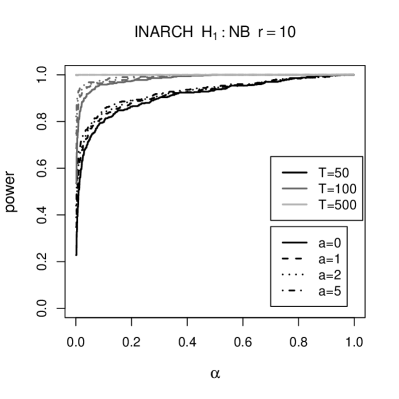
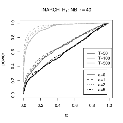
Figure 5: Power of the test for a Poisson INARCH(1) under a Negative Binomial INARCH(1) with dispersion parameter $r=10$ and $r=40$.

The power of the test for the null hypothesis of a Poisson INARCH(1) was studied under the following alternatives: (a) a Negative Binomial INARCH(1), (b) a Poisson INAR(1), (c) a Poisson INGARCH(1,1), and (d) a Poisson INARCH(1) with a level change.

Altervative (a) corresponds to the model (4) with $G$ being the Negative Binomial distribution with a dispersion parameter $r$, see [24]. Results for dispersion parameter $r=10$ and $r=40$ are plotted in Figure 5. Similarly to INAR(1) with Negative Binomial innovations, the power of the test decreases with increasing $r$, and in this case, larger values of $a$ seem to lead slightly larger power compared to $a=0$.

Alternative (b) corresponds to a Poisson INAR(1), and it is presented in Figure 4, right panel. In this case, it seems that larger values of $a$ might yield noticeable larger power compared to $a=0$. Moreover, the effect of $a$ is more substantial here compared to the situation in the left panel, i.e. testing of INAR(1) under INARCH(1) alternative.

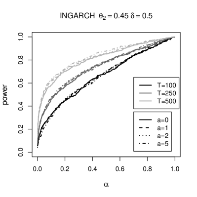
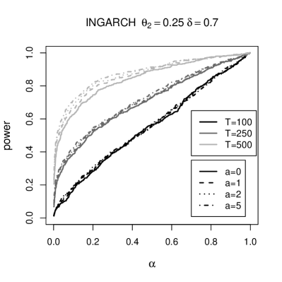
Figure 6: Power of the test for a Poisson INARCH(1) under a Poisson INGARCH(1,1) alternative with parameters $\theta_{2}$ and $\delta$.

Figure 7: Power of the test for a Poisson INARCH(1) under a Poisson INARCH(1) with level shift with parameters $\delta=4$ or $\delta=8$, and $\phi=0.1$ or $\phi=0.3$.

In alternative (c), the data are generated from a Poisson INGARCH(1,1) model of the form

$$Y_{t}|\mathcal{I}_{t}\sim\mathsf{Po}(\lambda_{t}),\ \lambda_{t}=\theta_{1}+\theta_{2}Y_{t-1}+\delta\lambda_{t-1},$$

see e.g. [27]. Figure 6 shows results for $\theta_{1}=0.1$ and $(\theta_{2},\delta)=(0.45,0.5)$ and $(\theta_{2},\delta)=(0.25,0.70)$. The unconditional mean of $Y_{t}$ is equal to $2$ in both settings. Clearly, the power growths with an increasing sample size $T$. When comparing different values of $a$, it seems that for larger sample sizes ($T=500$) larger values of $a$ lead to a larger power compared to $a=0$. However, for smaller sample sizes ($T=100$) one might observe the opposite. Furthermore, when keeping $\theta_{1}$ and the unconditional mean fixed (i.e. keeping $\theta_{2}+\delta$ fixed), the power does not always grow with increasing $\delta$ for a fixed sample size $T$. Specifically, we do observe this behavior for $T=500$, but opposite results are obtained for $T=100$ and $T=250$.

Finally, alternative (d) considers a Poisson INARCH(1) model with a level shift, i.e. a model of the form

$$Y_{t}|\mathcal{I}_{t-1}\sim\mathsf{Po}(\lambda_{t}),\ \lambda_{t}=\theta_{1}+\theta_{2}Y_{t-1}+\delta I[t\geq\tau_{0}],$$

where $\tau_{0}$ is a specific time moment, and $I[\cdot]$ is an indicator function. This model is a special case of a Poisson INARCH(1) with an intervention in [25]. Various choices for the parameters $\theta_{1},\theta_{2}$, and $\delta$ where considered, together with $\tau_{0}=\phi\cdot T$, with $\phi\in(0,1)$. Results for $(\theta_{1},\theta_{2})=(4,0.60)$ and $\delta=4$ and $\delta=8$ are presented in Figure 7. For simplicity, we restrict to $a=1$, $T=50$ and $100$ and $\phi=0.1$ and $\phi=0.3$. As expected, the power of the test growths substantially with the size of the shift $\delta$. For a fixed value of $\phi$, the power also slowly increases with an increasing sample size $T$. Furthermore, the simulations indicate that different values of $a$ seem to lead to comparable powers and no general recommendation about “the most appropriate” value for $a$ can be given here (results not shown).

7.2 INAR(2)

In order to illustrate the behavior of the bootstrap test for higher order models, we present a short simulation study for a Poisson INAR(2) model with $p_{1}=0.3$, $p_{2}=0.2$ and $\theta=\mathbb{E}\varepsilon_{t}=5$. Under the alternatives, we consider INAR(2) models with innovations $\varepsilon_{t}$ following (a) the Negative Binomial distribution with dispersion parameter $r$ and (b) a mixture of Poisson and Dirac measure at 0 with weights $1-\phi$ and $\phi$, respectively. For the sake of brevity only results for $a=0$ are shown.

Table 7.2 indicates that under the null hypothesis, the test generally keeps the prescribed significance level $\alpha$. The power of the test under the alternatives is plotted in Figure 8. The results are in correspondence with those of INAR(1). In particular, under the alternative (a) the power decreases with increasing dispersion parameter $r$. Under the alternative (b), the power increases with the value of $\phi$. In both cases, the power growths with an increasing sample size $T$. For $T=500$ we get very high power for all the considered settings — in particular, the power is always greater than 90% for $\alpha=0.05$.

Size of the test for the Poisson INAR(2) model. $\alpha$ $T$ 0.01 0.05 0.1 50 0.006 0.038 0.096 100 0.010 0.040 0.076 250 0.010 0.044 0.106 500 0.006 0.050 0.094

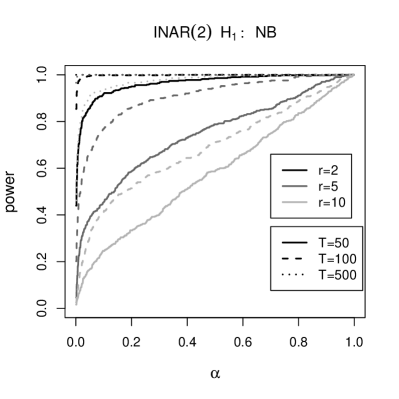
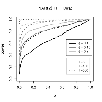
Figure 8: Power of the test for a Poisson INAR(2) model under an INAR(2) with innovations following (a) the Negative Binomial distribution with dispersion parameter $r$ (left panel) and (b) the mixture of Poisson and Dirac measure at 0 with weight $\phi$ (right panel).

8 Application

We illustrate the goodness-of-fit test on five time series previously analyzed in [33]. The data consist of monthly number of claims of short-term disability benefits made by injured workers to the British Columbia Workers Compensation Board (WCB). The recorded period is January 1985 to December 1994. The five series correspond to five different injury categories: burn injuries, soft tissue injuries, cuts, dermatitis and dislocations. The first series of burn injuries is corrected by excluding one long duration claimant according to [33, p. 159].

Freeland [33] considered an INAR(1) model for the five series. Except series 3 (cuts) the classical stationary INAR(1) with Poisson marginals was chosen for the analysis. For series 3, an INAR(1) model with Poisson marginals and seasonality modelled by trigonometric functions was fitted. This series was further investigated e.g. by Zhu and Joe [34], who improved the previous model by considering also Negative Binomial marginals.

We applied the suggested goodness–of–fit test in order to test the appropriateness of the stationary Poisson INAR(1) for the five series. The test statistic $S_{T}$ was computed using the weight function $w(u)=u^{a}$ for $a=0,1,2,5,10$. The corresponding p-value was computed from 999 bootstrap samples.

p–value of the goodness of fit test for the five claim series for $a=0,1,2,5,10$. $a$ series 0 1 2 5 10 1 0.653 0.652 0.698 0.771 0.862 2 0.561 0.596 0.579 0.662 0.665 3 0.020 0.002 0.001 0.000 0.000 4 0.270 0.270 0.295 0.386 0.506 5 0.444 0.486 0.579 0.661 0.749

The obtained results are summarized in Table 8. We can observe that our results corroborate the results of [33]. Specifically, for series 1,2,4, and 5 the null hypothesis that the series follows a Poisson INAR(1) model is not rejected. On the other hand, for series 3 we get significant p-values, which indicate that a simple stationary Poisson INAR(1) model is not appropriate here.

Acknowledgements

We thank to both anonymous referees for careful reading and a number of valuable comments which led to improvement the presentation of the results. The research of Simos Meintanis was partially supported by grant number 11699 of the Special Account for Research Grants (ELKE) of the National and Kapodistrian University of Athens. The research of Marie Hušková was partially supported by grant GAČR P201/12/1277. The research of Šárka Hudecová was partially supported by the Czech Science Foundation project “DYME – Dynamic Models in Economics” No. P402/12/G097.

9 Proofs

Proof of Theorem 4.1. Recall that we assume that $\{Y_{t}\}_{t\in\mathbb{N}}$ is a sequence of stationary and ergodic variables. Hence, the sequence $\{h(Y_{t})\}_{t\in\mathbb{N}}$ is stationary and ergodic for any measurable function $h$ such that $\mathbb{E}|h(Y_{1})|<\infty$. In particular, this holds for $h(y)=u^{y}-(1+p(u-1)^{y})$ for all $u\in[0,1]$.

In the following we drop the index $0$ in $p_{0}$ and $\theta_{0}$ whenever it is not confusing, and $D$ denotes generic constants.

First of all notice that the test statistic $S_{T}$ in eqn. (5) has asymptotically the same distribution as

$${\cal{S}}_{T}=\int_{0}^{1}\left(\frac{1}{\sqrt{T}}\sum_{t=2}^{T}\widehat{Z}_{t}(u)\right)^{2}w(u)du,$$ (29)

where $\widehat{Z}_{t}(u)=Z_{t}(u;\widehat{p}_{T},\widehat{\theta}_{T})$ with $Z_{t}$ defined in (16). Let us study the process ^Z_T (u)= 1T∑_t=2^T ^Z_t(u) = 1T∑_t=2^T( u^Y_t-(1+^p_T(u-1))^Y_t-1 g_0,ε (u;^θ_T))

for a fixed $u\in[0,1]$. Applying the Taylor expansion we get the decomposition: ^Z_T (u)= J_0T(u)+J_1T(u)+ J_2T(u)+R_T(u), where $R_{T}(u)$ is a remainder term (it does not influence the limit behavior) and

$$J_{0T}(u)= \ \frac{1}{\sqrt{T}}\sum_{t=2}^{T}\Big{(}u^{Y_{t}}-(1+p(u-1))^{Y_{t-1}}g_{\varepsilon}(u;\theta)\Big{)},$$

$$J_{1T}(u)= -\sqrt{T}(\widehat{p}_{T}-p)\frac{1}{T}\sum_{t=2}^{T}\Big{(}(1+p(u-1))^{Y_{t-1}-1}Y_{t-1}(u-1)\Big{)}g_{\varepsilon}(u;\theta),$$

$$J_{2T}(u)= -\sqrt{T}(\widehat{\theta}_{T}-\theta)\frac{1}{T}\sum_{t=2}^{T}(1+p(u-1))^{Y_{t-1}}\Big{(}\frac{\partial g_{\varepsilon}(u;\theta)}{\partial\theta}\Big{)}.$$

Standard arguments give that

$$|R_{T}(u)|\leq D\Big{(}T(\widehat{p}_{T}-p)^{2}+T(\widehat{\theta}_{T}-\theta)^{2}\Big{)}\Big{(}\frac{1}{T^{3/2}}\sum_{t=2}^{T}Y_{t-1}^{2}+\frac{1}{\sqrt{T}}\Big{)}(1+v(u))$$

uniformly for $u\in[0,1]$ for some $D>0$. This together with assumptions (A.3) – (A.4) immediately implies

$$\int_{0}^{1}R^{2}_{T}(u)w(u)du=o_{P}(1).$$

Next we study $J_{1T}(u)$ and $J_{2T}(u)$. In view of the ergodicity of $\{Y_{t}\}_{t\in\mathbb{N}}$ and smoothness of $J_{1T}(u)$ and $J_{2T}(u)$ in $u\in[0,1]$ we observe that as $T\to\infty$

$$\frac{1}{T}\sum_{t=2}^{T}\Big{(}(1+p(u-1))^{Y_{t-1}-1}Y_{t-1}(u-1)\Big{)}g_{\varepsilon}(u;\theta) \to h_{1}(p,\theta;u),\,a.s.,$$

$$\frac{1}{T}\sum_{t=2}^{T}\Big{(}(1+p(u-1))^{Y_{t-1}}\Big{)}\frac{\partial g_{\varepsilon}(u;\theta)}{\partial\theta} \to h_{2}(p,\theta;u),\,a.s.$$

for $u\in[0,1]$, where

$$h_{1}(p,\theta;u)= \frac{\partial g_{Y}(1+p(u-1))}{\partial p}(u-1)g_{\varepsilon}(u;\theta)$$

$$h_{2}(p,\theta;u)= \mathbb{E}\Big{(}(1+p(u-1))^{Y_{t-1}}\Big{)}\frac{\partial g_{\varepsilon}(u;\theta)}{\partial\theta}=g_{Y}(1+p(u-1))\frac{\partial g_{\varepsilon}(u,\theta))}{\partial\theta}.$$

Since —((1+ p(u-1))^Y_t-1-1 Y_t-1 (u-1)) g_ε (u;θ)—≤Y_t, u∈[0,1], and —((1+p(u-1))^Y_t-1) ∂gε(u;θ)∂θ—≤—∂gε(u;θ)∂θ—, u∈[0,1] and since the random variables on the r.h.s. have finite second moments, the uniform ergodicity theorem, see [35, Theorem 6.2], can be applied and it further implies that

$$\int_{0}^{1}\Big{(}J_{1T}(u)-J_{1T0}(u)\Big{)}^{2}w(u)du+\int_{0}^{1}\Big{(}J_{2T}(u)-J_{2T0}(u)\Big{)}^{2}w(u)du=o_{P}(1),$$

where

$$J_{1T0}(u) =-\frac{1}{\sqrt{T}}\sum_{t=2}^{T}\ell_{1}({\bf{Y}}_{t-q};p,\theta)h_{1}(p,\theta;u),$$

$$J_{2T0}(u) =-\frac{1}{\sqrt{T}}\sum_{t=2}^{T}\ell_{2}({\bf{Y}}_{t-q};p,\theta)h_{2}(p,\theta;u).$$

Hence, it remains to study the asymptotic behavior of Q_1T= ∫_0^1 ( J_0T(u)+ J_1T0(u)+J_2T0(u))^2 w(u)du.

In order to obtain the limiting distribution of $\cal{S}_{T}$ in (29) we apply Theorem 22 in [36, p. 380-381]. We need to verify its assumptions. Particularly, we need to show that

1. $\sup_{T}\mathbb{E}Q_{1T}<\infty,$

2. $\mathbb{E}|J^{2}_{0T}(u)-J^{2}_{0T}(s)|+\mathbb{E}|J^{2}_{1T0}(u)-J^{2}_{1T0}(s)|+\mathbb{E}|J^{2}_{2T0}(u)-J^{2}_{2T0}(s)|\leq D|u-s|^{\kappa},\,$ for some $\kappa>0$ and all $u,s\in[0,1],$

3. for any real numbers $a_{vj},\,u_{v}\in[0,1],\,v=1,\ldots,k,\,j=0,1,2$ the asymptotic distribution of $\sum_{v=1}^{k}(a_{0v}J_{0T}(u_{v})+a_{1v}J_{1T0}(u_{v})+a_{2v}J_{2T0}(u_{v}))$ is normal with zero mean.

To check validity of (I.) we notice that $J_{0T}(u)+J_{1T0}(u)+J_{2T0}(u)$ are sums of martingale differences for any fixed $u$. Thus, direct calculations give

$$\mathbb{E} (J_{0T}(u)+J_{1T0}(u)+J_{2T0}(u))^{2}=\frac{T-1}{T}\mathbb{E}\Big{(}u^{Y_{t}}-(1+p(u-1))^{Y_{t-1}}g_{\varepsilon}(u;\theta)$$

$$-\ell_{1}({\bf{Y}}_{t-q};p,\theta)h_{1}(p,\theta;u)-\ell_{2}({\bf{Y}}_{t-q};p,\theta)h_{2}(p,\theta;u)\Big{)}^{2}$$

$$\leq D\Big{(}g^{2}_{\varepsilon}(u;\theta)+h^{2}_{1}(p,\theta;u)\mathbb{E}\ell^{2}_{1}({\bf Y}_{t-q};p,\theta)+h^{2}_{2}(p,\theta;u)\mathbb{E}\ell^{2}_{2}({\bf Y}_{t-q};p,\theta)+1\Big{)}.$$

This easily implies (I.). In addition, a central limit theorem for sums of martingale differences can be applied here and this immediately gives (III.).

Concerning (II.) notice that

$$\mathbb{E}|J^{2}_{0T}(u_{1})-J^{2}_{0T}(u_{2})| \leq\Big{(}\mathbb{E}(J_{0T}(u_{1})-J_{0T}(u_{2}))^{2}\mathbb{E}(J_{0T}(u_{1})+J_{0T}(u_{2}))^{2}\Big{)}^{1/2}$$

$$\leq D\Big{(}\mathbb{E}(J_{0T}(u_{1})-J_{0T}(u_{2}))^{2}\Big{)}^{1/2},$$

where we used the Cauchy-Schwarz inequality and (I.). Since $J_{0T}(u_{1})-J_{0T}(u_{2})$ is the sum of a martingale differences sequence we also get that

$$\mathbb{E}(J_{0T}(u_{1})-J_{0T}(u_{2}))^{2}=\frac{T-1}{T}\mathbb{E}(u_{1}^{Y_{t}}-u_{2}^{Y_{t}}$$

$$-\big{(}(1+p(u_{1}-1))^{Y_{t-1}}-(1+p(u_{2}-1))^{Y_{t-1}}\big{)}g_{\varepsilon}(u_{1};\theta)$$

$$-(1+p(u_{2}-1))^{Y_{t-1}}(g_{\varepsilon}(u_{1};\theta)-g_{\varepsilon}(u_{2};\theta))\Big{)}^{2}$$

$$\leq D(|u_{1}-u_{2}|^{2}\mathbb{E}Y_{t}^{2}+|g_{\varepsilon}(u_{1};\theta)-g_{\varepsilon}(u_{2};\theta)|)\leq D|u_{1}-u_{2}|,$$

where we used the following simple inequalities:

$$|u_{1}^{Y_{t}}-u_{2}^{Y_{t}}|\leq|u_{1}-u_{2}|Y_{t}(u_{1}^{Y_{t}-1}+u_{1}^{Y_{t}-1})\leq 2|u_{1}-u_{2}|Y_{t},$$

$$|(1+p(u_{1}-1))^{Y_{t-1}}-(1+p(u_{2}-1))^{Y_{t-1}}|\leq D|u_{1}-u_{2}|Y_{t-1}$$

$$|g_{\varepsilon}(u_{1},\theta)-g_{\varepsilon}(u_{2},\theta)|\leq D|u_{1}-u_{2}|$$

for some $D>0$. The last inequality follows from the assumption (A.1).

Concerning $J_{jT0}(u_{1})-J_{jT0}(u_{2}),j=1,2,$ we see that E—J_jT0(u_1)- J_jT0(u_2)—^2≤D Eℓ^2_j(Y_t-q;p, θ) —h_j(p,θ;u_1)-h_j(p,θ;u_2)—^2,   j=1,2. By assumptions $\mathbb{E}\ell^{2}_{j}({\bf Y}_{t-q};p,\theta)$ is finite and does not depend on $u_{1},u_{2}$. Hence, we just need that

$$|h_{j}(p,\theta;u_{1})-h_{j}(p,\theta;u_{2})|^{2}\leq D|u_{1}-u_{2}|^{\kappa_{0}},\quad j=1,2,$$

for some $\kappa_{0}>0$ which holds true by the assumptions. ∎

Proof of Theorem 4.4. The proof follows the same lines as Theorem 4.1. Clearly,

$$\exp \{(\widehat{\theta}_{1T}+\widehat{\theta}_{2T}Y_{t-1})(u-1)\}=\exp\{(\theta_{1}+\theta_{2}Y_{t-1})(u-1)\}$$

$$\times\Big{(}1+((\widehat{\theta}_{1T}-\theta_{1})+(\widehat{\theta}_{2T}-\theta_{2})Y_{t-1})(u-1)\Big{)}+R_{T}(u),$$

$$|R_{t,T}(u)| \leq\exp\{(\theta_{1}+\theta_{2}Y_{t-1})(u-1)\}\Big{(}(\widehat{\theta}_{1T}-\theta_{1})^{2}+(\widehat{\theta}_{2T}-\theta_{2})^{2}Y^{2}_{t-1}\Big{)}.$$

By the assumptions

$$\int_{0}^{1}\frac{1}{T}\large(\sum_{t=2}^{T}R_{t,T}(u)\large)^{2}w(u)du =O_{P}\Big{(}\frac{1}{T}\int_{0}^{1}\mathbb{E}\exp\{2(\theta_{1}+\theta_{2}Y_{t-1})(u-1)\}(1+Y_{t-1}^{4})w(u)du\Big{)}$$

$$=O_{P}(T^{-1}).$$

After a few steps similar to the steps in INAR(1) we get that under the considered assumptions and under the null hypothesis, $S_{T}$ has the same limit distribution as

$$\int_{0}^{1} \frac{1}{T}\Big{(}\sum_{i=2}^{T}\Big{(}u^{Y_{t}}-\exp\{(\theta_{1}+\theta_{2}Y_{t-1})(u-1)\}(u-1)$$

$$+ \ell_{1}({\bf Y}_{t-q};\theta_{1},\theta_{2})r_{1}(u;\theta_{1},\theta_{2})$$

$$+ \ell_{2}({\bf Y}_{t-q};\theta_{1},\theta_{2})r_{2}(u;\theta_{1},\theta_{2})\Big{)}^{2}w(u)du.$$

Hence, the assumptions of Theorem 22 in [36] are fulfilled and our theorem is proved. ∎

References

• [1] Koul H., Mimoto N. and Surgailis D. Goodness–of–fit tests for long memory moving average marginal density. Metrika. 2013; 76: 205–224.
• [2] Koul H. and Mimoto N. A goodness–of–fit test for GARCH innovation density. Metrika 2012; 75: 127–149.
• [3] Koul H. and Surgailis D. Goodness–of–fit testing under long memory. J Statist Plann Inference. 2010; 140: 3742–3753.
• [4] Horváth L. and Zitikis R. Testing goodness–of–fit based on densities of GARCH innovations. Econometric Theory. 2006; 22: 457–482.
• [5] Horváth L., Kokoszka P. and Teyssiére G. Bootstrap misspecification tests for ARCH based on the empirical process of squared residuals. J Statist Comput Simul. 2004; 74: 469–485.
• [6] Epps T.W. Testing that a stationary time series is Gaussian. Ann Statist. 1987; 15: 1683–1698.
• [7] Cuesta–Albertos J.A., Gamboa F. and Nieto–Reyes A. A random projection based test of Gaussianity for stationary processes. Comput Statist Data Anal. Forthcoming 2013.
• [8] Ghosh S. Normality testing for a long-memory sequence using the J Statist Plann Inference. 2013; 143: 944–954.
• [9] Klar B., Lindner F. and Meintanis S.G. Specification tests for the error distribution in GARCH models. Comput Statist Data Anal. . 2012; 56: 3587–3598.
• [10] Fokianos K. and Neumann M.H. A goodness–of–fit test for Poisson count processes. Electron J Stat. 2013; 7: 793–819.
• [11] Rothe C. and Wied D. Misspecification testing in a class of conditional models J Amer Statist Assoc. 2013; 108: 314–324.
• [12] McKenzie E. Some simple models for discrete variate time series. Water Resour Bull. 1985; 21: 645–650.
• [13] Al–Osh M.A. and Alzaid A.A. (1987). First–order integer–valued autoregressive (INAR(1)) process. J Time Series Anal. 1987; 8: 261–275.
• [14] Alzaid A.A. and Al–Osh M.A. First–order integer–valued autoregressive (INAR(1)) process: Distributional and regression properties. Stat Neerl. 1988; 42: 53–61.
• [15] Alzaid A.A. and Al–Osh M.A. An integer–valued $p$th–order autoregressive structure (INAR($p$)) process. J Appl Probab. 1990; 27: 314–324.
• [16] Du J.G. and Li Y. The integer-valued autoregressive (INAR($p$)) model. J Time Series Anal. 1991; 12: 129–142.
• [17] McKenzie E. Discrete variate time series. In Shanbhag and Rao (eds.): Handbook of Statistics, 2003; 21: 573–606.
• [18] Wei$\upbeta$ C.H. Thinning operations for modeling time series of counts–a survey. Adv Stat Anal., 2008; 92: 319–341.
• [19] Pavlopoulos H. and Karlis D. . INAR(1) modeling of overdispersed count series with an enviromental application. Environmetrics. 2008; 19: 369–393.
• [20] Barczy M., Ispány M., Pap G., Scotto M. and Silva M.A. Innovation outliers in INAR(1) models. Comm Statist Theory Methods. 2010; 39: 3343–3362.
• [21] Fokianos K., Rahbek A. and Tjostheim D. Poisson autoregression. J Amer Statist Assoc. 2009; 104: 1430–1439.
• [22] Fokianos K. and Tjostheim D. Nonlinear Poisson autoregression. Ann Inst Stat Math. 2012; 64: 1205–1225.
• [23] Fokianos K. Some progress in count time series models. Statistics. 2011; 45: 49–58.
• [24] Zhu F. A negative binomial integer–valued GARCH model. J Time Series Anal. 2011; 32: 54–67.
• [25] Fokianos K. and Fried R. Interventions in INGARCH processes. J Time Series Anal. 2010; 31: 210–225.
• [26] Meintanis, S.G. and Karlis, D. Validation tests for the innovation distribution in INAR time series models. Comput Statist. 2014; DOI 10.1007/s00180-014-0488-z.
• [27] Ferland R., Latour A. and Oraichi D. Integervalued GARCH processes. J Time Series Anal. 2006; 27: 923–942.
• [28] Neumann, M. H. Absolute regularity and ergodicity of Poisson count processes. Bernoulli. 2011; 17: 1268–1284.
• [29] Klimko L.A. and Nelson P.I. On conditional least squares estimation for stochastic processes. Ann Statist. 1987; 6: 629–642.
• [30] Genest C. and Rémillard B. Validity of the parametric bootstrap for goodness–of–fit testing in semiparametric models. Ann Inst Henri Poincaré Probab Stat. 2008; 44: 1096–1127.
• [31] Leucht A. and Neumann M.H. Degenerate $U$– and $V$–statistics under ergodicity: asymptotics, bootstrap and applications in statistics. Ann Inst Statist Math. 2013 65: 349–386.
• [32] R Development Core Team. R: A Language and Environment for Statistical Computing. R Foundation for Statistical Computing, Vienna, Austria; 2013.
• [33] Freeland R.K. Statistical Analysis of Discrete Time series with Application to the Analysis of Workers’ Compensation Claims Data [PhD thesis]. Management Science Division, Faculty of Commerce and Business Administration, University of British Columbia; 1998.
• [34] Zhu F. and Joe H. Modelling count data time series with Markov processes based on binomial thinning. J Time Series Anal. 2006; 27: 725–738.
• [35] Rao R. Relations between weak and uniform convergence of measures with applications. Ann Math Statist. 1962; 33: 659–680.
• [36] Ibragimov I. and Hasminskii R. Statistical Estimation; Asymptotic Theory. Springer Verlag, New York; 1981.
\appendices