Instability of Magnetized Ionization Fronts Surrounding H II Regions

Abstract

An ionization front (IF) surrounding an H II region is a sharp interface where a cold neutral gas makes transition to a warm ionized phase by absorbing UV photons from central stars. We investigate the instability of a plane-parallel D-type IF threaded by parallel magnetic fields, by neglecting the effects of recombination within the ionized gas. We find that weak D-type IFs always have the post-IF magnetosonic Mach number $\mathcal{M}_{\rm M2}\leq 1$. For such fronts, magnetic fields increase the maximum propagation speed of the IFs, while reducing the expansion factor $\alpha$ by a factor of $1+1/(2\beta_{1})$ compared to the unmagnetized case, with $\beta_{1}$ denoting the plasma beta in the pre-IF region. IFs become unstable to distortional perturbations due to gas expansion across the fronts, exactly analogous to the Darrieus-Landau instability of ablation fronts in terrestrial flames. The growth rate of the IF instability is proportional linearly to the perturbation wavenumber as well as the upstream flow speed, and approximately to $\alpha^{1/2}$. The IF instability is stabilized by gas compressibility and becomes completely quenched when the front is D-critical. The instability is also stabilized by magnetic pressure when the perturbations propagate in the direction perpendicular to the fields. When the perturbations propagate in the direction parallel to the fields, on the other hand, it is magnetic tension that reduces the growth rate, completely suppressing the instability when $\mathcal{M}_{\rm M2}^{2}<2/(\beta_{1}-1)$. When the front experiences an acceleration, the IF instability cooperates with the Rayleigh-Taylor instability to make the front more unstable.

1 Introduction

H II regions are volumes of ionized gas formed by absorbing UV photons emitted by newborn massive stars. Since the ionized gas is overpressurized by about two orders of magnitude compared to the surrounding neutral medium, it naturally expands to affect the structure and dynamics of a surrounding interstellar medium (ISM). Photoionization appears to play a dual role in regulating star formation in the ISM. On one hand, it can evaporate and disrupt parental molecular clouds, limiting the efficiency of star formation to about a few percents (Matzner, 2002; Krumholz et al., 2006; Walch et al., 2012; Dale et al., 2012). On the other hand, the expansion of H II regions may sustain turbulence in clouds (Mellema et al., 2006; Krumholz et al., 2006; Gritschneder et al., 2010; Dale et al., 2012), and trigger gravitational collapse of compressed shells (Elmegreen & Lada, 1977; Hosokawa & Inutsuka, 2006; Dale et al., 2009; Iwasaki et al., 2011) as well as pre-existing clumps in the surrounding medium (e.g., Sandford et al., 1982; Bertoldi, 1989; Bisbas et al., 2011), tending to promote further star formation. Understanding how H II regions evolve may thus be the first step to understand the effect of the star formation feedback on the ISM (see Krumholz et al. 2014, for a recent review).

A number of pioneering studies have explored the dynamical expansion of an H II region (Strömgren 1939; Kahn 1954; Goldsworthy 1958; Axford 1961; Mathews 1965; see also Yorke 1986; Shu 1992). Soon after a central ionizing source is turned on, an ionization front (IF) develops to separate a warm ionized gas with temperature $T\sim 10^{4}\;{\rm K}$ from a cold neutral gas with $T\sim 10^{2}\;{\rm K}$, with thickness of order of only a few photon mean free paths. At early times, the ionizing photon flux is very large and the IF advances into the neutral medium supersonically, without inducing gas motions. In this early phase, the IF is termed “weak R-type” (Kahn, 1954). After roughly a few recombination times (typically $\sim 10^{3}$ yrs), the initial Strömgren sphere is established within which the recombination rate balances the ionizing rate. At this point, the IF stops propagating and turns to a “R-critical” front. Since the ionized gas behind the IF moves at the sonic speed with respect to the IF, it is able to launch shock waves into the regions ahead of the IF, which in turn makes the R-critical front switch to a “D-critical” front. After this transition, the expansion of the IF is driven by the pressure difference between the ionized and neutral gas. The IF becomes “weak D-type” and moves subsonically with respect to the neutral gas. Given that the main-sequence lifetime of O/B stars is typically $\sim 10^{6}-10^{7}$ yrs, H II regions spend most of their lives in the weak D-type phase.

While the early efforts based on one-dimensional models under spherical symmetry provide valuable insights on the overall evolution, H II regions are abound with various substructures such as globules, filaments, gaseous pillars (or “elephant trunks”), etc. that cannot be explained by the one-dimensional models (e.g., Sugitani et al. 1991; Hester et al. 1996; Churchwell et al. 2006). One promising explanation may be that these non-spherical structures result from pre-existing density inhomogeneities and/or turbulent motions in the background medium. Numerical simulations indeed showed that ionizing radiation illuminating on a turbulent, inhomogeneous medium forms non-axisymmetric structures, elongated away from the ionizing source, which may undergo gravitational collapse (e.g., Gritschneder et al. 2010; Arthur et al. 2011; Tremblin et al. 2012a, b).

Although less well-recognized, instability of IFs can be another route to the formation of non-spherical structures. Frieman (1954) and Spitzer (1954) suggested that IFs are susceptible to the Rayleigh-Taylor instability (RTI) when the front is accelerating away from the central source, which may occur due to a steep gradient of the background density or time-varying radiation intensity. Vandervoort (1962) performed a linear stability analysis of an unmagnetized, planar weak D-type IF by including a steady motion of gas relative to the front. He found that such steady-state IFs even without acceleration are unstable at all wavelengths, with the growth rate inversely proportional to the perturbation wavelength. Axford (1964) subsequently showed that the long-wavelength modes are stabilized by the attenuation of radiation due to hydrogen recombination in the perturbed ionized gas if the radiation is normal to the front. Allowing for finite temperature ratio between the neutral and ionized phases, Saaf (1966) obtained an approximate, closed-form expression for the growth rate of the IF instability. Later, Sysoev (1997) discovered the existence of long-wavelength unstable modes even in the presence of recombination. Williams (2002) further extended the previous studies by including oblique incident angles of the ionizing radiation relative to the front, and carried out local isothermal simulations of the instability to study its nonlinear development. By running simulations of expanding H II regions, Garcia-Segura & Franco (1996) and Whalen & Norman (2008) suggested that a shocked shell undergoes a thin-shell instability (Vishniac, 1983) to grow into sword-like structures. Ricotti (2014) performed a stability analysis of accelerating IFs in the limit of incompressible fluids and showed that the recombination stabilizes RTI of IFs (see also Mizuta et al. 2005; Park et al. 2014).

Despite these efforts on the IF instability, however, there are still two main issues that remain to be answered. First, what is the physical nature of the instability? Vandervoort (1962) argued that the IF instability results from a mechanism similar to the “rocket effect” of gradually evaporating clouds (Kahn, 1954; Oort & Spitzer, 1955). However, the rocket effect acting on the IF can always make the IF move away from the central source and is thus unable to explain the wavy movement of the perturbed IF toward the source, which is the key in the operation of the IF instability, as we will show below. The second issue concerns the effect of magnetic fields on the IF instability. Observations indicate that the ISM around H II regions are permeated by magnetic fields. The typical values for the ratio of magnetic to thermal pressure are $\sim 0.3$ and $\sim 0.04$ in cold neutral and molecular clouds, respectively (Crutcher, 1999; Heiles & Crutcher, 2005). The line-of-sight component of magnetic fields inside five Galactic H II regions based on Faraday rotation diagnostics is estimated to be in the range of $B_{\rm los}\sim 2$–$6\,\mu{\rm G}$, corresponding to subthermal magnetic pressure (Harvey-Smith et al. 2011; see also Heiles & Chu 1980; Heiles et al. 1981; Rodríguez et al. 2012). On the other hand, Zeeman observations of H I and OH absorption lines reveal that the interfaces between the ionized and molecular gases are strongly magnetized with $B_{\rm los}\sim 50$–$300\,\mu{\rm G}$ and $\sim 250$–$750\,\mu{\rm G}$ for Orion’s Bar and M17, respectively (Brogan et al., 1999; Brogan & Troland, 2001; Brogan et al., 2005). Using hydrostatic models, Pellegrini et al. (2007, 2009) confirmed that these clouds are indeed dominated by magnetic pressure.

Importance of magnetic fields associated with IFs has been emphasized by several authors. For instance, Lasker (1966) showed that D-type IFs may contain strong magnetic fields when preceded by an isothermal shock. Redman et al. (1998) calculated the jump conditions for IFs with magnetic fields parallel to the fronts. Williams et al. (2000) show that an IF with oblique magnetic fields drives fast- and slow-mode shocks separately as it slows down, suggesting IFs should be subclassified according to the propagation speed. Numerical simulations showed that H II regions threaded by uniform magnetic fields expand aspherically and that both shock strength and density contrast across the IF are reduced in regions where the magnetic fields are parallel to the front (Krumholz et al., 2007; Mackey & Lim, 2011). Although these simulations also reported the deformation of IFs during nonlinear evolution, they lacked spatial resolution to capture the instability of IFs.

In this paper we address the two issues mentioned above by performing a linear stability analysis of weak D-type IFs with and without magnetic fields. We also include the acceleration/deceleration term in the momentum equation in order to study the combined effects of the RTI and IF instability. We will show that the operating mechanism behind the IF instability is the same as that of the Darrieus-Landau instability (DLI) found in terrestrial flames (e.g. Landau & Lifshitz, 1959; Zeldovich et al., 1985). The DLI is inherent to any evaporative interfacial layer through which a cold dense gas expands to become a warm rarefied gas by absorbing heat. Examples include carbon deflagration fronts in Type Ia supernovae (Bell et al., 2004; Dursi, 2004), evaporation fronts in the multi-phase ISM (Inoue et al., 2006; Stone & Zweibel, 2009; Kim & Kim, 2013), and ablation fronts in inertial confinement fusion (Bychkov et al., 2008; Modestov et al., 2009). We will also show that magnetic fields stabilize the IF, although the roles of magnetic pressure and tension are different depending on the propagation direction of perturbations. We will further show that the RTI can enhance the IF instability when the IF is accelerating away from the ionizing source, while buoyancy stabilizes large-scale modes for decelerating IFs.

The rest of this paper is organized as follows. In Section 2, we present the steady-state equilibrium solutions of IFs, and provide approximate expressions for the density jumps for weak D-type, D-critical, and R-critical fronts. In Section 3, we describe our method of a linear stability analysis by classifying the basis modes of perturbations and presenting the perturbed jump conditions across an IF. In Section 4, we revisit the case of unmagnetized IFs and clarify the physical nature of the IF instability. In Section 5, we analyze the stability of magnetized IFs for perturbations that propagate along the direction either perpendicular (Section 5.1) or parallel (Section 5.2) to the magnetic fields. The growth rate of the instability is presented for both incompressible and compressible cases. In Section 6, we summarize our findings and discuss their astrophysical implications.

2 Steady Ionization Fronts

2.1 Basic Equations

In this paper we investigate a linear stability of a magnetized D-type IF subject to an effective external gravity. We treat the IF as a plane-parallel surface of discontinuity and do not include the effects of heat conduction, magnetic diffusion, and gaseous self-gravity. The basic equations of ideal magnetohydrodynamics (MHD) are

$$\dfrac{\partial\rho}{\partial t}+\nabla\cdot(\rho\boldsymbol{v})=0\,,$$ (1)

$$\dfrac{\partial\boldsymbol{v}}{\partial t}+(\boldsymbol{v}\cdot\nabla)\boldsymbol{v}=-\dfrac{1}{\rho}\nabla\left(P+\dfrac{|\boldsymbol{B}|^{2}}{8\pi}\right)-\dfrac{1}{4\pi\rho}(\boldsymbol{B}\cdot\nabla)\boldsymbol{B}+\mathbf{g}\,,$$ (2)

$$\dfrac{\partial\boldsymbol{B}}{\partial t}=\nabla\times(\boldsymbol{v}\times\boldsymbol{B})\,,$$ (3)

and

$$\nabla\cdot\boldsymbol{B}=0\,,$$ (4)

where $\rho$, $P$, $\boldsymbol{v}$, and $\boldsymbol{B}$ denote the gas density, thermal pressure, velocity, and magnetic fields, respectively. The constant acceleration $\mathbf{g}$ in Equation (2) is to represent a situation where the IF propagation away from a central source speeds up or slows down, which may occur due to a nonuniform background density and/or the geometrical dilution of UV radiation intensity. Since the thermal time scale is usually very short compared to the dynamical time scale of H II regions, we adopt an isothermal equation of state

$$P=c_{\rm s}^{2}\rho\,,$$ (5)

where $c_{\rm s}$ is the speed of sound that takes different values in the regions ahead and behind of an IF separating ionized and neutral gases.

The mass flux across an IF is determined by the amount of UV photons irradiated to it. Let $\mathbf{J}(\boldsymbol{\omega})$ denote the photon number intensity at the front in the direction ${\boldsymbol{\omega}}\equiv\mathbf{J}/|\mathbf{J}|$ (Vandervoort, 1962). Then, the photon flux at the front is equal to $F_{\rm ph}\equiv-\int\hat{\mathbf{n}}\cdot\mathbf{J}d\omega$, where $\hat{\mathbf{n}}$ is the unit vector normal to the front and the integration is taken over the solid angle of the hemisphere directed toward the ionizing source. In this work, we consider only the case in which the incident ionizing radiation is the normal to the front, i.e., $J({\boldsymbol{\omega}})=F_{\rm ph}\delta({\boldsymbol{\omega}}+\hat{\mathbf{n}})$, with $\delta$ being the Dirac delta function. The condition that all arriving photons are consumed at the IF can then be expressed as

$$\rho\boldsymbol{v}\cdot\hat{\mathbf{n}}=m_{\rm{H}}F_{\rm ph}\,,$$ (6)

where $m_{\rm{H}}$ is the mass per particle in the neutral atomic medium.

2.2 Steady-State Configurations

As an undisturbed state, we seek for one-dimensional steady-state solutions of Equations (1)–(6). The properties of magnetized IFs were presented by Redman et al. (1998). Here, we focus on finding the background configurations of IFs, the stability of which will be explored later. We also present approximate solutions of magnetized IFs for critical and weak D-type fronts.

We place an IF at $z=0$, with $\hat{\mathbf{z}}=\hat{\mathbf{n}}$. Seen in the stationary IF frame, a cold neutral gas located at $z<0$ is moving toward the positive-$z$ direction, and becomes ionized and heated upon crossing the IF by absorbing UV photons. The ionized gas in the region at $z>0$ flows away from the IF with speed and density different from those of the neutral gas. For simplicity, we assume that the initial magnetic fields are oriented along the $x$-direction such that $\boldsymbol{B}=B_{x}\hat{\mathbf{x}}$, parallel to the front. We further assume that the effect of $\mathbf{g}=g\hat{\mathbf{z}}$ is negligible in the initial configurations. Equations (1)–(6) are then combined to give

$$j_{z}\equiv\rho_{1}v_{z1}=\rho_{2}v_{z2}=m_{\rm{H}}F_{\rm ph}\,,$$ (7)

$$P_{1}+\rho_{1}v_{z1}^{2}+\dfrac{B_{x1}^{2}}{8\pi}=P_{2}+\rho_{2}v_{z2}^{2}+\dfrac{B_{x2}^{2}}{8\pi}\,,$$ (8)

$$B_{x1}v_{z1}=B_{x2}v_{z2}\,.$$ (9)

Here and hereafter, we use the subscripts “1” and “2” to indicate physical quantities evaluated at the neutral-gas region (at $z<0$) and the ionized-gas region (at $z>0$), respectively. In Equation (7), $j_{z}$ denotes the (constant) mass flux across the IF.

We define the dimensionless expansion factor

$$\alpha\equiv\frac{v_{z2}}{v_{z1}}=\frac{\rho_{1}}{\rho_{2}}=\frac{B_{x1}}{B_{x2}}\,,$$ (10)

and the heating factor

$$\theta\equiv\frac{c_{\rm s2}^{2}}{c_{\rm s1}^{2}}\,.$$ (11)

The heating factor across the IF approximately equals $2T_{2}/T_{1}$, where $T_{1}$ and $T_{2}$ are the temperatures of the neutral and ionized gases, respectively. Since $T_{1}=10^{2}$ K and $T_{2}=10^{4}$ K typically, we in this work take a fiducial value of $\theta=200$. We define the plasma parameter as

$$\beta\equiv c_{\rm s}^{2}/v_{\rm A}^{2}\,,$$ (12)

with $v_{\rm A}\equiv B_{x}/\sqrt{4\pi\rho}$ being the Alfvén speed. We also define the sonic Mach number, the Alfvénic Mach number, and the magnetosonic Mach number as

$$\mathcal{M}_{\rm{S}}\equiv\frac{v_{z}}{c_{\rm s}}\,,\;\;\;\mathcal{M}_{\rm{A}}\equiv\frac{v_{z}}{v_{\rm A}}\,,\;\;\;\mathcal{M}_{\rm{M}}\equiv\frac{v_{z}}{(c_{\rm s}^{2}+v_{\rm A}^{2})^{1/2}}\,,$$ (13)

respectively. It then follows that $\mathcal{M}_{\rm{M}}^{2}=\mathcal{M}_{\rm{S}}^{2}/(1+\beta^{-1})=\mathcal{M}_{\rm{A}}^{2}/(1+\beta)$.

Using Equations (10), (11), and (13), one can show that

$$\beta_{2}=\alpha\theta\beta_{1}\,,$$ (14)

$$\mathcal{M}_{\rm{A2}}^{2}/\mathcal{M}_{\rm{A1}}^{2}=\alpha^{3}\,,$$ (15)

and

$$\frac{\mathcal{M}_{\rm{M}2}^{2}}{\mathcal{M}_{\rm{M}1}^{2}}=\alpha^{3}\frac{1+\beta_{1}^{-1}}{\theta\alpha+\beta_{1}^{-1}}\,.$$ (16)

We combine Equations (7)–(9) to eliminate $v_{z2}$ and $B_{x2}$ in favor of $\rho_{2}$ and write the resulting equation in dimensionless form as

$$\mathcal{M}_{\rm{S1}}^{2}\alpha^{3}-\left(1+\mathcal{M}_{\rm{S1}}^{2}+\frac{1}{2\beta_{1}}\right)\alpha^{2}+\theta\alpha+\frac{1}{2\beta_{1}}=0\,,$$ (17)

which is a cubic equation in $\alpha$ (Redman et al. 1998; see also Draine 2011).

2.2.1 Unmagnetized IFs

For unmagnetized fronts ($\beta_{1}\rightarrow\infty$), Equation (17) is reduced to the following quadratic equation:

$$\mathcal{M}_{\rm{S1}}^{2}\alpha^{2}-(\mathcal{M}_{\rm{S1}}^{2}+1)\alpha+\theta=0\,.$$ (18)

Equation (18) has real solutions only if $\mathcal{M}_{\rm{S1}}\leq\mathcal{M}_{\rm D}$ or $\mathcal{M}_{\rm{S1}}\geq\mathcal{M}_{\rm R}$, where

$$\begin{split}\mathcal{M}_{\rm D}&=\sqrt{\theta}-\sqrt{\theta-1}\approx 1/(2\sqrt{\theta}),\\ \mathcal{M}_{\rm R}&=\sqrt{\theta}+\sqrt{\theta-1}\approx 2\sqrt{\theta},\end{split}$$ (19)

denote the sonic Mach numbers of the D- and R-critical fronts, respectively (e.g., Kahn, 1954; Spitzer, 1978; Shu, 1992). The corresponding expansion factors are

$$\begin{split}\alpha_{\rm D}&=\theta+\sqrt{\theta^{2}-\theta}\approx 2\theta\,,\\ \alpha_{\rm R}&=\theta-\sqrt{\theta^{2}-\theta}\approx 1/2\,,\end{split}$$ (20)

for the D- and R-critical fronts, respectively. Both D- and R-critical IFs satisfy

$$\mathcal{M}_{\rm S2,D}=\mathcal{M}_{\rm S2,R}=1\,,$$ (21)

exactly in the downstream side.

Fronts with $\mathcal{M}_{\rm{S1}}<\mathcal{M}_{\rm D}$ and $\mathcal{M}_{\rm{S1}}>\mathcal{M}_{\rm R}$ are called D-type and R-type IFs, respectively. For these, Equation (18) has two real solutions for $\alpha$. IFs with a smaller and larger density jump (i.e., smaller and larger $|\alpha-1|$) are further termed “weak” and “strong” fronts, respectively. The fact that the inflow velocity $\mathcal{M}_{\rm{S1}}$ relative to an IF in a steady state cannot be arbitrary is because the temperature of the post-IF region is prespecified to $\theta$ greater than unity. In the limit of $\theta\rightarrow 1$, $\mathcal{M}_{\rm D}=\mathcal{M}_{\rm R}=1$, and Equation (18) yields $\alpha=1$ for a strong front and $\alpha=\mathcal{M}_{\rm{S1}}^{-2}$ for a weak front, the second of which is simply the jump condition for an isothermal shock.

2.2.2 Magnetized IFs

The presence of magnetic fields certainly changes the critical Mach numbers as well as the expansion factors. Since the coefficients of the third- and zeroth-degree terms are real and positive, Equation (17) always has a negative real root. The other two roots should thus be real and positive for physically meaningful fronts, which limits the ranges of $\mathcal{M}_{\rm{S1}}$ for magnetized IFs. Redman et al. (1998) showed that the critical Mach number $\mathcal{M}_{\rm S1,crit}$ and $\beta_{1}$ are related to each other via $\alpha$ by

$$\mathcal{M}_{\rm S1,crit}^{2}=\frac{\theta(\alpha^{2}+1)-2\alpha}{\alpha(\alpha-1)^{2}(\alpha+2)}\,,$$ (22)

and

$$\beta_{1}=\frac{(\alpha-1)^{2}(\alpha+2)}{2\alpha(2\theta\alpha-\alpha^{2}-\theta)}\,.$$ (23)

The smaller and larger values of $\mathcal{M}_{\rm S1,crit}$ correspond to $\mathcal{M}_{\rm D}$ and $\mathcal{M}_{\rm R}$, respectively, for magnetized fronts. Equations (22) and (23) are combined to give

$$\mathcal{M}_{\rm S1,crit}^{2}=\frac{\theta}{\alpha^{2}}\left[1+\frac{1}{\alpha\theta\beta_{1}}\right]\,,$$ (24)

which yields

$$\mathcal{M}_{\rm M2,crit}^{2}=\frac{\mathcal{M}_{\rm S2,crit}^{2}}{1+\beta_{2}^{-1}}=1\,,$$ (25)

exactly. Therefore, weak D-type IFs always have $0<\mathcal{M}_{\rm{M}2}\leq 1$, while $\mathcal{M}_{\rm{M}2}\geq 1$ for strong D-type IFs. Substituting Equation (24) into Equation (17), we have

$$\left(1+\frac{1}{2\beta_{1}}\right)\alpha^{3}-2\theta\alpha^{2}+\left(\theta-\frac{3}{2\beta_{1}}\right)\alpha+\frac{1}{\beta_{1}}=0,$$ (26)

whose two positive roots correspond to the expansion factors for the magnetized D- and R-critical fronts. Note that Equation (26) reduces to Equation (20) for $\beta_{1}\rightarrow\infty$.

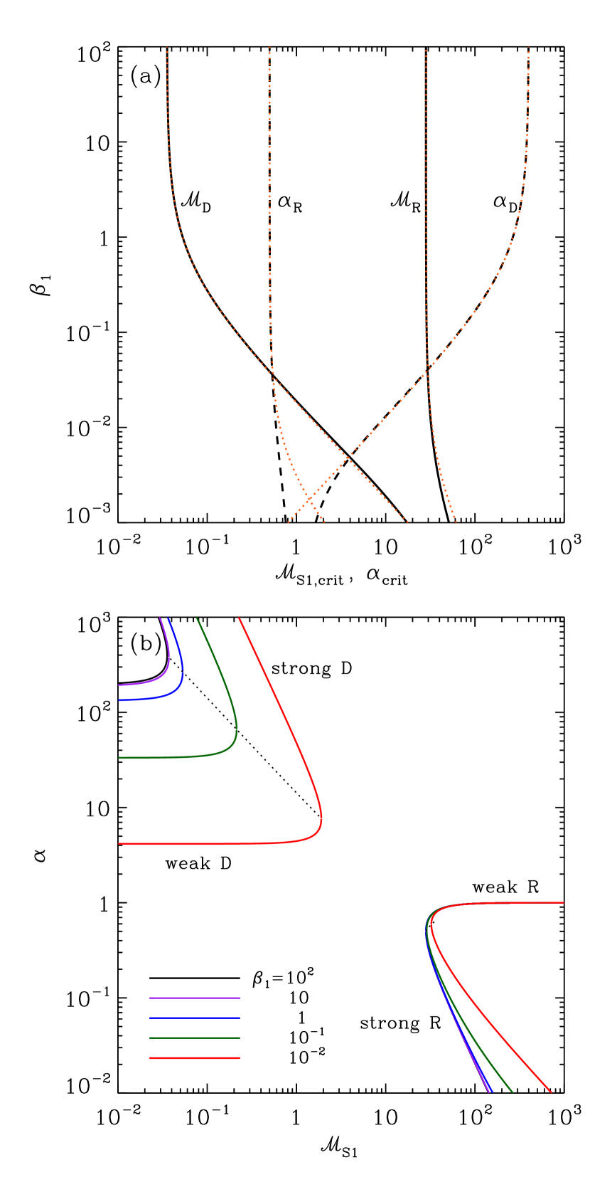
Figure 1: (a) Dependence on $\beta_{1}$ of the critical Mach numbers $\mathcal{M}_{\rm D}$ and $\mathcal{M}_{\rm R}$ (black solid lines) and the critical expansion factors $\alpha_{\rm D}$ and $\alpha_{\rm R}$ (black dashed lines) for $\theta=200$. The red dotted lines give the analytic approximations (Equations (27) and (28)). (b) Expansion factors $\alpha$ of magnetic IFs with $\theta=200$ for various $\beta_{1}$. The dotted curves mark the loci of the critical fronts where strong and weak solutions merge.

Figure 1(a) plots the relationships between $\beta_{1}$ and $\mathcal{M}_{\rm S1,crit}$ (black solid lines) and between $\beta_{1}$ and $\alpha_{\rm crit}$ (black dashed lines) for $\theta=200$. Clearly, $\mathcal{M}_{\rm D}$ and $\mathcal{M}_{\rm R}$ are close to the unmagnetized value given in Equation (19) for $\beta_{1}\lower 2.15277pt\hbox{$\;\buildrel>\over{\sim}\;$}10$. They increase as $\beta_{1}$ decreases. For $\theta\gg 1$ and $\beta_{1}\theta\gg 1$, one can expand Equations (26) relative to the unmagnetized solutions to show that the critical expansion factors are approximately

$$\begin{split}\alpha_{\rm D}&\approx 2\theta\left(1+\frac{1}{2\beta_{1}}\right)^{-1}\,,\\ \alpha_{\rm R}&\approx\frac{1}{2}+\frac{5}{16\theta\beta_{1}}\,.\end{split}$$ (27)

The corresponding critical Mach numbers are

$$\begin{split}\mathcal{M}_{\rm D}^{2}&\approx\frac{1}{4\theta}\left(1+\frac{1}{2\beta_{1}}\right)^{2},\\ \mathcal{M}_{\rm R}^{2}&\approx 4\theta\left(1+\frac{3}{4\beta_{1}\theta}\right).\end{split}$$ (28)

These are plotted as red dotted lines in Figure 1(a), in good agreement with the full solutions for $\beta_{1}\lower 2.15277pt\hbox{$\;\buildrel>\over{\sim}\;$}10^{-2}$.

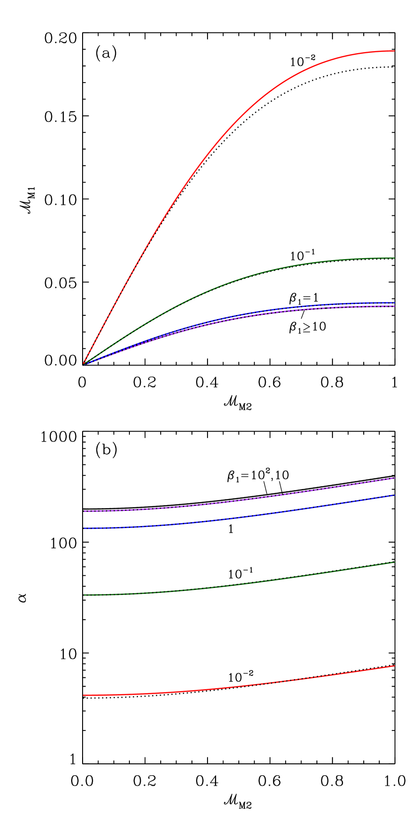
Figure 2: Dependence of (a) the upstream magnetosonic Mach number $\mathcal{M}_{\rm{M}1}$ and (b) the expansion factor $\alpha$ on the downstream magnetosonic Mach number $\mathcal{M}_{\rm{M}2}$ for weak D-type IFs with $\theta=200$. The solid lines give the full numerical results, while the dotted lines draw the approximate solutions (Equations (29) and (30)).

Figure 1(b) plots the expansion factors of magnetized IFs for different values of $\beta_{1}$ as functions of $\mathcal{M}_{\rm{S1}}$ for $\theta=200$. The dotted lines draw the loci of the D- and R-critical IFs. Weak R-type IFs have $\alpha\approx 1$, and their physical conditions are almost unaffected by the presence of magnetic fields (Lasker, 1966). For weak D-type IFs displayed in the lower parts of the left curves, however, magnetic fields lower the expansion factor considerably, especially for $\beta_{1}\lesssim 1$.

Figure 2 plots $\mathcal{M}_{\rm{M}1}$ and $\alpha$ as functions of $\mathcal{M}_{\rm{M}2}$ for weak D-type IFs with $\theta=200$. Magnetic fields clearly reduce $\alpha$, while increasing $\mathcal{M}_{\rm{M}1}$ for given $\mathcal{M}_{\rm{M}2}$. Since $\mathcal{M}_{\rm{S1}}^{2}\ll 1$ and $\beta_{2}\gg 1$ for weak D-type IFs, Equation (8) approximately gives

$$\alpha\approx\theta\dfrac{1+\mathcal{M}_{\rm{S2}}^{2}}{1+1/(2\beta_{1})}\approx\theta\dfrac{1+\mathcal{M}_{\rm{M}2}^{2}}{1+1/(2\beta_{1})}\,,$$ (29)

which, combined with Equation (16), yields

$$\mathcal{M}_{\rm{M}1}\approx\frac{1}{\theta^{1/2}}\dfrac{1+1/(2\beta_{1})}{(1+\beta_{1}^{-1})^{1/2}}\dfrac{\mathcal{M}_{\rm{M}2}}{1+\mathcal{M}_{\rm{M}2}^{2}}\,,$$ (30)

These are plotted in Figure 2 as dotted lines, in good agreement with the full solutions (better than 6% for $\beta_{1}\geq 10^{-2}$). Note that the second approximation in Equation (29) follows from the approximation $\beta_{2}\gg 1$, which is usually the case unless $\beta_{1}\theta\lesssim 1$ (see Equation (14) and Figure 2). Equation (29) then indicates that the magnetic fields reduce the expansion factor $\alpha$ by a factor of $1+1/(2\beta_{1})$ compared to the unmagnetized value.

3 Perturbation Equations

We now apply small-amplitude perturbations to a steady IF with $\boldsymbol{v}_{\rm A}=v_{\rm A}\hat{\mathbf{x}}$ found in the preceding section, and then explore their stability. Since the background flow is uniform except at $z=0$, Equations (1)–(5) can be linearized on both sides of the front as

$$\left(\dfrac{\partial}{\partial t}+\boldsymbol{v}\cdot\nabla\right)\rho^{\prime}=-\rho\nabla\cdot\boldsymbol{v}^{\prime}\,,$$ (31)

$$\left(\dfrac{\partial}{\partial t}+\boldsymbol{v}\cdot\nabla\right)\boldsymbol{v}^{\prime}=-\dfrac{1}{\rho}\nabla\left(P^{\prime}+\dfrac{\boldsymbol{B}\cdot\boldsymbol{B}^{\prime}}{4\pi}\right)+\dfrac{1}{4\pi\rho}(\boldsymbol{B}\cdot\nabla)\boldsymbol{B}^{\prime}\,,$$ (32)

$$\left(\dfrac{\partial}{\partial t}+\boldsymbol{v}\cdot\nabla\right)\boldsymbol{B}^{\prime}=(\boldsymbol{B}\cdot\nabla)\boldsymbol{v}^{\prime}-\boldsymbol{B}(\nabla\cdot\boldsymbol{v}^{\prime})\,,$$ (33)

$$\nabla\cdot\boldsymbol{B}^{\prime}=0\,,$$ (34)

$$P^{\prime}=c_{\rm s}^{2}\rho^{\prime}\,,$$ (35)

where the primes denote the perturbed quantities. We assume that the perturbations vary in space and time as

$$\propto\exp(i\boldsymbol{k}\cdot\boldsymbol{x}+\Omega t)\,,$$ (36)

where $\boldsymbol{k}=(k_{x},k_{y},k_{z})$ and $\Omega$ are the wavenumber and the frequency of the perturbations, respectively. We take a convention that $k_{x}$ and $k_{y}$ are real, while $\Omega$ and $k_{z}$ are complex.

Equations (31)–(35) are then reduced to

$$\Omega_{D}\rho^{\prime}=-\rho(i\boldsymbol{k}\cdot\boldsymbol{v}^{\prime})\,,$$ (37)

$$\Omega_{D}\boldsymbol{v}^{\prime}=-i\boldsymbol{k}\left(\frac{c_{\rm s}^{2}}{\rho}\rho^{\prime}+v_{\rm A}b_{x}^{\prime}\right)+ik_{x}v_{\rm A}\boldsymbol{b}^{\prime}\,,$$ (38)

$$\Omega_{D}\boldsymbol{b}^{\prime}=ik_{x}v_{\rm A}\boldsymbol{v}^{\prime}-iv_{\rm A}(\boldsymbol{k}\cdot\boldsymbol{v}^{\prime})\hat{\mathbf{x}}\,,$$ (39)

$$\boldsymbol{k}\cdot\boldsymbol{b}^{\prime}=0\,,$$ (40)

where $\Omega_{D}\equiv\Omega+ik_{z}v_{z}$ is the Doppler-shifted frequency and $\boldsymbol{b}^{\prime}\equiv\boldsymbol{B}^{\prime}/\sqrt{4\pi\rho}$ has the units of velocity. Equations (37)–(40) are combined to yield

$$\begin{split}(\Omega_{D}^{2}+k_{x}^{2}v_{\rm A}^{2})\boldsymbol{v}^{\prime}+[(c_{\rm s}^{2}+v_{\rm A}^{2})(\boldsymbol{k}\cdot\boldsymbol{v}^{\prime})-k_{x}v_{\rm A}^{2}v_{x}^{\prime}]\boldsymbol{k}-k_{x}v_{\rm A}^{2}(\boldsymbol{k}\cdot\boldsymbol{v}^{\prime})\hat{\mathbf{x}}=0\,,\end{split}$$ (41)

(e.g., Lithwick & Goldreich, 2001). This is a generic dispersion relation for waves in a uniform medium moving at a constant velocity.

3.1 Canonical Modes

As is well known, Equation (41) gives algebraic relations for three different kinds of propagating waves: Alfvén, fast, and slow waves (e.g., Shu, 1992). In this subsection, we derive the dispersion relation of each mode and the corresponding eigenvector with arbitrary normalization, in a form suitable for our perturbation analysis.

3.1.1 Shear Alfvén modes

Shear Alfvén waves are transverse waves with $\boldsymbol{k}\cdot\boldsymbol{v}^{\prime}=0$, for which Equation (41) is reduced to

$$\Omega_{D}^{2}+k_{x}^{2}v_{\rm A}^{2}=0\,.$$ (42)

It then follows from Equations (37)–(39) that $\boldsymbol{b}^{\prime}=\pm\boldsymbol{v}^{\prime}$, $(\boldsymbol{k}\cdot\boldsymbol{v}^{\prime})=(\boldsymbol{k}\cdot\boldsymbol{b}^{\prime})=0$, and $v_{x}^{\prime}=b_{x}^{\prime}=0$, indicating that Alfvén waves are incompressible and thus do not rely on thermal pressure. The eigenvector of shear Alfvén waves is thus

$$P^{\prime}=0\,,$$ (43)

$$\boldsymbol{v}^{\prime}=(0,k_{z},-k_{y})\,,$$ (44)

$$\boldsymbol{b}^{\prime}=(0,\pm k_{z},\mp k_{y})\,,$$ (45)

where the signs distinguish two oppositely propagating waves. As we will explain below, shear Alfvén waves with $k_{z}\neq 0$ are not excited by the distortions of an IF that we impose and thus out of consideration in our analysis.

3.1.2 Fast and Slow modes

When both the magnetic forces and the thermal pressure are important, we take the scalar product of Equation (41) with $\boldsymbol{k}$ and $\boldsymbol{v}_{\rm A}$. This results in two homogeneous linear equations for $(\boldsymbol{k}\cdot\boldsymbol{v}^{\prime})$ and $(\boldsymbol{v}_{\rm A}\cdot\boldsymbol{v}^{\prime})$. The condition for the existence of non-trivial solutions yields

$$\Omega_{D}^{4}+k^{2}(c_{\rm s}^{2}+v_{\rm A}^{2})\Omega_{D}^{2}+k_{x}^{2}k^{2}c_{\rm s}^{2}v_{\rm A}^{2}=0\,,$$ (46)

where $k=(k_{x}^{2}+k_{y}^{2}+k_{z}^{2})^{1/2}$. This is a usual dispersion relation for fast and slow MHD waves, for which $\boldsymbol{v}_{\rm A}$, $\boldsymbol{v}^{\prime}$, and $\boldsymbol{k}$ lie in the same plane. We use Equations (37)–(40) to write the perturbed quantities in terms of $v_{z}^{\prime}$ as

$$\frac{P^{\prime}}{\rho}=-\frac{(\Omega_{D}^{2}+k^{2}v_{\rm A}^{2})}{ik_{z}\Omega_{D}}v_{z}^{\prime}\,,$$ (47)

$$\boldsymbol{v}^{\prime}=\left(\frac{k_{x}(\Omega_{D}^{2}+k^{2}v_{\rm A}^{2})}{k_{z}\Omega_{D}^{2}},\frac{k_{y}}{k_{z}},1\right)v_{z}^{\prime}\,,$$ (48)

$$\boldsymbol{b}^{\prime}=\left(\frac{-i(k_{y}^{2}+k_{z}^{2})v_{\rm A}}{k_{z}\Omega_{D}},\frac{ik_{x}k_{y}v_{\rm A}}{k_{z}\Omega_{D}},\frac{ik_{x}v_{\rm A}}{\Omega_{D}}\right)v_{z}^{\prime}\,,$$ (49)

for $\Omega_{D}\neq 0$ and $k_{z}\neq 0$. Note that the eigenvectors of fast and slow modes with $\Omega_{D}\neq 0$ can be completely specified by assigning one variable (e.g., $v_{z}^{\prime}$).

Equation (46) has a special slow mode with $\Omega_{D}=0$, occurring when $k_{x}v_{\rm A}=0$ (for $k\neq 0$). Equations (37)–(40) then give

$$k_{y}v_{y}^{\prime}+k_{z}v_{z}^{\prime}=0\,,$$ (50)

and

$$\dfrac{P^{\prime}}{\rho}+v_{\rm A}b_{x}^{\prime}=0\,.$$ (51)

This corresponds to vortex modes, requiring no perturbation in the total pressure. These modes are generated at a curved IF and then simply advected downstream from the front. Although Equation (51) is a general expression for the perturbed pressure of the vortex modes, the perturbations we consider in the present work require that $P^{\prime}=b_{x}^{\prime}=0$ (see Section 5.1).

For later purposes, we introduce the following dimensionless quantities:

$$\sigma\equiv\frac{\Omega}{v_{z1}(k_{x}^{2}+k_{y}^{2})^{1/2}}\,,\;\;\;\nu\equiv\frac{ik_{z}}{(k_{x}^{2}+k_{y}^{2})^{1/2}}\,,\;\;\;\cos\psi\equiv\frac{k_{x}}{(k_{x}^{2}+k_{y}^{2})^{1/2}}\,.$$ (52)

Equation (46) can then be expressed as

$$\mathcal{M}_{\rm{M}}^{2}\sigma_{D}^{4}+\hat{\alpha}^{2}(1-\nu^{2})\sigma_{D}^{2}+\hat{\alpha}^{4}(1-\nu^{2})\frac{\cos^{2}\psi}{(1+\beta^{-1})\mathcal{M}_{\rm{A}}^{2}}=0\,,$$ (53)

where $\sigma_{D}=\sigma+\hat{\alpha}\nu$, and $\hat{\alpha}\equiv v_{z}/v_{z1}=1$ in the upstream side and $\hat{\alpha}=\alpha$ in the downstream side.

3.2 Perturbed Jump Conditions

Perturbations given in Equation (36) result from sinusoidal distortions of an IF which would otherwise remain planar. Since the IF involves discontinuities of fluid quantities, there are certain conditions that the perturbation variables should obey at the perturbed IF. Let the shape of a deformed IF be described by

$$\mathcal{F}(x,y,z,t)=z-\zeta e^{\Omega t+ik_{x}x+ik_{y}y}=0\,,$$ (54)

where $\zeta\,(\ll k^{-1})$ denotes the amplitude of the IF distortion. Then, the unit vector normal to the perturbed front is given by $\hat{\mathbf{n}}=\nabla\mathcal{F}/|\nabla\mathcal{F}|=\hat{\mathbf{z}}-ik_{x}\zeta\hat{\mathbf{x}}-ik_{y}\zeta\hat{\mathbf{y}}$, while the two unit vectors tangential to the front can be chosen as $\hat{\mathbf{t}}_{\rm a}=\hat{\mathbf{x}}+ik_{x}\zeta\hat{\mathbf{z}}$ and $\hat{\mathbf{t}}_{\rm b}=\hat{\mathbf{y}}+ik_{y}\zeta\hat{\mathbf{z}}$, to the first order in $k\zeta$.

It is straightforward to show that in the frame comoving with the perturbed IF, the velocity components parallel to $\hat{\mathbf{n}}$, $\hat{\mathbf{t}}_{\rm a}$, and $\hat{\mathbf{t}}_{\rm b}$ are given by

$$v_{\rm n}=v_{z}+v_{z}^{\prime}-\zeta\Omega\,,$$ (55)

$$\mathbf{v}_{\rm t}=(v_{x}^{\prime}+ik_{x}\zeta v_{z},v_{y}^{\prime}+ik_{y}\zeta v_{z})\,,$$ (56)

respectively. Similar expressions for the magnetic fields read

$$B_{\rm n}=B_{z}^{\prime}-ik_{x}\zeta B_{x}\,,$$ (57)

$$\mathbf{B}_{\rm t}=(B_{x}+B_{x}^{\prime},B_{y}^{\prime})\,,$$ (58)

respectively.

Equations (1)–(3) can be recast into flux-conservative form and integrated over the small volume located on the front. By applying the divergence theorem, we obtain the following set of jump conditions

$$\Delta\left[\rho v_{\rm n}\right]=0\,,$$ (59)

$$\Delta\left[\rho v_{\rm n}\mathbf{v}_{\rm t}-\dfrac{B_{\rm n}\mathbf{B}_{\rm t}}{4\pi}\right]=0\,,$$ (60)

$$\Delta\left[\rho v_{\rm n}^{2}+P+\dfrac{B^{2}_{\rm t}}{8\pi}\right]=-\Delta\left[\rho\right]g\zeta\,,$$ (61)

$$\Delta\left[v_{\rm n}\mathbf{B}_{\rm t}-B_{\rm n}\mathbf{v}_{\rm t}\right]=0\,,$$ (62)

and

$$\Delta\left[B_{\rm n}\right]=0\,,$$ (63)

(see, e.g., Shu 1992). Here, $\Delta[f]\equiv f(z=\zeta+0)-f(z=\zeta-0)=f_{2}-f_{1}$ indicates the difference of a quantity $f$ evaluated at immediately behind and ahead of the front.

Substituting Equations (55)–(58) in Equations (59)–(63), one can show that the zeroth-order terms lead to Equations (7)–(9). Taking the first-order terms, one obtains

$$\Delta\left[\rho^{\prime}v_{z}+\rho(v_{z}^{\prime}-\Omega\zeta)\right]=0\,,$$ (64)

$$\Delta\left[\rho v_{z}(v_{x}^{\prime}+ik_{x}\zeta v_{z})-\rho v_{\rm A}(b_{z}^{\prime}-ik_{x}\zeta v_{\rm A})\right]=0\,,$$ (65)

$$\Delta\left[\rho v_{z}(v_{y}^{\prime}+ik_{y}\zeta v_{z})\right]=0\,,$$ (66)

$$\Delta\left[\rho^{\prime}v_{z}^{2}+2\rho v_{z}(v_{z}^{\prime}-\Omega\zeta)+\rho v_{z}p^{\prime}+\rho v_{\rm A}b_{x}^{\prime}\right]=-\Delta\left[\rho\right]g\zeta\,,$$ (67)

$$\Delta\left[\rho^{1/2}(b_{x}^{\prime}v_{z}+v_{\rm A}(v_{z}^{\prime}-\Omega\zeta))\right]=0\,,$$ (68)

$$\Delta\left[\rho^{1/2}b_{y}^{\prime}v_{z}\right]=0\,,$$ (69)

$$\Delta\left[\rho^{1/2}(b_{z}^{\prime}-ik_{x}\zeta v_{\rm A})\right]=0\,,$$ (70)

where $p^{\prime}=P^{\prime}/(\rho v_{z})$. Note that only two among Equations (68)–(70) are independent since the induction equation automatically satisfies the divergence-free condition for magnetic fields. Therefore, the perturbed jump conditions at the front provide six constraints for the perturbation variables.

An additional constraint can be obtained by linearizing Equation (6) as

$$\rho_{1}^{\prime}v_{z1}+\rho_{1}(v_{z1}^{\prime}-\Omega\zeta)=m_{\rm{H}}F_{\rm ph}^{\prime}\,,$$ (71)

where $F_{\rm ph}^{\prime}$ is the perturbed photon flux at the distorted IF. For simplicity, we set $F_{\rm ph}^{\prime}=0$ in the present work, implying that the mass flux per unit area through the IF is unchanged in the perturbed state. We note that $F_{\rm ph}^{\prime}$ can be non-vanishing when the effect of finite probability for photon absorption in the ionized region is considered, suppressing the instability at scales larger than the recombination length scale (see Axford 1964; Williams 2002).

Defining $Z\equiv\zeta(k_{x}^{2}+k_{y}^{2})^{1/2}v_{z1}$ and $G\equiv g/((k_{x}^{2}+k_{y}^{2})^{1/2}v_{z1}^{2})$, Equations (64)–(69) and (71) can be simplified as

$$\mathcal{M}_{\rm{S1}}^{2}p_{1}^{\prime}+v_{z1}^{\prime}-\sigma Z=0\,,$$ (72)

$$\mathcal{M}_{\rm{S2}}^{2}p_{2}^{\prime}+v_{z2}^{\prime}-\sigma Z=0\,,$$ (73)

$$v_{x1}^{\prime}-\mathcal{M}_{\rm{A1}}^{-1}b_{z1}^{\prime}-v_{x2}^{\prime}+\mathcal{M}_{\rm{A2}}^{-1}b_{z2}^{\prime}+i(1+\mathcal{M}_{\rm{A1}}^{-2}-\alpha(1+\mathcal{M}_{\rm{A2}}^{-2}))\cos\psi Z=0\,,$$ (74)

$$v_{y1}^{\prime}-v_{y2}^{\prime}+i(1-\alpha)\sin\psi Z=0\,,$$ (75)

$$\left((1+\beta_{1}^{-1})(1-\mathcal{M}_{\rm{M}1}^{2})+\cos^{2}\psi\dfrac{\mathcal{M}_{\rm{A1}}^{-2}(1-\alpha^{-2})}{(\sigma+\nu)^{2}}\right)p_{1}^{\prime}-(1+\beta_{2}^{-1})(1-\mathcal{M}_{\rm{M}2}^{2})p_{2}^{\prime}+(1-\alpha^{-1})GZ=0\,,$$ (76)

$$b_{x1}^{\prime}-\mathcal{M}_{\rm{A1}}^{-1}\mathcal{M}_{\rm{S1}}^{2}p_{1}^{\prime}-\alpha^{1/2}\left(b_{x2}^{\prime}-\mathcal{M}_{\rm{A2}}^{-1}\mathcal{M}_{\rm{S2}}^{2}p_{2}^{\prime}\right)=0\,,$$ (77)

$$b_{y1}^{\prime}-\alpha^{1/2}b_{y2}^{\prime}=0\,.$$ (78)

Of the equations above, the derivation of Equation (76) is not trivial, requiring to utilize Equations (46)–(49): we present the necessary steps for it in Appendix A.

4 Instability of Unmagnetized IFs

We now want to explore the instability of an isolated, weak D-type IF. Here, the term “isolated” implies that disturbances are generated only at the front and decay at a large distance from the front. Of the MHD waves described above, therefore, we consider only waves that are evanescent away from the front, i.e., ${\rm Im}(k_{z})<0$ in the upstream side ($z<0$) and ${\rm Im}(k_{z})>0$ in the downstream side ($z>0$), which is imposed by the regularity condition at infinity. In our method, finding the growth rate as well as the eigenstate of unstable modes takes two steps: (1) we express the perturbation variables as a linear superposition of the canonical waves at each side of the perturbed IF; (2) we then require the perturbation variables to fulfill the jump conditions at the perturbed IF.

Vandervoort (1962) was the first who studied the instability of unmagnetized IFs. In this section, we revisit the problem to exemplify our technique in the most simplest case, and to elucidate the physical nature of the instability in analogy to the DLI. The case of magnetized IFs will be presented in Section 5.

In the absence of magnetic fields, the background flows possess rotational symmetry with respect to the $z$-axis, so that we may take $k_{y}=0$ (hence $\cos\psi=1$) and $v_{y}^{\prime}=0$ without any loss of generality. The solutions of Equation (53) in the limit of $\mathcal{M}_{\rm{A}}$, $\beta\rightarrow\infty$ are

$$\nu_{\rm{a}}=\dfrac{1}{1-\mathcal{M}_{\rm{S}}^{2}}\left[\mathcal{M}_{\rm{S}}^{2}\dfrac{\sigma}{\hat{\alpha}}\pm\sqrt{\mathcal{M}_{\rm{S}}^{2}\left(\frac{\sigma^{2}}{\hat{\alpha}^{2}}-1\right)+1}\right]\,,$$ (79)

$$\nu_{\rm{v}}=-{\sigma}/{\hat{\alpha}}\,,$$ (80)

where the subscripts “a” and “v” stand for acoustic and vortex modes, respectively, which are only modes that constitute the perturbations at each side of the IF. Since the vortex mode is produced by the front deformation and then passively advected by the background flows, it exists only in the downstream side.

Let $\mathbf{S}=(p^{\prime},\,v_{x}^{\prime},\,v_{z}^{\prime})$ describe the eigenvectors of the canonical waves such that

$$\mathbf{S}_{\rm{a}}=\left(-1-{\sigma}/{(\hat{\alpha}\nu_{\rm{a}})}\,,{i}/{\nu_{\rm{a}}},\,1\right),\,$$ (81)

and

$$\mathbf{S}_{\rm{v}}=\left(0,\,-i\sigma/\alpha,\,1\right)\,.$$ (82)

The boundary conditions for isolated IFs require that $\rm{Re}(\nu_{\rm{a}})>0$ in the upstream neutral region, while $\rm{Re}(\nu_{\rm{a}})<0$ in the downstream ionized region, as mentioned above. For unstable modes with $\rm{Re}(\sigma)>0$ and $\mathcal{M}_{\rm{S}}^{2}<1$, one can write the total perturbations as a linear combination of the canonical modes as

$$\mathbf{S}_{1}=C_{\rm a1}\mathbf{S}_{\rm{a1}}\,,$$ (83)

in the upstream side, and

$$\mathbf{S}_{2}=C_{\rm a2}\mathbf{S}_{\rm{a2}}+C_{\rm v2}\mathbf{S}_{\rm{v2}}\,,$$ (84)

in the downstream side. Here, $C_{\rm a1}$, $C_{\rm a2}$, and $C_{\rm v2}$ are the coefficients to be determined, and $\nu_{\rm{a}}$ in Equation (79) should be calculated with the positive and negative signs for $\mathbf{S}_{\rm{a1}}$ and $\mathbf{S}_{\rm{a2}}$, respectively.

Plugging Equations (83) and (84) into Equations (72)–(74) and (76) for $v_{\rm A}=0$, we are left with a set of linear equations for four variables $(C_{\rm a1},C_{\rm a2},C_{\rm v2},Z)$. These can be cast into a matrix form as

$${\small\left(\begin{array}[]{cccc}1-\mathcal{M}_{\rm{S1}}^{2}\left(1+\sigma/\nu_{\rm{a1}}\right)&0&0&-\sigma\\ 0&1-\mathcal{M}_{\rm{S2}}^{2}\left(1+\sigma/(\alpha\nu_{\rm{a2}})\right)&1&-\sigma\\ \nu_{\rm{a1}}^{-1}&-\nu_{\rm{a2}}^{-1}&\sigma/\alpha&1-\alpha\\ -(1-\mathcal{M}_{\rm{S1}}^{2})\left(1+\sigma/\nu_{\rm{a1}}\right)&(1-\mathcal{M}_{\rm{S2}}^{2})\left(1+\sigma/(\alpha\nu_{\rm{a2}})\right)&0&(1-\alpha^{-1})G\end{array}\right)\left(\begin{array}[]{c}C_{\rm a1}\\ C_{\rm a2}\\ C_{\rm v2}\\ Z\end{array}\right)=0\,.}$$ (85)

In order to have a nontrivial solution, the $4\times 4$ matrix in Equation (85) must have a vanishing determinant. This yields

$$(\sigma-\Gamma_{2}\alpha)\left[1+\Gamma_{1}\left(\dfrac{\sigma}{\alpha}-\dfrac{\alpha-1}{\sigma}\right)\right]=(\alpha-\Gamma_{2}\sigma)\left[\sigma+\Gamma_{1}\left(1+\dfrac{1-\alpha}{\alpha}\dfrac{G}{\sigma}\right)\right]\,,$$ (86)

where

$$\Gamma_{1}=[1+\mathcal{M}_{\rm{S1}}^{2}(\sigma^{2}-1)]^{1/2}\,,$$ (87)

$$\Gamma_{2}=\left[1+\mathcal{M}_{\rm{S2}}^{2}(\sigma^{2}/\alpha^{2}-1)\right]^{1/2}\,,$$ (88)

which is our desired dispersion relation for instability of unmagnetized IFs. Note that Equation (86) is the same as Equation (79) of Vandervoort (1962, see also ) when the direction of radiation is normal to the front.

In the incompressible limit of $\mathcal{M}_{\rm{S}}\rightarrow 0$, Equation (86) reduces to

$$\sigma=\dfrac{\alpha}{\alpha+1}\left(\sqrt{1+\alpha-\frac{1}{\alpha}+\dfrac{\alpha^{2}-1}{\alpha^{2}}G}-1\right)\,.$$ (89)

In more general, compressible cases, however, Equation (86) does not provide a closed-form expression for $\sigma$. Although it can be converted to a polynomial by repeated squaring (e.g., Sysoev, 1997), the resulting 16-th order polynomial in $\sigma$ is not so illuminating that we present only the numerical results here. Figure 3(a) plots as solid lines the dimensionless growth rate $\sigma$ as a function of $\mathcal{M}_{\rm{S2}}$ for $\theta=100$, $200$, and $300$, when $G=0$. For fixed $\theta$, $\sigma$ increases slightly with increasing $\mathcal{M}_{\rm{S2}}\lower 2.15277pt\hbox{$\;\buildrel<\over{\sim}\;$}0.7$ due to the increase in $\alpha$ (see Figure 2(b) and Equation (89)). As $\mathcal{M}_{\rm{S2}}$ increases further, $\sigma$ starts to decrease and tends to zero at $\mathcal{M}_{\rm{S2}}=1$ corresponding to the D-critical front. Figure 3(a) also plots as dashed line $\sigma$ for $\alpha=100$, 200, and 300, showing that $\sigma$ monotonically decreases with increasing $\mathcal{M}_{\rm{S2}}$ for fixed $\alpha$. This suggests that the stabilization of the IF instability is caused by gas compressibility, as we will explain below.

Note that the incompressible dispersion of Equation (89) with $G=0$ is identical to the dispersion relation of the DLI of an evaporation front in an incompressible fluid (e.g., Zeldovich et al., 1985; Inoue et al., 2006; Kim & Kim, 2013). Furthermore, Equation (86) is equal to the full dispersion relation of the DLI when the effect of compressibility is included (Bychkov et al., 2008). This suggests that the physical nature of the instability of an IF is the same as that of the DLI. When an IF is disturbed, the gas expansion across the front makes the pressure drop (rise) on the part of the distorted IF convex (concave) toward the ionizing source. The changes in the pressure induce gas motions such that more (less) neutral gas is directed toward to the convex (concave) parts. Since the ionizing photon flux at the IF is assumed to be fixed, this makes the convex (concave) parts advance further toward (recede away from) the ionizing source in a runaway fashion, indicative of instability.

When gas compressibility is considered, the pressure drop (rise) is partly translated into the drop (rise) in the perturbed density via $\rho^{\prime}/\rho\sim\mathcal{M}_{\rm{S}}^{-2}P^{\prime}/P$. This causes less changes in the perturbed velocities compared to the incompressible limit. Consequently, the amount of the perturbed mass flux at the distorted IF is reduced, making the instability grow at a slower rate. For the D-critical IF with $\mathcal{M}_{\rm{S2}}=1$, the perturbations in the downstream side are unable to propagate into the upstream side since the ionized gas is advected at the sound speed. Accordingly, the neutral gas does not respond to the deformation of the IF and remains unperturbed. This can be seen more quantitatively from Equation (76) which gives $p_{1}^{\prime}=0$ when $G=0$, which in turn gives $C_{\rm a1}=0$ in Equation (83) hence $\sigma=0$ from Equation (72).

Figure 3(b) plots $\sigma$ for $\theta=200$ and differing $G$, showing the positive $G$ corresponding to an accelerating front make the front more unstable. When the term involving $G$ dominates, Equation (89) recovers the growth rate of the RTI. When $G>0$, therefore, the DLI and RTI cooperate constructively. For decelerating IFs with $G<0$, on the other hand, large scale modes with $kv_{z1}^{2}/|g|<\alpha$ are suppressed by buoyancy. The instability is completely quenched by buoyancy, provided

$$G<-\alpha(1-\mathcal{M}_{\rm{S2}}^{2})^{1/2}\,,$$ (90)

which can be obtained by imposing $\sigma\rightarrow 0$ in Equation (86).

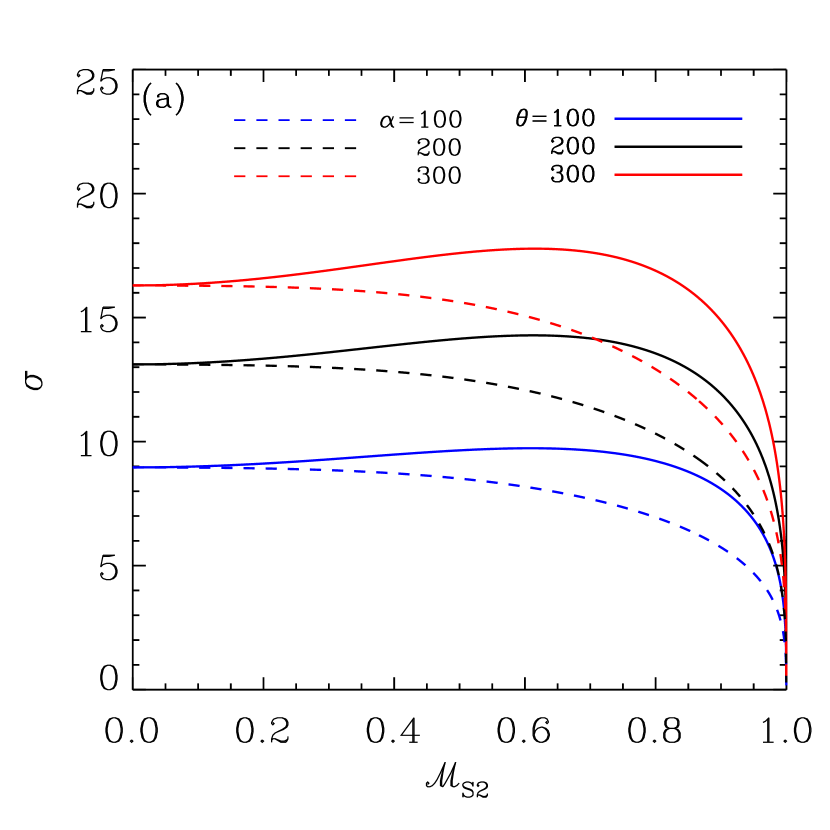
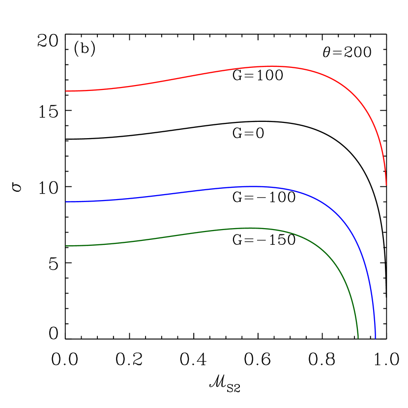
Figure 3: (a) Dimensionless growth rate $\sigma$ of the instability of unmagnetized IFs as a function of the downstream sonic Mach number $\mathcal{M}_{\rm{S2}}$ for fixed heating factor $\theta$ (solid lines) and for fixed expansion factor $\alpha$ (dashed lines) with $G=0$. (b) Dependence of $\sigma$ on $G$ for $\theta=200$. Accelerating fronts with larger $G$ are more unstable.

5 Instability of Magnetized IFs

For the stability of magnetized IFs, we consider only two types of perturbations: (1) perturbations with $k_{x}=0$ and $k_{y}\neq 0$ (i.e., $\cos\psi=0$) and (2) perturbations with $k_{x}\neq 0$ and $k_{y}=0$ (i.e., $\cos\psi=1$). While these perturbations are not most general, they can nevertheless capture the essential physics of magnetic fields in the IF instability.

5.1 Cases with $k_{x}=0$ and $k_{y}\neq 0$

Perturbations with $k_{x}=0$ and $k_{y}\neq 0$ do not bend the field lines. Since the front deformation does not involve the $x$-direction, we only need to consider motions in the $y$-$z$ plane (i.e., $v_{x}^{\prime}=0$). Equations (39) then gives $b_{y}^{\prime}=b_{z}^{\prime}=0$, implying that the perturbed magnetic fields exert magnetic pressure only in the propagation direction of the disturbances and that shear Alfvén waves are not excited.

For $\cos\psi=0$, Equation (53) has two solutions

$$\nu_{\rm{f}}=\dfrac{1}{1-\mathcal{M}_{\rm{M}}^{2}}\left[\mathcal{M}_{\rm{M}}^{2}\dfrac{\sigma}{\hat{\alpha}}\pm\sqrt{\mathcal{M}_{\rm{M}}^{2}\left(\frac{\sigma^{2}}{\hat{\alpha}^{2}}-1\right)+1}\right]\,,$$ (91)

$$\nu_{\rm{s}}=-{\sigma}/{\hat{\alpha}}\,,$$ (92)

where the subscripts “f” and “s” stand for fast and slow modes, respectively. Note that Equation (91) is identical to Equation (79) provided $\mathcal{M}_{\rm{S}}$ is changed to $\mathcal{M}_{\rm{M}}$. Note also that Equation (92) is a dispersion relation for the magnetized vortex modes with $\Omega_{D}=0$, which exist only in the downstream side from the IF, as explained in Section 3.1.2.

Now, let $\mathbf{S}=(p^{\prime},\,v_{y}^{\prime},\,v_{z}^{\prime},\,b_{x}^{\prime})$ describe the eigenvectors of the basis modes. Then, Equations (47)–(49) give

$$\mathbf{S}_{\rm{f}}=\left[-\frac{1}{1+\beta^{-1}}\left(1+\dfrac{\sigma}{\hat{\alpha}\nu_{\rm{f}}}\right),\,\frac{i}{\nu_{\rm{f}}},1,-\frac{\mathcal{M}_{\rm{M}}^{2}}{\mathcal{M}_{\rm{A}}}\left(1+\dfrac{\sigma}{\hat{\alpha}\nu_{\rm{f}}}\right)\right]\,,$$ (93)

for the fast modes. On the other hand, the eigenvectors of the slow modes in the downstream side are given by

$$\mathbf{S}_{\rm{s2}}=(0,\,-i\sigma/\alpha,\,1,\,0)\,,$$ (94)

from Equation (50). Note that here we take $P^{\prime}=b_{x}^{\prime}=0$ from Equation (51) since $P^{\prime}$ and $b_{x}^{\prime}$ arising from the front distortions should have the same sign when $k_{x}=0$. Using the condition that the waves should decay far away from the IF, one can then write the state vectors as

$$\mathbf{S}_{1}=C_{\rm f1}\mathbf{S}_{\rm{f1}}\,,$$ (95)

$$\mathbf{S}_{2}=C_{\rm f2}\mathbf{S}_{\rm{f2}}+C_{\rm s2}\mathbf{S}_{\rm{s2}}\,,$$ (96)

where $C_{\rm f1}$, $C_{\rm f2}$, $C_{\rm s2}$ are coefficients to be determined.

Following the same steps as in the case of unmagnetized IFs, we apply the jump conditions (Equations (72), (73), (75), and (76)) to obtain a linear system of four equations in four unknowns $(C_{\rm f1},C_{\rm f2},C_{\rm s2},Z)$. From the condition for non-trivial solutions, we derive the dispersion relation for the instability of the magnetized IFs with $k_{x}=0$ and $k_{y}\neq 0$, which is identical to Equation (86), provided $\mathcal{M}_{\rm{S}}$ is replaced by $\mathcal{M}_{\rm{M}}$.

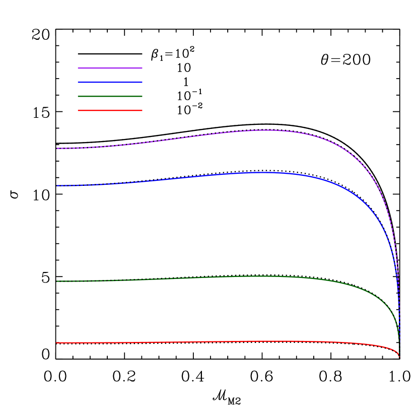
Figure 4: Growth rate of the instability of magnetized IFs with $\theta=200$ and differing $\beta_{1}$ as a function of $\mathcal{M}_{\rm{M}2}$, when the perturbations propagate perpendicular to the initial magnetic fields ($k_{x}=0$). The solid lines plot the full numerical results of the magnetized cases, while the dotted lines draw the hydrodynamic counterparts (Equation (86)) with $\alpha$ reduced by a factor of $1+1/(2\beta_{1})$.

Figure 4 plots as solid lines the dimensionless growth rate $\sigma$ for various $\beta_{1}$ when $\theta=200$ and $G=0$, as a function of $\mathcal{M}_{\rm{M}2}$. While the overall shape of the dispersion relations is unchanged compared to the hydrodynamics cases, magnetic fields certainly reduce $\sigma$. The dotted lines plot the unmagnetized dispersion relation, Equation (86), with $\alpha$ replaced by $\alpha/(1+1/(2\beta_{1}))$ which is the reduced expansion factor due to magnetic fields (e.g., Equation (29)). The good agreement between the solid and dotted lines suggests that the reduced growth rate in the magnetized case results simply from a decreased $\alpha$ in the background state. When $k_{x}=0$, magnetic fields remain straight and magnetized flows in the linear regime behave similarly to unmagnetized flows, with fast magnetosonic waves playing the exactly same role as acoustic waves.

5.2 Cases with $k_{x}\neq 0$ and $k_{y}=0$

We examine the stability of magnetized IFs with respect to perturbations lying in the $x$-$z$ plane, i.e., $k_{x}\neq 0$, $k_{y}=0$, and $v_{y}^{\prime}=b_{y}^{\prime}=0$, for which not only magnetic pressure but also magnetic tension affect the stability. Note that these requirements preclude the presence of shear Alfvén waves in the perturbations (e.g., Equations (44) and (45)). We first consider the incompressible limit and then generalize the results to compressible cases.

5.2.1 Incompressible Limit

For simplicity let us take the limit $c_{\rm s}\rightarrow\infty$ ($\rho^{\prime}=0$), while the Alfvén speed remains finite, so that $\beta\rightarrow\infty$ and $\mathcal{M}_{\rm{M}}\rightarrow 0$. Equation (53) with $\cos\psi=1$ then yields

$$\nu_{{\rm p}\pm}=\pm 1\,,$$ (97)

and

$$\nu_{{\rm s\pm}}=-{\sigma}/{\hat{\alpha}}\pm i\mathcal{M}_{\rm{A}}^{-1}\,,$$ (98)

where the subscripts “p” and “s” refer to the potential modes and slow (or pseudo-Alfvén) modes, respectively. The potential modes are a special case of the acoustic mode (or fast mode). For unstable modes with Re$(\sigma)>0$, it is apparent that the wave motions in the upstream side can be specified by the potential mode with $\nu_{{\rm p}+}=1$, while the other potential mode with $\nu_{{\rm p}-}=-1$ and two slow modes with $\nu_{{\rm s\pm}}$ (propagating in the opposite directions along the background magnetic fields) coexist in the downstream side.

Defining $\mathbf{S}=(p^{\prime},\,v_{x}^{\prime},\,v_{z}^{\prime},\,b_{x}^{\prime},\,b_{z}^{\prime})$, one can use Equations (37)–(40) to construct the eigenvector of each mode as

1. Upstream potential mode:

   $$\mathbf{S}_{\rm p1}=\left(-(\sigma+1),\,i,\,1,\,-\dfrac{\mathcal{M}_{\rm{A1}}^{-1}}{\sigma+1},\,\dfrac{i\mathcal{M}_{\rm{A1}}^{-1}}{\sigma+1}\right)\,,$$ (99)

2. Downstream potential mode:

   $$\mathbf{S}_{\rm p2}=\left(\dfrac{\sigma-\alpha}{\alpha},\,-i,\,1,\,-\dfrac{\alpha\mathcal{M}_{\rm{A2}}^{-1}}{\sigma-\alpha},\,\dfrac{i\alpha\mathcal{M}_{\rm{A2}}^{-1}}{\sigma-\alpha}\right)\,,$$ (100)

3. Downstream slow modes:

   $$\mathbf{S}_{\rm s2\pm}=\left(\mp i\mathcal{M}_{\rm{A2}}\nu_{{\rm s2\pm}},\,i\nu_{{\rm s2\pm}},\,1,\,\pm i\nu_{{\rm s2\pm}},\,\pm 1\right)\,,$$ (101)

where $\nu_{{\rm s2\pm}}$ is the value of $\nu_{{\rm s\pm}}$ in Equation (98) evaluated at the downstream side. The total perturbations are then given by

$$\mathbf{S}_{1}=C_{\rm p1}\mathbf{S}_{\rm p1}\,,$$ (102)

and

$$\mathbf{S}_{2}=C_{\rm p2}\mathbf{S}_{\rm p2}+C_{\rm s2+}\mathbf{S}_{\rm s2+}+C_{\rm s2-}\mathbf{S}_{\rm s2-}\,,$$ (103)

in the upstream and downstream sides, respectively.

Plugging these expressions into the perturbed jump conditions (Equations (72)–(74), (76), and (77)), one obtains a linear system of five equations in five unknowns $(C_{\rm p1},C_{\rm p2},C_{\rm s2+},C_{\rm s2-},Z)$, which is given in a matrix form by

$${\small\left(\begin{array}[]{ccccc}1&0&0&0&-\sigma\\ 0&1&1&1&-\sigma\\ 1-\dfrac{\mathcal{M}_{\rm{A1}}^{-2}}{\sigma+1}&1+\dfrac{\mathcal{M}_{\rm{A2}}^{-2}\alpha}{\sigma-\alpha}&-\nu_{{\rm s2+}}-i\mathcal{M}_{\rm{A2}}^{-1}&-\nu_{{\rm s2-}}+i\mathcal{M}_{\rm{A2}}^{-1}&1+\mathcal{M}_{\rm{A1}}^{-2}-\alpha(1+\mathcal{M}_{\rm{A2}}^{-2})\\ \mathcal{A}&-\dfrac{\sigma-\alpha}{\alpha}&i\mathcal{M}_{\rm{A2}}^{-1}\nu_{{\rm s2+}}&-i\mathcal{M}_{\rm{A2}}^{-1}\nu_{{\rm s2-}}&(1-\alpha^{-1})G\\ -\dfrac{\mathcal{M}_{\rm{A1}}^{-1}}{\sigma+1}&-\dfrac{\alpha^{3/2}\mathcal{M}_{\rm{A2}}^{-1}}{\sigma-\alpha}&-i\alpha^{1/2}\nu_{{\rm s2+}}&i\alpha^{1/2}\nu_{{\rm s2-}}&0\end{array}\right)\left(\begin{array}[]{c}C_{\rm p1}\\ C_{\rm p2}\\ C_{\rm s2+}\\ C_{\rm s2-}\\ Z\end{array}\right)=0\,,}$$ (104)

where $\mathcal{A}\equiv-(\sigma+1)\left[1+(1-\alpha^{-2})\mathcal{M}_{\rm{A1}}^{-2}/(\sigma+1)^{2}\right]$.

We set the determinant of the matrix to zero to obtain the dispersion relation

$$\sigma^{3}+\dfrac{3\alpha+1}{\alpha+1}\sigma^{2}-\dfrac{1}{\alpha(\alpha+1)}\left[\alpha^{3}-\left(3+\frac{1}{\mathcal{M}_{\rm{A1}}^{2}}-G\right)\alpha^{2}-G\alpha-\frac{1}{\mathcal{M}_{\rm{A1}}^{2}}\right]\sigma\\ -\dfrac{\alpha-1}{\alpha(\alpha+1)}\left[\alpha^{2}+\left(G-\frac{1}{\mathcal{M}_{\rm{A1}}^{2}}\right)\alpha+\mathcal{M}_{\rm{A1}}^{-2}\right]=0\,.$$ (105)

Note that Equation (105) is identical to Equation (112) of Dursi (2004), which is the dispersion relation for the incompressible DLI in a magnetized gas. This again demonstrates that the IF instability and the DLI share the common physical origin. In the limit of $\mathcal{M}_{\rm{A1}}\rightarrow\infty$, Equation (105) recovers Equation (89) in the unmagnetized case. On the other hand, we write Equation (105) in dimensional form and collect lowest-order terms in $v_{z1}$ to obtain

$$\Omega^{2}=gk_{x}\dfrac{\alpha-1}{\alpha+1}-k_{x}^{2}v_{\rm A1}^{2}\dfrac{1+\alpha^{2}}{\alpha(\alpha+1)}\,,$$ (106)

which is the usual dispersion relation for the RTI of a magnetized contact discontinuity, for which magnetic fields play a stabilizing role (e.g., Chandrasekhar, 1961).

Figure 5: Incompressible growth rate $\sigma$ of the instability of magnetized IFs as a function of the upstream Alfvénic Mach number $\mathcal{M}_{\rm{A1}}$, for in-plane perturbations with $k_{y}=0$. For given $\alpha$, $\sigma$ becomes smaller as the field strength increases (or $\mathcal{M}_{\rm{A1}}$ decreases). The instability is completely suppressed at sufficiently small $\mathcal{M}_{\rm{A1}}$ (see Equation (107)).

For given $\alpha$ and $\mathcal{M}_{\rm{A1}}$, Equation (105) has only one, if any, purely-growing solution with ${\rm Re}(\sigma)>0$ and ${\rm Im}(\sigma)=0$, while the other two correspond to decaying solutions. Figure 5 plots the growth rate of the unstable mode for various $\alpha$ as a function of $\mathcal{M}_{\rm{A1}}$, showing that $\sigma$ decreases as the field strength increases. It is a simple matter to show that the instability becomes completely suppressed, provided

$$\mathcal{M}_{\rm{A1}}<\sqrt{\dfrac{\alpha-1}{\alpha(\alpha+G)}},\,\,\,\text{for stability}\,.$$ (107)

The stabilization is due to magnetic tension forces that resist gas motions across the field lines. This can be seen more quantitatively as follows. The dimensionless growth rate with $v_{\rm A}=G=0$ in the incompressible limit is proportional to the fractional increase in the mass flux, i.e., $j_{z}^{\prime}/j_{z}=v_{z1}^{\prime}/v_{z1}=\sigma k_{x}\zeta\approx\sqrt{\alpha}k_{x}\zeta$ for $\alpha\gg 1$. The incoming velocity change $v_{z1}^{\prime}$ is due solely to the potential mode, which we denote by $v_{z,\rm{p}}^{\prime}$. On the other hand, the distorted front deforms the magnetic fields by an amount $B_{z}^{\prime}/B_{x}\sim k_{x}v_{z}^{\prime}/\Omega=k_{x}\zeta$ from Equations (39) and (71). The associated velocity change induced by magnetic tension is $|v_{z,\rm B}^{\prime}|=|B_{z}^{\prime}|/\sqrt{4\pi\rho}\sim v_{\rm A}k_{x}\zeta$, which tends to reduce $v_{z,\rm{p}}^{\prime}$ and hence $j_{z}^{\prime}$. Note that $|v_{z,\rm{p}}^{\prime}|\sim|v_{z,\rm B}^{\prime}|$ when $\mathcal{M}_{\rm{A1}}\sim\alpha^{-1/2}$, entirely consistent with Equation (107) for large $\alpha$.

5.2.2 Compressible Cases

We now consider more general compressible perturbations that are still limited to the plane defined by the flow direction and magnetic fields in the initial configuration. Although Equation (53), a quartic equation in $\nu$, has algebraic solutions, they are too complicated for practical uses, so that we calculate the four solutions numerically for given $\sigma$, $\hat{\alpha}$, $\mathcal{M}_{\rm{M}}$, and $\mathcal{M}_{\rm{A}}$. From Equations (47)–(49), the corresponding eigenvector $\mathbf{S}=(p^{\prime},\,v_{x}^{\prime},\,v_{z}^{\prime},\,b_{x}^{\prime},\,b_{z}^{\prime})$ can be written as

$$\mathbf{S}=\left(\dfrac{-\chi}{\hat{\alpha}\nu\sigma_{D}},\dfrac{i\chi}{\nu\sigma_{D}^{2}},1,\dfrac{-\hat{\alpha}\nu\mathcal{M}_{\rm{A}}^{-1}}{\sigma_{D}},\dfrac{i\hat{\alpha}\mathcal{M}_{\rm{A}}^{-1}}{\sigma_{D}}\right)\,,$$ (108)

where $\chi\equiv\sigma_{D}^{2}+\hat{\alpha}^{2}\mathcal{M}_{\rm{A}}^{-2}(1-\nu^{2})$.

Similarly to the incompressible case, two of the solutions represent fast modes, while the remaining two are slow modes. For unstable modes with $\rm{Re}(\sigma)>0$, there is only one root with $\rm{Re}(\nu)>0$ in the upstream side, which is a fast mode denoted by $\nu_{\rm f1}$. On the other hand, the downstream side has three roots with $\rm{Re}(\nu)<0$: one pure real solution is a fast mode ($\nu_{\rm f2}$) and two complex roots are slow modes ($\nu_{\rm s2\pm}$). Upon finding $\nu_{\rm f1}$, $\nu_{\rm f2}$, and $\nu_{\rm s2\pm}$, we calculate the corresponding eigenvectors $\mathbf{S}_{\rm f1}$, $\mathbf{S}_{\rm f2}$, and $\mathbf{S}_{\rm s2\pm}$ from Equation (108). We then construct the perturbations as

$$\mathbf{S}_{1}=C_{\rm f1}\mathbf{S}_{\rm f1}\,,$$ (109)

and

$$\mathbf{S}_{2}=C_{\rm f2}\mathbf{S}_{\rm f2}+C_{\rm s2+}\mathbf{S}_{\rm s2+}+C_{\rm s2-}\mathbf{S}_{\rm s2-}\,,$$ (110)

in the upstream and downstream sides, respectively, with the unknown coefficients $C_{\rm f1}$, $C_{\rm f2}$, and $C_{\rm s2\pm}$.

Substituting Equations (109) and (110) in Equations (72)–(74) and (76)–(77), we obtain a set of five linear equations in five unknowns ($C_{\rm f1}$, $C_{\rm f2}$, $C_{\rm s2+}$, $C_{\rm s2-}$, $Z$). The resulting equation in a matrix form is displayed in Appendix B. To obtain non-trivial solutions, we set the determinant of the matrix $\mathbf{A}$ in Equation (B1) equal to zero. To calculate $\sigma$ numerically, we first take trial values for the real and imaginary parts of $\sigma$ and calculate four $\nu$’s, ensuring that the perturbed flow decays away from the front. We then check if the determinant vanishes or not. If the determinant is not sufficiently small, we return to the first step and change $\sigma$. We repeat the iterations until the converged solutions are obtained within tolerance of $10^{-6}$. We have confirmed that our numerical method gives the same dispersion relations as Equations (86) for unmagnetized cases and (105) for $c_{\rm s}^{2}\gg v_{z}^{2},v_{\rm A}^{2}$.

We find that $\sigma$ of the unstable modes is pure real, as in the incompressible case, and goes to zero for the D-critical IF regardless of $\beta_{1}$. Figure 6(a) plots the resulting growth rates as a function of $\mathcal{M}_{\rm{M}2}$ for $\theta=200$ and $G=0$ but differing $\beta_{1}$, while Figure 6(b) plots contours of $\sigma$ in the $\beta_{1}$-$\mathcal{M}_{\rm{M}2}$ plane. For $\beta_{1}\gg 1$, the growth rates are not much different from the unmagnetized counterparts, except for $\mathcal{M}_{\rm{M}2}\ll 1$. As the magnetic field strength increases, however, not only do the growth rates decrease but also the unstable range of $\mathcal{M}_{\rm{M}2}$ shrinks. For small $\mathcal{M}_{\rm{M}2}$, the magnetic tension forces stabilize the instability, as in the incompressible limit. For $\alpha\gg 1$ and $G=0$, Equation (107) with the help of Equations (29) and (30) can be written as

$$\mathcal{M}_{\rm{M}2}<\left(\dfrac{2}{2\beta_{1}-1}\right)^{1/2},\,\,\,\text{for stability},$$ (111)

indicating that the instability of magnetized IFs is completely suppressed by magnetic tension when $\beta_{1}\leq 3/2$. The dashed line in Figure 6(b) draws Equation (111), in excellent agreement with the stability criterion found numerically for the whole range of $\mathcal{M}_{\rm{M}2}$.

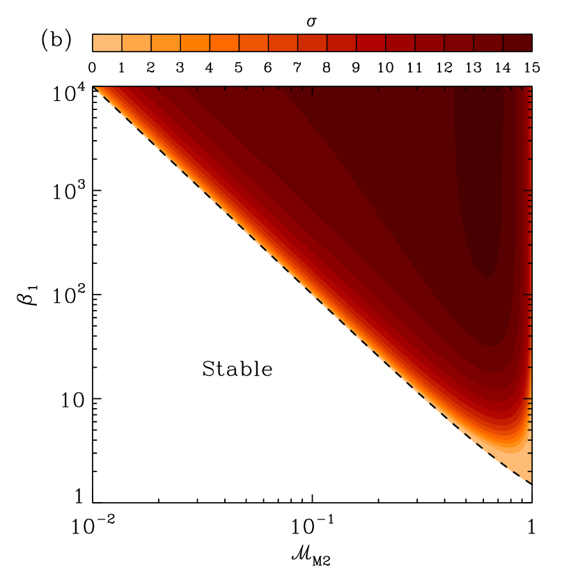
Figure 6: (a) Compressible growth rate $\sigma$ of the instability of magnetized IFs as a function of $\mathcal{M}_{\rm{M}2}$ and (b) the contour of $\sigma$ in the $\beta_{1}$-$\mathcal{M}_{\rm{M}2}$ plane. The perturbations are limited to $k_{y}=0$, and $\theta=200$ and $G=0$ are chosen. The instability is suppressed by magnetic tension at low $\mathcal{M}_{\rm{M}2}$ and by compressibility at $\mathcal{M}_{\rm{M}2}\rightarrow 1$. The black dashed line in (b) draws the stability criteria (Equation (111)) in the limit $\theta\gg 1$, in good agreement with the full numerical results.

6 Summary and Discussion

6.1 Summary

We have performed a linear stability analysis of magnetized, weak D-type IFs around H II regions. This work extends Vandervoort (1962) who analyzed the stability of IFs in the absence of magnetic fields. To simplify the situation, we consider an IF in plane-parallel geometry, perpendicular to the incident direction of ionizing photons, and ignore the effects of recombination in the ionized gas in the present work. We further assume that magnetic fields are parallel to the front and that the gas remains isothermal with different temperatures in the neutral and ionized sides of the front. We first solve for equilibrium configurations of steady IFs across which total mass, momentum, and magnetic fluxes are conserved. We find that for weak D-type IFs, magnetic fields tend to increase the maximum propagation speed of the IFs, while reducing the expansion factor $\alpha$ by a factor of $1+1/(2\beta_{1})$ compared to the unmagnetized case (see Equations (29) and (30)). In the stationary IF frame, the magnetosonic Mach number of the ionized gas downstream from the IF always satisfies $\mathcal{M}_{\rm{M}2}^{2}\leq 1$ for weak D-type fronts, with the equality corresponding to the D-critical fronts. We provide the approximate expressions (Equations (27) and (28)) for the expansion factors and sonic Mach numbers when the fronts are either D- or R-critical.

We impose small-amplitude perturbations on a steady-state IF in isolation, and seek for unstable modes that grow exponentially in time. The perturbations are constructed as a superposition of MHD waves that are evanescent far away from the IF; only the fast (or acoustic) mode propagates in the upstream side, while both fast and slow (or vortex) modes exist in the downstream side for an isolated magnetized (or unmagnetized) front. For the two-dimensional perturbations we impose, shear Alfvén waves are not excited. We require that the perturbation variables satisfy the perturbed jump conditions (Equations (72)–(78)) at the IF to derive the dispersion relations of the instability.

We first apply our technique to unmagnetized IFs. The resulting dispersion relation (Equation (86)) recovers the result of Vandervoort (1962). When the external gravity is ignored (i.e., $G=0$), it is also identical to the dispersion relation of the DLI seen in laser ablation fronts in inertial confinement fusion (e.g., Bychkov et al., 2008; Modestov et al., 2009). This suggests that the physical mechanism behind the IF instability is the same as that of the DLI. The DLI is generic for any interfacial layer through which a cold dense gas absorbs heat and expands to turn to a warm rarefied gas. The DLI is multi-dimensional, requiring wavy deformation of the interface in the direction normal to the incident ionizing radiation. In the case of IFs, the front deformation grows due to mismatches between the perturbed mass flux and the ionization rate of the cold gas at the IF. This is in contrast to the claim of Vandervoort (1962) that the IF instability is due to the rocket effect (Kahn, 1954; Oort & Spitzer, 1955) which, unlike the DLI, does not require wavy deformation of the IF, and relies on high-speed evaporating gas from a dense cloud to exert thrust on it.

The unstable mode of the IF instability grows without oscillation, indicative of pure instability. The growth rate scales linearly with the wavenumber as well as the background fluid velocity relative to the front. The dimensionless growth rate increases with $\alpha^{1/2}$ for $\alpha\gg 1$ (Equation (89)). As $\mathcal{M}_{\rm{S2}}$ increases, the instability is stabilized by gas compressibility which tends to reduce the change in mass flux at the IF, becoming completely quenched when the front is D-critical ($\mathcal{M}_{\rm{S2}}=1$). The IF instability cooperates with the RTI for IFs accelerating away from an ionizing source ($G>0$), while it is suppressed by buoyancy for decelerating IFs at large scales (Equation (90)).

For magnetized fronts, we consider two cases of two-dimensional perturbations: (1) perturbations with $k_{x}=0$ are in the plane perpendicular to the magnetic fields and (2) perturbations with $k_{y}=0$ are confined to the plane defined by the magnetic fields and the background flows. For the $k_{x}=0$ perturbations, the perturbed fields exert only magnetic pressure forces and the resulting dispersion relation is identical to the hydrodynamic case, provided the sound speed is replaced by the speed of magnetosonic waves. For the $k_{y}=0$ perturbations, on the other hand, magnetic tension from the bent field lines stabilizes the instability. In the incompressible limit, the dispersion relation (Equation (105)) of the IF instability is again the same as that of the DLI studied by Dursi (2004). The IF instability is completely suppressed if the Alfvénic Mach number is sufficiently small (Equation (111)), suggesting that no instability is expected if the plasma parameter $\beta_{1}$ is less than 3/2 in the upstream neutral region.

6.2 Discussion

Observations indicate that IFs are usually magnetized. Using the Zeeman effects of H I and OH lines, for instance, Brogan et al. (1999) and Brogan & Troland (2001) reported that the strength of line-of-sight magnetic fields toward the interface of H II region/molecular cloud complex in M17 is on average $\sim 200$–$500\,\mu$G and reaches a value as high as $\sim 750\,\mu$G. Taking $B_{1}\sim 300\,\mu{\rm G}$, corresponding to the magnetic pressure support of $2.6\times 10^{7}k_{\rm{B}}\,{\rm cm^{-3}\,K}$, and assuming $T_{1}=100\;{\rm K}$, $\beta_{1}$ is less than 1.5 unless $n_{1}\lower 2.15277pt\hbox{$\;\buildrel>\over{\sim}\;$}8\times 10^{5}\;\rm{cm}^{-3}$. This large background density is highly unlikely since the equilibrium model of Pellegrini et al. (2007) favors $n_{1}$ of order of $\sim 10^{4}\,{\rm cm^{-3}}$. This suggests that the IF instability is readily stabilized by magnetic tension in the direction parallel to the fields. However, the IFs in M17 can still be unstable to perturbations (with $k_{x}=0$ and $k_{y}\neq 0$) propagating in the direction perpendicular to the fields. The growth rate $\Omega=k_{y}v_{z1}\sigma$ in dimensional units can be written as

$$\Omega\approx 6.4\times 10^{-5}\frac{\mathcal{M}_{\rm{M}1}\sigma}{(1+\beta_{1}^{-1})^{1/2}}\left(\dfrac{\lambda}{0.1\;{\rm pc}}\right)\left(\dfrac{c_{\rm s1}}{1\;{\rm km\,s}^{-1}}\right)\;{\rm yr^{-1}}\,,$$ (112)

where $\lambda$ is the perturbation wavelength. For $G=0$ and $\theta=200$, the maximum value of $\mathcal{M}_{\rm{M}1}\sigma$ is $(0.19,0.3,0.40)$ for $\beta_{1}=(0.01,0.1,1)$, which occurs at $\mathcal{M}_{\rm{M}2}=0.75$ (see Figures 2(a) and 4). The corresponding $e$-folding growth time of the instability is $(2.8,1.5,0.8)\times 10^{4}\,{\rm yr}$ for $\beta_{1}=(0.01,0.1,1)$, respectively, which is an order of magnitude shorter than the typical expansion time scale of H II regions (typically $10^{5}\text{--}10^{6}\,{\rm yr}$; see below). This indicates that the IF instability with $k_{y}\neq 0$ can grow significantly, but by keeping the magnetic field lines straight.

The relative importance of the front acceleration/deceleration to the the gas kinetic energy is measured by the dimensionless parameter $G=g/(kv_{z1}^{2})$. Recently, Ricotti (2014) investigated the stabilizing effect of recombination on the RTI of accelerating IFs assuming that gas is incompressible. Due to the incompressibility assumption, however, his results (Equations (40) and (41) of (Ricotti, 2014)) in the absence of recombination recovers the dispersion relation only for the RTI, but is unable to capture the IF instability of Vandervoort (1962). A simple comparison between the growth rates of the IF instability ($\sim\sqrt{\alpha}v_{z1}k_{x}$) and the RTI ($\sim\sqrt{gk_{x}}$) suggests that the perturbed flows are strongly affected by buoyancy for $|G|\lower 2.15277pt\hbox{$\;\buildrel>\over{\sim}\;$}\alpha$. In a uniform medium without magnetic fields, Spitzer (1978) showed that a D-type IF expands as $r_{\rm IF}\approx r_{s}(1+7t/4t_{s})^{4/7}$, where $r_{s}=3.2\,{\rm pc}(Q/10^{49}\,{\rm s^{-1}})(\rho_{2}/(100\,m_{\rm{H}}\;\rm{cm}^{-3}))^{-2/3}$ is the initial Strömgren radius, $Q$ is the ionizing photon luminosity of a central star, and $t_{s}=r_{s}/c_{\rm s2}=0.24\,{\rm Myr}$ for $c_{\rm s2}=13\,{\rm km\,s^{-1}}$. The effective gravity is then $g=-3c_{\rm s2}/(4t_{s})(1+4t/7t_{s})^{-10/7}$. Taking $\theta=200$, $g=-3c_{\rm s2}/4t_{s}$, and $\mathcal{M}_{\rm{M}2}=0.5$, the IF instability is stabilized by buoyancy for perturbations with wavelength $\lambda/r_{s}>8\pi\mathcal{M}_{\rm{S2}}^{2}/(3\alpha)\sim 10^{-2}$ even for purely hydrodynamic IFs. On the other hand, for IFs accelerating outward in a stratified medium with density decreasing more steeply than $r^{-3/2}$ (e.g., Franco et al., 1990; Whalen & Norman, 2008), the RTI would work together with the IF instability to make the fronts more unstable.

We have not considered thermal conduction in our analysis since its effect on the IF instability is thought to be insignificant. This can be seen quantitatively as follows. Let us take typical values for the mean photoionization cross section $\sigma_{\rm{ph}}=3\times 10^{-18}\;\rm{cm}^{2}$, the mean kinetic energy of a photo-ejected electron $\langle E_{\rm ph}\rangle=2.4\;{\rm eV}$ (e.g., Whalen et al., 2004), and the incident ionizing photon flux $F_{\rm ph}=\rho_{2}v_{z2}/m_{\rm{H}}$. Then, the volumetric heating rate by photoionization amounts to $\mathcal{H}=(\rho_{2}/m_{\rm{H}})\sigma_{\rm{ph}}F_{\rm ph}\langle E_{\rm ph}\rangle=1.5\times 10^{-19}(\rho_{2}/(100\,m_{\rm{H}}\;\rm{cm}^{-3}))(c_{\rm s2}/13\,{\rm km\,s^{-1}})\mathcal{M}_{\rm{S2}}\;{\rm erg}\,{\rm cm}^{-3}\,{\rm s}^{-1}$. For the Spitzer conductivity of $\kappa_{\rm Sp}\sim 10^{4}\;{\rm erg}\,{\rm cm}^{-1}\,{\rm s}^{-1}\,{\rm K}^{-1}$ in the ionized gas with $T_{2}=10^{4}\;{\rm K}$ (McKee & Cowie, 1977), the Field length is calculated to be $L_{\rm{F2}}=\sqrt{\kappa_{\rm Sp}T_{2}/\mathcal{H}}=8.4\times 10^{-6}\;\rm{pc}$, while the thermal diffusion length is $L_{\rm{D2}}=\kappa_{2}/(j_{z}c_{P})=2\times 10^{-5}\;\rm{pc}$, where $c_{P}$ is the specific heat at constant pressure (e.g., Kim & Kim 2013). Note that the photon mean-free path $L_{\rm{mfp2}}=1/(n_{2}\sigma_{\rm{ph}})=10^{-3}\;\rm{pc}$ is much larger than the conduction length scales. Therefore, thermal diffusion is unlikely to be important in determining the structures of IFs as well as the IF instability (see also Spitzer 1978). This is in contrast to the case of evaporation fronts between cold and warm gases studied by Kim & Kim (2013), where thermal conduction not only affects the front thickness but also stabilizes the DLI at small scales.

Can the IF instability manifest in numerical simulations of expanding H II regions? In Eulerian simulations, it is unavoidable to have spurious numerical viscosity, caused by a finite difference scheme, that dampens perturbations at small scale. Kim et al. (2008) found that the numerical diffusivity can be written as $\eta=A_{d}v_{\rm ad}\Delta x(\Delta x/\lambda)^{n}$, where $A_{d}$ is a dimensionless constant, $\lambda$ is the characteristic length scale of perturbations, $\Delta x$ is the grid spacing, $v_{\rm ad}$ is the advection velocity through a numerical grid, and $n$ is the order of the spatial reconstruction in the numerical scheme. Since the corresponding damping time over the scale of $\lambda$ is $\tau_{\eta}\sim\lambda^{2}/\eta$, the numerical diffusion would prohibit the growth of the IF instability if $\tau_{\eta}\Omega\lesssim 1$ or if $\lambda/\Delta x\lesssim(A_{d}\alpha v_{\rm ad}/2\pi v_{z2}\sigma)^{1/(n+1)}$. Taking $A_{d}=8.1\times 10^{4}$ and $n=2$ from Kim & Stone (2012) for the Athena code with piecewise-linear reconstruction scheme, for example, and taking $\alpha/\sigma\sim 10$ and $v_{\rm ad}/v_{z2}=1$, one can see that perturbations with $\lambda/\Delta x\gtrsim 50$ would be stabilized by numerical effects. Considering the typical resolution of $\Delta x\sim 10^{-2}\text{--}10^{-1}\,\;\rm{pc}$ in simulations of a single H II region (e.g., Krumholz et al., 2007; Mackey & Lim, 2011; Arthur et al., 2011), the DLI mode below $\sim 0.1$–$1\,\rm{pc}$ would be suppressed by numerical diffusion. Modes with wavelength longer than these may still grow, but too slowly to be readily evident in numerical simulations. Therefore, very high-resolution simulations are desirable to resolve the IF instability at small scales.

Finally, we remark a few caveats made by our simplified model of an IF. First, the approximation of stationary IFs in plane-parallel geometry ignores the curvature effect as well as temporal changes in the background state, while IFs in reality have non-vanishing curvature, especially in the case of ablated globules. As an IF propagates, its curvature and the Mach number of the inflowing neutral gas would vary. For an expanding H II region, the perturbation wavelength increases in proportion to the size of the H II region, resulting in a power-law growth rather than an exponential growth (Zeldovich et al., 1985). Second, IFs associated with blister-type H II regions and cometary globules (e.g., Kahn 1969; Bertoldi 1989; Bertoldi & McKee 1990) are strong D-type (or D-critical) and the ionized gas accelerates away from such IFs to achieve a supersonic speed. With spatially-varying density and velocity fields in the background state, instability of strong D-type IFs cannot be explored by our current technique that assumes uniform backgrounds in the upstream and downstream sides. Third, a D-type IF is usually preceded by a shock front, indicating that some waves launched by the IF would undergo reflection at the shock front, which is likely to alter the modal behavior of the perturbations in the upstream side. It is well known that after a shock breakout, the shocked layer is subject to a thin-shell instability due to the force imbalance between thermal and ram pressures at the boundaries (Giuliani, 1979; Vishniac, 1983; Garcia-Segura & Franco, 1996). Right after the shock breakout (i.e., when the fronts are near D-critical), the gas ahead of the IF is subject to significant non-steady cooling and heating, so that the isothermal approximation in the neutral gas may not be applicable (Henney et al., 2009). In this case, a proper account of radiative cooling/heating is necessary to assess the impact of nonlinear development of the IF instability (Whalen & Norman, 2008).

Appendix A Derivation of Equation (76)

Here we present steps to derive Equation (76). Using Equations (72) and (73), Equation (67) is reduced to

$$(1-\mathcal{M}_{\rm{S1}}^{2})p_{1}^{\prime}+\mathcal{M}_{\rm{A1}}^{-1}b_{x1}^{\prime}-\mathcal{M}_{\rm{A2}}^{-1}b_{x2}^{\prime}+(1-\alpha^{-1})GZ=(1-\mathcal{M}_{\rm{S1}}^{2})p_{2}^{\prime}\,.$$ (A1)

Combining Equations (77) and (A1), one may write

$$(1+\beta_{1}^{-1}-\mathcal{M}_{\rm{S1}}^{2})p_{1}^{\prime}+(1-\alpha^{-2})(\mathcal{M}_{\rm{A1}}^{-1}b_{x1}^{\prime}-\beta_{1}^{-1}p_{1}^{\prime})+(1-\alpha^{-1})GZ=(1+\beta_{2}^{-1}-\mathcal{M}_{\rm{S2}}^{2})p_{2}^{\prime}\,.$$ (A2)

As we shall show in Sections 4 and 5, the perturbations in the upstream side (region 1) are described only by fast modes that obey Equations (47)–(49). Hence, one can write for fast modes

$$\mathcal{M}_{\rm{A1}}^{-1}b_{x1}^{\prime}-\beta_{1}^{-1}p_{1}^{\prime} =\left(\dfrac{\mathcal{M}_{\rm{A1}}^{-2}(\nu^{2}-\sin^{2}\psi)}{\chi}-\frac{1}{\beta_{1}}\right)p_{1}^{\prime}\,,$$ (A3)

$$=\cos^{2}\psi\dfrac{\mathcal{M}_{\rm{A1}}^{-2}}{(\sigma+\nu)^{2}}p_{1}^{\prime}\,,$$ (A4)

where $\chi=\sigma_{D}^{2}+\hat{\alpha}^{2}\mathcal{M}_{\rm{A}}^{-2}(1-\nu^{2})$ and we have used Equation (53) in the last equality. Combining Equations (A2) and (A4) gives Equation (76).

Appendix B Perturbation Equations for $k_{x}\neq 0$ and $k_{y}=0$

We plug Equations (109) and (110) into Equations (72)–(74) and (76)–(77), and arrange terms to obtain

$$\mathbf{A}\cdot(C_{\rm f1},C_{\rm f2},C_{\rm s2+},C_{\rm s2-},Z)^{T}=0\,,$$ (B1)

where $\mathbf{A}$ is a $5\times 5$ matrix whose components are given by

$$\begin{split}A_{11}&=1-\mathcal{M}_{\rm{S1}}^{2}\chi_{\rm f1}/(\nu_{\rm f1}\sigma_{D,{\rm f1}})\,,\\ A_{1j}&=0\,,\\ A_{15}&=-\sigma\,,\\ \end{split}$$ (B2)

$$\begin{split}A_{21}&=0\,,\\ A_{2j}&=1-\mathcal{M}_{\rm{S2}}^{2}\chi_{j}/(\alpha\nu_{j}\sigma_{D,j})\,,\\ A_{25}&=-\sigma\,,\end{split}$$ (B3)

$$\begin{split}A_{31}&=\chi_{\rm f1}/(\nu_{\rm f1}\sigma_{D,{\rm f1}}^{2})-\mathcal{M}_{\rm{A1}}^{-2}/\sigma_{D,{\rm f1}}\,,\\ A_{3j}&=\chi_{j}/(\nu_{j}\sigma_{D,j}^{2})-\alpha\mathcal{M}_{\rm{A2}}^{-2}/\sigma_{D,j}\,,\\ A_{35}&=1+\mathcal{M}_{\rm{A1}}^{-2}-\alpha(1+\mathcal{M}_{\rm{A2}}^{-2})\,,\end{split}$$ (B4)

$$\begin{split}A_{41}&=-\mathcal{B}\chi_{\rm f1}/(\nu_{\rm f1}\sigma_{D,{\rm f1}})\,,\\ A_{4j}&=(1+\beta_{2}^{-1})(1-\mathcal{M}_{\rm{M}2}^{2})\chi_{j}/(\alpha\nu_{j}\sigma_{D,j})\,,\\ A_{45}&=(1-\alpha^{-1})G\,,\end{split}$$ (B5)

$$\begin{split}A_{51}&=-\nu_{\rm f1}\mathcal{M}_{\rm{A1}}^{-1}/\sigma_{D,{\rm f1}}+\mathcal{M}_{\rm{A1}}^{-1}\mathcal{M}_{\rm{S1}}^{2}\chi_{\rm f1}/(\nu_{\rm f1}\sigma_{D,{\rm f1}})\,,\\ A_{5j}&=\alpha^{3/2}\mathcal{M}_{\rm{A2}}^{-1}\nu_{j}/\sigma_{D,j}-\mathcal{M}_{\rm{A2}}^{-1}\mathcal{M}_{\rm{S2}}^{2}\chi_{j}/(\alpha^{1/2}\nu_{j}\sigma_{D,j})\,,\\ A_{55}&=0\,.\end{split}$$ (B6)

Here,

$$\mathcal{B}=(1+\beta_{1}^{-1})(1-\mathcal{M}_{\rm{M}1}^{2})+\dfrac{\mathcal{M}_{\rm{A1}}^{-2}(1-\alpha^{-2})}{(\sigma+\nu_{\rm f1})^{2}}\,,$$ (B7)

and the index $j$ in Equations (B3)–(B6) runs from 2 to 4, with $j=2$, 3, and 4 corresponding to the downstream fast ($\rm{f2}$), forward-propagating slow ($\rm{s2+}$), and backward-propagating slow ($\rm{s2-}$) modes, respectively.

References

- Arthur et al. (2011) Arthur, S. J., Henney, W. J., Mellema, G., de Colle, F., & Vázquez-Semadeni, E. 2011, MNRAS, 414, 1747
- Axford (1961) Axford, W. I. 1961, RSPTA, 253, 301
- Axford (1964) —. 1964, ApJ, 140, 112
- Bell et al. (2004) Bell, J. B., Day, M. S., Rendleman, C. A., Woosley, S. E., & Zingale, M. 2004, ApJ, 606, 1029
- Bertoldi (1989) Bertoldi, F. 1989, ApJ, 346, 735
- Bertoldi & McKee (1990) Bertoldi, F., & McKee, C. F. 1990. ApJ, 354, 529
- Bisbas et al. (2011) Bisbas, T. G., Wünsch, R., Whitworth, A. P., Hubber, D. A., & Walch, S. 2011, ApJ, 736, 142
- Brogan & Troland (2001) Brogan, C. L., & Troland, T. H. 2001, ApJ, 560, 821
- Brogan et al. (2005) Brogan, C. L., Troland, T. H., Abel, N. P., Goss, W. M., & Crutcher, R. M. 2005, in Astronomical Society of the Pacific Conference Series, Vol. 343, Astronomical Polarimetry: Current Status and Future Directions, ed. A. Adamson, C. Aspin, C. Davis, & T. Fujiyoshi, 183
- Brogan et al. (1999) Brogan, C. L., Troland, T. H., Roberts, D. A., & Crutcher, R. M. 1999, ApJ, 515, 304
- Bychkov et al. (1994) Bychkov, V. V., Golberg, S. M., & Liberman, M. A., 1994, PhPl, 1, 2976
- Bychkov et al. (2008) Bychkov, V., Modestov, M., & Marklund, M. 2008, PhPl, 15, 032702
- Chandrasekhar (1961) Chandrasekhar, S. 1961, Hydrodynamic and hydromagnetic stability (Oxford: Dover)
- Churchwell et al. (2006) Churchwell, E., et al. 2006, ApJ, 649, 759
- Crutcher (1999) Crutcher, R. M. 1999, ApJ, 520, 706
- Dale et al. (2012) Dale, J. E., Ercolano, B., & Bonnell, I. A. 2012, MNRAS, 424, 377
- Dale et al. (2009) Dale, J. E., Wünsch, R., Whitworth, A., & Palouš, J. 2009, MNRAS, 398, 1537
- Draine (2011) Draine, B. T. 2011, Physics of the Interstellar and Intergalactic Medium, Princeton Series in Astrophysics (Princeton, NJ: Princeton Univ. Press)
- Dursi (2004) Dursi, L. J. 2004, ApJ, 606, 1039
- Elmegreen & Lada (1977) Elmegreen, B. G., & Lada, C. J. 1977, ApJ, 214, 725
- Franco et al. (1990) Franco, J., Tenorio-Tagle, G., & Bodenheimer, P. 1990, ApJ, 349, 126
- Frieman (1954) Frieman, E. A. 1954, ApJ, 120, 18
- Garcia-Segura & Franco (1996) Garcia-Segura, G., & Franco, J. 1996, ApJ, 469, 171
- Giuliani (1979) Giuliani, Jr., J. L. 1979, ApJ, 233, 280
- Goldsworthy (1958) Goldsworthy, F. A. 1958, RvMP, 30, 1062
- Gritschneder et al. (2010) Gritschneder, M., Burkert, A., Naab, T., & Walch, S. 2010, ApJ, 723, 971
- Harvey-Smith et al. (2011) Harvey-Smith, L., Madsen, G. J., & Gaensler, B. M. 2011, ApJ, 736, 83
- Heiles & Chu (1980) Heiles, C., & Chu, Y.-H. 1980, ApJ, 235, L105
- Heiles et al. (1981) Heiles, C., Chu, Y.-H., & Troland, T. H. 1981, ApJ, 247, L77
- Heiles & Crutcher (2005) Heiles, C., & Crutcher, R. 2005, in Lecture Notes in Physics, Berlin Springer Verlag, Vol. 664, Cosmic Magnetic Fields, ed. R. Wielebinski & R. Beck, 137
- Henney et al. (2009) Henney, W. J., Arthur, S. J., de Colle, F., & Mellema, G. 2009, MNRAS, 398, 157
- Hester et al. (1996) Hester, J. J., et al. 1996, AJ, 111, 2349
- Hosokawa & Inutsuka (2006) Hosokawa, T., & Inutsuka, S.-i. 2006, ApJ, 646, 240
- Inoue et al. (2006) Inoue, T., Inutsuka, S.-i., & Koyama, H. 2006, ApJ, 652, 1331
- Iwasaki et al. (2011) Iwasaki, K., Inutsuka, S.-i., & Tsuribe, T. 2011, ApJ, 733, 17
- Kahn (1954) Kahn, F. D. 1954, BAN, 12, 187
- Kahn (1969) Kahn, F. D. 1969, Phy, 41, 172
- Kim et al. (2008) Kim, C.-G., Kim, W.-T., & Ostriker, E. C. 2008, ApJ, 681, 1148
- Kim & Kim (2013) Kim, J.-G., & Kim, W.-T. 2013, ApJ, 779, 48
- Kim & Stone (2012) Kim, W.-T., & Stone, J. M. 2012, ApJ, 751, 124
- Krumholz et al. (2006) Krumholz, M. R., Matzner, C. D., & McKee, C. F. 2006, ApJ, 653, 361
- Krumholz et al. (2007) Krumholz, M. R., Stone, J. M., & Gardiner, T. A. 2007, ApJ, 671, 518
- Krumholz et al. (2014) Krumholz, M. R., Bate, M. R., Arce, H. G., et al. 2014, to appear in Protostars and Planets VI, eds. H. Beuther, R. Klessen, C. Dullemond, & Th. Henning (Univ. of Arizona Press); arXiv:1401.2473
- Landau & Lifshitz (1959) Landau, L. D., & Lifshitz, E. M. 1959, Fluid mechanics (New York: Pergamon)
- Lasker (1966) Lasker, B. M. 1966, ApJ, 146, 471
- Lithwick & Goldreich (2001) Lithwick, Y., & Goldreich, P. 2001, ApJ, 562, 279
- Mackey & Lim (2011) Mackey, J., & Lim, A. J. 2011, MNRAS, 412, 2079
- Mathews (1965) Mathews, W. G. 1965, ApJ, 142, 1120
- Matzner (2002) Matzner, C. D. 2002, ApJ, 566, 302
- McKee & Cowie (1977) McKee, C. F., & Cowie, L. L. 1977, ApJ, 215, 213
- Mellema et al. (2006) Mellema, G., Arthur, S. J., Henney, W. J., Iliev, I. T., & Shapiro, P. R. 2006, ApJ, 647, 397
- Mizuta et al. (2005) Mizuta, A., Kane, J. O., Pound, M. W., Remington, B. A., Ryutov, D. D., & Takabe, H. 2005, ApJ, 621, 803
- Modestov et al. (2009) Modestov, M., Bychkov, V., Valiev, D., & Marklund, M. 2009, PhRvE, 80, 046403
- Oort & Spitzer (1955) Oort, J. H., & Spitzer, Jr., L. 1955, ApJ, 121, 6
- Park et al. (2014) Park, K., Ricotti, M., Di Matteo, T., & Reynolds, C. S. 2014, MNRAS, 437, 2856
- Pellegrini et al. (2009) Pellegrini, E. W., Baldwin, J. A., Ferland, G. J., Shaw, G., & Heathcote, S. 2009, ApJ, 693, 285
- Pellegrini et al. (2007) Pellegrini, E. W., et al. 2007, ApJ, 658, 1119
- Redman et al. (1998) Redman, M. P., Williams, R. J. R., Dyson, J. E., Hartquist, T. W., & Fernandez, B. R. 1998, A&A, 331, 1099
- Ricotti (2014) Ricotti, M. 2014, MNRAS, 437, 371
- Rodríguez et al. (2012) Rodríguez, L. F., Gómez, Y., & Tafoya, D. 2012, MNRAS, 420, 279
- Saaf (1966) Saaf, A. F. 1966, ApJ, 145, 116
- Sandford et al. (1982) Sandford, II, M. T., Whitaker, R. W., & Klein, R. I. 1982, ApJ, 260, 183
- Shu (1992) Shu, F. H. 1992, The Physics of Astrophysics. Volume II: Gas Dynamics., ed. F. H. Shu (Mill Valley, CA: Univ. Science Books)
- Spitzer (1954) Spitzer, Jr., L. 1954, ApJ, 120, 1
- Spitzer (1978) —. 1978, Physical processes in the interstellar medium (New York: Academic Press)
- Stone & Zweibel (2009) Stone, J. M., & Zweibel, E. G. 2009, ApJ, 696, 233
- Strömgren (1939) Strömgren, B. 1939, ApJ, 89, 526
- Sugitani et al. (1991) Sugitani, K., Fukui, Y., & Ogura, K. 1991, ApJS, 77, 59
- Sysoev (1997) Sysoev, N. E. 1997, AstL, 23, 409
- Takabe et al. (1985) Takabe, H., Mima, K., Montierth, L., & Morse, R. L. 1985, PhFl, 28, 3676
- Tremblin et al. (2012a) Tremblin, P., Audit, E., Minier, V., Schmidt, W., & Schneider, N. 2012a, A&A, 546, A33
- Tremblin et al. (2012b) —. 2012b, A&A, 546, A33
- Vandervoort (1962) Vandervoort, P. O. 1962, ApJ, 135, 212
- Vishniac (1983) Vishniac, E. T. 1983, ApJ, 274, 152
- Walch et al. (2012) Walch, S. K., Whitworth, A. P., Bisbas, T., Wünsch, R., & Hubber, D. 2012, MNRAS, 427, 625
- Whalen et al. (2004) Whalen, D., Abel, T., & Norman, M. L. 2004, ApJ, 610, 14
- Whalen & Norman (2008) Whalen, D. J., & Norman, M. L. 2008, ApJ, 672, 287
- Williams (2002) Williams, R. J. R. 2002, MNRAS, 331, 693
- Williams et al. (2000) Williams, R. J. R., Dyson, J. E., & Hartquist, T. W. 2000, MNRAS, 314, 315
- Yorke (1986) Yorke, H. W. 1986, ARA&A, 24, 49
- Zeldovich et al. (1985) Zeldovich, Y. B., Barenblatt, G. I., Librovich, V. B., & Makhviladze, G. M. 1985, The Mathematical Theory of Combustion and Explosions (Consultants Bureau)