Flavour violating lepton decays in low-scale seesaws

Abstract

We present the first complete calculation of flavour violating lepton decays taking into account all supersymmetric (SUSY) and non-SUSY contributions in the context of the supersymmetric inverse seesaw, a specific SUSY low-scale seesaw model. We consider radiative and 3-body lepton decays as well as neutrinoless $\mu-e$ conversion in muonic atoms and perform a full one-loop calculation in the mass basis. Taking CMSSM-like boundary conditions for the soft SUSY breaking parameters, we find that cancellations between different contributions are present in several regions, which might reduce the branching ratios by as much as one order of magnitude. This has important consequences when translating current measurements into constraints and estimating the reach of future experiments, and justifies the use of a full calculation. We also show that the ratio of different cross-sections can discriminate between dominant SUSY or non-SUSY contributions.

1 Introduction

Since their experimental confirmation two decades ago, neutrino oscillations have been extensively studied and all but two parameters have been precisely measured: the neutrinos mass ordering and a CP violating phase [1]. This observation constitutes the only signal of new physics observed so far that absolutely calls for an extension of the Standard Model (SM). A simple and attractive possibility to generate neutrino masses and mixing is the Inverse Seesaw (ISS) mechanism [2, 3, 4]. It extends the SM by adding pairs of fermionic singlets with a seesaw scale close to the electroweak scale and naturally large neutrino Yukawa couplings. However, the SM suffers from other theoretical and observational issues like the absence of a dark matter candidate or the hierarchy problem. Supersymmetry (SUSY) naturally solves these problems and the supersymmetric inverse seesaw model addresses all these issues in a common framework where all the new physics is located around the TeV scale.

While many neutrino mass generating mechanisms lead to the same phenomenology when it comes to neutrino oscillations, they can be distinguished by searching for the effects of the new particles that they introduce. Those effects can be modified decay chains at high-energy colliders due to the production of the new particles or indirect effects in low-energy experiments. Charged lepton flavour violating (cLFV) processes are particularly attractive since they are free from Standard Model background and their cross-sections strongly depend on the model considered. Besides, there is an intense experimental effort in this field and huge sensitivity improvements are expected in the future, up to five orders of magnitude for neutrinoless $\mu-e$ conversion for example [5, 6]. In this work, we focus on cLFV radiative and 3-body lepton decays as well as neutrinoless $\mu-e$ conversion in muonic atoms. Further details, including all formulas, can be found in [7, 8].

2 The supersymmetric inverse seesaw model

The supersymmetric inverse seesaw consists of the MSSM extended by three pairs of gauge singlet superfields, $\widehat{\nu}^{c}_{i}$ and $\widehat{X}_{i}$ ($i=1,2,3$), with opposite lepton number, $-1$ and $+1$, respectively. The superpotential of this model is given by

$$W=W_{\mathrm{MSSM}}+\varepsilon_{ab}Y^{ij}_{\nu}\widehat{\nu}^{C}_{i}\widehat{L}^{a}_{j}\widehat{H}_{u}^{b}+M_{R_{ij}}\widehat{\nu}^{C}_{i}\widehat{X}_{j}+\frac{1}{2}\mu_{X_{ij}}\widehat{X}_{i}\widehat{X}_{j}\,,$$ (1)

with $W_{\mathrm{MSSM}}$ the superpotential of the MSSM. The corresponding terms of the soft SUSY breaking Lagrangian are given by

$$-\mathcal{L}^{\mathrm{soft}} =-\mathcal{L}_{\mathrm{MSSM}}^{\mathrm{soft}}+\widetilde{\nu}^{C}_{i}m^{2}_{\widetilde{\nu}^{C}_{ij}}\widetilde{\nu}^{C*}_{j}+\widetilde{X}^{*}_{i}m^{2}_{X_{ij}}\widetilde{X}_{j}$$

$$+(T_{\nu}^{ij}\varepsilon_{ab}\widetilde{\nu}^{C}_{i}\widetilde{L}^{a}_{j}H_{u}^{b}+B_{M_{R}}^{ij}\widetilde{\nu}^{C}_{i}\widetilde{X}_{j}$$

$$+\frac{1}{2}B_{\mu_{X}}^{ij}\widetilde{X}_{i}\widetilde{X}_{j}+\widetilde{X}^{*}_{i}m^{2}_{X\nu^{C}_{ij}}\widetilde{\nu}^{C}_{j}+\mathrm{h.c.})\,,$$ (2)

with $\mathcal{L}_{\mathrm{MSSM}}^{\mathrm{soft}}$ the soft SUSY breaking terms of the MSSM. The only terms that violate lepton number conservation are the Majorana mass term $\mu_{X_{ij}}\widehat{X}_{i}\widehat{X}_{j}$ and the last two terms of the soft SUSY breaking Lagrangian, $B_{\mu_{X}}^{ij}\widetilde{X}_{i}\widetilde{X}_{j}$ and $\widetilde{X}^{*}_{i}m^{2}_{X\nu^{C}_{ij}}\widetilde{\nu}^{C}_{j}$. Thus, taking them to zero increases the symmetry of the model, making their smallness natural.

After electroweak symmetry breaking, the $9\times 9$ neutrino mass matrix is given by

$$M_{\mathrm{ISS}}=\left(\begin{array}[]{c c c}0&m_{D}^{T}&0\\ m_{D}&0&M_{R}\\ 0&M_{R}^{T}&\mu_{X}\end{array}\right)\,,$$ (3)

in the basis $(\nu_{L},\,\nu_{R}^{C},\,X)$, where $m_{D}=\frac{1}{\sqrt{2}}Y_{\nu}v_{u}$ and $v_{u}/\sqrt{2}$ is the vacuum expectation value of the up-type Higgs boson. Assuming $\mu_{X}\ll m_{D}\ll M_{R}$, the neutrino mass matrix can be block-diagonalized to give the effective mass matrix for the light neutrinos [9]

$$M_{\mathrm{light}}\simeq m_{D}^{T}{M_{R}^{T}}^{-1}\mu_{X}M_{R}^{-1}m_{D}\,,$$ (4)

while the heavy neutrinos form pseudo-Dirac pairs with masses corresponding approximately to the eigenvalues of $M_{R}$. We can see from Eq. 4 that the lightness of the active neutrinos is directly related to the overall smallness of $\mu$. This decouples the smallness of the active neutrino masses from the product $M_{R}^{-1}m_{D}$ that controls the active-sterile mixing, potentially allowing for large effects in low-energy observables.

3 cLFV observables and numerical set-up

In this work, we focused on coherent neutrinoless $\mu-e$ conversion in nuclei, the cLFV radiative decays $\ell_{\alpha}\to\ell_{\beta}\gamma$ and the following 3-body decays: $\ell_{\alpha}^{-}\to\ell_{\beta}^{-}\ell_{\beta}^{-}\ell_{\beta}^{+}$, $\ell_{\alpha}^{-}\to\ell_{\beta}^{-}\ell_{\gamma}^{-}\ell_{\gamma}^{+}$ and $\ell_{\alpha}^{-}\to\ell_{\beta}^{+}\ell_{\gamma}^{-}\ell_{\gamma}^{-}$. The analytical formulas for the corresponding decay widths in terms of form factors, as well as the detailed calculation of these form factors including all possible contributions at the one-loop level in the mass basis can be found in our main article [8].　The current upper limits on the branching ratio of these processes and the expected sensitivities are given in table 1.

cLFV Process	Present Bound	Future Sensitivity
$\mu\rightarrow e\gamma$	$5.7\times 10^{-13}$ [10]	$6\times 10^{-14}$ [11]
$\tau\to e\gamma$	$3.3\times 10^{-8}$ [12]	$\sim 3\times 10^{-9}$ [13]
$\tau\to\mu\gamma$	$4.4\times 10^{-8}$ [12]	$\sim 3\times 10^{-9}$ [13]
$\mu\rightarrow eee$	$1.0\times 10^{-12}$ [14]	$\sim 10^{-16}$ [15]
$\tau\rightarrow\mu\mu\mu$	$2.1\times 10^{-8}$ [16]	$\sim 10^{-9}$ [13]
$\tau^{-}\rightarrow e^{-}\mu^{+}\mu^{-}$	$2.7\times 10^{-8}$ [16]	$\sim 10^{-9}$ [13]
$\tau^{-}\rightarrow\mu^{-}e^{+}e^{-}$	$1.8\times 10^{-8}$ [16]	$\sim 10^{-9}$ [13]
$\tau\rightarrow eee$	$2.7\times 10^{-8}$ [16]	$\sim 10^{-9}$ [13]
$\mu^{-},\mathrm{Ti}\rightarrow e^{-},\mathrm{Ti}$	$4.3\times 10^{-12}$ [17]	$\sim 10^{-18}$ [6]
$\mu^{-},\mathrm{Au}\rightarrow e^{-},\mathrm{Au}$	$7\times 10^{-13}$ [18]
$\mu^{-},\mathrm{Al}\rightarrow e^{-},\mathrm{Al}$		$10^{-15}-10^{-18}$
$\mu^{-},\mathrm{SiC}\rightarrow e^{-},\mathrm{SiC}$		$10^{-14}$ [19]

Table 1: Current experimental bounds and future sensitivities for the cLFV observables considered.

To perform our calculations and the numerical study, we have used the FlavorKit interface [20] which is a newly developed tool that allows for the easy study of flavour observables in models beyond the SM, performing an automated calculation of the form factors and their numerical evaluation. We make contact with low-energy neutrino data [1] by constructing the neutrino Yukawa coupling with a Casas-Ibarra parametrization [21] modified for the inverse seesaw [22, 23]. In our numerical study, we will keep the entries fixed to

$$Y_{\nu}=10^{-2}\cdot\begin{pmatrix}0.0956&-0.0589&0.0348\\ 0.616&0.594&-0.687\\ 0.404&1.78&1.91\end{pmatrix}\,,$$ (5)

which is possible because $\mu_{X}$ doesn’t affect our observables and can always be used to ensure the compatibility with low-energy neutrino data. We use CMSSM-like boundary conditions at $M_{GUT}$ and 2-loop RGEs that include the entire flavour structure of the model to evolve parameters between the relevant scales. The detailed procedure is described in our main article [8]. This leads to three types of contributions to cLFV at low-energy: neutrino loops, sneutrino loops and slepton loops with RGE-induced slepton mixing. Since it is possible in the ISS to simultaneously have large $\mathcal{O}(1)$ neutrino Yukawa couplings and a seesaw scale close to the electroweak scale, a large enhancement of all three types of contributions with respect the type I seesaw can be expected. In order to simplify the discussion of our numerical results, the various contributions have been divided in two categories, SUSY and non-SUSY. It is worth noting that, here, non-SUSY contributions do not simply correspond to the SM contributions but to those of a type II 2 Higgs doublet model (2HDM).

4 Numerical results

In the following, we will present our numerical results as functions of the seesaw scale, given by $M_{R}$, and the soft SUSY parameters taken to be $m_{0}=M_{1/2}=-A_{0}=M_{SUSY}$ in our plots. When they do not vary, these parameters take the standard values given in table 2.

$m_{0}$	1 TeV	$M_{1/2}$	1 TeV
$A_{0}$	-1.5 TeV	$M_{R}$	2 TeV
$B_{\mu_{X}}$	$100\,\mu_{X}$	$B_{M_{R}}$	$100\,M_{R}$
$\tan\beta$	10	sign$(\mu)$	+

Table 2: Standard values for the input parameters. $M_{R}$ and $\mu_{X}$ are taken diagonal and degenerate.

While this choice does not always lead to a mass in agreement with CMS and ATLAS measurements for the lightest CP-even Higgs boson, this does not impact the validity of our results. Indeed, Higgs-mediated contributions are subdominant for $\tan\beta=10$ and our results exhibit only a mild dependence on $A_{0}$ which could be adjusted to obtain the proper Higgs boson mass.

The first observable that we present is the decay $\mu\rightarrow e\gamma$. Its behaviour is representative of other radiative decays and it is one of the most constrained cLFV processes, with $\mathrm{Br}(\mu\rightarrow e\gamma)<5.7\times 10^{-13}$ at $90\%$ CL obtained by the MEG experiment [10] and an expected improvement in sensitivity to $6\times 10^{-14}$ after upgrade [11]. Our numerical results are shown in Fig. 1 where the grey area in Fig. 1

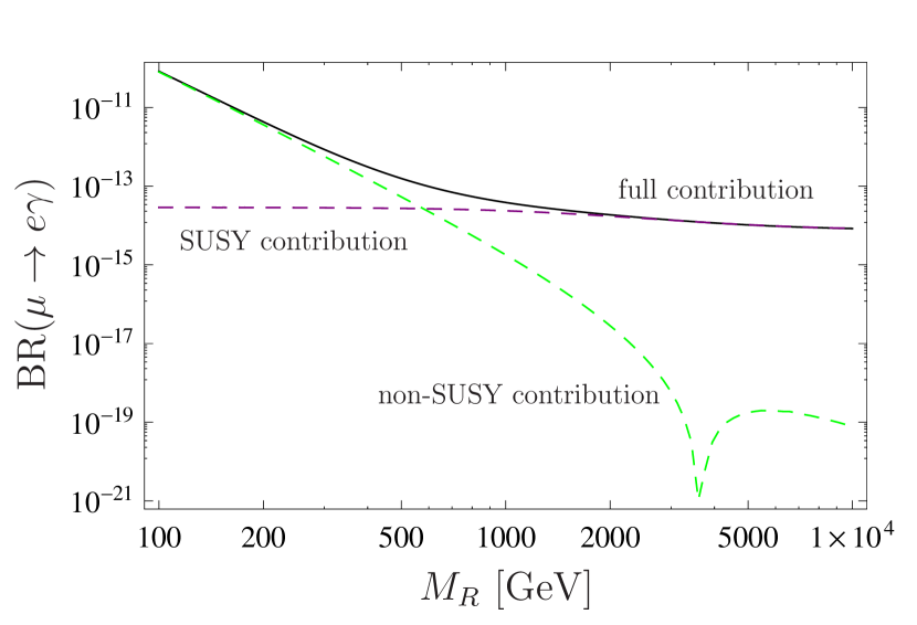
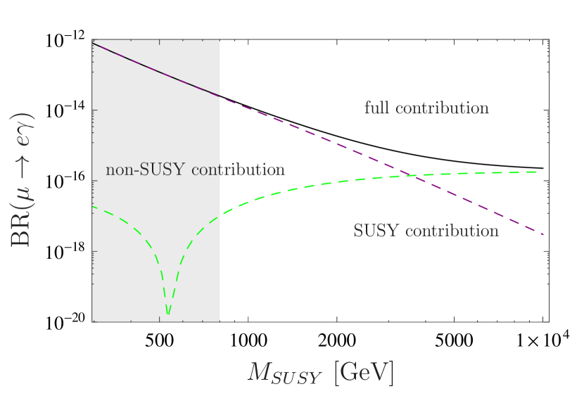
Figure 1: $\mathrm{Br}(\mu\rightarrow e\gamma)$ as a function of $M_{SUSY}$ and $M_{R}$. The grey area is excluded by the ATLAS SUSY search [24].

corresponds to the region of the CMSSM parameter space excluded by the ATLAS search [24]. We can see from both plots that our predictions saturate the current experimental limit and the dominant contribution is dictated by the lightest scale, $M_{R}$ or $M_{SUSY}$. If $M_{R}\ll M_{SUSY}$, the non-SUSY contribution dominates and vice versa. The dip in the non-SUSY contribution comes from a cancellation between $\nu-H^{\pm}$ and $\nu-W^{\pm}$ diagrams, whose matrix elements have opposite signs. The presence of this dip in Fig. 1 can be explained by the fact that scalar masses are functions of $M_{SUSY}$, explaining the dependence of non-SUSY contributions on $M_{SUSY}$. We have explicitly checked that this dependence disappears when taking the SM limit for the scalar sector.

In Fig. 2,

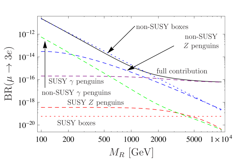
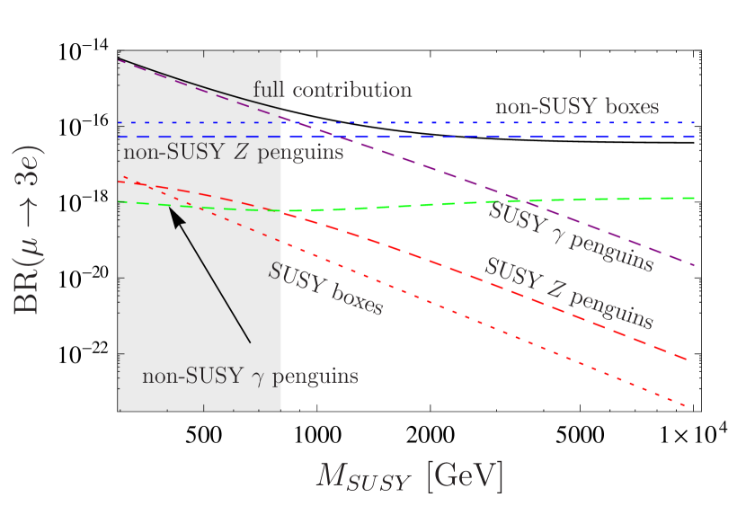
Figure 2: $\mathrm{Br}(\mu\rightarrow 3e)$ as a function of $M_{SUSY}$ and $M_{R}$. The grey area is excluded by the ATLAS SUSY search [24].

we present our results for $\mu\rightarrow 3e$. It is the cLFV 3-body decay with the lowest current experimental limit, the SINDRUM collaboration providing the upper bound $\mathrm{Br}(\mu\rightarrow 3e)<1.0\times 10^{-12}$ at $90\%$ CL [14]. While cLFV radiative decays receive contributions only from dipole operators, the phenomenology of cLFV 3-body decays is much richer with box diagrams, Z-, $\gamma$- and Higgs-penguins. The latest are not included in Fig. 2 since we found their contribution to be negligible at $\tan\beta=10$ but it would be sizeable at large $\tan\beta$ [25], typically above 50. In the case presented here, we found that the dominant SUSY contribution comes from $\gamma$-penguins, while the dominant non-SUSY contribution comes from boxes. While the latter can saturate the current experimental bound, it interferes destructively with Z-penguins, which can reduce the total branching ratio by up to one order of magnitude at large $M_{R}$. This clearly illustrates the need for a full computation and will have to be taken into account when interpreting future experimental results.

We can now turn to neutrinoless $\mu-e$ conversion in muonic atoms which similarly exhibits a rich phenomenology as can be seen from Fig. 3.

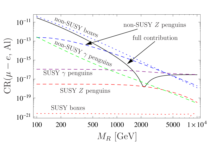
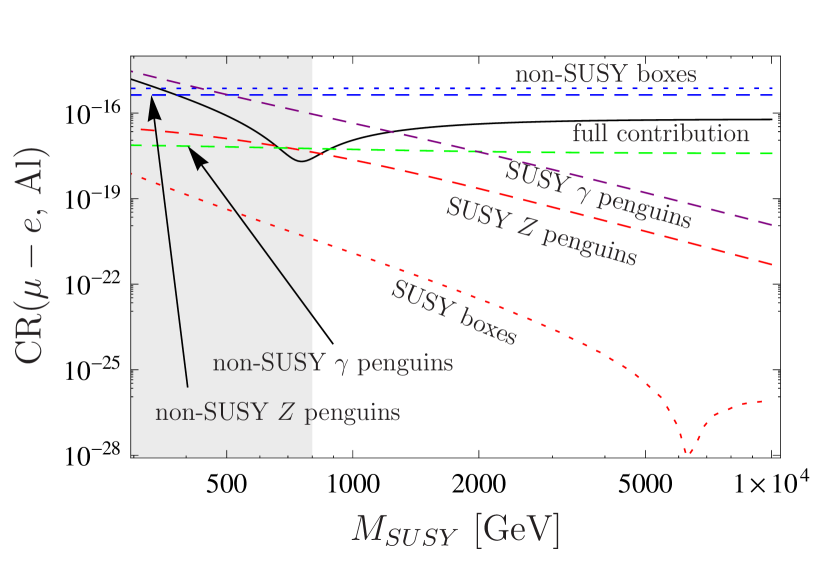
Figure 3: $\mathrm{CR}(\mu-e\,,\mathrm{Al})$ as a function of $M_{SUSY}$ and $M_{R}$. The grey area is excluded by the ATLAS SUSY search [24].

Here, the cancellation between non-SUSY boxes and Z-penguins is even more important than for $\mu\rightarrow 3e$ and, again, the dominant SUSY contribution comes from $\gamma$-penguin. Akin to $\mu\rightarrow 3e$, the conversion rate can be large enough to saturate current experimental bounds. The major difference is the appearance of a dip in the full contribution. This can easily be explained by the fact that the separate (additive) contributions for the diagrams involving quarks partially have different relative signs with respect to each other, which was not the case for those involving leptons.

Having discussed each type of cLFV observables that we considered, let us compare them with the current experimental limits and future sensitivities in mind. This can be done by plotting together the three types of observables as in Fig. 4.

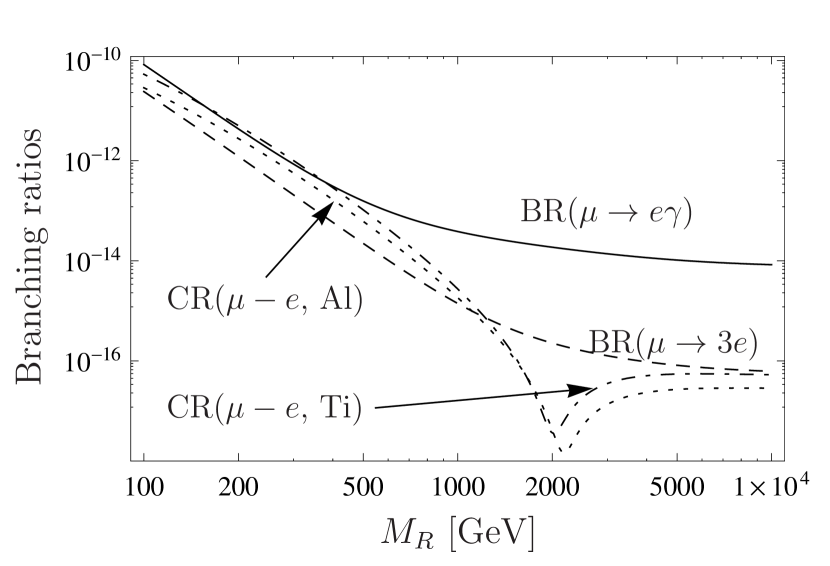
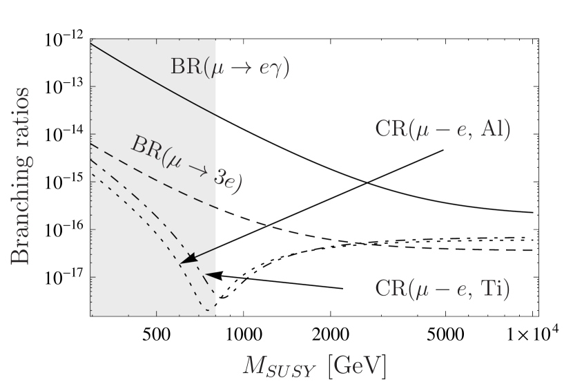
Figure 4: $\mathrm{Br}(\mu\rightarrow e\gamma)$, $\mathrm{Br}(\mu\rightarrow 3e)$, $\mathrm{CR}(\mu-e\,,\mathrm{Al})$ and $\mathrm{CR}(\mu-e\,,\mathrm{Ti})$ as functions of $M_{SUSY}$ and $M_{R}$. The grey area is excluded by the ATLAS SUSY search [24].

First, we can see that the branching ratio of $\mu\rightarrow e\gamma$ is the largest one in most of the parameter space explored. Combined with the very stringent upper limit from the MEG experiment of $5.7\times 10^{-13}$ [10], this makes $\mu\rightarrow e\gamma$ the most constraining observable in our model nowadays and in the near future. While the branching ratio of $\mu\rightarrow 3e$ is usually smaller, this observable offers the best mid-term improvement in sensitivity, the Mu3e proposal [15] mentioning a sensitivity of $\mathrm{Br}(\mu\rightarrow 3e)\sim 10^{-15}$ for the phase I in 2016 and an ultimate sensitivity of $10^{-16}$. In the long term, experiments searching for neutrinoless $\mu-e$ conversion will provide the largest improvement in sensitivity, up to five orders of magnitude and reaching sensitivities down to $10^{-18}$ around 2020. They will then be able to probe a large part of the parameter space, putting strong constraints on this model.

We have focused on $\mu$ decays up to know as they are strongly constrained and they allow to discuss the three types of cLFV observables that we have studied. We refer the interested reader to our main article [8] for results concerning $\tau$ decays. We have also discussed there the impact of the misalignment between light and heavy neutrinos as well as the effect of a non-degenerate $\mu_{X}$ matrix. There is however one last observable that would be of great interest at future B factories: the ratio of 3-body decays $\mathrm{Br}(\tau^{-}\rightarrow\ell_{\beta}^{-}\ell_{\gamma}^{+}\ell_{\gamma}^{-})/\mathrm{Br}(\tau^{-}\rightarrow 3\ell_{\beta}^{-})$. A generic prediction of the supersymmetric inverse seesaw is that $\mathrm{Br}(\tau^{-}\rightarrow\ell_{\beta}^{-}\ell_{\gamma}^{+}\ell_{\gamma}^{-})\simeq\mathrm{Br}(\tau^{-}\rightarrow 3\ell_{\beta}^{-})$. However, the exact value of their ratio is very sensitive to the dominant contribution as can be seen from Fig. 5.

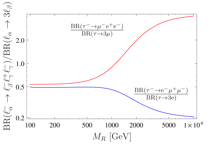
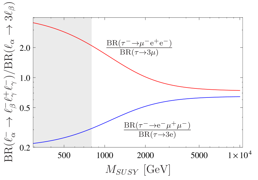
Figure 5: Ratios of 3-body $\tau$ decays as functions of $M_{SUSY}$ and $M_{R}$. The grey area is excluded by the ATLAS SUSY search [24].

Thus, these ratios can be used to pinpoint the dominant contribution and learn more about the mechanism at the origin of LFV. For completeness, we note that the branching ratios of $\tau^{-}\rightarrow\ell_{\gamma}^{-}\ell_{\beta}^{+}\ell_{\gamma}^{-}$ decays are strongly suppressed, at least by a factor of $10^{-6}$ with respect to the other 3-body decays, as they require an additional flavour violating vertex.

5 Conclusion

In this work, we provide for the first time a complete calculation of cLFV lepton decays and neutrinoless $\mu-e$ conversion in muonic atoms in the supersymmetric inverse seesaw, taking into account all SUSY and non-SUSY contributions. We have found that for small $M_{R}$ or large $M_{SUSY}$, the non-SUSY contributions dominate. In particular, for 3-body decays and $\mu-e$ conversion, the largest contributions come from boxes and Z-penguins which partially cancel each other, reducing the total branching ratio by up to one order of magnitude. In the large $M_{R}$ or small $M_{SUSY}$ regime, the SUSY contributions dominate, especially the $\gamma$-penguins. We expect these results to be quite generic and to hold for other low-scale seesaw models with right-handed neutrinos and nearly conserved lepton number. In fact, our findings agree with previous results in low-scale type I seesaw models [26, 27, 28, 29]. All types of observables can already be used to constrain the parameter space of the supersymmetric inverse seesaw. However, due to the huge improvements in experimental sensitivities expected in the upcoming years, the most promising observable depends on the time scale considered. In the short-term, it will be $\mu\rightarrow e\gamma$, while $\mu\rightarrow 3e$ should be the most constraining around 2016 and $\mu-e$ would give the most stringent limits around 2020. Finally, we have shown that ratios of 3-body $\tau$ decays will be extremely useful in finding the dominant contribution to cLFV processes.

References

- [1] D. Forero, M. Tortola, and J. Valle, (2014), arXiv:1405.7540.
- [2] R. Mohapatra, Phys.Rev.Lett. 56, 561 (1986).
- [3] R. Mohapatra and J. Valle, Phys.Rev. D34, 1642 (1986).
- [4] J. Bernabeu, A. Santamaria, J. Vidal, A. Mendez, and J. Valle, Phys.Lett. B187, 303 (1987).
- [5] Mu2e Collaboration, R. Abrams et al., Mu2e Conceptual Design Report, (2012), arXiv:1211.7019.
- [6] The PRISM/PRIME Group, An Experimental Search for A Conversion at Sensitivity of the Order of with a Highly Intense Muon Source: PRISM.
- [7] M. E. Krauss, W. Porod, F. Staub, A. Abada, A. Vicente and C. Weiland, Phys. Rev. D 90 (2014) 013008, arXiv:1312.5318.
- [8] A. Abada, M. E. Krauss, W. Porod, F. Staub, A. Vicente and C. Weiland, arXiv:1408.0138.
- [9] M. Gonzalez-Garcia and J. Valle, Phys.Lett. B216, 360 (1989).
- [10] MEG Collaboration, J. Adam et al., Phys.Rev.Lett. 110, 201801 (2013), arXiv:1303.0754.
- [11] A. Baldini et al., (2013), arXiv:1301.7225.
- [12] BaBar Collaboration, B. Aubert et al., Phys.Rev.Lett. 104, 021802 (2010), arXiv:0908.2381.
- [13] T. Aushev et al., (2010), arXiv:1002.5012.
- [14] SINDRUM Collaboration, U. Bellgardt et al., Nucl.Phys. B299, 1 (1988).
- [15] A. Blondel et al., (2013), arXiv:1301.6113.
- [16] K. Hayasaka et al., Phys.Lett. B687, 139 (2010), arXiv:1001.3221.
- [17] SINDRUM II Collaboration., C. Dohmen et al., Phys.Lett. B317, 631 (1993).
- [18] SINDRUM II Collaboration, W. H. Bertl et al., Eur.Phys.J. C47, 337 (2006).
- [19] DeeMe Collaboration, M. Aoki, AIP Conf.Proc. 1441, 599 (2012).
- [20] W. Porod, F. Staub and A. Vicente, Eur. Phys. J. C 74 (2014) 2992, arXiv:1405.1434.
- [21] J. Casas and A. Ibarra, Nucl.Phys. B618, 171 (2001), arXiv:hep-ph/0103065.
- [22] L. Basso et al., Comput.Phys.Commun. 184, 698 (2013), arXiv:1206.4563.
- [23] A. Abada, D. Das, A. Teixeira, A. Vicente, and C. Weiland, JHEP 1302, 048 (2013), arXiv:1211.3052.
- [24] ATLAS Collaboration, G. Aad et al., JHEP 1409 (2014) 176, arXiv:1405.7875.
- [25] A. Abada, D. Das and C. Weiland, JHEP 1203 (2012) 100, arXiv:1111.5836.
- [26] A. Ilakovac and A. Pilaftsis, Phys.Rev. D80, 091902 (2009), arXiv:0904.2381.
- [27] R. Alonso, M. Dhen, M. Gavela, and T. Hambye, JHEP 1301, 118 (2013), arXiv:1209.2679.
- [28] D. Dinh, A. Ibarra, E. Molinaro, and S. Petcov, JHEP 1208, 125 (2012), arXiv:1205.4671.
- [29] A. Ilakovac, A. Pilaftsis, and L. Popov, Phys.Rev. D87, 053014 (2013), arXiv:1212.5939.