Searching for A Generic Gravitational Wave Background via Bayesian Nonparametric Analysis with Pulsar Timing Arrays

Abstract

Gravitational wave background results from the superposition of gravitational waves generated from all sources across the Universe. Previous efforts on detecting such a background with pulsar timing arrays assume it is an isotropic Gaussian background with a power law spectrum. However, when the number of sources is limited, the background might be non-Gaussian or the spectrum might not be a power law. Correspondingly previous analysis may not work effectively. Here we use a method — Bayesian Nonparametric Analysis — to try to detect a generic gravitational wave background, which directly sets constraints on the feasible shapes of the pulsar timing signals induced by a gravitational wave background and allows more flexible forms of the background. Our Bayesian nonparametric analysis will infer if a gravitational wave background is present in the data, and also estimate the parameters that characterize the background. This method will be much more effective than the conventional one assuming the background spectrum follows a power law in general cases. While the context of our discussion focuses on pulsar timing arrays, the analysis itself is directly applicable to detect and characterize any signals that arise from the superposition of a large number of astrophysical events.

I Introduction

It has been 30 years since Sazhin Sazhin (1978) showed how gravitational waves could be directly detected by correlating the timing residuals of a collection of pulsars, i.e., a pulsar timing array Foster and Backer (1990). Such an “astronomical detector” is sensitive to gravitational waves of periods ranging from the interval between timing observations (weeks to months) to the duration of the observational data sets (years), and supermassive black hole binaries with masses of $\sim 10^{7}-10^{10}\mathrm{M_{\odot}}$ are the primary candidates of gravitational wave sources. Gravitational waves generated by a large number of such binaries would be superposed to form a background Sesana et al. (2008). The background has been traditionally assumed as a stochastic Gaussian process with a power law spectrum due to Central Limit Theorem (e.g. Hellings and Downs (1983); Jenet et al. (2005, 2006); van Haasteren et al. (2009, 2011)). This approximation might break down because the gravitational wave contribution to the pulsar timing signals may be dominated by the strongest sources, the number of which may not be sufficient enough to fulfill the requirement of Central Limit Theorem Ravi et al. (2012). Here we propose a methodology — Bayesian Nonparametric Analysis Ghosh and Ramamoorthi (2003); Hjort et al. (2010) — to analyze the pulsar timing array data set that potentially includes contribution from a generic gravitational wave background. This method will set strong constraints on the feasible patterns of the pulsar timing signals induced by the background we try to search from the data. It would investigate if the gravitational wave background is present and also estimate the parameters that characterize the background. We will see that when the non-Gaussianity of the background becomes non-negligible, our method is still efficacious while the conventional method assuming the background is Gaussian becomes much less effective.

In Section II, we discuss the characteristics of the gravitational wave background and its non-Gaussianity. In Section III, we describe a Bayesian nonparametric analysis of the pulsar timing array data. In Section IV, we illustrate the effectiveness of this analysis by applying it to several representative examples and compare the analysis with the conventional method assuming the background is Gaussian. Finally, we summarize our conclusion in Section V.

II Characteristics of Gravitational Wave Background

II.1 Pulsar Timing Residuals Induced by A Gravitational Wave Background

The evidence of gravitational waves is sought in pulsar timing residuals, which are the difference between a collection of pulse “time of arrival” (TOA) measurements of a pulsar timing array and the predicted pulse arrival times based on timing models Hobbs et al. (2010). A gravitational wave background results from the superposition of gravitational waves from a large number of sources; correspondingly, pulsar timing response to a gravitational wave background would be the sum of timing responses to gravitational waves from individual sources.

A plane gravitational wave propagating in direction $\hat{k}$ from a single source is represented by the transverse-traceless gauge metric perturbation Misner et al. (1973)

$$h_{lm}(t,\vec{x}) =h_{(+)}(t-\hat{k}\cdot\vec{x})e^{(+)}_{lm}+h_{(\times)}(t-\hat{k}\cdot\vec{x})e^{(\times)}_{lm}$$ (1)

where $e^{(A)}_{lm}$ is the polarization tensor. Following Finn and Lommen (2010), the $j$th pulsar timing response to such a plane gravitational wave can be written as

$$\tau_{j}(t)=\sum_{A=+,\times}\,F^{(A)}_{j}(\hat{k})\,\left[\tau_{(A)}(t)-\tau_{(A)}(t-L_{j}(1+\hat{k}\cdot\hat{n}_{j}))\right]$$ (2a)

where $$\tau_{(A)} h_{(A)}$$ is the integral of

$$\frac{\mathrm{d}\,\tau_{(A)}}{\mathrm{d}\,u}=h_{(A)}(u)$$ (2b)

and $$F^{(A)} j$$ is the pattern function of the th pulsar,

$$F^{(A)}_{j}(\hat{k})=-\frac{\hat{n}^{l}_{j}\hat{n}^{m}_{j}e^{(A)}_{lm}(\hat{k})}{2(1+\hat{k}\cdot\hat{n}_{j})}$$ (2c)

where $$\hat{n}^{l}_{j} j$$ is the direction from the Earth toward the th pulsar.

We can see that the gravitational wave contribution is the sum of two functionally identical terms, one time-shifted with respect to the other by an amount proportional to the Earth-pulsar distance along the wave propagation direction. The first term is referred to as the “Earth Term”, while the second is referred to as the “Pulsar Term.”

The $j$th Pulsar timing response to a gravitational wave background would be the sum of Eq. (2),

$$\tau_{j}(t)=\sum_{a}\sum_{A}\,F^{(A)}_{j}(\widehat{k_{a}})\,\left[\tau^{a}_{(A)}(t)-\tau^{a}_{(A)}(t-L_{j}(1+\widehat{k_{a}}\cdot\hat{n}_{j}))\right]$$ (3)

where $a$ labels the contribution from the $a$th source. We may express the right hand side of Eq. (3) in terms of its Fourier components:

$$\tau_{j}(t) =\sum_{a}\sum_{A}\,F^{(A)}_{j}(\widehat{k_{a}})\,\int\mathrm{d}f\,\left[\widetilde{\tau^{a}_{(A)}}(f)e^{i\,2\pi ft}-\widetilde{\tau^{a}_{(A)}}(f)e^{i\,2\pi f\left(t-L_{j}(1+\widehat{k_{a}}\cdot\hat{n}_{j})\right)}\right]$$

$$=\sum_{A}\int\mathrm{d}f\left[\sum_{a}F^{(A)}_{j}(\widehat{k_{a}})\widetilde{\tau^{a}_{(A)}}(f)e^{i\,2\pi ft}-\sum_{a}F^{(A)}_{j}(\widehat{k_{a}})\widetilde{\tau^{a}_{(A)}}(f)e^{-i\,2\pi fL_{j}(1+\widehat{k_{a}}\cdot\hat{n}_{j})}e^{i\,2\pi ft}\right]$$ (4)

We notice that compared with the Earth term, the Pulsar term has an extra phase $e^{-i\,2\pi fL_{j}(1+\widehat{k_{a}}\cdot\hat{n}_{j})}$. In pulsar timing array waveband, the pulsar distance is much longer than the gravitational wavelength, i.e., $fL_{j}\gg 1$. Correspondingly, when summing over the entire sky the Pulsar term vanishes and the pulsar timing response to a gravitational wave background, i.e., Eq. (3), can be simplified as

$$\tau_{j}(t)=\sum_{a}\sum_{A}\,F^{(A)}_{j}(\widehat{k_{a}})\,\tau^{a}_{(A)}(t)$$ (5)

II.2 Non-Gaussianity of the Gravitational Wave Background

The assumption of Gaussianity of the gravitational wave background results from Central Limit Theorem Feller (1945). However, the number of gravitational wave sources that can contribute to the pulsar timing array waveband is limited, which may not be sufficient to fulfill the requirement of the Central Limit Theorem Ravi et al. (2012). Here we use a toy model of gravitational wave source population to illustrate how the degree of non-Gaussianity increases as the number of gravitational wave sources decreases. We refer readers to Ravi et al. (2012) for details.

The degree of non-Gaussianity of a distribution is usually characterized by the skewness and kurtosis (e.g. Joanes and Gill (2002)). The skewness $\widehat{S}_{X}$ and the kurtosis $\widehat{K}_{X}$ of a random variable $X$ are respectively defined as Joanes and Gill (2002)

$$\widehat{S}_{X}=\frac{\langle\left(X-\langle X\rangle\right)^{3}\rangle}{\left(\langle\left(X-\langle X\rangle\right)^{2}\rangle\right)^{3/2}}$$ (6a)

$$\widehat{K}_{X}=\frac{\langle\left(X-\langle X\rangle\right)^{4}\rangle}{\left(\langle\left(X-\langle X\rangle\right)^{2}\rangle\right)^{2}}-3$$ (6b)

where $\langle\rangle$ denotes ensemble average. If $X$ is Gaussian distributed, the skewness $\widehat{S}_{X}$ and the kurtosis $\widehat{K}_{X}$ are both zero. Negative skewness indicates the left tail of the distribution is longer than the right one and positive skewness indicates the right tail is longer than the left one Joanes and Gill (2002); negative kurtosis indicates the distribution has shorter tails than Gaussian distribution and positive kurtosis indicates the distribution has longer tails than Gaussian distribution Joanes and Gill (2002). If $X$ is the sum of $n$ zero mean identically and independently distributed (i.i.d) random variables, i.e.,

$$X=\sum^{n}_{a}x_{a}$$ (7a)

with

$$\langle x\rangle=0$$ (7b)

then we can obtain

$$\langle X\rangle =0$$ (7c)

$$\langle(X-\langle X\rangle)^{2}\rangle =n\langle x^{2}_{a}\rangle$$ (7d)

$$\langle(X-\langle X\rangle)^{3}\rangle =n\langle x^{3}_{a}\rangle$$ (7e)

$$\langle(X-\langle X\rangle)^{4}\rangle =n\langle x^{4}_{a}\rangle+3n(n-1)(\langle x^{2}_{a}\rangle)^{2}$$ (7f)

where we have used the fact that the ensemble average of any quantity with a linear factor of $$x_{a} n$$ is zero. Correspondingly, when is large, we can express the skewness and kurtosis as

$$\widehat{S}_{X} =\frac{1}{\sqrt{n}}\frac{\langle x^{3}_{a}\rangle}{\left(\langle x^{2}_{a}\rangle\right)^{3/2}}$$ (7g)

$$\widehat{K}_{X} =\frac{1}{n}\frac{\langle x^{4}_{a}\rangle}{\left(\langle x^{2}_{a}\rangle\right)^{2}}$$ (7h)

We can see that as the number of the individual random variable $$x_{a}$$ goes to infinity, the skewness and kurtosis approach zero and the distribution becomes Gaussian. This is what Central Limit Theorem implies.

In the case of gravitational wave background, $X$ is the timing residual $\tau_{j}$ induced by the background in Eq. (5), and $x_{a}$ is the timing residuals induced by the $a$th single source. For simplicity, we assume that the supermassive black hole binaries are the primary sources of gravitational waves in pulsar timing array waveband. They are homogeneously and isotropically distributed in the sky, and their orbital evolution is driven by gravitational wave emission; correspondingly, the number of the binaries per frequency per comoving volume is Sesana et al. (2008)

$$\frac{\mathrm{d^{2}}N}{\mathrm{d}f\,\mathrm{d}V_{\mathrm{c}}}\propto f^{-11/3}$$ (8)

where $N$ denotes the number of the binaries; $f$ and $V_{\mathrm{c}}$ respectively denote gravitational wave frequency and comoving volume of the universe. We also assume that the gravitational waves generated by these sources are monochromatic waves Ellis et al. (2012a, b). We only consider gravitational waves with period $\lesssim 5\mathrm{yr}$, of which the induced peak pulsar timing residuals are above $0.01\,\mathrm{ns}$, since only these waves will significantly contribute to the pulsar timing residuals across $5$ year observation as the current International pulsar timing array (IPTA) Hobbs et al. (2010); Demorest et al. (2012); Manchester et al. . The gravitational waves with longer periods will be fitted out by the procedure in the standard pulsar timing analysis that removes the linear and quadratic trends induced by pulsar spin and spin down. In this range, the number of sources $N$ should be $\sim 10^{5}-10^{6}$ as expected from theoretical models Sesana et al. (2008, 2011).

To compute the skewness and kurtosis of timing residuals induced by a gravitational wave background, we can directly follow Eq. (7g) and Eq. (7h). The timing residual $\tau^{a}_{j}$ of the $j$th pulsar induced by the sinusoidal gravitational waves generated from the $a$th individual source would be

$$\tau^{a}_{j}(t) =F^{(+)}_{j}(\widehat{k_{a}})\,B^{a}_{(+)}\cos\left(2\pi f^{a}t+\phi^{a}\right)+F^{(\times)}_{j}(\widehat{k_{a}})\,B^{a}_{(\times)}\sin\left(2\pi f^{a}t+\phi^{a}\right)$$

$$=B^{a}_{j}\cos\left(2\pi f^{a}t+\phi^{a}+\psi^{a}_{j}\right)$$ (9a)

where $$B^{a}_{(A)} (A) f^{a} \phi^{a} B^{a}_{j} \psi^{a}_{j}$$ denotes the amplitudes of the timing residuals induced by polarization component; and are respectively the frequency and initial phase of the gravitational waves; and are respectively

$$B^{a}_{j} =\sqrt{[F^{(+)}_{j}\,B^{a}_{(+)}]^{2}+[F^{(\times)}_{j}\,B^{a}_{(\times)}]^{2}}$$ (9b)

$$\psi^{a}_{j} =\arctan\left[\frac{F^{(+)}_{j}\,B^{a}_{(+)}}{F^{(\times)}_{j}\,B^{a}_{(\times)}}\right]$$ (9c)

Assuming that the initial phase $\phi^{a}$ is uniformly distributed between $0$ and $2\pi$, we can obtain

$$\langle\tau^{a}_{j}\rangle =\langle B^{a}_{j}\rangle\,\langle\cos\left(2\pi f^{a}t+\phi^{a}+\psi^{a}_{j}\right)\rangle=0$$ (10a)

$$\langle\left(\tau^{a}_{j}\right)^{2}\rangle =\langle\left(B^{a}_{j}\right)^{2}\rangle\,\langle\cos^{2}\left(2\pi f^{a}t+\phi^{a}+\psi^{a}_{j}\right)\rangle=\pi\,\langle\left(B^{a}_{j}\right)^{2}\rangle$$ (10b)

$$\langle\left(\tau^{a}_{j}\right)^{3}\rangle =\langle\left(B^{a}_{j}\right)^{3}\rangle\,\langle\cos^{3}\left(2\pi f^{a}t+\phi^{a}+\psi^{a}_{j}\right)\rangle=0$$ (10c)

$$\langle\left(\tau^{a}_{j}\right)^{4}\rangle =\langle\left(B^{a}_{j}\right)^{4}\rangle\,\langle\cos^{4}\left(2\pi f^{a}t+\phi^{a}+\psi^{a}_{j}\right)\rangle=\frac{3\pi}{4}\,\langle\left(B^{a}_{j}\right)^{4}\rangle$$ (10d)

and following Eq. (7g) and Eq. (7h), the skewness and kurtosis of of timing residuals induced by a gravitational wave background would be

$$\widehat{S}_{\tau} =0$$ (10e)

$$\widehat{K}_{\tau} =\frac{1}{n}\frac{3}{4\pi}\frac{\langle\left(B^{a}_{j}\right)^{4}\rangle}{\left[\langle(B^{a}_{j})^{2}\rangle\right]^{2}}$$ (10f)

The amplitude $B^{a}_{j}$ depends on the pattern function, gravitational wave amplitudes and frequency. We can compute $\langle\left(B^{a}_{j}\right)^{2}\rangle$ and $\langle\left(B^{a}_{j}\right)^{4}\rangle$ by sampling an ensemble of the amplitude $B^{a}_{j}$ from the distribution Eq. (8) and numerically computing the ensemble average. Table 1 presents the skewness and kurtosis of timing residuals of PSR J1713+0747 induced by gravitational wave backgrounds respectively generated from $10^{6}$, $5\times 10^{5}$, $2\times 10^{5}$ and $10^{5}$ sources. As we stated above, all of these sources are generated in pulsar timing array waveband, i.e., their gravitational wave periods range from $3$ months to $5$ years. Their frequency distribution follows Eq. (8). For all these three gravitational wave backgrounds, about $0.1\%$ of the sources are responsible for $95\%$ of the residual power.

No. of Sources	skewness	kurtosis
$10^{6}$	0	0.01
$5\times 10^{5}$	0	0.02
$2\times 10^{5}$	0	0.05
$10^{5}$	0	0.1

Table 1: skewness and kurtosis of timing residuals induced by gravitational wave backgrounds respectively generated from $10^{6}$, $5\times 10^{5}$, $2\times 10^{5}$ and $10^{5}$ sources.

We can see that as the number of sources decreases, the degree of non-Gaussianity increases as implied by Central Limit Theorem. Correspondingly, the power law spectrum of the gravitational wave background as generally assumed would be effectively modified as it is derived based on the assumption that the number of sources are approximately infinite (e.g. Flanagan (1993); Jenet et al. (2005); van Haasteren et al. (2009)).

III Bayesian Nonparametric Analysis

To seek for the evidence of a gravitational wave background in the data set, we need to model its contribution to pulsar timing residuals. In principle, we can parameterize the pulsar timing response to a gravitational wave background by Eq. (5), i.e., superposition of gravitational waves from a large number of sources. In this way, the gravitational wave background is treated as a deterministic process rather than a stochastic one. However, such a parametric model will be computationally impossible due to the large number of parameters, because the gravitational wave signal induced by one single source requires about 10 to 20 parameters to characterize Ellis et al. (2012a, b), and correspondingly, to characterize a gravitational wave background generated by $\sim 10^{6}$ sources, the number of parameters will be $\sim 10^{7}$. To avoid both over-parameterization and strong assumption of Gaussianity, we introduce a different method — Bayesian nonparametric analysis Ghosh and Ramamoorthi (2003); Rasmussen and Christopher (2006); Hjort et al. (2010). This method also treats the gravitational wave background as a deterministic process since it originates from the superposition of gravitational waves from a finite number of sources, each of which is a deterministic process. However, we do not try to write down the exact deterministic function form. Instead, we assign a prior distribution on the function form of the signal, which will characterize the expected shape of the signal pattern, such as its smoothness, variation, trend, etc. These characteristics are used to represent the function form of the signal. Correspondingly, we are able to detect the signal whose deterministic function form has the same characteristics as what our prior distribution characterizes. For discussion of application of Bayesian nonparametrics in gravitational wave context, see Deng (2014); Lentati et al. (2014); Lee et al. (2014) for details.

III.1 Framework of Bayesian Nonparametric Analysis

To infer the pulsar timing residuals $\bm{\tau}$ induced by the gravitational wave background from a pulsar timing array data set $\bm{\mathrm{d}}$, we need to compute the posterior probability density $p(\bm{\tau}|\bm{\mathrm{d}})$, i.e., probability density of $\bm{\tau}$ given the data set $\bm{\mathrm{d}}$ Gelman et al. (2004). In this paper, we neglect other pulsar timing effects such as pulsar spin and spin down that would contribute to the data set $\bm{\mathrm{d}}$, and $\bm{\tau}$ only denotes the contribution from the gravitational wave background. It is straightforward to include other timing effects in our analysis by just adding a timing model to $\bm{\tau}$ like the way applied in van Haasteren et al. (2009).

Exploiting Bayes’ Theorem, the posterior probability density $p$ can be expressed in terms of the likelihood function $\Lambda$ , an a priori probability density $q$ that expresses the expectations of $\bm{\tau}$, and a normalization constant $Z$,

$$p(\bm{\tau}|\bm{\mathrm{d}})=\frac{\Lambda(\bm{\mathrm{d}}|\bm{\tau})\,q(\bm{\tau})}{Z(\bm{\mathrm{d}})}$$ (11)

where $\Lambda(\bm{\mathrm{d}}|\bm{\tau})$ is the likelihood function, which describes the probability of the data set $\bm{\mathrm{d}}$ given the signal characterized by $\bm{\tau}$; $q(\bm{\tau})$ is the a priori probability density of $\bm{\tau}$ that expresses our expectation before we obtain the data set; $Z(\bm{\mathrm{d}})$ is the normalization constant.

As shown in Finn and Lommen (2010); Deng (2014), the likelihood function is a multivariate Gaussian distribution of the data set $\bm{$},asthepulsartimingnoiseiswellmodelledaszeromeanGaussiandistributionsandtheyareuncorrelatedamongdifferentpulsars,i.e.,\begin{aligned} \Lambda(\bm{\mathrm{d}}|\bm{\tau})&=\prod^{N_{p}}_{j=1}\frac{\exp\left[-\frac{1}{2}(\mathrm{d}_{j}-\tau_{j})^{T}\mathrm{C}^{-1}_{j}(\mathrm{d}_{j}-\tau_{j})\right]}{\sqrt{(2\pi)^{\mathrm{dim}\,\mathrm{d}_{j}}\det||\mathrm{C}_{j}||}}\\ &=N(\bm{\mathrm{d}}-\bm{\tau}|\bm{\mathrm{C}})\end{aligned}where$N_p$isthenumberofpulsarsinthepulsartimingarray,and$C_j$isthenoisecovariancematrixofthe$j$thpulsar.\par Theaprioriprobabilitydensity$q(τ)$describesourexpectationsofthepulsartimingresidualsinducedbythegravitationalwavebackgroundbeforeanalyzingthedataset$d$,whichwillsetastrongconstraintonallpossibleformsof$q(τ)$wetrytoexplore\cite[cite]{\@@bibref{Authors Phrase1YearPhrase2}{Sudderth:2006:gmf}{\@@citephrase{(}}{\@@citephrase{)}}}.Undertheassumptionthatwedonothaveinformationonthevaluesof$τ$atinitialobservationtime,i.e.,thepriorof$τ$holdstimeinvariancesymmetry,itcanbeprovedthatthepriordistributionof$τ$isastationaryGaussianprocesswithzeromean\cite[cite]{\@@bibref{Authors Phrase1YearPhrase2}{summerscales:2008:mef, deng:2014:sfg, Bretthorst:1988:bsa}{\@@citephrase{(}}{\@@citephrase{)}}}\lx@equationgroup@subnumbering@begin\begin{aligned} q(\bm{\tau})&=\frac{\exp\left[-\frac{1}{2}\sum\limits_{j,k}\int\mathrm{d}t\,\mathrm{d}t^{\prime}\,\tau_{j}(t)\,\mathrm{K}^{-1}_{jk}(t,t^{\prime})\,\tau_{k}(t^{\prime})\right]}{\sqrt{(2\pi)^{\mathrm{dim}\mathrm{K}}\det||\mathrm{K}||}}\end{aligned}where$j,\,k$arepulsarindices;$\mathrm{K}$isacovariancefunctionorkernelofthestationaryGaussianprocessonlydependingonthetimedifference\cite[cite]{\@@bibref{Authors Phrase1YearPhrase2}{rasmussen:2006:gpf}{\@@citephrase{(}}{\@@citephrase{)}}},i.e.,\begin{aligned} &\mathrm{K}_{jk}(t,t^{\prime})=\mathrm{K}_{jk}(\Delta t)\end{aligned}where$\Delta t$denotes\begin{equation}\Delta t=|t-t^{\prime}|\end{equation}\par\lx@equationgroup@subnumbering@end Thekernelwillcharacterizethesmoothness,trendandvariationofthetimingresidualinducedbythegravitationalwavebackgroundandcorrespondinglysetstrongconstraintsonthepossibleshapesofit.Ingeneral,therewouldbesomenuisanceparametersinthekernel,whicharereferredtoas{\it hyperparameters}\cite[cite]{\@@bibref{Authors Phrase1YearPhrase2}{gelman:2004:bda}{\@@citephrase{(}}{\@@citephrase{)}}}.TodoafullBayesiananalysis,wealsoneedtoassignthepriorforthehyperparameters,i.e.,hyperpriors\cite[cite]{\@@bibref{Authors Phrase1YearPhrase2}{gelman:2004:bda}{\@@citephrase{(}}{\@@citephrase{)}}}.Thechoiceofkernelandhyperpriorwillbediscussedinthenextsubsection.\par$

III.2 The choice of Gaussian Process Prior

III.2.1 Prior of $\boldsymbol{\tau}$

As discussed above, the prior probability of the timing residuals induced by the gravitational wave background will constrain their feasible forms we try to explore, so the prior we choose should express the characteristics implied in Eq. (5).

Following Eq. (5), the timing residual induced by the superposition of gravitational waves from direction $\hat{k}$ can be written as

$$\tau_{\hat{k}}(t)=\sum_{A}\,F^{(A)}(\hat{k})\,\sum_{a\,(\hat{k})}\tau^{a}_{(A)}(t)$$ (13)

where $a\,(\hat{k})$ labels the sources located in $\hat{k}$ direction. To choose an appropriate Gaussian process prior of $\tau_{\hat{k}}$, we need to first find a Gaussian process prior of $\tau^{a}_{(A)}$ of a single source.

In pulsar timing array waveband, the single gravitational wave source could be a circular binary, an eccentric binary or a burst Hobbs et al. (2010). The dynamics of those gravitational wave sources are expected to be smooth Hobbs et al. (2010) and correspondingly, $\tau^{a}_{(A)}$ is expected to be a smooth function of time Deng (2014). As a consequence, the mean square of $\tau^{a}_{(A)}$ under its prior has to be infinitely differentiable, which requires the kernel of its stationary Gaussian process prior infinitely differentiable at $\Delta t=0$ Adler (1981). Only few kernels we know satisfy this requirement Stein (1999) and the one with the least number of hyperparameters is Rasmussen and Christopher (2006); Deng (2014)

$$\mathrm{K}_{a(A)}(\Delta t)=\sigma^{2}_{a(A)}\exp(-\frac{\Delta t^{2}}{2\,\lambda_{a}^{2}})$$ (14a)

and the corresponding Gaussian process prior of $$\tau^{a}_{(A)}$$ would be

$$q(\tau^{a}_{(A)})=\frac{\exp\left[-\frac{1}{2}\int\mathrm{d}t\,\mathrm{d}t^{\prime}\,\tau^{a}_{(A)}(t)\,\mathrm{K}^{-1}_{a(A)}(\Delta t)\,\tau^{a}_{(A)}(t^{\prime})\right]}{\sqrt{(2\pi)^{\mathrm{dim}\mathrm{K}}\det||\mathrm{K}||}}$$ (14b)

where $$\sigma_{a(A)} \tau^{a}_{(A)} a \lambda_{a} \lambda_{a} \tau^{a}_{(A)} \lambda_{a} \lambda_{a}$$ represents the rms amplitude from the th source and is the characteristic time-scale of the waveform. Within , is expected to cross the zero level only once Adler (1981). Therefore, for gravitational wave burst sources such as encounters of two supermassive black holes, characterizes the duration of the burst Deng (2014); and for gravitational waves from gravity-bound binaries, characterizes periods of the binaries.

Eq. (13) shows that $\tau_{\hat{k}}$ is the linear superposition of $\tau^{a}_{(A)}$ and we assume the two polarization components of the gravitational wave from a single source are independent; correspondingly, the kernel for the Gaussian process prior of $\tau_{\hat{k}}$ would be the linear superposition of Eq. (14a),

$$\mathrm{K}_{\hat{k}\,(jk)}(\Delta t) =\sum_{A}\,F_{j}^{(A)}(\hat{k})F_{k}^{(A)}(\hat{k})\,\sum_{a\,(\hat{k})}\sigma^{2}_{a(A)}\exp\left(-\frac{\Delta t^{2}}{2\,\lambda_{a}^{2}}\right)$$ (15a)

where $$j,\,k a\,(\hat{k}) \hat{k} \hat{k} \sigma_{a(A)} \sigma^{2}_{\hat{k}(A)} \lambda^{2}_{\hat{k}} \pi_{\hat{k}(A)}\left(\lambda^{2}_{k}\right) \lambda^{2}_{\hat{k}}$$ denote pulsar indices and denotes that the sum is over all sources in sky location . If we assume that at the sky location , total square sum of all source rms amplitude is and the density of the sources with square characteristic time-scale is , we can approximate the second sum in Eq. (15a) as an integral over all possible , i.e.,

$$\sum_{a\,(\hat{k})}\sigma^{2}_{a(A)}\exp\left(-\frac{\Delta t^{2}}{2\,\lambda_{a}^{2}}\right)=\sigma^{2}_{\hat{k}(A)}\,\int\mathrm{d}\lambda^{2}_{\hat{k}}\,\,\pi_{\hat{k}(A)}(\lambda^{2}_{\hat{k}})\,\exp\left(-\frac{\Delta t^{2}}{2\,\lambda^{2}_{\hat{k}}}\right)$$ (15b)

because the distribution of polarization angle is expected to be uniform Misner et al. (1973); Christensen (1992); Flanagan (1993), so $$\sigma^{2}_{\hat{k}(A)} \pi_{\hat{k}(A)}$$ and are the same for the two GW polarization components, i.e.,

$$\sigma^{2}_{\hat{k}(+)}=\sigma^{2}_{\hat{k}(\times)}=\sigma^{2}_{\hat{k}}$$ (15c)

$$\pi_{\hat{k}(+)}=\pi_{\hat{k}(\times)}=\pi_{\hat{k}}$$ (15d)

as a result, the kernel of the Gaussian process prior of $$\tau_{\hat{k}}$$ becomes

$$\mathrm{K}_{\hat{k}\,(jk)}(\Delta t)=\left(\sum_{A}\,F_{j}^{(A)}(\hat{k})F_{k}^{(A)}(\hat{k})\right)\,\sigma^{2}_{\hat{k}}\,\int\mathrm{d}\lambda^{2}_{\hat{k}}\,\,\pi_{\hat{k}}(\lambda^{2}_{\hat{k}})\,\exp\left(-\frac{\Delta t^{2}}{2\,\lambda^{2}_{\hat{k}}}\right)$$ (15e)

Because $\tau^{a}_{(A)}$ is expected to be a smooth function of time, and $\tau_{\hat{k}}$ is a linear superposition of a finite number of $\tau^{a}_{(A)}$, so $\tau_{\hat{k}}$ should also be a smooth function of time. Correspondingly, the kernel of its Gaussian process prior, i.e., Eq. (15e), should be infinitely differentiable at $\Delta t=0$ Adler (1981). This requirement sets a strong constraint on the choices of $\pi_{\hat{k}}$ and the one with the least number of parameters among the only few options is that $\pi_{\hat{k}}$ is an inverse gamma distribution of the square characteristic time-scale Stein (1999); Rasmussen and Christopher (2006),

$$\pi_{\hat{k}}(\lambda^{2}_{\hat{k}})=\frac{\beta_{\hat{k}}^{\alpha_{\hat{k}}}}{\Gamma(\alpha_{\hat{k}})}\lambda^{-2\alpha_{\hat{k}}-2}_{\hat{k}}\exp\left(-\frac{\beta_{\hat{k}}}{\lambda^{2}_{\hat{k}}}\right)$$ (16)

where $\alpha_{\hat{k}}$ and $\beta_{\hat{k}}$ are respectively referred to as shape parameter and the scale parameter, and they both have to be positive to guarantee $\pi_{\hat{k}}$ is normalizable Bernardo and Smith (2003); Gelman et al. (2004); $\Gamma(\alpha_{\hat{k}})$ is the gamma function of $\alpha_{\hat{k}}$ Abramowitz and Stegun (1964). Combining Eq. (15e) and Eq. (16), we can obtain the kernel of the Gaussian process prior of $\tau_{\hat{k}}$

$$\mathrm{K}_{\hat{k}\,(jk)}(\Delta t)=\sigma^{2}_{\hat{k}}\left(1+\frac{\Delta t^{2}}{2\alpha_{\hat{k}}\xi_{\hat{k}}^{2}}\right)^{-\alpha_{\hat{k}}}\,\sum_{A}\,F_{j}^{(A)}(\hat{k})F_{k}^{(A)}(\hat{k})$$ (17)

where $\xi_{\hat{k}}=\sqrt{\beta_{\hat{k}}}$, which is the characteristic time-scale of $\tau_{\hat{k}}$.

Because the gravitational wave background is the superposition of the gravitational waves from all directions in the sky, so kernel of the Gaussian process prior of the timing residuals induced by the background should be the sum of Eq. (17) across the whole sky. above, pulsar timing arrays can only localize the gravitational wave sources $\gtrsim 1000\,\mathrm{deg^{2}}$, which covers a few percent of the sky; correspondingly, we expect that the pulsar timing arrays should not be sensitive to the anisotropy of the gravitational wave background. We will demonstrate this point by representative examples in Sec. IV. In general, the gravitational wave sources may not be isotropically distributed and the anisotropy of the background can be characterized by decomposing the angular distribution of the gravitational wave energy density on the sky into multipole moments Mingarelli et al. (2013); Taylor and Gair (2013). However, for the purpose of demonstration, in this paper we only focus on the isotropic gravitational wave background and it is straightforward to generalize our method to anisotropic cases by combining the techniques presented in Mingarelli et al. (2013); Taylor and Gair (2013). By assuming isotropy, $\tau_{\hat{k}}$ in all directions will have the same $\sigma_{\hat{k}}$, $\alpha_{\hat{k}}$ and $\xi_{\hat{k}}$. Correspondingly, the kernel of the gravitational wave background induced timing residuals $\bm{\tau}$, i.e., Eq. (LABEL:eq:kernel0), is

$$\mathrm{K}_{jk}(\Delta t)=\sigma^{2}\left(1+\frac{\Delta t^{2}}{{2\alpha}\xi^{2}}\right)^{-\alpha}\,\gamma_{jk}$$ (18a)

where $$\gamma_{jk}$$ is

$$\gamma_{jk} =\int\mathrm{d^{2}}\Omega_{\hat{k}}\,\sum_{A}\,F_{j}^{(A)}(\hat{k})F_{k}^{(A)}(\hat{k})$$

$$=\frac{3}{2}\frac{1-\hat{n}_{j}\cdot\hat{n}_{k}}{2}\log\left(\frac{1-\hat{n}_{j}\cdot\hat{n}_{k}}{2}\right)-\frac{1}{4}\frac{1-\hat{n}_{j}\cdot\hat{n}_{k}}{2}+\frac{1}{2}+\frac{1}{2}\delta_{jk}$$ (18b)

We can see that $\gamma_{jk}$ is the Hellings-Downs Curve Hellings and Downs (1983).

Combining Eq. (III.1) and Eq. (18), we can obtain the Gaussian process prior of $\bm{\tau}$

$$q(\bm{\tau}|\sigma,\xi,\alpha)=\frac{\exp\left[-\frac{1}{2}\bm{\tau}^{T}\bm{\mathrm{K}}^{-1}\bm{\tau}\right]}{\sqrt{(2\pi)^{\mathrm{dim}\bm{\mathrm{K}}}\det||\bm{\mathrm{K}}||}}$$ (19)

where $\bm{\mathrm{K}}$ is expressed by Eq. (18)

III.2.2 Prior of Hyperparameters

The prior probability density of $\bm{\tau}$ Eq. (19) includes three undermined hyperparameters — $\sigma$, $\xi$ and $\alpha$, and we need to choose their prior probability density to make a full Bayesian inference.

For $\sigma$, it is a scale factor and we can choose Jeffreys prior Jeffreys (1946). However, Jeffreys prior will make the posterior probability density improper Deng (2014); Gelman (2006) and correspondingly such an uninformative prior is not an appropriate one. In this case, a uniform distribution from $0$ to $+\infty$, which will make the posterior distribution normalizable, is recommended Deng (2014); Gelman (2006), i.e.,

$$q_{\sigma}(\sigma)\propto 1$$ (20a)

For $\xi$, it is a time-scale factor and choose the Jeffreys prior

$$q_{\xi}(\xi)\propto 1/\xi$$ (20b)

The hyperparameter $\alpha$ is the shape parameter of the inverse gamma distribution Eq. (16), which represents the number density of the sources. We expect that the number of sources should monotonically increase with the increase of their periods or durations Sesana et al. (2008), correspondingly, $\pi_{\hat{k}}$ in Eq. (16) should be a monotonically increasing function of $\lambda_{\hat{k}}$. To satisfy this requirement, $\alpha$ should be between $0$ and $1$ Gelman et al. (2004); Bernardo and Smith (2003). Since $\alpha$ is a dimensionless hyperparameter, the corresponding uninformative prior should be a uniform distribution between $0$ and $1$ Bernardo and Smith (2003),

$$q_{\alpha}(\alpha)=1$$ (20c)

III.3 Bayesian Nonparametric Inferences

III.3.1 Inferring $\boldsymbol{\tau}$ and hyperparameters

Since we have obtained the likelihood function and chosen the appropriate priors for $\bm{\tau}$ and hyperparameters, we can follow the discussion in Sec. III.1 and make the inference of $\bm{\tau}$ and hyperparameters. Combining Eq. (11) with Eq. (III.1), Eq. (19) and Eq. (20), we can determine the joint posterior probability density of $\bm{\tau}$ and hyperparameters,

$$p(\bm{\tau},\sigma,\xi,\alpha|\bm{\mathrm{d}}) =\frac{1}{Z(\bm{\mathrm{d}})}\Lambda(\bm{\mathrm{d}}|\bm{\tau})q(\bm{\tau}|\sigma,\xi,\alpha)q_{\sigma}(\sigma)q_{\xi}(\xi)q_{\alpha}(\alpha)$$

$$=\sqrt{\frac{\det||\bm{\mathrm{A}}||}{(2\pi)^{\mathrm{dim}\bm{\mathrm{A}}}}}\exp\left[-\frac{1}{2}(\bm{\tau}-\bm{\tau}_{m})^{T}\bm{\mathrm{A}}(\bm{\tau}-\bm{\tau}_{m})\right]$$

$$\times\frac{1}{Z(\bm{\mathrm{d}})}\Lambda_{\theta}(\bm{\mathrm{d}}|\sigma,\xi,\alpha)q_{\sigma}(\sigma)q_{\xi}(\xi)q_{\alpha}(\alpha)$$ (21a)

where $$\bm{\mathrm{A}}$$ is

$$\bm{\mathrm{A}}=\bm{\mathrm{K}}^{-1}+\bm{\mathrm{C}}^{-1}$$ (21b)

and $$\bm{\tau}_{m}$$ satisfies

$$\bm{\mathrm{A}}\bm{\tau}_{m}=\bm{\mathrm{C}}^{-1}\bm{\mathrm{d}}$$ (21c)

$$\Lambda_{\theta}(\bm{\mathrm{d}}|\sigma,\xi,\alpha) \bm{\tau}$$ is the likelihood function of hyperparameters after marginalizing over :

$$\Lambda_{\theta}(\bm{\mathrm{d}}|\sigma,\xi,\alpha) =\int\Lambda(\bm{\mathrm{d}}|\bm{\tau})q(\bm{\tau}|\sigma,\xi,\alpha)\,\mathrm{d}\bm{\tau}$$

$$=\frac{\exp\left[-\frac{1}{2}\bm{\mathrm{d}}^{T}\bm{\mathrm{C}}^{-1}\bm{\mathrm{d}}\right]}{\sqrt{(2\pi)^{\mathrm{dim}\,\bm{\mathrm{d}}}\det||\bm{\mathrm{C}}||}}\times\frac{\exp\left[\frac{1}{2}(\bm{\mathrm{C}}^{-1}\bm{\mathrm{d}})^{T}\bm{\mathrm{A}}^{-1}(\bm{\mathrm{C}}^{-1}\bm{\mathrm{d}})\right]}{\sqrt{\det||\bm{\mathrm{A}}||\det||\bm{\mathrm{K}}||}}$$

$$=\frac{\exp\left[-\frac{1}{2}\bm{\mathrm{d}}^{T}(\bm{\mathrm{C}}+\bm{\mathrm{K}})^{-1}\bm{\mathrm{d}}\right]}{\sqrt{(2\pi)^{\mathrm{dim}\,\bm{\mathrm{d}}}\det||\bm{\mathrm{C}}+\bm{\mathrm{K}}||}}$$ (21d)

and the last row of Eq. (21) becomes the marginal posterior probability density of the hyperparameters:

$$p(\sigma,\xi,\alpha|\bm{\mathrm{d}})=\frac{1}{Z(\bm{\mathrm{d}})}\Lambda_{\theta}(\bm{\mathrm{d}}|\sigma,\xi,\alpha)q_{\sigma}(\sigma)q_{\xi}(\xi)q_{\alpha}(\alpha)$$ (21e)

Therefore, the Bayesian nonparametric analysis described above for detecting a gravitational wave background is identical to the Bayesian hierarchical modeling (e.g. Lentati et al. (2013)). We can see that the marginal likelihood function in Eq. (21) coincides the one used in previous methods that assume the gravitational wave background is generated from a Gaussian process with covariance matrix $\bm{\mathrm{K}}$. However, at the end of this section, we will discuss that different interpretations of the marginal likelihood in Eq. (21) will lead to different choices of $\bm{\mathrm{K}}$.

Eq. (21) summarizes Bayesian nonparametric inference, which gives estimation on $\bm{\tau}$ and hyperparameters.

III.3.2 Inferring the Presence of A Gravitational Wave Background

Given timing residual observations $\bm{\mathrm{d}}$ from an array of pulsars, we would like to infer if a gravitational wave background is present. We treat this question as a problem in Bayesian model comparison Gelman et al. (2004). Consider the two models

$$M_{1}=\left(\text{a gravitational wave background is present in the data set}\right)$$ (22a)

$$M_{0}=\left(\text{no gravitational waves backgrounds are present in the data set}\right)$$ (22b)

The purpose of model comparison is to check which model data favors. If data favors $M_{1}$, then it indicates that a gravitational wave is likely to be present in the data set. Bayes factor is often used for the criterion of this model comparison problem. However, if the prior distribution of the parameters is improper, there would be an arbitrary multiplicative factor in Bayes factor, which makes it ill-defined Kass and Raftery (1995); Gelman et al. (2004); Deng (2014). Correspondingly, Bayes factor may not be a suitable criterion for our case, because the prior distributions of RMS amplitude $\sigma$ and the characteristic time-scale $\xi$ are improper. Therefore, we use an alternative criterion Deviance Information Criterion (DIC) Spiegelhalter et al. (2002), which is the sum of two terms — one term represents “goodness of fitting”, which measures how well the model fits the data; the other term represents “the penalty of complexity”, which measures how complex the model is Claeskens and Hjort (2008). Here we briefly summarize the principle of DIC. We refer readers to Spiegelhalter et al. (2002) for detail discussion in general and Deng (2014) for application in gravitational wave context. Deng (2014) also discussed why DIC is more applicable than the commonly used Bayes factor in gravitational wave context.

In DIC, the “goodness of fitting” is summarized in “deviance”, defined as $-2$ times the log-likelihood Gelman et al. (2004):

$$D(\bm{\mathrm{d}},\bm{\tau})=-2\log\Lambda(\bm{\mathrm{d}}|\bm{\tau})$$ (23)

which measures the model discrepancy and resembles the classical $\chi^{2}$ goodness-of-fit measure. The average of the deviance on posterior probability distribution provides a summary of the error of model $M_{1}$ and represents “goodness of fitting” Spiegelhalter et al. (2002):

$$D_{\mathrm{avg}}(\bm{\mathrm{d}},M_{1})=\int D(\bm{\mathrm{d}},\bm{\tau})p_{\tau}(\bm{\tau}|\bm{\mathrm{d}})\mathrm{d}\bm{\tau}$$ (24a)

where $$p_{\tau}(\bm{\tau}|\bm{\mathrm{d}})$$ is the posterior probability density in Eq. (21) marginalizing over all hyperparameters:

$$p_{\tau}(\bm{\tau}|\bm{\mathrm{d}})=\int\,p(\bm{\tau},\sigma,\xi,\alpha|\bm{\mathrm{d}})\,\mathrm{d}\sigma\mathrm{d}\xi\mathrm{d}\alpha$$ (24b)

For model $M_{0}$, since there are no parameters representing the model, the average of the deviance is

$$D_{\mathrm{avg}}(\bm{\mathrm{d}},M_{0})=-2\log\Lambda(\bm{\mathrm{d}}|M_{0})$$ (25a)

where $$\Lambda(\bm{\mathrm{d}}|M_{0})$$ is the null model likelihood function

$$\Lambda(\bm{\mathrm{d}}|M_{0})=N(\bm{\mathrm{d}}|\bm{\mathrm{C}})=\frac{\exp\big{(}-\frac{1}{2}\bm{\mathrm{d}}^{T}\bm{\mathrm{C}}^{-1}\bm{\mathrm{d}}\big{)}}{\sqrt{(2\pi)^{\mathrm{dim}\,\bm{\mathrm{d}}}\det||\bm{\mathrm{C}}||}}$$ (25b)

Now we need to consider the complexity of a model and the more complex model with more adjustable parameters should have larger penalty Gelman et al. (2004); Claeskens and Hjort (2008); Jefferys and Berger (1991). The complexity of a model is represented by the measure of the degree of overfitting. In DIC, it is defined as the difference between the posterior mean deviance Eq. (24a) and the deviance at the mean value of $\bm{\tau}$ under its posterior probability distribution Eq. (24b) for model $M_{1}$ Spiegelhalter et al. (2002)

$$p_{D}(\bm{\mathrm{d}},M_{1})=D_{\mathrm{avg}}(\bm{\mathrm{d}},M_{1})-D(\bm{\mathrm{d}},\bar{\bm{\tau}})$$ (26a)

where $$\bar{\bm{\tau}} \bm{\tau}$$ is the mean value of under its posterior probability distribution Eq. (24b),

$$\bar{\bm{\tau}}=\int\,\bm{\tau}\,p_{\tau}(\bm{\tau}|\bm{\mathrm{d}})\,\mathrm{d}\bm{\tau}$$ (26b)

$p_{D}$ can be thought as the reduction in the lack of fit due to Bayesian estimation, or alternatively the degree of overfitting due to $\bar{\bm{\tau}}$ adapting to the data set $\bm{\mathrm{d}}$ Spiegelhalter et al. (2002), since $\bar{\bm{\tau}}$ serves as a Bayesian estimator of the model, and correspondingly $D(\bm{\mathrm{d}},\bar{\bm{\tau}})$ represents the lack of fit to the data due to the Bayesian estimation of the model.

For model $M_{0}$, since no parameters or functions are needed, so the effective number of parameters for this model, $p_{D}(\bm{\mathrm{d}},M_{0})$, is zero.

The sum of the average of the deviance and the effective number of parameters $p_{D}$ is referred to as Deviance Information Criterion Spiegelhalter et al. (2002),

$$\mathrm{DIC}(\bm{\mathrm{d}},M)=D_{\mathrm{avg}}(\bm{\mathrm{d}},M)+p_{D}(\bm{\mathrm{d}},M)$$ (27)

The data favors the model with smaller DIC, since such a model has smaller discrepancy of the data and is less complex.

The difference between the DICs of two models in Eq. (22) ,

$$\Delta\mathrm{DIC}=\mathrm{DIC}(\bm{\mathrm{d}},M_{1})-\mathrm{DIC}(\bm{\mathrm{d}},M_{0})$$ (28)

characterizes the relative odds between the two models. Therefore, the difference of DICs between two models is similar to likelihood ratio test statistic Neyman and Pearson (1933) and twice the natural logarithm of Bayes factor Kass and Raftery (1995). Correspondingly, it has the same scale as those statistics Spiegelhalter et al. (2002). If $\Delta\mathrm{DIC}\lesssim-10$, it is safe to conclude that the data strongly favors $M_{1}$ and there is strong evidence that a gravitational wave background is present in the data set Spiegelhalter et al. (2002).

III.4 Discussion of Deterministic and Stochastic Modeling

At this point, it is worth comparing the deterministic modeling by Bayesian nonparametrics discussed above and the stochastic modeling used by previous methods.

In general, when we detect a signal across a finite time duration, we have two ways to model the signal:

• assume the signal is generated by a deterministic process. However, we do not know the function form of the signal, on which we need to assign a prior distribution. This is what we did in this paper.

• assume the signal is a random sample (one single realization) generated from a stochastic process, and what we need to do is to model the distribution function of the stochastic process. This is what previous methods did.

Because we do not have an ensemble of the signals and we cannot reverse time to repeat the detection, so both of these modeling methods may lead to reasonable characterizations of the signal. Which is more effective depends on which model fits the data better, i.e., which method leads to a larger likelihood or a smaller DIC.

In the case of detecting a gravitational wave background, both of these two methods would result in the same marginal likelihood function Eq. (21), because in the first method, we assume the prior distribution of the signal form is a Gaussian distribution, and in the second method, we assume that the distribution function of the gravitational wave background is also a Gaussian distribution. This means that both of these two methods may lead to the same inference of the signal. So in practice, the method we present above may be considered as the same method as previous ones in van Haasteren et al. (2009); Lentati et al. (2013) except the difference choices of the kernel $\bm{\mathrm{K}}$. However, the choices of the kernels strongly depend on what logic we follow, which will lead to different values of likelihood functions. This is the key difference between the method presented here and the previous methods.

When we follow the first approach, as described in Section III.2.1, the kernel $\bm{\mathrm{K}}$, which originally appears in the prior distribution, is chosen to characterize the expected shape of the signal, such as its smoothness, its variation, its trend, etc. We use these characteristics to represent the underlying unknown deterministic function form of the signal. Following this logic, we finally obtain the appropriate kernel Eq. (18). While if we follow the second approach, $\bm{\mathrm{K}}$ characterizes the covariance of the Gaussian distribution, which is assumed to be the underlying distribution function of the gravitational wave background. Following this logic, $\bm{\mathrm{K}}$ would have to be the Fourier transform of a frequency power law, because it can be derived from physics that the frequency distribution of the gravitational wave sources follows a power law van Haasteren et al. (2009); Lentati et al. (2013). Using the first method cannot lead to the choice of a power law spectrum while using the second method cannot lead to the choice of Eq. (18). The two different choices of $\bm{\mathrm{K}}$ would lead to different values of the likelihood functions.

If the non-Gaussian part of the distribution of the gravitational wave background is significant, the second method will be ineffective because it only characterizes the covariance of the distribution but ignores the skewness, kurtosis and other parts of the distribution. We may wonder how the first method can be applied here. The first method does not try to characterize the underlying distribution of the gravitational wave background. The signal we detect is only one single sample (one single realization) generated from the underlying distribution, and without an ensemble of the signals, we may be hardly able to characterize the underlying distribution. Instead, the first method assumes the signal is just a representation of some deterministic function but does not worry if there is some underlying distribution. However, since we do not know the exact function form of the signal, we assign a prior distribution with a specific kernel to characterize the expected shape of the signal. Correspondingly, no matter if the signal is sampled from some distribution or what the distribution is, as long as our Gaussian prior with a kernel correctly characterizes the shape of the signal pattern, such as its smoothness, variation, trend, etc., our method would lead to a good inference of the signal.

To recap, even though for detecting a gravitational wave background, the deterministic modeling by our Bayesian nonparametrics and the previous stochastic modeling will lead to likelihood functions with the same form, our method only tries to characterize the signal itself and the kernel in the Gaussian prior distribution represents our expectation of the shape of the signal pattern; while previous methods assume the signal is sampled from some underlying distribution and try to use a Gaussian model with a power-law spectrum to characterize the distribution. These two approaches will lead to different choices of the kernels, which correspondingly would result in different values of likelihood functions.

IV Examples

IV.1 Overview

To illustrate the effectiveness of the analysis techniques described above, we apply them to simulated data sets of 4 millisecond pulsars in the current International Pulsar Timing Array (IPTA) Hobbs et al. (2010); Demorest et al. (2012); Manchester et al. which are most accurately timed as described in Table 2. The capability of detecting and characterizing gravitational waves is dominated by these best pulsars, although they are the minority of the full IPTA Burt et al. (2011). We will also compare our method to the conventional one proposed by van Haasteren et al van Haasteren et al. (2009), which assumes the background is exactly Gaussian .

Table 2:     4 IPTA pulsars we use, Their white timing noise rms and the Telescopes from which the timing residuals are measured Hobbs et al. (2010); Demorest et al. (2012); Manchester et al.

Pulsar	rms (ns)	Telescope
J1713$+$0747	30	AO
J1909$-$3744	38	GBT
J0437$-$4715	75	Parkes
J1857$+$0943	111	AO

We uniformly sample $50$ observation times across $5$ year observation, and the corresponding pulsar timing data sets are constructed by

• evaluating the pulsar timing residuals induced by a simulated gravitational wave background that will be described in Sec. IV.2.1.

• adding pulsar timing noise that will be described in Sec. IV.2.2 to the timing residuals obtained by the first step.

• removing the linear trend of the timing residuals obtained above to simulate the procedure in the standard pulsar timing analysis that removes the effects of pulsar spin and spin down.

When we analyze the data, we add a linear model in the pulsar timing response function to account for the linear trend, the same as the analysis in van Haasteren et al. (2009). We will also apply our analysis methods to a data set composed of timing noise alone for comparative study.

IV.2 Construction of Simulated data Sets

IV.2.1 Simulated Gravitational Wave Background

We construct the simulated observations of two isotropic gravitational wave backgrounds respectively generated from $10^{6}$ and $10^{5}$ supermassive black hole binaries. Both of these sources are generated in the same way as we did in Section II.2:

• the frequency distribution of these sources follows Eq. (8) with lower bound of $0.2\,\mathrm{yr}^{-1}$ and upper bound of $4\,\mathrm{yr}^{-1}$.

• all of these sources are uniformly distributed across the sky with their gravitational wave peak timing residuals ranging from $0.01\mathrm{ns}$ to $100\mathrm{ns}$.

• the orbital orientations and initial phases of all these sources are uniformly distributed.

• the timing residuals induced by the gravitational wave background are the sum of all the gravitational wave signals generated from the sources sampled from the distribution described in the above three steps. The RMS values of the gravitational wave amplitudes of the two gravitational wave backgrounds are both about $22\mathrm{ns}$.

The degrees of non-Gaussianity of these two backgrounds are presented in Table 1, and we can see the background with $10^{5}$ sources is more non-Gaussian than that with $10^{6}$ sources. For these two cases of simulated backgrounds, we will compare the results of our method and the conventional one proposed by van Haasteren et al van Haasteren et al. (2009) and we will see that our method is much more effective on the case of the background with $10^{5}$ sources.

IV.2.2 Pulsar Timing Noise

The millisecond pulsars used in current International pulsar timing array typically show white noise on short timescales, and few of them turn to red noise on timescales $\gtrsim 5$ years Demorest et al. (2012); Manchester et al. . For demonstrations, we use the noise model described in Deng (2014) and we briefly summarize it here. The power spectral density is taken to be Coles et al. (2011)

$$S_{n}(f)=\sigma^{2}_{n}+\sigma^{2}_{n}\left[\frac{1+\left(\frac{f}{f_{0}}\right)^{2}}{1+\left(\frac{f_{r}}{f_{0}}\right)^{2}}\right]^{-5/2}$$ (29a)

where

$$\sigma_{n} =\left(\text{white noise rms}\right)$$ (29b)

$$f_{r} =\left(\text{red-white noise cross-over frequency, $0.2\,\mathrm{yr^{-1}}$}\right)$$ (29c)

and $f_{0}$ softens the noise spectrum at ultra-low frequency. As long as $f_{0}$ is much less than the pulsar timing array frequency band, its value does not matter. In the simulation we set $f_{0}$ equal to $0.01\mathrm{nHz}$. We choose the power index of the red noise spectrum as $-5$ because the few millisecond pulsars showing red noise have noise spectrum with power index $-5$ Shannon and Cordes (2010).

The covariance matrix of the noise will be the fourier transform of the noise specturm density Eq. (29a) to time domain, i.e.,

$$\mathrm{C}(t_{i},\,t_{j})=\sigma^{2}_{n}\left(\delta_{ij}+\sqrt{\frac{2}{9\pi}}\left[1+\left(\frac{f_{r}}{f_{0}}\right)^{2}\right]^{5/2}f^{3}_{0}|t_{i}-t_{j}|^{2}K_{2}(f_{0}|t_{i}-t_{j}|)\right)$$ (30)

where $t_{i,j}$ are the “observation times” and $K_{2}$ is the modified Bessel function of the second kind with index $2$. The pulsar timing noise for each pulsar are sampled from multivariate normal distribution with zero mean and covariance matrix Eq. (30).

IV.3 Analysis of Simulated Data Sets

Our Bayesian nonparametric analysis is designed to investigate if a gravitational wave background is present in the dataset, and also infer the hyperparameters. We use Metropolis-Hasting method of Markov Chain Monte Carlo Robert and Casella to compute the posterior probability densities and Deviance Information Criterion described in Sec. III.3. We follow the same computing procedure as in van Haasteren et al. (2009) to sample the posterior probability distribution Eq. (21e) of the three hyperparameters, except we use the Cauchy distribution as the proposal distribution. We sample $10^{6}$ step random walks by Metropolis algorithm and it takes about three hours for analysis of each data set described above.

We apply both our method and the conventional Gaussian method on the two data sets — one contains the contribution of the gravitational wave background with $10^{6}$ sources and the other contains the contribution of the background with $10^{5}$ sources. We also analyze the data set consisting of timing noise alone only by our method for comparative study. Table 3 lists the results of the analysis. The parentheses in the second column contain the DIC differences obtained by applying conventional Gaussian method in van Haasteren et al. (2009).

Table 3:   Results for Bayesian Nonparametric Analysis on 3 Simulated Data Sets

No. of Sources	$\Delta\mathrm{DIC}$ (Gaussian)	$\epsilon_{\sigma}$	$\epsilon_{\xi}$	$\epsilon_{\alpha}$
$10^{6}$	-15 (-12)	$27.4\%$	$96.8\%$	$32.0\%$
$10^{5}$	-14 (-3)	$29.2\%$	$71.9\%$	$34.2\%$
Absent	5 (5)	$92.5\%$	$63.5\%$	$54.6\%$

Notes. The signals correspond to an isotropic gravitational wave background and an anisotropic one described in Sec. IV.2.1. $\epsilon_{\sigma}$, $\epsilon_{\xi}$ and $\epsilon_{\alpha}$ respectively denote the fractional uncertainty of $\sigma$, $\xi$ and $\alpha$. The parentheses contain the DIC differences by applying the conventional Gaussian method on the same data sets.

IV.3.1 Signal of an Isotropic Gravitational Wave Background with $10^{6}$ Sources

We simulate an isotropic gravitational wave background by sampling $10^{6}$ sources from a homogeneous and isotropic distribution Eq. (8) and computing the superposition of the timing residuals induced by the gravitational waves from them, as described in Sec. IV.2.1. The first row of Table. 3 and Fig. 1 summarize the results of our Bayesian nonparametric analysis:

• From the first row of Table. 3, we see that the difference between the DICs of the positive hypothesis and null hypothesis, described in Sec. III.3.2, is $-15$, corresponding to a strong evidence for the presence of a gravitational wave background in the data set. We apply the conventional Gaussian method in van Haasteren et al van Haasteren et al. (2009)on the same data set and the DIC difference is $-12$, which also indicates a strong evidence of the presence of a gravitational wave background. Therefore, the number of sources in this cases is not small enough to distinguish the effectiveness of the two analysis methods.

• We also infer the hyperparameters and Fig. 1 shows the posterior probability density of them. The mean value of $\sigma$ is $22.5\,\mathrm{ns}$ (consistent with the simulated signal of RMS amplitude 22ns) and its rms errors are respectively $6.2\,\mathrm{ns}$. Correspondingly, its fractional uncertainty is $27.4\%$. For $\xi$, the mean value is $0.25\,\mathrm{yr}$ and the rms error is $0.24\,\mathrm{yr}$, and the corresponding fractional uncertainty is $96.8\%$. We cannot measure the shape parameter $\alpha$ very well and it tends to be $1$. The mean and rms error are respectively $0.69$ and $0.22$, and the fractional error is $32.0\%$. Fig. 2 shows the posterior probability density of the strain amplitude $\sigma_{\mathrm{GW}}$ and the spectrum power index $\alpha_{\mathrm{GW}}$ the gravitational wave background obtained by applying the conventional method in van Haasteren et al. (2009).

  

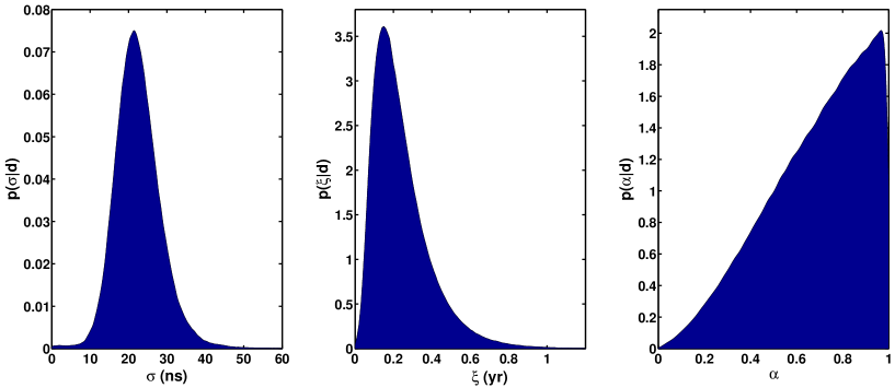
  Figure 1: Posterior probability densities of 3 hyperparameters — $\sigma$, $\xi$ and $\alpha$, for analysis on the data described in Sec. IV.3.1. The fractional errors of them are respectively $27.4\%$, $96.8\%$, $32.0\%$

  

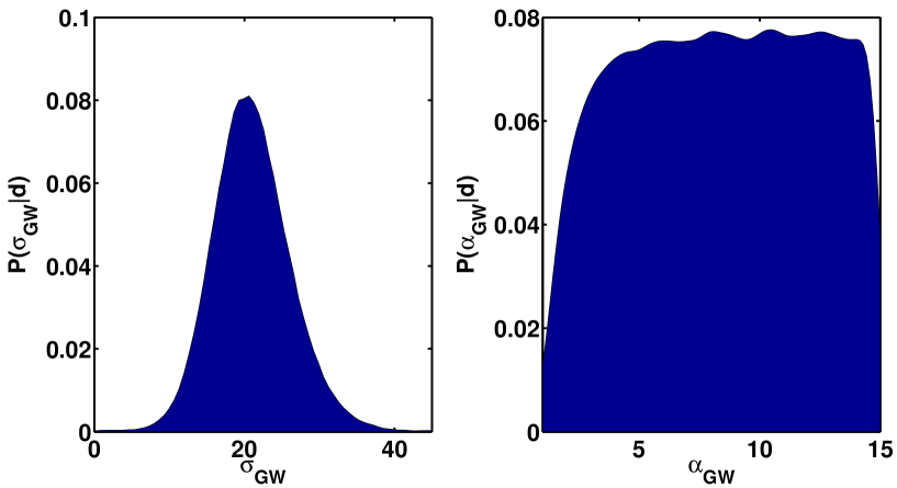
  Figure 2: Posterior probability densities the strain amplitude $\sigma_{\mathrm{GW}}$ and the spectrum power index $\alpha_{\mathrm{GW}}$ the gravitational wave background with $10^{6}$ sources obtained by applying the conventional method in van Haasteren et al. (2009).

IV.3.2 Signal of an Isotropic Gravitational Wave Background with $10^{5}$ Sources

We simulate an isotropic gravitational wave background by sampling $10^{5}$ sources from a homogeneous and isotropic distribution Eq. (8) and computing the superposition of the timing residuals induced by the gravitational waves from them, as described in Sec. IV.2.1. The degree of non-Gaussianity of this background is greater than the one with $10^{6}$ sources as illustrated in Table 1. The second row of Table. 3 and Fig. 3 summarize the results of our Bayesian nonparametric analysis on such “anisotropic signal” data:

• From the second row of Table. 3, we see that the difference between the DICs of the positive hypothesis and null hypothesis, described in Sec. III.3.2, is $-14$, corresponding to a strong evidence for the presence of a gravitational wave background in the data set. When we apply the conventional Gaussian method in van Haasteren et al. (2009) on the data set, we obtain a DIC difference of only $-3$, which indicates no strong evidence of a gravitational wave background. Therefore, the non-Gaussianity of this background is non-negligible, and our method shows the strong advantage over the conventional one in this case.

• We also infer the hyperparameters and Fig. 3 shows the posterior probability density of them. The mean value of $\sigma$ is $22.4\,\mathrm{ns}$ (consistent with the simulated signal of RMS amplitude 22ns) and its rms errors are respectively $6.5\,\mathrm{ns}$. Correspondingly, its fractional uncertainty is $30.0\%$. For $\xi$, the mean value is $0.36\,\mathrm{yr}$ and the rms error is $0.26\,\mathrm{yr}$, and the corresponding fractional uncertainty is $71.9\%$. We cannot measure the shape parameter $\alpha$ very well either and it also tends to be $1$. The mean and rms error are respectively $0.67$ and $0.23$, and the fractional error is $34.2\%$. Fig. 4 shows the posterior probability density of the strain amplitude $\sigma_{\mathrm{GW}}$ and the spectrum power index $\alpha_{\mathrm{GW}}$ the gravitational wave background obtained by assuming the background is Gaussian and applying the conventional method in van Haasteren et al. (2009).

  

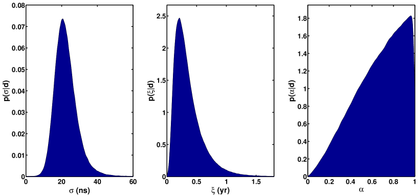
  Figure 3: Posterior probability densities of 3 hyperparameters — $\sigma$, $\xi$ and $\alpha$, for analysis on the data described in Sec. IV.3.2. The fractional errors of them are respectively $30.0\%$, $71.9\%$, $34.2\%$

  

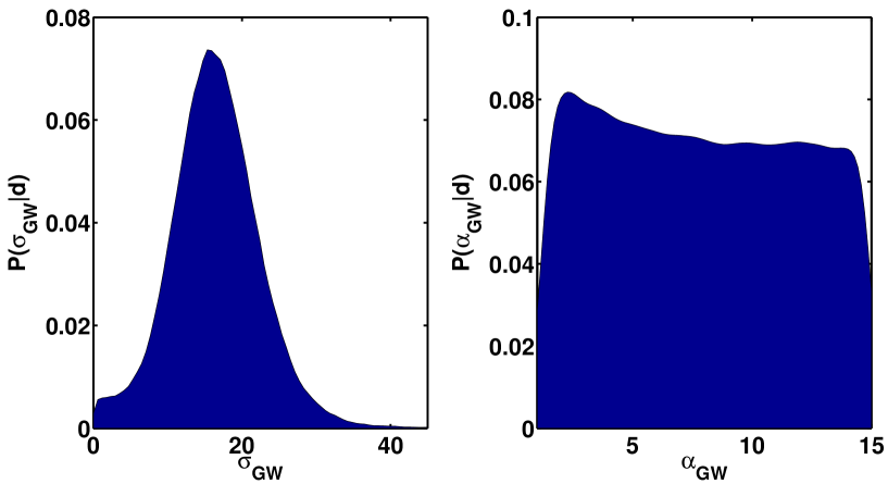
  Figure 4: Posterior probability densities the strain amplitude $\sigma_{\mathrm{GW}}$ and the spectrum power index $\alpha_{\mathrm{GW}}$ the gravitational wave background with $10^{5}$ sources obtained by assuming the background is Gaussian and applying the conventional method in van Haasteren et al. (2009).

IV.3.3 No Signal

For comparative study, we also apply our Bayesian nonparametric analysis to a data set with timing noise alone. The third row of Table. 3 and Fig. 5 summarize the results. The difference between the DICs of the two repulsive hypothesis is $5$, which shows that data favors the null hypothesis. All the hyperparameters are imprecisely determined. The method in van Haasteren et al. (2009) also offers a DIC difference of $5$.

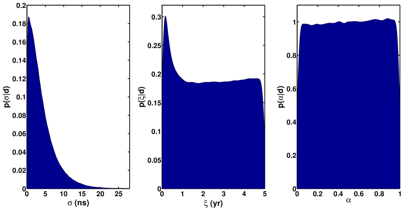
Figure 5: Posterior probability densities of 3 hyperparameters — $\sigma$, $\xi$ and $\alpha$, for analysis on the noise alone data described in Sec. IV.3.3. The fractional errors of them are respectively $92.5\%$, $63.5\%$, $54.6\%$

V Conclusion

First detection of gravitational waves will open a new window of our universe complementary with the conventional electromagnetic astronomy. Due to their unique nature, to detect gravitational waves do not only requires more sensitive and innovative instruments, but it also demands more advanced analysis methodology and techniques. In this paper, we use a Bayesian nonparametric method to analyze the pulsar timing array data set which may contain contribution from a gravitational wave background originated from the superposition of gravitational waves generated by supermassive black hole binaries in the universe. .

When the number of the gravitational wave sources that significantly contribute to pulsar timing signals is small, the previous methods based on the assumption that the background spectrum is a power law may be restrictive. In order to detect a generic gravitational wave background, we treat it as a deterministic process rather than a stochastic one as before, since each gravitational wave from a single source is a deterministic process. Instead of parameterizing gravitational wave from each single source, we use a different method — Bayesian nonparametrics — to avoid the over-parameterization. In this way, we set strong constraints on the feasible shapes of the pulsar timing residuals induced by the background. We have found that our method works efficiently for theoretically expected signals. When the number of gravitational wave sources becomes small and the assumption of power law spectrum becomes ineffective, our method is still able to detect and characterize the signal while the conventional method becomes less effective.

For the purpose of demonstration, we apply our Bayesian nonparametric analysis to the pulsar timing data of the 4 best millisecond pulsars in current International pulsar timing array (IPTA), as the capability of detection and characterization of gravitational waves will be dominated by these pulsars Burt et al. (2011). However, our analysis can be straightforwardly applied to analyze the data of all the pulsars in IPTA. In the future, the effective number of pulsars whose timing noises are low enough to detect gravitational waves is expected to significantly increase with the birth of more sensitive radio telescopes such as Five-hundred-meter Aperture Spherical Telescope Nan et al. (2011) and Square Kilometer Array (SKA) Dewdney et al. (2009). Applying our analysis method to the pulsar timing data collected by these future telescopes will significantly improve the detection sensitivity and inference of the signals. While the context of our discussion focuses on pulsar timing arrays, the analysis itself is directly applicable to detect and characterize any signals that arise from the superposition of a large number of astrophysical events, such as detecting high frequency gravitational wave background by LIGO Abadie et al. (2012).