Membranes with a symmetry of cohomogeneity one

Abstract

We study the dynamics of the Nambu-Goto membranes with cohomogeneity one symmetry, i.e., the membranes whose trajectories are foliated by homogeneous surfaces. It is shown that the equation of motion reduces to a geodesic equation on a certain manifold, which is constructed from the original spacetime and Killing vector fields thereon. A general method is presented for classifying the symmetry of cohomogeneity one membranes in a given spacetime. The classification is completely carried out in Minkowski spacetime. We analyze one of the obtained classes in depth and derive an exact solution.

I Introduction

Extended objects come out in various areas of physics: topological defects in field theories and in condensed matter physics, and branes in string theories, recently. In cosmology, topological defects such as cosmic strings and domain walls are supposed to have formed in the early universe. In the brane-world universe models, the universe itself is an extended object embedded in a bulk space Randall:1999ee . Recently, configuration of extended objects in black hole spacetimes are also of growing importance in discussions of strong coupling regime of gauge theories through gauge/gravity duality Maldacena:1997re .

Extended objects, compared with particles, have a wide variety of motion. For example, in Minkowski spacetime, a free particle moves with a constant velocity so that its only possible trajectories are timelike straight lines. On the other hand, the trajectories of a string can be two-dimensional timelike surfaces with various deformations. It is of fundamental importance to clarify the possible motion of extended objects in a given spacetime. However, we do not know much because the equations of motion (EOM) are difficult to solve; the EOM for extended objects are partial differential equations (PDEs) while those for particles are ordinary differential equations (ODEs). Even in the case of strings, where EOM are written as PDEs of two dimensions, we cannot solve EOM except for a few cases such as the Nambu-Goto strings in Minkowski spacetime, where the EOM are reduced to wave equations in two dimensions with constraint equations.

A way to make the EOM tractable is to assume symmetry. The trajectory of an extended object, which we call world-volume, is a submanifold embedded in the spacetime manifold ${\mathcal{M}}$. Assuming symmetry on the geometry of the world-volume , we can simplify the EOM. In particular, in the case when the cohomogeneity one symmetry exists, the EOM are reduced to ODEs. Examples are seen in stationary strings P34_Frolov:1988zn ; P34_deVega:1993rm ; P34_Larsen:1994ah ; P34_Larsen:1995bp ; P34_deVega:1996mv ; P34_Frolov:1996xw ; P34_Ogawa:2008qn and branes P34_Kubiznak:2007ca , and cohomogeneity one strings P34_Ishihara:2005nu ; P34_Koike:2008fs ; Kozaki:2009jj ; Igata:2009fd ; Igata:2009dr .

A cohomogeneity one world-volume $\Sigma$ of $m$ dimensions is foliated by $(m-1)$-dimensional orbits of a group $G$ which consists of isometries of ${\mathcal{M}}$. It is apparent that $\Sigma$ is homogeneous along the $(m-1)$-dimensional orbits. For a cohomogeneity one string, its two-dimensional world-volume is foliated by one-dimensional orbits of $G$, so that the group $G$ is one-dimensional, and hence there is no variety on the structure of $G$. For higher dimensional cohomogeneity one objects, the structures of the groups $G$ which act on the homogeneous orbits have a richer variety. For example, in the case of two-dimensional groups, Abelian and non-Abelian groups can act on the orbits.

For cohomogeneity one strings, the Nambu-Goto equation is reduced to the geodesic equations on the orbit space, ${\mathcal{M}}/G$. The metric $\tilde{h}$ which appears in the geodesic equations is clearly identified as the one of the form $\tilde{h}=|\boldsymbol{\xi}|\,h$, where $h$ is the metric determined by the requirement that the projection ${\mathcal{M}}\to{\mathcal{M}}/G$, which identifies the points on each orbit of $G$, be a Riemannian submersion, and $|\boldsymbol{\xi}|$ is the norm of the Killing vector $\boldsymbol{\xi}$ generating the group $G$ P34_Ishihara:2005nu . The clarification of the metric structure in relation to $G$ make it possible to study the integrability of the geodesic equations. The present authors found exact solutions for all of the cohomogeneity one strings in Minkowski spacetime Kozaki:2009jj .

For higher dimensional cohomogeneity one objects, we may also expect the reduction of the Nambu-Goto equation to the geodesic equations. In the case that $G$ is Abelian, Kubiznak et al showed that the reduction of the equations of motion occurs in the higher dimensional Kerr-NUT-(A)dS spacetime P34_Kubiznak:2007ca . However, it is not clear that the same reduction occurs in general. The structure of the metric which appear in the geodesic equations is not deeply understood.

In this paper, we study cohomogeneity one membranes, $(2+1)$-dimensional world-volumes embedded in the spacetime, and give a general formulation of reducing their Nambu-Goto equations to a geodesic problem on the orbit space. We also give a thorough classification of the cohomogeneity one membranes in Minkowski spacetime. A careful treatment is necessary in the classification because different symmetry groups $G$, which are subgroups of the isometry group of the spacetime ${\mathcal{M}}$, could give essentially the same solution to the Nambu-Goto equation. For example, in Minkowski spacetime, a subgroup acting on the $x$-$y$ plane and another acting on the $y$-$z$ plane should be identified because the orbits are equivalent geometrically. This identification is achieved by an isometry, a rotation around $y$-axis, which maps the one plane to the other. Using these identification by isometries, we can classify isometry subgroups in a given spacetime. After the classification of the subgroups in Minkowski spacetime, we choose one subgroup for a cohomogeneity one membrane, as an example, and give solutions to the EOM.

In the next section, we show that the Nambu-Goto equations for the cohomogeneity one membranes are reduced to the geodesic equations in the orbit space. The structure of the metric used in the geodesic equations are also clarified. In Sec. III, we discuss the classification of cohomogeneity one symmetry for membranes. As an example, we carry out the classification in Minkowski spacetime in Sec. IV. After the classification, we take a particular cohomogeneity one symmetry and solve the Nambu-Goto equations in Sec. V. Finally, we summarize and discuss the results in Sec. VI.

II Reduction of equations of motion of cohomogeneity one membranes

We shall give a general formulation for reducing the Nambu-Goto equations of cohomogeneity one membranes. We first give a setup for cohomogeneity one membranes. There exit two cases, where the action of the symmetry group $G$ on the orbits is simply or multiply transitive. Then we present the method of reducing the equations of motion in each case.

A membrane has a trajectory which is a three-dimensional surface embedded in a spacetime manifold ${\mathcal{M}}$. Let $\operatorname{Isom}{\mathcal{M}}$ be the isometry group of ${\mathcal{M}}$. A membrane is cohomogeneity one if its world-volume $\Sigma$ is foliated by two-dimensional orbits of a subgroup $G$ of $\operatorname{Isom}{\mathcal{M}}$. We assume that the orbits are non-null. Let $\pi$ be the projection ${\mathcal{M}}\to{\mathcal{M}}/G$ which identifies the points on each orbits of $G$ in ${\mathcal{M}}$. By the projection $\pi$, the spacetime manifold ${\mathcal{M}}$ is reduced to the orbit space ${\mathcal{M}}/G$, and the world-volume $\Sigma$ of cohomogeneity one membrane is reduced to a curve ${\mathcal{C}}$ in ${\mathcal{M}}/G$. Thus the world-volume $\Sigma$ is given as a preimage $\pi^{-1}({\mathcal{C}})$ and is completely determined by the curve ${\mathcal{C}}$. In the following subsections, we will show that the curve ${\mathcal{C}}$ is a geodesic on ${\mathcal{M}}/G$, endowed with an appropriate metric, when the membrane is governed by the Nambu-Goto action.

Before proceeding, let us discuss the dimensionality of $G$. The action of $G$ on the orbits may be simply transitive or multiply transitive. In the simply transitive case, the isotropy subgroups are trivial and the dimensionality of $G$ is equal to that of the orbits, $\dim G=2$. In the multiply transitive case, $G$ includes a non-trivial isotropy subgroup, so that $\dim G>2$. On the other hand, the maximal dimensionality of the isometry group acting on a two-dimensional surface is three, then we have $\dim G=3$, and the each orbit is a space of constant curvature.

II.1 The case $\boldsymbol{\dim G=2}$

Let $(\boldsymbol{\xi}_{1},\,\boldsymbol{\xi}_{2})$ be a pair of Killing vectors which are generators of $G\subset\operatorname{Isom}{\mathcal{M}}$. The Killing vectors $\boldsymbol{\xi}_{I}\ (I=1,2)$ are tangent to the orbits and constitute a basis of the Lie algebra ${\mathfrak{g}}$ of $G$. It is known that there are only two distinct two-dimensional Lie algebras, commutative and non-commutative. With an appropriate choice of the basis $(\boldsymbol{\xi}_{1},\,\boldsymbol{\xi}_{2})$, the Lie bracket is given by

$$[\boldsymbol{\xi}_{1},\,\boldsymbol{\xi}_{2}]=\begin{cases}0&\text{(${\mathfrak{g}}$ is commutative)}\\ \boldsymbol{\xi}_{1}&\text{(${\mathfrak{g}}$ is non-commutative)}.\end{cases}$$ (1)

For commutative ${\mathfrak{g}}$’s, it was shown that the Nambu-Goto equations in a particular spacetime are reduced to the geodesic equations P34_Kubiznak:2007ca . It has not been known whether such a reduction is possible for non-commutative ${\mathfrak{g}}$’s. In the following, we show that this is also true.

II.1.1 Coordinate system in ${\mathcal{M}}$

We shall provide ${\mathcal{M}}$ with a coordinate system by making use of the group action of $G$ on ${\mathcal{M}}$. First, we consider a two-dimensional surface $\mathcal{S}_{0}$ such that each orbit of $G$ intersects with $\mathcal{S}_{0}$ once. Introducing a coordinate system $(x^{1},x^{2})$ on $\mathcal{S}_{0}$, we can specify the orbit by the point $(x^{1},x^{2})$ of intersection with $\mathcal{S}_{0}$, which we will denote by $\mathcal{O}_{(x^{1},x^{2})}$ (see Fig. 1).

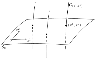
Figure 1: The surface $\mathcal{S}_{0}$ and the orbits of $G$. The orbits are depicted as curves though they are actually two-dimensional. Each orbit has only one intersection with $\mathcal{S}_{0}$.

Next, we consider the action of an element $g$ of $G$ on the points of $\mathcal{S}_{0}$. Since $G$ does not admit fixed points, each point on $\mathcal{S}_{0}$ is necessarily moved along its orbit except in the case that $g$ is the identity element $e$ of $G$. The moved points form a new surface which does not intersect with $\mathcal{S}_{0}$. We denote this surface by $\mathcal{S}_{g}$ and consider a family of the surfaces $\{\mathcal{S}_{g}\}:=\{\mathcal{S}_{g}|g\in G\}$ where $\mathcal{S}_{e}=\mathcal{S}_{0}$. It is clear that the surfaces of $\{\mathcal{S}_{g}\}$ fill the spacetime without intersecting with each other.

Let us now choose an orbit, which we denote by $\mathcal{O}_{0}$. All the surfaces of $\{\mathcal{S}_{g}\}$ cross the orbit $\mathcal{O}_{0}$ at different points, and hence the surfaces are specified by the intersections on $\mathcal{O}_{0}$. Let $(y^{1},y^{2})$ be an internal coordinate system of $\mathcal{O}_{0}$. We can denote by $\mathcal{S}_{(y^{1},y^{2})}$ the surface which intersects with $\mathcal{O}_{0}$ at $(y^{1},y^{2})$ (see Fig. 2).

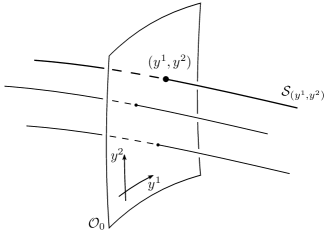
Figure 2: The orbit $\mathcal{O}_{0}$ and the surfaces of $\{\mathcal{S}_{g}\}$. Two-dimensional surfaces are depicted as curves.

Now that we have two different ways of filling ${\mathcal{M}}$: one is with the orbits of $\{\mathcal{O}_{(x^{1},x^{2})}\}$ and the other is with the surfaces of $\{\mathcal{S}_{(y^{1},y^{2})}\}$, we can specify a point of ${\mathcal{M}}$ by the orbit $\mathcal{O}_{(x^{1},x^{2})}$ and the surface $\mathcal{S}_{(y^{1},y^{2})}$ on which the point lies. Using the parameters of the orbit and the surface, we can assign the coordinates $(x^{1},x^{2},y^{1},y^{2})$ to the point. This coordinate system is convenient for studying the EOM of cohomogeneity one membranes.

II.1.2 Metric

To describe the metric, let us introduce an invariant dual basis on each orbit, which is possible when the group action of $G$ on the orbits is simply transitive. Let $\{\chi^{1},\chi^{2}\}$ be an invariant dual basis on $\mathcal{O}_{0}$, which satisfy

$$\mathcal{L}_{\boldsymbol{\xi}_{I}}\chi^{J}=0,~{}~{}(I,J=1,2)$$ (2)

where $\mathcal{L}_{\boldsymbol{\xi}}$ represents the Lie derivative along a vector field $\boldsymbol{\xi}$. With respect to the coordinate system $(y^{1},y^{2})$ on $\mathcal{O}_{0}$, $\chi^{I}$ is written as

$$\chi^{I}=\chi^{I}{}_{i}(y^{1},y^{2})\,dy^{i}.$$ (3)

Considering $y^{1}$ and $y^{2}$ as the spacetime coordinates, we can extend $\chi^{I}$ to 1-forms in ${\mathcal{M}}$ satisfying Eq. (2).

Using the invariant dual basis $\{\chi^{1},\chi^{2}\}$, we can write the spacetime metric as

$$ds^{2}=g_{pq}dx^{p}dx^{q}+2g_{pI}dx^{p}\chi^{I}+g_{I\!J}\chi^{I}\chi^{J}.$$ (4)

Here, $g_{pq},g_{pI}$ and $g_{I\!J}$ are functions of $x^{1}$ and $x^{2}$ only, which is due to the Killing equations

$$\mathcal{L}_{\boldsymbol{\xi}_{I}}g=0,$$ (5)

and Eq. (2). For later convenience, we write the metric as follows:

$$ds^{2}=h_{pq}dx^{p}dx^{q}+g_{I\!J}(\chi^{I}+N^{I}{}_{p}dx^{p})(\chi^{J}+N^{J}{}_{q}dx^{q}),$$ (6)

where

$$g_{I\!J}N^{J}{}_{p}=g_{Ip},$$ (7)

$$h_{pq}=g_{pq}-g_{I\!J}N^{I}{}_{p}N^{J}{}_{q}.$$ (8)

II.1.3 Equations of motion

When we identify the orbits with the points on $\mathcal{S}_{0}$, the world-volume $\Sigma$ is reduced to a curve on $\mathcal{S}_{0}$. We denote this curve by ${\mathcal{C}}_{0}(\lambda)$:

$${\mathcal{C}}_{0}:\mathbb{R}\ni\lambda\mapsto(x^{1}(\lambda),x^{2}(\lambda))\in\mathcal{S}_{0}.$$ (9)

Then we can label the foliating orbits with the parameter $\lambda$:

$$\mathcal{O}_{\lambda}:=\mathcal{O}_{(x^{1}(\lambda),x^{2}(\lambda))}.~{}~{}(\text{see Fig.~{}\ref{fig:C_0}})$$ (10)

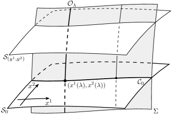
Figure 3: The curve ${\mathcal{C}}_{0}$ on the surface $\mathcal{S}_{0}$ and the orbits $\mathcal{O}_{\lambda}$ determine the world-volume $\Sigma$. The dimensions of $\Sigma$ is three, and of $\mathcal{O}_{\lambda}$ is two.

A point on $\Sigma$ is specified by the orbit $\mathcal{O}_{\lambda}$ and the surface $\mathcal{S}_{(y^{1},y^{2})}$ on which the point lies. Then the set of parameters $(\lambda,\,y^{1},y^{2})$ is considered as a coordinate system on $\Sigma$. With this coordinate system, the embedding of $\Sigma$ into ${\mathcal{M}}$ is given by

$$(\lambda,\,y^{1},y^{2})\mapsto(x^{1}(\lambda),x^{2}(\lambda),y^{1},y^{2}),$$ (11)

and the Nambu-Goto action is given by the three-volume integral

$$S=\int_{\Sigma}\!\!\sqrt{|\gamma|}\,\,d\lambda\,dy^{1}dy^{2}=\int_{{\mathcal{C}}_{0}}\!\left\{\int_{\mathcal{O}_{\lambda}}\!\!\sqrt{|\gamma|}\,\,dy^{1}dy^{2}\right\}d\lambda$$ (12)

where $\gamma$ is the determinant of the induced metric on $\Sigma$, and hence $\sqrt{|\gamma|}$ is the volume of the parallelepiped spanned by the coordinate basis $(\partial_{\lambda},\partial_{1},\partial_{2}):=(\partial/\partial\lambda,\partial/\partial y^{1},\partial/\partial y^{2})$.

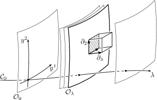
Figure 4: The parallelepiped spanned by the coordinate basis: $(\partial_{\lambda},\partial_{1},\partial_{2})$. The shaded parallelogram is spanned by $\partial_{1}$ and $\partial_{2}$. We should note that $\partial_{\lambda}$ is not necessarily perpendicular to the parallelogram.

The volume of the parallelepiped is given by a product of the area of the base and the height from the base. Considering the parallelogram spanned by $\partial_{1}$ and $\partial_{2}$ as the base (see Fig. 4), we obtain the area of the base as

$$\bigl{|}\det\chi^{I}{}_{j}\bigr{|}\sqrt{\bigl{|}\det g_{I\!J}\bigr{|}},$$ (13)

and the height of the parallelepiped, which is given by the magnitude of the normal component of $\partial_{\lambda}=\dot{x}^{p}\partial/\partial x^{p}$ to the base as

$$\sqrt{\bigl{|}h_{pq}\,\dot{x}^{p}\,\dot{x}^{q}\bigr{|}},$$ (14)

where the dot denotes the derivative with respect to $\lambda$. Thereby the volume is written as

$$\sqrt{|\gamma|}=\bigl{|}\det\chi^{I}{}_{j}\bigr{|}\sqrt{\bigl{|}\det g_{I\!J}\bigr{|}}\sqrt{\bigl{|}h_{pq}\,\dot{x}^{p}\,\dot{x}^{q}\bigr{|}}=\bigl{|}\det\chi^{I}{}_{j}\bigr{|}\sqrt{\bigl{|}(\det g_{I\!J})\,h_{pq}\,\dot{x}^{p}\,\dot{x}^{q}\bigr{|}}.$$ (15)

Noting that $\chi^{I}{}_{j}$ are functions of $y^{1}$ and $y^{2}$ and that $g_{I\!J}$ and $h_{pq}$ are functions of $\lambda$, we can write the Nambu-Goto action (12) as

$$S =\int_{{\mathcal{C}}_{0}}\left\{\sqrt{\bigl{|}(\det g_{I\!J})\,h_{pq}\,\dot{x}^{p}\,\dot{x}^{q}\bigr{|}}\int_{\mathcal{O}_{\lambda}}\!\!\bigl{|}\det\chi^{I}{}_{j}\bigr{|}\,dy^{1}dy^{2}\right\}d\lambda$$ (16)

$$=\int_{\mathcal{O}}\,\bigl{|}\det\chi^{I}{}_{j}\bigr{|}\,dy^{1}dy^{2}\int_{{\mathcal{C}}_{0}}\!\!\sqrt{\bigl{|}(\det g_{I\!J})\,h_{pq}\,\dot{x}^{p}\,\dot{x}^{q}\bigr{|}}\,d\lambda.$$ (17)

Here, we have used the fact that the integration over the orbit $\mathcal{O}_{\lambda}$ does not depend on $\lambda$. Integrating out the variables $y^{1}$ and $y^{2}$, we can reduce the Nambu-Goto action as follows:

$$S\propto\int_{{\mathcal{C}}_{0}}\!\!\sqrt{\bigl{|}(\det g_{I\!J})\,h_{pq}\,\dot{x}^{p}\,\dot{x}^{q}\bigr{|}}\,d\lambda.$$ (18)

This is identical to the action of a particle moving on the surface $\mathcal{S}_{0}$ with the metric $(\det g_{I\!J})h_{pq}$. The original problem has therefore been reduced to that of finding a geodesic on $\mathcal{S}_{0}$.

We have derived the equations of motion on the surface $\mathcal{S}_{0}$. It is also possible to do so on other surfaces of $\{\mathcal{S}_{g}\}$. The surfaces can be mapped to each other by the action of $g$ (or $g^{-1}$) and lead to the same form of (18). The reductions on the surfaces of $\{\mathcal{S}_{g}\}$ are put together by identifying the surfaces with the orbit space ${\mathcal{M}}/G$ by

$$\mathcal{S}_{g}\ni(x^{1},x^{2})\leftrightarrow\mathcal{O}_{(x^{1},x^{2})}\in{\mathcal{M}}/G.$$ (19)

We can then conclude that the equations of motions are reduced to the geodesic equations on ${\mathcal{M}}/G$. If we consider $(x^{1},x^{2})$ be a coordinate system of ${\mathcal{M}}/G$, the projection map $\pi:{\mathcal{M}}\to{\mathcal{M}}/G$ is explicitly given as

$$\pi:{\mathcal{M}}\ni(x^{1},x^{2},y^{1},y^{2})\mapsto(x^{1},x^{2})\in{\mathcal{M}}/G.$$ (20)

Let $(x^{1}(\lambda),x^{2}(\lambda))$ be a geodesic in ${\mathcal{M}}/G$. The solution of the membrane is given as a preimage: $\pi^{-1}(x^{1}(\lambda),x^{2}(\lambda))=(x^{1}(\lambda),x^{2}(\lambda),\,y^{1},\,y^{2})$. By the use of the projection $\pi$, we can naturally induce a metric on ${\mathcal{M}}/G$ in order that $\pi$ is a Riemannian submersion. Such an induced metric is given as the symmetric tensor $h_{pq}$ of (8). Weighting $h_{pq}$ with $\det g_{IJ}$, we obtain the metric used in the geodesic action (18) for the cohomogeneity one membrane.

II.2 The case $\boldsymbol{\dim G=3}$

In the case $\dim G=3$, the orbits are two-dimensional spaces of constant curvature. The metric of the orbit with constant curvature $K$ can be written in the form:

$$d\sigma^{2}=R^{2}\Bigl{\{}(dy^{1})^{2}+\epsilon\,F^{2}(y^{1})\,(dy^{2})^{2}\Bigr{\}}$$ (21)

with

$$\epsilon:=\begin{cases}+1&\text{(spacelike orbits)}\\ -1&\text{(timelike orbits)}\end{cases}$$ (22)

and

$$F(y^{1}):=\begin{cases}\sin y^{1}&(K>0)\\ y^{1}&(K=0)\\ \sinh y^{1}&(K<0)\end{cases},$$ (23)

where $R$ is a constant. By using coordinates $x^{1}$ and $x^{2}$ which are constant on each orbit, we can write the spacetime metric as P34_Goenner:1970 ; P34_ExactSolution :

$$ds^{2}=e^{2\lambda}(dx^{1})^{2}-\epsilon e^{2\nu}(dx^{2})^{2}+R^{2}\Bigl{\{}(dy^{1})^{2}+\epsilon F^{2}(y^{1})(dy^{2})^{2}\Bigr{\}},$$ (24)

where $\lambda,\nu$ and $R$ are functions of $x^{1}$ and $x^{2}$. We can consider $(x^{1},x^{2})$ as a coordinate system of the orbit space ${\mathcal{M}}/G$ and the projection $\pi:{\mathcal{M}}\to{\mathcal{M}}/G$ is again given by Eq. (20). We see that

$$ds_{{\mathcal{M}}/G}^{2}:=e^{2\lambda}(dx^{1})^{2}-\epsilon e^{2\nu}(dx^{2})^{2}$$ (25)

is the metric on ${\mathcal{M}}/G$ with $\pi$ being a Riemannian submersion. Following the same derivation presented in the case $\dim G=2$, the Nambu-Goto action is separated as

$$S=\int_{\mathcal{O}}\bigl{|}\Sigma\bigr{|}\,dy^{1}dy^{2}\,\int_{{\mathcal{C}}}\sqrt{\left|R^{4}\Bigl{\{}e^{2\lambda}(\dot{x}^{1})^{2}-\epsilon e^{2\nu}(\dot{x}^{2})^{2}\Bigr{\}}\right|}\,d\lambda.$$ (26)

Integrating out the variables $y^{1}$ and $y^{2}$, we obtain a reduced action

$$S\propto\int_{{\mathcal{C}}}\sqrt{\left|R^{4}\Bigl{\{}e^{2\lambda}(\dot{x}^{1})^{2}-\epsilon e^{2\nu}(\dot{x}^{2})^{2}\Bigr{\}}\right|}\,d\lambda.$$ (27)

Therefore the problem is reduced to solving the geodesic equations on ${\mathcal{M}}/G$ with the weighted metric

$$\widetilde{ds}_{{\mathcal{M}}/G}^{2}:=R^{4}\,ds_{{\mathcal{M}}/G}^{2}=R^{4}\Bigl{\{}e^{2\lambda}(dx^{1})^{2}-\epsilon e^{2\nu}(dx^{2})^{2}\Bigr{\}}.$$ (28)

We finally note the Lie algebra ${\mathfrak{g}}$ of $G$. In the case $\dim G=3$, the action of $G$ is described by three Killing vector fields, $\boldsymbol{\xi}_{I}~{}(I=1,2,3)$. The triple $(\boldsymbol{\xi}_{1},\,\boldsymbol{\xi}_{2},\,\boldsymbol{\xi}_{3})$ represents a basis of ${\mathfrak{g}}$. The commutation relations are those of the two-dimensional spaces of constant curvature, which are listed in Table 1 in terms of the Bianchi classification of the three-dimensional Lie algebras. As seen in Table 1, the Lie algebras of Bianchi $\text{VI}_{\text{0}}$ and $\text{VII}_{\text{0}}$ have two-dimensional commutative subalgebras spanned by $\boldsymbol{\xi}_{1}$ and $\boldsymbol{\xi}_{2}$. As for the Bianchi VIII, taking new bases

$$\boldsymbol{\xi}^{\prime}_{1}:=\boldsymbol{\xi}_{2}-\boldsymbol{\xi}_{3},~{}~{}\boldsymbol{\xi}^{\prime}_{2}:=\boldsymbol{\xi}_{1},$$ (29)

which satisfy

$$[\boldsymbol{\xi}^{\prime}_{1},\,\boldsymbol{\xi}^{\prime}_{2}]=\boldsymbol{\xi}^{\prime}_{1},$$ (30)

we find that the Bianchi VIII also have a two-dimensional solvable subalgebra. Since the Lie algebras of Bianchi $\text{VI}_{\text{0}}$, $\text{VII}_{\text{0}}$ and VIII include two-dimensional subalgebras, the groups associated with these Lie algebras include two-dimensional subgroups, whose actions on the orbits are simply transitive. Then, for the groups of Bianchi $\text{VI}_{\text{0}}$, $\text{VII}_{\text{0}}$ and VIII, the reduction of the EOM can be explained in the case $\dim G=2$.

spaces of constant curvature	Bianchi type	$[\boldsymbol{\xi}_{1},\,\boldsymbol{\xi}_{2}]$	$[\boldsymbol{\xi}_{2},\,\boldsymbol{\xi}_{3}]$	$[\boldsymbol{\xi}_{3},\,\boldsymbol{\xi}_{1}]$
Euclid space $E^{2}$	$\text{VII}_{\text{0}}$	$0$	$-\boldsymbol{\xi}_{1}$	$-\boldsymbol{\xi}_{2}$
sphere $S^{2}$	IX	$-\boldsymbol{\xi}_{3}$	$-\boldsymbol{\xi}_{1}$	$-\boldsymbol{\xi}_{2}$
hyperbolic space $H^{2}$	VIII	$\boldsymbol{\xi}_{3}$	$-\boldsymbol{\xi}_{1}$	$-\boldsymbol{\xi}_{2}$
Minkowski spacetime $E^{1,1}$	$\text{VI}_{\text{0}}$	$0$	$\boldsymbol{\xi}_{1}$	$-\boldsymbol{\xi}_{2}$
de Sitter spacetime $dS^{2}$	VIII	$\boldsymbol{\xi}_{3}$	$-\boldsymbol{\xi}_{1}$	$-\boldsymbol{\xi}_{2}$
anti-de Sitter spacetime $AdS^{2}$	VIII	$\boldsymbol{\xi}_{3}$	$-\boldsymbol{\xi}_{1}$	$-\boldsymbol{\xi}_{2}$

Table 1: The commutation relations of three Killing vectors $(\boldsymbol{\xi}_{1},\,\boldsymbol{\xi}_{2},\,\boldsymbol{\xi}_{3})$ of the two-dimensional spaces of constant curvature.

III General classification method for cohomogeneity one membranes

The cohomogeneity one symmetries can be assumed in the spacetimes whose isometry groups admit subgroups $G$ with two-dimensional orbits. In a given such spacetime, different $G$ may give the cohomogeneity one membranes which are essentially the same. To discard such redundancy, we shall introduce the notion of geometrical equivalence of world-volumes and present the method of classifying cohomogeneity one membranes up to the equivalence.

Let $\Sigma$ and $\Sigma^{\prime}$ be world-volumes. We say that they are geometrically equivalent if there is an isometry $\phi$ on ${{\mathcal{M}}}$ which maps $\Sigma$ onto $\Sigma^{\prime}$. Suppose further that one of such world-volumes, $\Sigma$, is of cohomogeneity one with symmetry group $G$. Then $\Sigma^{\prime}$ is of cohomogeneity one with symmetry group $\phi G\phi^{-1}$. To see this, let $\mathcal{O}_{\lambda}$ be the orbits of $G$ which comprise a foliation of $\Sigma$. Then for each pair of points $p$ and $p^{\prime}$ on $\phi(\mathcal{O}_{\lambda})$, there exists $g\in G$ such that $g(\phi^{-1}(p))=\phi^{-1}(p^{\prime})$ which implies $\phi g\phi^{-1}(p)=p^{\prime}$. Thus $\phi(\mathcal{O}_{\lambda})$ comprise a homogeneous foliation of $\Sigma^{\prime}$ with symmetry group $\phi G\phi^{-1}$.

It is natural to introduce an equivalence relation for subgroups $G$ and $G^{\prime}$ of $\operatorname{Isom}{\mathcal{M}}$:

$$G\sim G^{\prime}\Leftrightarrow{}^{\exists}\phi\in\mathrm{Isom}\,{\mathcal{M}}~{}~{}\text{s.t.}~{}G^{\prime}=\phi G\phi^{-1}.$$ (31)

Then subgroups $G$ and $G^{\prime}$ define geometrically equivalent world-volumes if and only if they are equivalent. Our task is to find out the equivalence classes of the relation (31), or the conjugacy class of the subgroups $G$ of $\operatorname{Isom}{\mathcal{M}}$.

In the actual classification procedure, it is more convenient to work with the Lie algebra ${\mathfrak{g}}$ of $G$, which consists of Killing vector fields on ${\mathcal{M}}$. Because the conjugation for $g\in G$ by $\phi\in\operatorname{Isom}{\mathcal{M}}$, $g\mapsto\phi g\phi^{-1}$, induces the pushforward $\boldsymbol{\xi}\mapsto{\phi}_{\ast}{\boldsymbol{\xi}}$ for $\boldsymbol{\xi}\in{\mathfrak{g}}$. The equivalence relation on the symmetry group $G$ induces that on the symmetry Lie algebra ${\mathfrak{g}}$:

$${\mathfrak{g}}\sim{\mathfrak{g}}^{\prime}\Leftrightarrow{}^{\exists}\phi\in\mathrm{Isom}\,{\mathcal{M}}~{}~{}\text{s.t.}~{}{\mathfrak{g}}^{\prime}=\phi_{*}{\mathfrak{g}}.$$ (32)

Thus we shall classify the Lie subalgebras ${\mathfrak{g}}$ of the Lie algebra of $\operatorname{Isom}{\mathcal{M}}$, up to the equivalence relation (32).

We further would like to derive a basis for each classified symmetry Lie algebra ${\mathfrak{g}}$, so that it is convenient in applications. Let $V:=(\boldsymbol{\xi}_{1},...,\boldsymbol{\xi}_{\dim G})$ a basis for a symmetry algebra ${\mathfrak{g}}$. The bases $V$ and $V^{\prime}:=(\boldsymbol{\xi}^{\prime}_{1},...,\boldsymbol{\xi}^{\prime}_{\dim G})$ give the same ${\mathfrak{g}}$ when each element of $V^{\prime}$ is a linear combination of the elements of $V$: $\boldsymbol{\xi}^{\prime}_{i}={A_{i}}^{j}\boldsymbol{\xi}_{j}$, $A_{i}{}^{j}\in\text{GL}(\dim G,\mathbb{R})$. Then the classification of all cohomogeneity one membrane in a given spacetime ${\mathcal{M}}$ reduces to that of the bases for the symmetry algebras under the equivalence relation

$$V\sim V^{\prime}\Leftrightarrow{}^{\exists}\phi\in\mathrm{Isom}\,{\mathcal{M}},{}^{\exists}{A_{i}}^{j}\in\text{GL}(\dim G,\mathbb{R})~{}~{}\text{s.t.}~{}\boldsymbol{\xi}^{\prime}_{i}={A_{i}}^{j}{\phi}_{\ast}\boldsymbol{\xi}_{j}.$$ (33)

A concrete procedure to get a set of class representatives is the following.

Step 1. Choose an abstract Lie algebra ${\mathfrak{g}}$ of the symmetry group $G$. It must be one of the following six:

$$\text{$\mathbb{R}^{2}$, two-dimensional non-commutative algebra},$$

$$\text{Bianchi types {$\text{VI}_{\text{0}}$}, {$\text{VII}_{\text{0}}$}, {$\text{VIII}$} and {$\text{IX}$}}.$$ (34)

As discussed in Sec. II, the above are the only Lie algebras that allow two-dimensional orbits. Furthermore, as mentioned at the end of Sec. II, one can eliminate Bianchi types $\text{VI}_{\text{0}}$, $\text{VII}_{\text{0}}$ and VIII from the list (34), because they are the special cases of $\mathbb{R}^{2}$ and two-dimensional non-commutative algebra. However, here we retain them so as to include all possible cases that the orbits are spaces of constant curvature and the metric on the orbit space has the simple form (28).

Step 2. Find a general set of Killing vector fields on ${\mathcal{M}}$, $V=(\boldsymbol{\xi}_{1},...,\boldsymbol{\xi}_{\dim G})$, that satisfy one of the commutation relations (1) and those in Table 1 depending on the Lie algebra chosen in Step 1. Check that the orbit of $V$ is two-dimensional.

Step 3-$k$ ($k=1,...,\dim G$). Canonicalize $\boldsymbol{\xi}_{k}$. Namely, reduce $\boldsymbol{\xi}_{k}$ to a certain simple form by using the degrees of freedom of the equivalence relation (33) that preserves $\boldsymbol{\xi}_{l}$ for $l<k$. We shall say that such $(\boldsymbol{\xi}_{1},...,\boldsymbol{\xi}_{k})$ has the canonical form. [We might sometimes rearrange the canonical form $(\boldsymbol{\xi}_{1},...,\boldsymbol{\xi}_{k})$ by using $\text{GL}(k,\mathbb{R})$ in order to make it look simpler as a whole.] Finally, with $k=\dim G$, we obtain the canonical form of $V$.

IV Classification in Minkowski spacetime

We have obtained the general scheme to classify cohomogeneity one membranes in a given spacetime. In this section, we carry out the complete classification in Minkowski spacetime, which admits ten linearly independent Killing vectors,

$$\begin{array}[]{rll}\boldsymbol{P}\kern-1.0pt_{\mu}&~{}~{}\kern-3.00003pt(\mu=t,\,x,\,y,\,z),&~{}~{}\text{Translations};\\ \boldsymbol{K}\kern-1.0pt_{i}&~{}~{}\kern-3.00003pt(i=x,\,y,\,z),&~{}~{}\text{Lorentz boosts};\\ \boldsymbol{L}_{i}&~{}~{}\kern-3.00003pt(i=x,\,y,\,z),&~{}~{}\text{Rotations}.\end{array}$$ (35)

Any Killing vector $\boldsymbol{\xi}$ is written as a linear combination of them,

$$\boldsymbol{\xi}=\alpha_{\mu}\boldsymbol{P}\kern-1.0pt_{\mu}+\beta_{i}\boldsymbol{K}\kern-1.0pt_{i}+\gamma_{i}\boldsymbol{L}_{i},$$ (36)

where $\alpha_{\mu}$, $\beta_{i}$ and $\gamma_{i}$ are constants.

In Minkowski spacetime, we have an advantage that greatly simplifies the classification scheme because all canonical forms of Killing vector fields are derived P34_Ishihara:2005nu . For any ${\mathfrak{g}}$, we can assume that $\boldsymbol{\xi}_{1}$ is one of the canonical forms listed in Table 2 up to scalar multiplication. Thus Step 3-1 is essentially done in advance.

Type	Canonical form
I	$a\boldsymbol{P}\kern-1.0pt_{t}+b\boldsymbol{L}_{z}$
II	$a(\boldsymbol{P}\kern-1.0pt_{t}+\boldsymbol{P}\kern-1.0pt_{z})+b\boldsymbol{L}_{z}$
III	$a\boldsymbol{P}\kern-1.0pt_{z}+b\boldsymbol{L}_{z}$
IV	$a\boldsymbol{P}\kern-1.0pt_{z}+b(\boldsymbol{K}\kern-1.0pt_{y}+\boldsymbol{L}_{z})$
V	$a\boldsymbol{P}\kern-1.0pt_{z}+b\boldsymbol{K}\kern-1.0pt_{y}$
VI	$a\boldsymbol{P}\kern-1.0pt_{x}+b(\boldsymbol{K}\kern-1.0pt_{y}+\boldsymbol{L}_{z})$
VII	$a\boldsymbol{K}\kern-1.0pt_{z}+b\boldsymbol{L}_{z}$
	($a$, $b$: constants)

Table 2: Canonical forms of the Killing vectors in Minkowski spacetime. Any Killing vectors are transformed by isometries to these seven types. Killing vectors in the same canonical form with different pairs of constants $(a,b)$ cannot be transformed to each other.

IV.1 Classification of two-dimensional Abelian symmetry groups

Let us choose the two-dimensional commutative algebra $\mathbb{R}^{2}$ as the symmetry algebra ${\mathfrak{g}}$. We would like to derive the equivalence classes of the set of commuting pairs of Killing vector fields,

$${\cal V}_{\mathrm{C}}:=\left\{(\boldsymbol{\xi}_{1},\,\boldsymbol{\xi}_{2})\,|\,[\boldsymbol{\xi}_{1},\,\boldsymbol{\xi}_{2}]=0\right\}.$$ (37)

As discussed above, Step 3-1 is already carried out and we can take $\boldsymbol{\xi}_{1}$ as one of the canonical forms of Table 2 up to scalar multiplication. We then divide ${\cal V}_{\mathrm{C}}$ essentially into seven parts ${\cal V}_{\mathrm{C}}^{J}~{}~{}(J=\mathrm{I},~{}\mathrm{II},\dots,\mathrm{VII}$) depending on the canonical form of $\boldsymbol{\xi}_{1}$. For example, ${\cal V}_{\mathrm{C}}^{\mathrm{I}}$ is a set of the commuting pairs of Killing vectors $(\boldsymbol{\xi}_{1},\,\boldsymbol{\xi}_{2})$ with $\boldsymbol{\xi}_{1}$ being in the canonical form of Type I, $\boldsymbol{\xi}_{1}=a\boldsymbol{P}\kern-1.0pt_{t}+b\boldsymbol{L}_{z}$, and in this case $\boldsymbol{\xi}_{2}$ is written as linear combinations of the ten Killing vectors (35) which commute with $a\boldsymbol{P}\kern-1.0pt_{t}+b\boldsymbol{L}_{z}$. Next, we reduce the number of the Killing vectors (35) contained in $\boldsymbol{\xi}_{1}$ and $\boldsymbol{\xi}_{2}$ by using isometries and $\text{GL}(2,\mathbb{R})$ actions on the pair $(\boldsymbol{\xi}_{1},\,\boldsymbol{\xi}_{2})$, so that $\boldsymbol{\xi}_{1}$ and $\boldsymbol{\xi}_{2}$ contains the smallest possible number of parameters. A detailed calculation for one case is given in Appendix.

As a result, we obtain simple representatives in each of ${\cal V}_{\mathrm{C}}^{J}$. However, we must be aware that two different ${\cal V}_{\mathrm{C}}^{J}$’s may lead to equivalent pairs $(\boldsymbol{\xi}_{1},\boldsymbol{\xi}_{2})$. We eliminate this redundancy and obtain a complete set of canonical forms. The result is shown in Table 3. Any element of ${\cal V}_{\mathrm{C}}$ falls into one of the equivalence classes of these canonical forms.

$\boldsymbol{\xi}_{1}$	$\boldsymbol{\xi}_{2}$   ($a$, $b$: constants)
$\boldsymbol{P}\kern-1.0pt_{t}$	$a\boldsymbol{P}\kern-1.0pt_{z}+b\boldsymbol{L}_{z}$
$\boldsymbol{P}\kern-1.0pt_{t}+\boldsymbol{P}\kern-1.0pt_{z}$	$a\boldsymbol{P}\kern-1.0pt_{t}+b\boldsymbol{L}_{z}$,  $a\boldsymbol{P}\kern-1.0pt_{z}+b(\boldsymbol{K}\kern-1.0pt_{x}-\boldsymbol{L}_{y})$,  $a\boldsymbol{P}\kern-1.0pt_{y}+b(\boldsymbol{K}\kern-1.0pt_{x}-\boldsymbol{L}_{y})$
$\boldsymbol{P}\kern-1.0pt_{z}$	$a\boldsymbol{P}\kern-1.0pt_{t}+b\boldsymbol{L}_{z}$,  $a\boldsymbol{P}\kern-1.0pt_{x}+b\boldsymbol{K}\kern-1.0pt_{y}$,  $a\boldsymbol{P}\kern-1.0pt_{x}+b(\boldsymbol{K}\kern-1.0pt_{y}+\boldsymbol{L}_{z})$
$\boldsymbol{L}_{z}$	$\boldsymbol{K}\kern-1.0pt_{z}$
$\boldsymbol{K}\kern-1.0pt_{y}+\boldsymbol{L}_{z}$	$a\boldsymbol{P}\kern-1.0pt_{z}+b(\boldsymbol{K}\kern-1.0pt_{z}-\boldsymbol{L}_{y})$

Table 3: The representatives of the equivalence classes of ${\cal V}_{\mathrm{C}}$: a set of commuting pairs of Killing vectors $(\boldsymbol{\xi}_{1},\,\boldsymbol{\xi}_{2})$. Those pairs that are connected by a simple rescaling of $\boldsymbol{\xi}_{2}$ are equivalent, though having different $(a,b)$.

IV.2 Classification of two-dimensional non-Abelian symmetry groups

Let us choose the two-dimensional non-commutative algebra as the symmetry algebra ${\mathfrak{g}}$. This is the classification of ${\cal V}_{\mathrm{S}}:=\left\{(\boldsymbol{\xi}_{1},\,\boldsymbol{\xi}_{2})\,|\,[\boldsymbol{\xi}_{1},\,\boldsymbol{\xi}_{2}]=\boldsymbol{\xi}_{1}\right\}$. As in the commutative case, we can take $\boldsymbol{\xi}_{1}$ to be the seven types in Table 2 and we reduce the degree of freedom in ${\cal V}_{\mathrm{S}}$ by using $\phi\in\operatorname{Isom}{\mathcal{M}}$ and $A_{i}{}^{j}\in\text{GL}(2,\mathbb{R})$ which preserves the commutation relation. The resulting canonical forms are listed in Table 4.

$\boldsymbol{\xi}_{1}$	$\phantom{-}\boldsymbol{\xi}_{2}$   ($a$: constant)
$\boldsymbol{P}\kern-1.0pt_{t}+\boldsymbol{P}\kern-1.0pt_{z}$	$\phantom{-}\boldsymbol{K}\kern-1.0pt_{z}+a\boldsymbol{P}\kern-1.0pt_{x}$, $\boldsymbol{K}\kern-1.0pt_{z}+a\boldsymbol{L}_{z}$
$\boldsymbol{K}\kern-1.0pt_{y}+\boldsymbol{L}_{z}$	$-\boldsymbol{K}\kern-1.0pt_{x}+a\boldsymbol{P}\kern-1.0pt_{z}$

Table 4: The representatives of the equivalence classes of ${\cal V}_{\mathrm{S}}$: a set of non-commuting pairs of Killing vectors $(\boldsymbol{\xi}_{1},\,\boldsymbol{\xi}_{2})$.

IV.3 Classification of three-dimensional symmetry groups

Let us discuss the case that the symmetry algebra ${\mathfrak{g}}$ is three-dimensional. As was discussed in the previous section, ${\mathfrak{g}}$ must be one of the Bianchi types $\text{VI}_{\text{0}}$, $\text{VII}_{\text{0}}$, VIII and IX. The classification is for the triples of Killing vector fields $(\boldsymbol{\xi}_{1},\boldsymbol{\xi}_{2},\boldsymbol{\xi}_{3})$ which satisfy either of the commutation relations listed in Table 1. The classification procedure for each Bianchi type is described in the subsequent subsections. The result of the canonical forms for all Bianchi types are shown in Table 5.

Bianchi type	$\boldsymbol{\xi}_{1}$	$\boldsymbol{\xi}_{2}$	$\boldsymbol{\xi}_{3}$
$\text{VI}_{\text{0}}$	$\boldsymbol{P}\kern-1.0pt_{t}$	$\boldsymbol{P}\kern-1.0pt_{z}$	$\boldsymbol{K}\kern-1.0pt_{z}$
$\text{VII}_{\text{0}}$	$\boldsymbol{P}\kern-1.0pt_{z}$	$\boldsymbol{P}\kern-1.0pt_{x}$	$\boldsymbol{L}_{y}$
	$\boldsymbol{K}\kern-1.0pt_{y}+\boldsymbol{L}_{z}$	$\boldsymbol{K}\kern-1.0pt_{z}-\boldsymbol{L}_{y}$	$\boldsymbol{L}_{x}$
VIII	$\boldsymbol{K}\kern-1.0pt_{z}$	$\boldsymbol{K}\kern-1.0pt_{x}$	$\boldsymbol{L}_{y}$
IX	$\boldsymbol{L}_{z}$	$\boldsymbol{L}_{x}$	$\boldsymbol{L}_{y}$

Table 5: The representatives of the equivalence classes of triples of Killing vectors $(\boldsymbol{\xi}_{1},\,\boldsymbol{\xi}_{2},\,\boldsymbol{\xi}_{3})$ that generate isometry group that has two-dimensional orbits.

IV.3.1 Bianchi $\text{VI}_{\text{0}}$

Bianchi type $\text{VI}_{\text{0}}$ algebra has a two-dimensional commutative subalgebra ${\mathfrak{h}}$. The subalgebra ${\mathfrak{h}}$ must be equivalent to one of the Lie algebras defined by the pairs in Table 3. Then we should look for the third Killing vector $\boldsymbol{\xi}_{3}$ which satisfies the commutation relations

$$[\boldsymbol{\xi}_{2},\,\boldsymbol{\xi}_{3}]=\boldsymbol{\xi}_{1},\ [\boldsymbol{\xi}_{3},\,\boldsymbol{\xi}_{1}]=-\boldsymbol{\xi}_{2}.$$ (38)

where we take a linear combinations $\boldsymbol{\xi}_{i}$ if necessary. Reducing the general expression of $V=(\boldsymbol{\xi}_{1},\,\boldsymbol{\xi}_{2},\,\boldsymbol{\xi}_{3})$ by using the equivalence relation (33) leads to the canonical form

$$V=(\boldsymbol{P}\kern-1.0pt_{t},\,\boldsymbol{P}\kern-1.0pt_{z},\,\boldsymbol{K}\kern-1.0pt_{z}+\alpha_{\mu}\boldsymbol{P}\kern-1.0pt_{\mu}+\gamma\boldsymbol{L}_{z}),$$ (39)

where $\alpha_{\mu}$ and $\gamma$ are arbitrary constants.

Let us require that the symmetry group $G$ have the two-dimensional orbits. The tangent space spanned by $V$ at each point must be two-dimensional. The concrete expression of the Killing vector fields,

$$\boldsymbol{\xi}_{1}=\partial_{t},\ \boldsymbol{\xi}_{2}=\partial_{z},\ \boldsymbol{\xi}_{3}=z\partial_{t}+t\partial_{z}+\alpha_{x}\partial_{x}+\alpha_{y}\partial_{y}+\gamma(x\partial_{y}-y\partial_{x}),$$ (40)

in Cartesian coordinate basis implies that $\boldsymbol{\xi}_{3}$ cannot have the terms proportional to $\partial_{x}$ or $\partial_{y}$. Thus, we must have $\alpha_{\mu}=0$ and $\gamma=0$ so that

$$V=(\boldsymbol{P}\kern-1.0pt_{t},\,\boldsymbol{P}\kern-1.0pt_{z},\,\boldsymbol{K}\kern-1.0pt_{z}).$$ (41)

The orbits of ${\mathfrak{g}}$ are obviously the planes parallel to the $t$-$z$ plane. We note that the Lie algebra spanned by the basis $V$ contains both of the commutative and non-commutative two-dimensional algebras, spanned by $(\boldsymbol{P}\kern-1.0pt_{t},\,\boldsymbol{P}\kern-1.0pt_{z})$ in Table 3 and $(\boldsymbol{P}\kern-1.0pt_{t}+\boldsymbol{P}\kern-1.0pt_{z},\,\boldsymbol{K}\kern-1.0pt_{z})$ in Table 4, respectively. Accordingly, the two-dimensional orbits of (41) can be considered as those generated by $(\boldsymbol{P}\kern-1.0pt_{t},\,\boldsymbol{P}\kern-1.0pt_{z})$ or by $(\boldsymbol{P}\kern-1.0pt_{t}+\boldsymbol{P}\kern-1.0pt_{z},\,\boldsymbol{K}\kern-1.0pt_{z})$. The orbit is the two-dimensional Minkowski spacetime.

IV.3.2 Bianchi $\text{VII}_{\text{0}}$

Let us consider the case of ${\mathfrak{g}}$ being the Bianchi $\text{VII}_{\text{0}}$ algebra. Then $\boldsymbol{\xi}_{1}$ and $\boldsymbol{\xi}_{2}$ in $V=(\boldsymbol{\xi}_{1},\,\boldsymbol{\xi}_{2},\,\boldsymbol{\xi}_{3})$ commute. Following the same procedures as in the case of Bianchi $\text{VI}_{\text{0}}$, we obtain two representatives,

$$V=(\boldsymbol{P}\kern-1.0pt_{z},\,\boldsymbol{P}\kern-1.0pt_{x},\,\boldsymbol{L}_{y})\ \text{and}\ (\boldsymbol{K}\kern-1.0pt_{y}+\boldsymbol{L}_{z},\,\boldsymbol{K}\kern-1.0pt_{z}-\boldsymbol{L}_{y},\,\boldsymbol{L}_{x}).$$ (42)

In the first case, which we call type ${\text{VII}_{\text{0}}}$–1, the orbits are parallels to the $z$-$x$ plane and are intrinsically and extrinsically flat. In contrast, in the second case, which we call type ${\text{VII}_{\text{0}}}$–2, the orbits are flat intrinsically but are embedded in ${\mathcal{M}}$ in an non-trivial way. Both types of embedding share common features: intrinsic flatness and extrinsic homogeneity and isotropy. The type ${\text{VII}_{\text{0}}}$–2 with non-trivial embedding of orbits seems worth further analysis. In Sec. V, we will clarify how the orbits of type ${\text{VII}_{\text{0}}}$–2 are embedded in Minkowski spacetime, and will explicitly construct a solution of a cohomogeneity one Nambu-Goto membrane.

IV.3.3 Bianchi VIII

Let the symmetry algebra ${\mathfrak{g}}$ be the Bianchi VIII algebra. We start with $\boldsymbol{\xi}_{1}$ of the $V=(\boldsymbol{\xi}_{1},\,\boldsymbol{\xi}_{2},\,\boldsymbol{\xi}_{3})$ being one of the canonical form in Table 2 (up to rescaling). Next, for the chosen $\boldsymbol{\xi}_{1}$, we look for $\boldsymbol{\xi}_{2}$ which satisfies following relations

$$[\boldsymbol{\xi}_{1},\,[\boldsymbol{\xi}_{1},\,\boldsymbol{\xi}_{2}]] =[\boldsymbol{\xi}_{1},\,\boldsymbol{\xi}_{3}]=\boldsymbol{\xi}_{2},$$ (43)

$$[\boldsymbol{\xi}_{2},\,[\boldsymbol{\xi}_{1},\,\boldsymbol{\xi}_{2}]] =[\boldsymbol{\xi}_{2},\,\boldsymbol{\xi}_{3}]=-\boldsymbol{\xi}_{1}.$$ (44)

The third Killing vector $\boldsymbol{\xi}_{3}$ is obtained through the commutation relation

$$\boldsymbol{\xi}_{3}=[\boldsymbol{\xi}_{1},\,\boldsymbol{\xi}_{2}].$$ (45)

We then have possible $V$. By using $\text{GL}(3,\mathbb{R})$ that preserves the commutation relations, we find that there is only one equivalence class represented by

$$V=(\boldsymbol{K}\kern-1.0pt_{x},\,\boldsymbol{K}\kern-1.0pt_{y},\,\boldsymbol{L}_{z}).$$ (46)

The orbits are two-dimensional hyperboloids or de Sitter spacetimes which are embedded in $E^{2,1}$ with the equation

$$-t^{2}+x^{2}+y^{2}=\text{const.}$$ (47)

As mentioned in subsection II.2, the Lie algebra ${\mathfrak{g}}$ spanned by $V$ includes a solvable subalgebra spanned by $(\boldsymbol{K}\kern-1.0pt_{y}+\boldsymbol{L}_{z},\,-\boldsymbol{K}\kern-1.0pt_{x})$, which is a special case in Table 4.

IV.3.4 Bianchi IX

Let ${\mathfrak{g}}$ be the Bianchi IX algebra. As in the case of Bianchi VIII, we first consider $\boldsymbol{\xi}_{1}$ to be in a canonical form in Table 2. We then look for $\boldsymbol{\xi}_{2}$ which satisfies

$$[\boldsymbol{\xi}_{1},\,[\boldsymbol{\xi}_{1},\,\boldsymbol{\xi}_{2}]] =[\boldsymbol{\xi}_{1},\,-\boldsymbol{\xi}_{3}]=-\boldsymbol{\xi}_{2},$$ (48)

$$[\boldsymbol{\xi}_{2},\,[\boldsymbol{\xi}_{1},\,\boldsymbol{\xi}_{2}]] =[\boldsymbol{\xi}_{2},\,-\boldsymbol{\xi}_{3}]=\boldsymbol{\xi}_{1}.$$ (49)

The third Killing vector $\boldsymbol{\xi}_{3}$ is obtained through the commutation relation

$$\boldsymbol{\xi}_{3}=[\boldsymbol{\xi}_{1},\,\boldsymbol{\xi}_{2}].$$ (50)

By using isometries and $\text{GL}(3,\mathbb{R})$ actions, we then find that there is only one equivalence class represented by

$$V=(\boldsymbol{\xi}_{1},\,\boldsymbol{\xi}_{2},\,\boldsymbol{\xi}_{3})=(\boldsymbol{L}_{z},\,\boldsymbol{L}_{x},\,\boldsymbol{L}_{y}).$$ (51)

The orbits are spheres centered at the origin.

V Exact solution for Type ${\text{VII}_{\text{0}}}$–2 membrane

Applying the results of subsection II.2, we solve the Nambu-Goto equations for the cohomogeneity one membrane whose world-volume has the symmetry of Bianchi type $\text{VII}_{\text{0}}$. The symmetry algebra ${\mathfrak{g}}$ has two possibilities: one is type ${\text{VII}_{\text{0}}}$–1 generated by $(\boldsymbol{P}\kern-1.0pt_{z},\,\boldsymbol{P}\kern-1.0pt_{x},\,\boldsymbol{L}_{y})$ and the other is type ${\text{VII}_{\text{0}}}$–2 generated by $(\boldsymbol{K}\kern-1.0pt_{y}+\boldsymbol{L}_{z},\,\boldsymbol{K}\kern-1.0pt_{z}-\boldsymbol{L}_{y},\,\boldsymbol{L}_{x})$,

In the case of type ${\text{VII}_{\text{0}}}$–1, the orbits are the $t=\text{const.}$ and $y=\text{const.}$ planes. The weighted metric of the orbit space, whose geodesics determine the dynamics of the membrane, is flat. Then, cohomogeneity one membrane of type ${\text{VII}_{\text{0}}}$–1 is a static plane or its equivalents.

Hereafter, we concentrate on type ${\text{VII}_{\text{0}}}$–2. We follow the same conventions as in subsection II.2: the coordinates on the orbits are denoted by $(y^{1},y^{2})$, and the orbits are distinguished by $(x^{1},x^{2})$.

V.1 Embbeding of type ${\text{VII}_{\text{0}}}$–2 orbits

We begin with clarifying the embedding of the $\text{VII}_{\text{0}}$-orbits: $\vec{y}:=(y^{1},y^{2})\mapsto(t,x,y,z)$, generated by the Killing vectors

$$(\boldsymbol{K}\kern-1.0pt_{y}+\boldsymbol{L}_{z},\,\boldsymbol{K}\kern-1.0pt_{z}-\boldsymbol{L}_{y},\,\boldsymbol{L}_{x}).$$ (52)

Since the Killing vectors $\boldsymbol{K}\kern-1.0pt_{y}+\boldsymbol{L}_{z}$ and $\boldsymbol{K}\kern-1.0pt_{z}-\boldsymbol{L}_{y}$ commute with each other, we take them as a coordinate basis on the orbit:

$$(\partial_{y^{1}},\partial_{y^{2}})=(\boldsymbol{K}\kern-1.0pt_{y}+\boldsymbol{L}_{z},\boldsymbol{K}\kern-1.0pt_{z}-\boldsymbol{L}_{y}).$$ (53)

In Cartesian coordinates $(t,x,y,z)$, Eqs. (53) are written as

$$\partial_{y^{1}} =t_{,1}\partial_{t}+x_{,1}\partial_{x}+y_{,1}\partial_{y}+z_{,1}\partial_{z}=y(\partial_{t}-\partial_{x})+(t+x)\partial_{y},$$ (54)

$$\partial_{y^{2}} =t_{,2}\partial_{t}+x_{,2}\partial_{x}+y_{,2}\partial_{y}+z_{,2}\partial_{z}=z(\partial_{t}-\partial_{x})+(t+x)\partial_{z},$$ (55)

where $t$, $x$, $y$ and $z$ are considered as embedding functions, namely functions of $y^{i}~{}(i=1,2)$, and the commas denote the differentiation with respect to $y^{i}$. Comparing the coefficients of the coordinate basis, we obtain equations of the embedding:

$$\dfrac{\partial t}{\partial y^{1}}=-\dfrac{\partial x}{\partial y^{1}}=y, \dfrac{\partial t}{\partial y^{2}}=-\dfrac{\partial x}{\partial y^{2}}=z, \dfrac{\partial y}{\partial y^{1}}=\dfrac{\partial z}{\partial y^{2}}=(t+x), \dfrac{\partial z}{\partial y^{1}}=\dfrac{\partial y}{\partial y^{2}}=0.$$ (56)

These equations are readily solved as

$$t=\dfrac{a}{2}\,\vec{y}\!\cdot\!\vec{y}+\frac{a+b}{2},~{}~{}x=-t+a,~{}~{}y=ay^{1},~{}~{}z=ay^{2},$$ (57)

where $a$ and $b$ are arbitrary constants. Eqs. (57) are equivalent to the following implicit equations

$$-\left(t-\frac{b}{2}\right)^{2}+\left(x+\frac{b}{2}\right)^{2}+y^{2}+z^{2}=0,$$ (58)

$$t+x-a=0.$$ (59)

We see that each orbit is the cross section of a light cone (58) and a null plane (59).

With the null coordinates $u:=t+x$ and $v:=t-x$, Eqs. (58) and (59) are written as

$$-u(v-b)+y^{2}+z^{2}=0,$$ (60)

$$u-a=0.$$ (61)

Therefore each orbit is a two-dimensional paraboloid

$$-a(v-b)+y^{2}+z^{2}=0$$ (62)

on a null plane $u=a$. Since the paraboloid is specified by the vertex, located at $(u,v,y,z)=(a,b,0,0)$, we identify such each orbit with the point $(a,b)$ in the $u$-$v$ plane. Therefore the $u$-$v$ plane can be identified with the orbit space. Hereinafter, we use the coordinate system $(u,v)$ of the orbit space as the $(x^{1},x^{2})$ in subsection II.2.

Combining the coordinate system on the orbit space $(u,v)$ and that on the orbit $(y^{1},y^{2})$, we make up a coordinate system $(u,v,y^{1},y^{2})$ in $E^{3,1}$. By the coordinate transformation between $(t,x,y,z)$ and $(u,v,y^{1},y^{2})$ given by (57) with $a=u$ and $b=v$, the metric of $E^{3,1}$ is written as

$$ds^{2}=-du\,dv+u^{2}d\vec{y}\,{}^{2}.$$ (63)

This form has the same structure of (24); the first term is the metric on ${\mathcal{M}}/G$ such that the projection is a Riemannian submersion.

V.2 Solutions for type ${\text{VII}_{\text{0}}}$–2 membranes

Following the results of subsection II.2, the Nambu-Goto equations for the cohomogeneity one membrane is reduced to the geodesic equations on ${\mathcal{M}}/G$ with the weighted metric (28) where $R^{2}=u^{2}$,

$$ds_{{\mathcal{M}}/G}^{2}=u^{4}(-du\,dv).$$ (64)

In order to solve the geodesic equations, we start with the action:

$$S=\int\left(\frac{\mathcal{L}}{N}-N\right)d\lambda,~{}~{}~{}\mathcal{L}=-u^{4}\dot{u}\,\dot{v},$$ (65)

where the dots denote the derivative with respect to the parameter $\lambda$, and $N$ is a function of $\lambda$ which determines the parameterization of the geodesic; indeed, variation with $N$ leads

$$-u^{4}\dot{u}\,\dot{v}=-N^{2}.$$ (66)

Variations with $u$ and $v$ give two conserved quantities $C_{u}$ and $C_{v}$:

$$\frac{\dot{v}}{N}=\sqrt{5}\,C_{u},\ \ \frac{u^{4}\dot{u}}{N}=C_{v}.$$ (67)

The constraint condition (66) gives $\sqrt{5}\,C_{u}C_{v}=1.$ Then Eqs. (67) are readily integrated as

$$v(\lambda)={C_{u}}^{2}u^{5}(\lambda)+2D,$$ (68)

where $D$ is an arbitrary constant. This curve on the $u$-$v$ plane describes the trajectory of the vertex of the paraboloid (62).

The embedding of the world-volume is implicitly written as

$$-u(v-{C_{u}}^{2}u^{5}-2D)+y^{2}+z^{2}=0,$$ (69)

or, equivalently,

$$-(t-D)^{2}+(x+D)^{2}+y^{2}+z^{2}+C_{u}^{2}(t+x)^{6}=0.$$ (70)

Though the solution has two free parameters $C_{u}$ and $D$, we can set $D=0$, i.e.,

$$-t^{2}+x^{2}+y^{2}+z^{2}+C_{u}^{2}(t+x)^{6}=0,$$ (71)

because the world-volume with $D\neq 0$ is identified with the one with $D=0$ by using a translation for the null direction. As depicted in Fig. 5, the $t=\text{const.}$ slices of the world-volume are closed; then the solution represents a closed membrane, which shrinks or expands. In contrast, the slices with the null planes (61) give the paraboloids of revolution (62) and hence are not closed. Since the paraboloids are the orbits of the Killing vectors (52), the membrane is homogeneous and isotropic, actually flat, on these null slices.

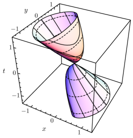
Figure 5: The world-volume of the membrane with $C_{u}=1.1$. The $z$ direction is omitted. The lower world-volume shrinks to a point at $t=x=0$, and the upper expands from there. The dashed lines represent $t=\text{const.}$ slices. The solid lines represent $t+x=\text{const.}$ slices, which also represent the foliating orbits of type ${\text{VII}_{\text{0}}}$–2. The jagged line is a singular orbit of dimension one with $u=0$, which corresponds to the ‘cosmological singularity’ of the intrinsic geometry.

From Eqs. (63), (66) and (67), the metric induced on the world-volume is written as

$$ds_{\Sigma}^{2}=-d\lambda^{2}+u^{2}d\vec{y}\,{}^{2},~{}~{}~{}~{}u(\lambda)\propto\lambda^{1/3},$$ (72)

where we have chosen the parameterization of $\lambda$ so that

$$N(\lambda)=u^{2}(\lambda).$$ (73)

The geometry on the world-volume is analogous to the flat Friedmann-Lemaître-Robertson-Walker universe. At the null line $u=0$ on the world-volume , i.e., $t+x=0$, $y=z=0$, the scalar curvature of the induced metric (72) diverges. Thus, the ‘cosmological singularity’ is described by the null line $u=0$. The orbits (60) and (61) generated by the Killing vectors (52) are two-dimensional spacelike surface, but is null line at $u=0$. Therefore the ‘cosmological singularity’ is described by the singular orbit. We remark that the orbit is singular at $u=0$ but the world-volume (71) itself is smooth everywhere except at the origin of Minkowski spacetime. The embedding of the membrane is very similar to that of the brane universe in five-dimensional anti-de Sitter space Ishihara:2001qe .

VI Summary and discussion

We have investigated the dynamics of cohomogeneity one membranes. The three-dimensional world-volume of the cohomogeneity one membrane is foliated by two-dimensional orbits of the symmetry group $G$ that is a subgroup of the isometry group, $\operatorname{Isom}{\mathcal{M}}$, of the spacetime ${\mathcal{M}}$. The symmetry suggests that the equations of motion are reduced to ordinary differential equations. We have explicitly shown that the Nambu-Goto equations are reduced to the geodesic equations in the orbit space, or the quotient space ${\mathcal{M}}/G$, with a properly defined metric thereon.

In a highly symmetric spacetime, there exist a variety of symmetry groups $G$ that allow two-dimensional orbits. We have proposed a classification of the symmetry groups $G$ under the idea that the orbits of $G$ are equivalent if they are connected by an isometry of ${\mathcal{M}}$. This leads to the classification of the conjugacy classes of $G$ in $\operatorname{Isom}{\mathcal{M}}$. The classification is reduced to that of pairs and triples of Killing vectors which form a Lie algebra. We have presented a concrete procedure of the classification.

We have demonstrated the procedure in Minkowski spacetime and have achieved the complete classification of cohomogeneity one membranes (Tables 3, 4 and 5). The symmetry group $G$ must be of two or three dimensions in order to have a two-dimensional orbits. In Minkowski spacetime, there are two cases for $\dim G=2$: the Abelian group and the non-Abelian group; and four cases for $\dim G=3$: Bianchi type $\text{VI}_{\text{0}}$, $\text{VII}_{\text{0}}$, VIII and IX. The orbits in the latter four cases are two-dimensional maximally symmetric timelike or spacelike surfaces. In addition, because $G$ is a subgroup of $\operatorname{Isom}{\mathcal{M}}$, the embeddings of the orbits should be homogeneous and isotropic. It is interesting that while Bianchi type $\text{VI}_{\text{0}}$, VIII and IX allow, up to geometric equivalence, a unique foliation by the orbits, Bianchi type $\text{VII}_{\text{0}}$ allows two inequivalent foliations by intrinsically flat orbits. One is the flat embedding (Type ${\text{VII}_{\text{0}}}$–1) and the other is an extrinsically curved one (Type ${\text{VII}_{\text{0}}}$–2).

For the membrane of type ${\text{VII}_{\text{0}}}$–2, we have constructed an exact solution. The solution describes a $(2+1)$-dimensional analog of the flat Friedman-Lemaître-Robertson-Walker (FLRW) universe embedded in Minkowski spacetime. The cosmological singularity is represented by a null line on the world-volume. The embedding is similar to that of the flat FLRW brane universe in the five-dimensional anti-de Sitter spacetime Ishihara:2001qe .

Our method is general and can be applied to a higher-dimensional extended object in an arbitrary spacetime. The equations of motion of an extended object becomes a geodesic equations on the orbit space ${\mathcal{M}}/G$. As seen in an example of this article, the solution of the geodesic equations may correspond to a non-trivial configuration of membrane. Therefore the concept of cohomogeneity one objects will be helpful to understand the dynamics of extended objects in spacetime.

*

Appendix A Equivalence classes of ${\cal V}_{\mathrm{C}}^{\mathrm{I}}$

We give simple representatives of equivalence classes in ${\cal V}_{\mathrm{C}}^{\mathrm{I}}$, which consists of pairs of commuting Killing vectors $(\boldsymbol{\xi}_{1},\,\boldsymbol{\xi}_{2})$, where $\boldsymbol{\xi}_{1}$ is in the canonical form of Type I, i.e.,

$$\boldsymbol{\xi}_{1}=a\boldsymbol{P}\kern-1.0pt_{t}+b\boldsymbol{L}_{z},\ \ \ (a,b:\text{arbitrary constant}).$$ (74)

In the case of $a\neq 0$ and $b\neq 0$, the general form of $\boldsymbol{\xi}_{2}$ which commutes with $\boldsymbol{\xi}_{1}$ is simply

$$\boldsymbol{\xi}_{2}=a^{\prime}\boldsymbol{P}\kern-1.0pt_{t}+b^{\prime}\boldsymbol{L}_{z}+c^{\prime}\boldsymbol{P}\kern-1.0pt_{z},$$ (75)

where $a^{\prime}$, $b^{\prime}$ and $c^{\prime}$ are constants. We require

$$ab^{\prime}-ba^{\prime}\neq 0$$ (76)

or

$$c^{\prime}\neq 0$$ (77)

so that $\boldsymbol{\xi}_{1}$ and $\boldsymbol{\xi}_{2}$ are linearly independent.

By virtue of the equivalence under $\text{GL}(2,R)$ action, we can reduce the form of $(\boldsymbol{\xi}_{1},\,\boldsymbol{\xi}_{2})$ to a simple one. For $\boldsymbol{\xi}_{2}$ satisfying Eq. (76), we have

$$(\boldsymbol{\xi}_{1},\,\boldsymbol{\xi}_{2})=(\boldsymbol{P}\kern-1.0pt_{t}+c\boldsymbol{P}\kern-1.0pt_{z},\,a^{\prime}\boldsymbol{P}\kern-1.0pt_{t}+b^{\prime}\boldsymbol{L}_{z}+c^{\prime}\boldsymbol{P}\kern-1.0pt_{z})$$ (78)

where $c$ is a constant determined by $a$, $b$, $a^{\prime}$, $b^{\prime}$ and $c^{\prime}$. Otherwise, for $\boldsymbol{\xi}_{2}=\boldsymbol{P}\kern-1.0pt_{z}$, we have

$$(\boldsymbol{\xi}_{1},\,\boldsymbol{\xi}_{2})=(a\boldsymbol{P}\kern-1.0pt_{t}+b\boldsymbol{L}_{z},\,\boldsymbol{P}\kern-1.0pt_{z}).$$ (79)

For further reduction of the pair (78), we take an isometry $\phi$ generated by $\boldsymbol{K}\kern-1.0pt_{z}$, namely Lorentz boost for $z$ direction . The Killing vector $\boldsymbol{\xi}_{1}=\boldsymbol{P}\kern-1.0pt_{t}+c\boldsymbol{P}\kern-1.0pt_{z}$ is transformed to

$${\phi}_{\ast}\boldsymbol{\xi}_{1}=(\cosh\theta+c\sinh\theta)\boldsymbol{P}\kern-1.0pt_{t}+(c\cosh\theta+\sinh\theta)\boldsymbol{P}\kern-1.0pt_{z}.$$ (80)

Choosing the parameter $\theta$ so that

$$c\cosh\theta+\sinh\theta =0\ \ \text{for $|c|<1$},$$ (81)

$$\cosh\theta+c\sinh\theta =0\ \ \text{for $|c|>1$},$$ (82)

we can reduce the form of the pair (78) to

$$(\boldsymbol{\xi}_{1},\,\boldsymbol{\xi}_{2})=\begin{cases}(\boldsymbol{P}\kern-1.0pt_{t},\,a^{\prime\prime}\boldsymbol{P}\kern-1.0pt_{t}+b^{\prime}\boldsymbol{L}_{z}+c^{\prime\prime}\boldsymbol{P}\kern-1.0pt_{z})\ \ \text{for $|c|<1$, }\\ (\boldsymbol{P}\kern-1.0pt_{z},\,a^{\prime\prime}\boldsymbol{P}\kern-1.0pt_{t}+b^{\prime}\boldsymbol{L}_{z}+c^{\prime\prime}\boldsymbol{P}\kern-1.0pt_{z})\ \ \text{for $|c|>1$. }\\ \end{cases}$$ (83)

In the case $|c|=1$, $\boldsymbol{\xi}_{1}(=\boldsymbol{P}\kern-1.0pt_{t}\pm\boldsymbol{P}\kern-1.0pt_{z})$ is invariant under the Lorentz boost $\phi$. Using $\text{GL}(2,R)$ action again, we have three kinds of representatives,

$$(\boldsymbol{\xi}_{1},\,\boldsymbol{\xi}_{2})=\begin{cases}(\boldsymbol{P}\kern-1.0pt_{t},\,c^{\prime\prime}\boldsymbol{P}\kern-1.0pt_{z}+b^{\prime}\boldsymbol{L}_{z}),\\ (\boldsymbol{P}\kern-1.0pt_{z},\,a^{\prime\prime}\boldsymbol{P}\kern-1.0pt_{t}+b^{\prime}\boldsymbol{L}_{z}),\\ (\boldsymbol{P}\kern-1.0pt_{t}+\boldsymbol{P}\kern-1.0pt_{z},\,a^{\prime\prime}\boldsymbol{P}\kern-1.0pt_{t}+b^{\prime}\boldsymbol{L}_{z}).\end{cases}$$ (84)

We should note that the pair (79) is included in the second case of (84). Therefore these three kinds are the conclusive representatives of ${\cal V}_{\mathrm{C}}^{\mathrm{I}}$ within the case $a,b\neq 0$. It should also be noted that pairs with different values of constants $a^{\prime\prime}$, $b^{\prime}$ and $c^{\prime\prime}$ except for overall scaling of $\boldsymbol{\xi}_{2}$ are not equivalent.

References

- (1) L. Randall and R. Sundrum, Phys. Rev. Lett. 83, 3370 (1999)
- (2) J. M. Maldacena, Adv. Theor. Math. Phys. 2, 231 (1998)
- (3) V. P. Frolov, V. Skarzhinsky, A. Zelnikov and O. Heinrich, Phys. Lett. B 224, 255 (1989)
- (4) H. J. de Vega, A. L. Larsen and N. G. Sanchez, Nucl. Phys. B 427, 643 (1994)
- (5) A. L. Larsen and N. G. Sanchez, Phys. Rev. D 50, 7493 (1994)
- (6) Larsen A L and Sanchez N G, Phys. Rev. D 51 6929 (1995)
- (7) de Vega H J and Egusquiza I L, Phys. Rev. D 54 7513 (1996)
- (8) V. P. Frolov, S. Hendy and J. P. De Villiers, Class. Quant. Grav. 14, 1099 (1997)
- (9) Ogawa K, Ishihara H, Kozaki H, Nakano H and Saito S, Phys. Rev. D 78 023525 (2008)
- (10) Ishihara H and Kozaki H, Phys. Rev. D 72 061701(R) (2005)
- (11) Koike T, Kozaki H and Ishihara H, Phys. Rev. D 77 125003 (2008)
- (12) H. Kozaki, T. Koike and H. Ishihara, Class. Quant. Grav. 27, 105006 (2010)
- (13) T. Igata and H. Ishihara, Phys. Rev. D 81, 044024 (2010).
- (14) T. Igata and H. Ishihara, Phys. Rev. D 82, 044014 (2010).
- (15) D. Kubiznak and V. P. Frolov, JHEP 0802, 007 (2008)
- (16) H. Goenner and J. Stachel, J. Math. Phys. 11, 3358 (1970)
- (17) H. Stephani, D. Kramer, M. A. H. MacCallum and C. Hoenselaers, Exact Solutions of Einstein’s Field Equations (Cambridge University Press, Cambridge, 2003)
- (18) H. Ishihara, Phys. Rev. D 66, 023513 (2002)