October 21th, 2014

REFRACTIVE PROPERTIES OF GRAPHENE IN A MEDIUM-STRONG EXTERNAL MAGNETIC FIELD

O. Coquand ,  B. Machet

Abstract: 1-loop quantum corrections are shown to induce large effects on the refractive index $n$ inside a graphene strip in the presence of a constant and uniform external magnetic field $B$ orthogonal to it. To this purpose, we use the tools of Quantum Field Theory to calculate the photon propagator at 1-loop inside graphene in position space, which leads to an effective vacuum polarization in a brane-like theory of photons interacting with massless electrons at locations confined inside the thin strip (its longitudinal spread is considered to be infinite). The effects factorize into quantum ones, controlled by the value of $B$ and that of the electromagnetic coupling $\alpha$, and a transmittance function $U$ in which the geometry of the sample and the resulting confinement of the $\gamma\,e^{+}e^{-}$ vertices play major roles. They only concern the so-called “transverse-magnetic” polarization of photons, which suggests (anisotropic) electronic spin resonance of the graphene-born virtual electrons. We consider photons inside the visible spectrum and magnetic fields in the range 1-20  Tesla. At $B=0$, quantum effects depend very weakly on $\alpha$ and $n$ is essentially controlled by $U$; we recover, then, an opacity for visible light of the same order of magnitude $\pi\alpha_{vac}$ as measured experimentally.

1 Introduction. Main features of the calculation

Constant magnetic fields $B$ can induce, through the screening of the Coulomb potential, dramatic effects on the spectrum of hydrogen and on the critical number $Z_{c}$ of atoms [1][2] [3]. However, typical effects being ${\cal O}(\frac{\alpha\hbar eB}{m_{e}^{2}c^{2}})$, gigantic fields are needed, $B\geq 10^{12}\,T$, which are out of reach on earth. It was also shown in [4] that such extreme “supercritical” magnetic fields could strongly modify the refraction of light. The property that the fine structure constant $\alpha$ in graphene largely exceeds $1$ [5] instead of its vacuum value $\alpha_{vac}\simeq\frac{1}{137}$ was a sufficient motivation to investigate whether sizable effects could be obtained at lower cost in there.

While graphene in a constant, uniform external magnetic field is usually associated with the so-called “abnormal quantum hall effect” [5] [6], we have found that one can also expect optical effects for electromagnetic waves in the visible spectrum and at “reasonable” values of the external $B$ not exceeding $20\,T$.

Since we are concerned with the refractive index, the main object of our study is the propagator of the photon (with incoming momentum $q$) inside graphene, and, more specially its quantum corrections at 1-loop. They originate from the creation, inside the medium, of virtual $e^{+}e^{-}$ pairs, which can then propagate everywhere before annihilating, again inside graphene. We therefore need to constrain the two $\gamma\,e^{+}e^{-}$ vertices to lie in the interval $[-a,+a]$ along the direction $z$ of the magnetic field, perpendicular to the surface of graphene. To this purpose, we evaluate the photon propagator in position space, and integrate the “$z$” coordinates of the two vertices from $-a$ to $+a$ instead of the usual infinite interval of customary Quantum Field Theory. This strategy sets of course the intrinsic limitation of our calculations that they are only valid inside graphene.

The next feature to be accounted for is that, in the close vicinity of the Dirac points of graphene, electronic excitations are massless with a linear dispersion relation of the type $p_{0}=v_{F}|\vec{p}|$, where $p_{0}$ is the energy of the particle and $v_{F}$ is the Fermi velocity $v_{F}\ll c$ [5] [6]. This is obtained in the tight-binding approximation, which leads to a massless Dirac-like Hamiltonian for these excitations, in which $c$ is replaced with $v_{F}$. This raises the issue of which electronic propagator we have to insert in the quantum loop. At first sight, the natural candidate corresponds to the massless Lagrangian

$$\bar{\psi}\left(\gamma_{0}p_{0}-v_{F}(\gamma_{1}p_{1}-\gamma_{2}p_{2}-\bcancel{\gamma_{3}p_{3}})-\bcancel{mc}^{2}\right)\psi$$ (1)

(we have restored the appropriate factors with dimension $[velocity]$), which corresponds to the effective Dirac-like Hamiltonian of graphene electrons. However, as explained in subsection 4.1.1, there are strong motivations for putting inside the loop Dirac-like excitations propagating like in vacuum, that is with $c$ instead of $v_{F}$. The first is that, while electron/positron excitations are created and annihilated inside graphene, they can then propagate in the whole space. Actually, for the idealized graphene strip with infinite horizontal spreading $L\to\infty$ that we are considering, the Coulomb energy of an electron, expected to vary like $1/L$, can be neglected, and virtual electrons spend much more time in the “bulk” (outer space) than inside graphene. The second reason concerns energy-momentum conservation at the vertices .
The last issues concern whether we may keep $m=0$ and $p_{3}=0$. When doing a perturbative expansion, propagators of internal lines are always the ones corresponding to the classical Lagrangian. In the problem under scrutiny, internal electron lines must therefore correspond to the effective classical Hamiltonian of graphene at the Dirac points. Since doing perturbation amounts to calculating quantum fluctuations, this choice amounts to selecting a “classical” starting point (vacuum) for perturbation theory, which is “graphene”. Would quantum corrections trigger, for example, large “chiral symmetry breaking”, serious doubts should be cast on this choice and on the reliability of the procedure (there are good reasons to think that we are safe, look for example at subsection 5.9).
Therefore, the propagator of virtual electrons that we shall use is that of massless Dirac electrons with $p_{3}=0$ which propagate like in vacuum, but in the presence of a constant, uniform external $B$; its expression is given by the Schwinger formalism [7] [8]. That no $v_{F}$ is introduced in there makes finally that the Fermi velocity appears nowhere in our formulæ, except, implicitly, inside the electromagnetic coupling $\alpha$ that we shall vary from its vacuum value $\alpha_{vac}=\frac{e^{2}}{4\pi\epsilon_{0}\hbar c}=\frac{1}{137}$ up to $\alpha\simeq 2$, which roughly corresponds to its effective value inside graphene .

The calculation of the photon propagator at 1-loop yields a 1-loop vacuum polarization tensor $\Pi^{\mu\nu}$ that can be plugged in the light-cone equations derived according to the pioneering work of Tsai and Erber [9], and of Dittrich and Gies [10]. One of the salient features of $\Pi^{\mu\nu}$ is that it factorizes into a tensor $T^{\mu\nu}(\hat{q},B)$, which depends on $B$, $\hat{q}\equiv(q_{0},q_{1},q_{2})$ and on the electromagnetic coupling $\alpha$, $\times$ a universal function $U$ which does not depend on the magnetic field, nor of $\alpha$. While $U$ carries information concerning the geometry of the sample and the confinement of the vertices, and shares similarities with the so called “transmittance” function in optics or “transfer function” in electronics, $T^{\mu\nu}(\hat{q},B)$ gathers quantum effects and those of the magnetic field. Its components $\mu,\nu=0,1,2$ are reminiscent of those of vacuum polarization in $2+1$ dimensions in the presence of $B$; however, for the system under concern, $T^{33}=-T^{00}\not=0$ plays the dominant role. At the limit $B=\infty$ they are the only components that subsist, as expected from the $D\to D-2$ dimensional reduction that takes place in this case (see for example[11]) (only the $0$ and $3$ components of the photon then couple).

From the dimensional point of view, we consider the graphene strip as a truly 3+1 dimensional object, the thickness $2a$ of which is very small as compared with its flat extension; nowhere have we made the premise that the underlying physics is 2+1 dimensional. Classically, virtual electron-positron pairs created at the lowest Landau level on the Dirac cone have a vanishing momentum $p_{3}=0$ in the direction of $B$; however, the large quantum fluctuations $\sim\hbar/a$ that arise due to the confinement of $\gamma\,e^{+}e^{-}$ vertices inside the medium allow them to eventually evolve in the whole 3+1 space. In this setup, the direction of $B$ has a twofold importance: first, due to the dimensional reduction $D\to D-2$ mentioned above; secondly because the vertex confinement and the related quantum fluctuations and momentum exchanges largely influence the behavior of the refractive index. In particular, forgetting about $a\not=0$ erases the transmittance function and the leading $1/\sin\theta$ behavior of the refractive index.

The quantum fluctuations of electronic momentum in the direction of $B$ get transferred to the photon. That the resulting photonic momentum non-conservation should not exceed $\hbar/a$ yields a quantum upper bound $n\leq n_{quant}$ for the refractive index.

The effects of confinement that we exhibit should not be put hastily in correspondence with the ones that have, for example, been investigated in [12] for a finite longitudinal size $L$ of graphene. A major difference is indeed that we are concerned here with the confinement in the “short” direction, the thickness $2a\approx 350\,pm$, considering that its longitudinal spread $L$ is infinite . This makes the physical interpretation less intuitive since no cyclotron radius can eventually, in our case, match the size of graphene. However, our results exhibit the remarkable property that, again in relation with the dimensional reduction that takes place in the presence of a strong external $B$, only the propagation of photons with “parallel” polarization gets concerned (for the transverse polarization, the only solution that we found to the light-cone equation is the trivial $n=1$). In this state of polarization, the oscillating magnetic field of the electromagnetic wave is orthogonal to the external constant $B$, which is a typical situation to induce the magnetic resonance of the spins of the graphene-born electrons. Electron spin resonance may thus be at the origin of the large sensitivity of the refractive index to the external $B$. The large value of the electromagnetic coupling also participates to producing macroscopic effects.

The refractive index $n=n_{1}+i\,n_{2}$ is found to essentially depend on $\alpha$, on the angle of incidence $\theta$, and on the ratio $\Upsilon=\frac{c\sqrt{2\hbar eB}}{q_{0}}$. In the absence of any external $B$, its dependence on the electromagnetic coupling fades away, and it is mainly constrained by the sole property that electrons are created and annihilated inside graphene.

A transition occurs at small angle of incidence $\theta_{min}\sim\frac{1}{\Upsilon}$: no non-trivial solution with $|n_{2}|\ll n_{1}$ to the light-cone equation exists anymore for $\theta<\theta_{min}$. This also corresponds to $|n|\leq n_{max}\sim\Upsilon$. Since at $\theta=0$ (normal incidence), the only solution to the light-cone equation is the trivial $n=1$, getting reliable results in the zone of transition from $\theta_{min}$ down to $\theta=0$ requires more elaborate numerical techniques, which is left for a subsequent work.

Our calculations and the corresponding expansions are made in the limit of a “medium-strong” $B$, in the sense that $\sqrt{2\hbar eB}\gg q_{0}/c$, and are only valid at this limit such that, in particular, the limit $B\to 0$ cannot be taken. $B$ is however not considered to be “infinite” like in [2] [3] [13]. In practice, in the case at hand, the leading terms in the expansion of the electronic propagators in powers of $1/\tau eB\ll 1$ ($\tau$ is the proper time) do not contribute to the refractive index. The effects originate from the subleading terms, and the final growing like $\sqrt{eB}$ of the relevant components of the vacuum polarization tensor comes from the integration over the transverse electronic degrees of freedom.

Expansions are also done at small values of the parameter $\eta=\frac{aq_{0}}{\hbar c}$. This condition is always satisfied for optical frequencies. It also guarantees to stay in the linear part of the electron spectrum close to the Dirac point, which is an essential ingredient to use a “Dirac-like” effective Hamiltonian [5].

We are concerned with photons in the visible spectrum, which sets us very far from geometrical optics, since the corresponding wavelengths are roughly three orders of magnitude larger that the thickness $2a$ of graphene.

We limit $B$, for the sake of experimental feasibility, to $20\,T$. This upper bound also guarantees that the 4-fold degeneracy of the Landau level at the Dirac point does not yet get lifted [14].

Our results are summarized on the two plots of Figure 5.

The last section deals with the case $B=0$, for which a dedicated calculation is needed. We show in this case that no $\theta_{min}$ exists and that, instead, as the angle of incidence gets smaller and smaller, the refractive index $n$ goes continuously from “quasi-real” values to complex values with larger $n_{1}$ and $n_{2}$. At very small values of $\theta$, we recover an opacity of the same order of magnitude as the one measured experimentally [15]. However, the same problem as for $B\not=0$ exists concerning a smooth transition to $\theta=0$. In addition, for $\alpha>1$, the index diverges at $s_{\theta}^{2}\geq\frac{1}{\alpha}$, expressing problems of a fixed-order perturbative expansion at strong coupling.

The paper is intended to be self-contained. The amount of literature dedicated to graphene is very large and we cannot, unfortunately, pay a fair tribute to the whole of it. We only cite the works that have been the most used for writing the present one, but the reader can find, in particular inside the review articles, references to most of the important papers.

2 From the vacuum polarization to light-cone equations and to the refractive index

2.1 Conventions and settings. Notations

Following Tsai-Erber [9], the constant and uniform magnetic field $\vec{B}$ is chosen to be parallel to the $z$ axis and the wave vector $\vec{q}$ of the propagating photon to lie in the $(x,z)$ plane (see Figure 1) .

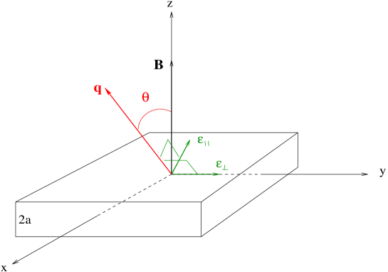
Figure 1: $\vec{B}$ is perpendicular to the graphene strip of width $2a$. The polarization vector $\vec{\epsilon}$, perpendicular to the momentum $\vec{q}$ of the electromagnetic wave, is decomposed into $\vec{\epsilon}_{\parallel}$ in the $(x,z)$ plane and $\vec{\epsilon}_{\perp}$ perpendicular to this plane.

The $(\vec{B},\vec{q})$ angle $\theta$ is the “angle of incidence”; since we are concerned with the propagation of light inside graphene, $\theta$ is the angle of incidence of light inside this medium. The plane $(x,z)$ is the plane of incidence.

The polarization vector $\vec{\epsilon}$  (which, by convention, refers to the electric field) is decomposed into $\vec{\epsilon}_{\parallel}=-\cos\theta\,\vec{i}+\sin\theta\,\vec{k}$, in the $(x,z)$ plane, and $\vec{\epsilon}_{\perp}\parallel\vec{j}$, both orthogonal to $\vec{q}$ ($\vec{i},\vec{j},\vec{k}$ are the unit vectors along the $x,y,z$ axes). One has $\vec{q}=|\vec{q}|\,(\sin\theta\,\vec{i}+\cos\theta\,\vec{k})$. $\vec{\epsilon}_{\parallel}$ is called “parallel polarization” and $\vec{\epsilon}_{\perp}$ “transverse polarization”. They are also called respectively “transverse magnetic” and “transverse electric” by reference to plane waves. It must be noticed that, at normal incidence $\theta=0$, there is no longer a plane $(\vec{q},\vec{B})$ such that these two polarizations can no longer be distinguished.

We shall in the following use “hatted” letters for vectors living in the Lorentz subspace $(0,1,2)$. For example

$$\hat{q}=(q^{0},q^{1},q^{2}),\quad q=(\hat{q},q_{3})=(q_{0},q_{1},q_{2},q_{3})=(q_{0},\vec{q}).$$ (2)

Throughout this work we use the metric $(+,-,-,-)$ and mostly work in the International Unit System (SI). It is however often convenient to express energies in $eV$.

2.2 The modified Maxwell Lagrangian and the light-cone equations

Figure 2: The vacuum polarization $\Pi^{\mu\nu}(q)$.

Taking into account the contribution of the vacuum polarization $\Pi_{\mu\nu}$ (see Figure 2) that we shall calculate in section 3, the Maxwell Lagrangian $-\frac{1}{4}F_{\mu\nu}(x)F^{\mu\nu}(x)$ gets modified to [10]

$${\cal L}(x,B)=-\frac{1}{4}F_{\mu\nu}(x)F^{\mu\nu}(x)-\frac{1}{2}\int d^{4}y\;A^{\mu}(x)\Pi_{\mu\nu}(x,y,B)A^{\nu}(y),$$ (3)

from which one gets the Euler-Lagrange equation

$$\Big{(}g_{\mu\nu}\,q^{2}-q_{\mu}q_{\nu}+\Pi_{\mu\nu}(q,B)\Big{)}A^{\nu}(q)=0.$$ (4)

Left-multiplying (4) with

$$A^{\mu}=\beta_{1}\,\epsilon^{\mu}_{\perp}+\beta_{2}\,\epsilon^{\mu}_{\parallel},$$ (5)

yields the light-cone equation

$$\begin{split}&(\beta_{1}\epsilon^{\mu}_{\perp}+\beta_{2}\epsilon^{\mu}_{\parallel})\Big{(}g_{\mu\nu}\,q^{2}-q_{\mu}q_{\nu}+\Pi_{\mu\nu}(q,B)\Big{)}(\beta_{1}\epsilon^{\nu}_{\perp}+\beta_{2}\epsilon^{\nu}_{\parallel})=0,\cr&\epsilon^{\mu}_{\perp}=(0,0,1,0),\quad\epsilon^{\mu}_{\parallel}=(0,-c_{\theta},0,s_{\theta}),\qquad c_{\theta}\equiv\cos\theta,\ s_{\theta}\equiv\sin\theta.\end{split}$$ (6)

As we shall see in sections 3 and 4, $\Pi^{03}=0=\Pi^{13}=\Pi^{23}$, such the light-cone equation (6) simplifies to

$$(\beta_{1}^{2}+\beta_{2}^{2})q^{2}+\left(\beta_{1}^{2}\Pi^{22}(q,B)+\beta_{2}^{2}\left(c_{\theta}^{2}\;\Pi^{11}(q,B)+s_{\theta}^{2}\;\Pi^{33}(q,B)\right)+2\beta_{1}\beta_{2}\,c_{\theta}\,\Pi^{12}(q,B)\right)=0.$$ (7)

$\vec{q}$ has been furthermore chosen to lie in the $(x,z)$ plane, so $q_{2}=0$, which entails (see (58)) $\Pi^{02}=0=\Pi^{20},\Pi^{12}=0=\Pi^{21}$, and the light-cone equation finally shrinks to

$$(\beta_{1}^{2}+\beta_{2}^{2})\,q^{2}+\left(\beta_{1}^{2}\,\Pi^{22}(q,B)+\beta_{2}^{2}\left(c_{\theta}^{2}\;\Pi^{11}(q,B)+s_{\theta}^{2}\;\Pi^{33}(q,B)\right)\right)=0.$$ (8)

Depending of the polarization of the photon, there are accordingly two different light-cone relations:
$\bullet$ for $A^{\mu}_{\perp}(q_{0},q_{1},0,q_{3})$, $\beta_{1}=1,\beta_{2}=0$,

$$q^{2}+\Pi^{22}(q,B)=0;$$ (9)

$\bullet$  for $A^{\mu}_{\parallel}(q_{0},q_{1},0,q_{3})$, $\beta_{1}=0,\beta_{2}=1$,

$$q^{2}+\Big{(}c_{\theta}^{2}\;\Pi^{11}(q,B)+s_{\theta}^{2}\;\Pi^{33}(q,B)\Big{)}=0.$$ (10)

Notice the occurrence of $\Pi^{33}$ in (10), which plays a major role and would not be there in $QED_{2+1}$ .

A remark is due concerning eq. (4). Its derivation from the effective Lagrangian (3) relies on the property that, in position space, $\Pi^{\mu\nu}(x,y)$ is in reality a function of $(x-y)$ only. This is however, as we shall see, not exactly the case here. $\Pi^{\mu\nu}$ depends indeed on $(\hat{x}-\hat{y})$ but individually on $x_{3}$ and $y_{3}$ (see the first remark at the end of subsection 3.1.2). Once the dependence on $(x_{3}-y_{3})$ has been extracted, there is a left-over dependence on $y_{3}$, which finally yields for our results the dependence of the refractive index on $u=\frac{y_{3}}{a}\in[-1,+1]$. We shall see however that this dependence is always extremely weak, and we consider therefore the Euler-Lagrange equation (4) to be valid to a very good approximation.

2.3 The refractive index $\boldsymbol{n}$

We define it in a standard way by

$$n=\frac{c|\vec{q}|}{q_{0}}.$$ (11)

In practice, $\Pi^{\mu\nu}$ is not only a function of $q$ and $B$, but of the angle of incidence $\theta$ and of the relative depth $u$ inside the graphene strip, $u\in[-1,+1]$. The light-cone equations therefore translate into relations $n=n(\theta,B,q_{0},u)$ that we will write explicitly in section 5, after calculating the vacuum polarization.

3 The photon propagator in $\boldsymbol{x}$-space and the vacuum polarization $\boldsymbol{\Pi^{\mu\nu}}$

The vacuum polarization $\Pi^{\mu\nu}$ to be introduced inside the light-cone equations (9,10) is obtained by calculating the photon propagator in position-space, while confining, at the two vertices $\gamma\,e^{+}e^{-}$, the corresponding $z$’s to lie inside graphene, $z\in[-a,a]$.

It factorizes into $\Pi^{\mu\nu}(\hat{q},q_{3},\frac{y_{3}}{a},B)=\frac{1}{\pi^{2}}\;T^{\mu\nu}(\hat{q},B)\;U(\hat{q},q_{3},\frac{y_{3}}{a})$ in which $U$ is a universal function that does not depend on the magnetic field, nor on $\alpha$, that we also encounter when dealing with the case of no external $B$. It is the Fourier transform of the product of two functions: the first, $\frac{\sin ak_{3}}{ak_{3}}$, is the Fourier transform of the “gate function” corresponding to the graphene strip along $z$; the second carries the remaining information attached to the confinement of the vertices. Its analytical properties inside the complex plane control in particular the “leading” $\frac{1}{\sin\theta}$ behavior of the refractive index inside graphene. The integration variable of this Fourier transform is $k_{3}$, the difference between the momenta along $B$ of the outgoing and incoming photons (see below).

This factorization can be traced back to $T^{\mu\nu}$ not depending on $q_{3}$, for the simple reason that the propagators of electrons inside graphene are evaluated at vanishing “$p_{3}$” momentum (in the direction of the external $B$). An example of how factors combine is the following. $\Pi^{\mu\nu}$ still includes an integration on $p_{3}$, which factors out. That the interactions of electrons are confined along $B$ triggers quantum fluctuations of their momentum in this direction. Setting an ultraviolet cutoff $\pm\frac{\hbar}{a}$ on the $p_{3}$ integration (saturating the Heisenberg uncertainty relation) makes this integral proportional to $\frac{1}{a}$. This factor completes, inside the integral $\int dk_{3}$ defining $U$, the “geometric” $\frac{\sin ak_{3}}{ak_{3}}$ evoked above.

$k_{3}=s_{3}-q_{3}$ represents the amount of momentum non-conservation of photons in the direction of $B$: it occurs by momentum exchange between photons and (the quantum momentum fluctuations of) electrons. The integration $dk_{3}$ gets bounded by the rapid decrease of $\frac{\sin ak_{3}}{ak_{3}}$ for $|k_{3}|$ larger than $\frac{\hbar}{a}$ and this upper bound $|k_{3}|\leq\frac{\hbar}{a}$ is the same as the one that we set for quantum fluctuations of the electron momentum $p_{3}$. So, the energy-momentum non-conservation between the outgoing and incoming photons cannot exceed the uncertainty on the momentum of electrons due to the confinement of vertices. Momentum conservation for the photon is only recovered when $a\to\infty$ (limit of “standard” QFT).

3.1 The 1-loop photon propagator in position space

We calculate the 1-loop photon propagator

$$\Delta^{\rho\sigma}(x,y)=\langle 0|TA^{\rho}(x)A^{\sigma}(y)|0\rangle$$ (12)

and somewhat lighten the notations, omitting symbols like T-product, …, writing for example $G(\hat{p})$ for $G(\hat{p},B)$ etc.

Introducing the coordinates $u=(u_{0},u_{1},u_{2},u_{3})$ and $v=(v_{0},v_{1},v_{2},v_{3})$ of the two $\gamma\,e^{+}e^{-}$ vertices one gets at 1-loop

$$\Delta^{\rho\sigma}(x,y)=\int d^{4}u\int d^{4}v\;A^{\rho}(x)[(ie)A^{\mu}(u)\bar{\psi}(u)\gamma_{\mu}\psi(u)][(ie)A^{\nu}(v)\bar{\psi}(v)\gamma_{\nu}\psi(v)]A^{\sigma}(y).$$ (13)

Making the contractions for fermions etc …yields

$$\begin{split}\Delta^{\rho\sigma}(x,y)&=e^{2}\int d^{4}u\int d^{4}v\;Tr\int\frac{d^{4}q}{(2\pi)^{4}}\;e^{iq(u-x)}\Delta^{\rho\mu}(q)\gamma_{\mu}\int\frac{d^{4}p}{(2\pi)^{4}}\;e^{ip(u-v)}G(p)\gamma_{\nu}\cr&\hskip 113.81102pt\int\frac{d^{4}r}{(2\pi)^{4}}\;e^{ir(v-u)}G(r)\int\frac{d^{4}s}{(2\pi)^{4}}\;e^{is(y-v)}\Delta^{\sigma\nu}(s).\end{split}$$ (14)

In what follows we shall also omit the trace symbol “$Tr$”.

3.1.1 “Standard” Quantum Field Theory

One integrates $\int_{-\infty}^{+\infty}d^{4}u$ and $\int_{-\infty}^{+\infty}d^{4}v$ for the four components of $u$ and $v$. This gives:

$$\Delta^{\rho\sigma}(x,y)=\int\frac{d^{4}q}{(2\pi)^{4}}\;e^{-iq(x-y)}\Delta^{\rho\mu}(q)\Delta^{\nu\sigma}(q)\underbrace{e^{2}\int\frac{d^{4}p}{(2\pi)^{4}}\;\gamma_{\mu}G(p)\gamma_{\nu}G(p+q)}_{i\Pi_{\mu\nu}(q)}.$$ (15)

To obtain the sought for vacuum polarization, the two external photon propagators $\Delta^{\rho\mu}(q)$ and $\Delta^{\nu\sigma}(q)$ have to be truncated, which gives the customary expression

$$i\Pi_{\mu\nu}(q)=+e^{2}\int\frac{d^{4}p}{(2\pi)^{4}}\;\gamma_{\mu}G(p)\gamma_{\nu}G(p+q).$$ (16)

3.1.2 The case of graphene. $\boldsymbol{\gamma\,e^{+}e^{-}}$ vertices confined along $\boldsymbol{z}$ : $\boldsymbol{\Pi^{\mu\nu}=\frac{1}{\pi^{2}}\;T^{\mu\nu}\times U}$

The coordinates $u_{3}$ and $v_{3}$ of the two vertices we do not integrate anymore $\int_{-\infty}^{+\infty}$ but only $\int_{-a}^{+a}$ in which $2a$ is the thickness of the graphene strip. This restriction localizes the interactions of electrons with photons inside graphene.

So doing, the results that we get are only valid inside graphene, and we therefore only focus on the “optical properties” of graphene. Photons also interact with electrons outside graphene but this is not of concern to us since we are studying how the propagation of photons is influenced by their interactions with electrons inside the medium.

Decomposing in (14) $du=d^{3}\hat{u}\,du_{3},\;dv=d^{3}\hat{v}\,dv_{3}$, we get by standard manipulations (see Appendix A)

$$\begin{split}\Delta^{\rho\sigma}(x,y)&=\int\frac{dp_{3}}{2\pi}\int\frac{dq_{3}}{2\pi}\int\frac{dr_{3}}{2\pi}\int\frac{ds_{3}}{2\pi}\int_{-a}^{+a}du_{3}\;e^{iu_{3}(q_{3}+p_{3}-r_{3})}\int_{-a}^{+a}dv_{3}\;e^{iv_{3}(-p_{3}+r_{3}-s_{3})}\cr&\int\frac{d^{3}\hat{q}}{(2\pi)^{3}}\;e^{i\hat{q}(\hat{y}-\hat{x})}e^{iq_{3}(-x_{3})}e^{is_{3}(y_{3})}\Delta^{\rho\mu}(\hat{q},q_{3})\Delta^{\sigma\nu}(\hat{q},s_{3})\ \underbrace{e^{2}\int\frac{d^{3}\hat{p}}{(2\pi)^{3}}\;\gamma_{\mu}G(\hat{p},B)\gamma_{\nu}G(\hat{p}+\hat{q},B)}_{iT_{\mu\nu}(\hat{q},B)},\end{split}$$ (17)

in which we introduced the tensor $T_{\mu\nu}(\hat{q},B)$ that is calculated in section 4.

One of the main difference with standard QFT (subsection 3.1.1) is that the tensor $T_{\mu\nu}$ that arises instead of the $\Pi_{\mu\nu}$ (16) does not depend on $q_{3}$, but only on $\hat{q}$. The reason is that, as already mentioned, the propagators of electrons in the loop are evaluated at vanishing momentum in the direction of $B$. The calculation of $T_{\mu\nu}$ is performed in section 4. There, the explicit form of the electron propagator in external $B$ will also be given. Let us just notice here that, by its definition (see (17) and (35)), the components $\mu,\nu=0,1,2$ of $T_{\mu\nu}$ are those of a 2+1 dimensional vacuum polarization (in which the integration runs over the variables $(p_{0},p_{1},p_{2})$). However, the Lorentz indices $\mu,\nu$ extend to 3 and, furthermore, it is precisely $T_{33}$ that will play the leading role to determine the refractive index. The corresponding physics cannot manifestly be reduced to 2+1 dimensions.

Notice that, despite the “classical” input $p_{3}=0$ for electrons created inside graphene on the Dirac cone (see subsection 4.1), the photon propagator still involves the integration $\int dp_{3}$.

Now,

$$\int_{-a}^{+a}dx\;e^{itx}=2\frac{\sin at}{t},$$ (18)

such that

$$\begin{split}&\Delta^{\rho\sigma}(x,y)=4\int\frac{dq_{3}}{2\pi}\int\frac{ds_{3}}{2\pi}e^{i(s_{3}y_{3}-q_{3}x_{3})}L(a,s_{3},q_{3})\int\frac{d^{3}\hat{q}}{(2\pi)^{3}}\;e^{i\hat{q}(\hat{y}-\hat{x})}\Delta^{\rho\mu}(\hat{q},q_{3})\Delta^{\sigma\nu}(\hat{q},s_{3})\;iT_{\mu\nu}(\hat{q},B),\cr&\hskip 85.35826pt\text{with}\quad L(a,s_{3},q_{3})=\int_{-\infty}^{+\infty}\frac{dp_{3}}{2\pi}\frac{dr_{3}}{2\pi}\;\frac{\sin a(q_{3}+p_{3}-r_{3})}{q_{3}+p_{3}-r_{3}}\;\frac{\sin a(r_{3}-p_{3}-s_{3})}{r_{3}-p_{3}-s_{3}}.\end{split}$$ (19)

Going from the variables $r_{3},p_{3}$ to the variables $p_{3},h_{3}=r_{3}-p_{3}$ leads to

$$L(a,s_{3},q_{3})=\int_{-\infty}^{+\infty}\frac{dp_{3}}{2\pi}\;K(a,s_{3},q_{3}),\quad\text{with}\quad K(a,s_{3},q_{3})=\int_{-\infty}^{+\infty}\frac{dh_{3}}{2\pi}\;\frac{\sin a(q_{3}-h_{3})}{q_{3}-h_{3}}\;\frac{\sin a(h_{3}-s_{3})}{h_{3}-s_{3}},$$ (20)

and the photon propagator at 1-loop writes

$$\begin{split}\hskip-28.45274pt\Delta^{\rho\sigma}(a,x,y)&=4\int_{-\infty}^{+\infty}\frac{d^{3}\hat{q}}{(2\pi)^{3}}\,e^{i\hat{q}(\hat{y}-\hat{x})}\int_{-\infty}^{+\infty}\frac{ds_{3}}{2\pi}\int_{-\infty}^{+\infty}\frac{dq_{3}}{2\pi}\;e^{i(s_{3}y_{3}-q_{3}x_{3})}\,\Delta^{\rho\mu}(\hat{q},q_{3})\;K(a,s_{3},q_{3})\;\Delta^{\nu\sigma}(\hat{q},s_{3})\;\mu\,T_{\mu\nu}(\hat{q},B),\cr&\hskip 56.9055pt\text{with}\quad\mu=\int_{-\infty}^{+\infty}\frac{dp_{3}}{2\pi},\quad\text{which factors out}.\end{split}$$ (21)

Last, going to the variable $k_{3}=s_{3}-q_{3}$ (difference of the momentum along $z$ of the incoming and outgoing photon), one gets

$$K(a,s_{3},q_{3})\equiv\tilde{K}(a,k_{3})=\frac{1}{2}\frac{\sin a(s_{3}-q_{3})}{s_{3}-q_{3}}=\frac{1}{2}\frac{\sin ak_{3}}{k_{3}}.$$ (22)

To define the vacuum polarization $\Pi_{\mu\nu}^{eff}$ from (21) and (22) we proceed like with (15) in standard QFT by truncating two external photon propagators $\Delta^{\rho\mu}(q)\equiv\Delta^{\rho\mu}(\hat{q},q_{3})$ and $\Delta^{\nu\sigma}(q)\equiv\Delta^{\nu\sigma}(\hat{q},q_{3})$ off $\Delta^{\rho\sigma}$. The mismatch between $\Delta^{\nu\sigma}(\hat{q},q_{3})$ and $\Delta^{\nu\sigma}(\hat{q},s_{3}\equiv q_{3}+k_{3})$ which occurs in (21) has to be accounted for by writing symbolically (see subsection 3.2.1 for the explicit interpretation) $\Delta^{\nu\sigma}(\hat{q},q_{3}+k_{3})=\Delta^{\nu\sigma}(\hat{q},q_{3})[\Delta^{\nu\sigma}(\hat{q},q_{3})]^{-1}\Delta^{\nu\sigma}(\hat{q},q_{3}+k_{3})$. We therefore rewrite the photon propagator (21) as

$$\begin{split}\Delta^{\rho\sigma}(a,x,y)&=4\mu\int_{-\infty}^{+\infty}\frac{d^{4}q}{(2\pi)^{4}}\,e^{iq(y-x)}\Delta^{\rho\mu}(q)\;\Delta^{\nu\sigma}(q)\cr&\left[\int_{-\infty}^{+\infty}\frac{dk_{3}}{2\pi}\;e^{ik_{3}y_{3}}\,\tilde{K}(a,k_{3})\;[\Delta^{\nu\sigma}(\hat{q},q_{3})]^{-1}\Delta^{\nu\sigma}(\hat{q},q_{3}+k_{3})\right]\;T_{\mu\nu}(\hat{q},B)\end{split}$$ (23)

Cutting off $\Delta^{\nu\sigma}(\hat{q},q_{3})$ leads then to the vacuum polarization $\Pi_{\mu\nu}$

$$\Pi_{\mu\nu}(\hat{q},q_{3},\frac{y_{3}}{a},B)=4\mu\int_{-\infty}^{+\infty}\frac{dk_{3}}{2\pi}\;e^{ik_{3}y_{3}}\,\tilde{K}(a,k_{3})\;[\Delta^{\nu\sigma}(\hat{q},q_{3})]^{-1}\Delta^{\nu\sigma}(\hat{q},q_{3}+k_{3})\;T_{\mu\nu}(\hat{q},B).$$ (24)

The factor $\mu$, defined in (21), associated with the electron loop-momentum along $z$, is potentially ultraviolet divergent and needs to be regularized. In relation with the “confinement” along $z$ of the $\gamma\,e^{+}e^{-}$ vertices, we shall consider that the electron momentum $p_{3}$ undergoes quantum fluctuations

$$p_{3}\in[-\frac{\hbar}{a},+\frac{\hbar}{a}],$$ (25)

with limits that saturate the Heisenberg uncertainty relation . This amounts to taking

$$p_{3}^{m}=\frac{\hbar}{a}$$ (26)

as an ultraviolet cutoff for the quantum electron momentum along $z$. Then

$$\mu\approx\frac{1}{2\pi}\;\frac{2\hbar}{a}=\frac{\hbar}{a\pi}.$$ (27)

One gets accordingly, using also the explicit expression (22) for $\tilde{K}(a,k_{3})$

$$\begin{split}\Pi^{\mu\nu}(\hat{q},q_{3},\frac{y_{3}}{a},B)&=\frac{1}{\pi^{2}}\;T^{\mu\nu}(\hat{q},B)\times U(\hat{q},q_{3},\frac{y_{3}}{a}),\cr\text{with}\quad U(\hat{q},q_{3},\frac{y_{3}}{a})&=\int_{-\infty}^{+\infty}dk_{3}\;e^{ik_{3}y_{3}}\,\frac{\sin ak_{3}}{ak_{3}}\;[\Delta^{\nu\sigma}(\hat{q},q_{3})]^{-1}\Delta^{\nu\sigma}(\hat{q},q_{3}+k_{3}),\end{split}$$ (28)

in which we have used the property that $T_{\mu\nu}(\hat{q},B)$ can be taken out of the integral because it does not depend on $k_{3}$. This demonstrates the result that has been announced and exhibits the transmittance function $U(\hat{q},q_{3},\frac{y_{3}}{a})$ which is independent of $B$ and of $\alpha$.

At the limit $a\to\infty$, the position for creation and annihilation of electrons suffers an infinite uncertainty but its momentum can be defined with infinite precision: no quantum fluctuation occurs for the momentum of electrons in the direction of $B$. Despite the apparent vanishing of $\mu$ at this limit, our calculation remains meaningful. Indeed, the function $\frac{\sin ak_{3}}{ak_{3}}$ goes then to $\delta(k_{3})$, which corresponds to the conservation of the photon momentum along $z$ (the non-conservation of the photon momentum is thus seen to be directly related to the quantum fluctuations of the electron momentum). This limit also corresponds to “standard” QFT, in which $\hat{K}(x)=\delta(x)\Rightarrow L(a,s_{3},q_{3})=\int_{-\infty}^{+\infty}\frac{dp_{3}}{2\pi}\,\frac{dr_{3}}{2\pi}\;\delta(q_{3}+p_{3}-r_{3})\delta(r_{3}-p_{3}-s_{3})=\int\frac{dp_{3}}{2\pi}\;\delta(q_{3}-s_{3})$. Notice that, because our results are obtained for small values of the parameter $\eta=aq_{0}$, their limit when $a\to\infty$ cannot be obtained.

For $a<\infty$, momentum conservation along $z$ is only approximate: then, the photon can exchange momentum along $z$ with the quantum fluctuations of the electron momentum. In general, the $\frac{\sin ak_{3}}{ak_{3}}$ occurring in $U$ provides for photons, by its fast decrease, the same cutoff $|k_{3}|\equiv|s_{3}-q_{3}|\leq\frac{\hbar}{a}=p_{3}^{m}$ along $z$ as for electrons. As we shall see in subsection 5.5, this also provides an upper bound $n_{quant}\sim\frac{p_{3}^{m}}{q_{0}}$ for the refractive index, which can only be satisfied for $B\leq B^{m}\sim 11400\,T$.

The limit $a\to 0$ would correspond to infinitely thin graphene, infinitely accurate positioning of the creation and annihilation of electrons, but to unbounded quantum fluctuations of their momentum along $B$. Since $\frac{\sin x}{x}\to 1$ when $x\to 0$, no divergence can occur as $a\to 0$, despite the apparent divergence of $p_{3}^{m}$ and $\mu$ (see also subsections 3.2.2 and 5.4.8).

By the choice (26), our model gets therefore suitably physically regularized both in the infrared and in the ultraviolet.

Notice that the 1-loop photon propagator (21) still depends on the difference $\hat{y}-\hat{x}$ but no longer depends on $y_{3}-x_{3}$ only, it is now a function of both $y_{3}$ and $x_{3}$ (as already mentioned at the end of subsection 2.2, this “extra” dependence is in practice very weak).

3.2 The transmittance function $\boldsymbol{U(\hat{q},q_{3},\frac{y_{3}}{a})}$

3.2.1 The Feynman gauge

We have seen that, when calculating the vacuum polarization (24), the mismatch between $\Delta^{\nu\sigma}(\hat{q},q_{3})$, chopped off to get $\Pi^{\mu\nu}$), and $\Delta^{\nu\sigma}(\hat{q},q_{3}+k_{3})$ which effectively occurs in (21), has to be accounted for. This is most easily done in the Feynman gauge for photons, in which their propagators write

$$\Delta^{\mu\nu}(q)=-i\;\frac{g^{\mu\nu}}{q^{2}}.$$ (29)

Thanks to the absence of “$q^{\mu}q^{\nu}/q^{2}$” terms and as can be easily checked for each component of $\Delta^{\rho\sigma}$, $[\Delta^{\nu\sigma}(\hat{q},q_{3})]^{-1}\Delta^{\nu\sigma}(\hat{q},q_{3}+k_{3})$ can be simply written, then $\frac{q_{0}^{2}-q_{1}^{2}-q_{2}^{2}-q_{3}^{2}}{q_{0}^{2}-q_{1}^{2}-q_{2}^{2}-(q_{3}+k_{3})^{2}}$. Accordingly, the expression for $U$ resulting from (28) that we shall use from now onwards is

$$U(\hat{q},q_{3},\frac{y_{3}}{a})=\int_{-\infty}^{+\infty}dk_{3}\;e^{ik_{3}y_{3}}\,\frac{\sin ak_{3}}{ak_{3}}\;\frac{q_{0}^{2}-q_{1}^{2}-q_{2}^{2}-q_{3}^{2}}{q_{0}^{2}-q_{1}^{2}-q_{2}^{2}-(q_{3}+k_{3})^{2}}.$$ (30)

The analytical properties and pole structure of the integrand in the complex $k_{3}$ play, like for the transmittance in optics (or electronics), an essential role. Because they share many similarities, we have given the same name to $U$.

3.2.2 Going to dimensionless variables : $\boldsymbol{U(\hat{q},q_{3},\frac{y_{3}}{a})\to V(n,\theta,\eta,u)}$

Let us go to dimensionless variables. We define ($p_{3}^{m}$ is given in (26))

$$\eta=\frac{q_{0}}{cp_{3}^{m}}=\frac{aq_{0}}{(\hbar c)},\quad\zeta=\frac{\sqrt{2\hbar eB}}{p_{3}^{m}}=a\sqrt{\frac{2eB}{\hbar}},\quad\Upsilon=\frac{\zeta}{\eta}=c\frac{\sqrt{2\hbar eB}}{q_{0}}\gg 1,\quad u=\frac{y_{3}}{a}.$$ (31)

It is also natural, in $U$, to go to the integration variable $\sigma=\frac{k_{3}}{p_{3}^{m}}$, and to make appear the refractive index $n$ defined in (11) and the angle of incidence $\theta$ according to

$$q_{2}=0,\quad q_{1}=|\vec{q}|s_{\theta}=nq_{0}s_{\theta},\quad q_{3}=|\vec{q}|c_{\theta}=nq_{0}c_{\theta},\quad\theta\in]0,\frac{\pi}{2}[,$$ (32)

which, going to the integration variable $\sigma=ak_{3}=\frac{k_{3}}{p_{3}^{m}}$, leads to

$$U(\hat{q},q_{3},\frac{y_{3}}{a})=\frac{1-n^{2}}{a}V(n,\theta,\eta,u),\quad V(n,\theta,\eta,u)=\int_{-\infty}^{+\infty}d\sigma\;e^{i\sigma u}\;\frac{\sin\sigma}{\sigma}\frac{1}{1-n^{2}-\frac{\sigma}{\eta}(2n\cos\theta+\frac{\sigma}{\eta})},$$ (33)

and, therefore, to

$$\Pi^{\mu\nu}(\hat{q},q_{3},\frac{y_{3}}{a},B)=\frac{1}{\pi^{2}}\;T^{\mu\nu}(\hat{q},B)\frac{1-n^{2}}{a}\times V(n,\theta,\eta,u).$$ (34)

We shall also call $V$ the transmittance function.

As already deduced in subsection 3.1.2 from the smooth behavior of the cardinal sine in the expression (28) of $U$, the apparent divergence of (34) at $a\to 0$ is fake; this can be checked by expanding $V$ at small $\eta\equiv aq_{0}$, see (69), (94), (109). The expansions always start at ${\cal O}(\eta\equiv aq_{0})^{\geq 1}$, which cancels the $\frac{1}{a}$ in (34).

4 The tensor $\boldsymbol{T^{\mu\nu}(\hat{q},B)}$ at 1-loop in the presence of an external $\boldsymbol{B}$

The tensor $T^{\mu\nu}$ that we compute in this section is the one that arose in (17) when calculating the 1-loop photon propagator; it only depends on $(\hat{q},B)$ (and $\alpha$) and writes

$$iT^{\mu\nu}(\hat{q},B)=+e^{2}\int_{-\infty}^{+\infty}\frac{d^{3}\hat{p}}{(2\pi)^{3}}\;Tr\;\left[\gamma^{\mu}G(\hat{p},B)\gamma^{\nu}G(\hat{p}+\hat{q},B)\right],$$ (35)

in which $G(\hat{p},B)$ is the propagator of a massless Dirac electron at $p_{3}=0$ (see section 1) obtained in the formalism of Schwinger [7][17] to account for the external magnetic field $B$. $T^{\mu\nu}$ has dimension $[p]$, the appropriate dimension $[p]^{2}$ to fit in the light-cone equations (8) being restored by the transmittance $U$ which has also dimension $[p]$ (see eq. (28)).

4.1 The electron propagator $\boldsymbol{G(\hat{p},B)}$ in an external magnetic field

4.1.1 General expression. Why $\boldsymbol{c}$ and not $\boldsymbol{v_{F}}$

As mentioned in section 1, we comment more here on the reasons why we choose the electron propagators inside the loop as Dirac-like massless fermions with no reference to the Fermi velocity $v_{F}$ inside graphene.

The first reason is that graphene-born (and annihilated) electrons/positrons spend in practice much more time outside graphene than inside. Their average life-time is $\tau_{e}\simeq\frac{\hbar}{\Delta{\cal E}}$ in which ${\Delta\cal E}$ is the average energy required to create a virtual particle, that we can consistently take to be $\simeq\frac{q_{0}}{2}$, $q_{0}$ being the energy of the incoming photon.

On the other side, a characteristic time $t_{g}$ that they spend inside graphene is the $z$ extension $\sim a$ divided by a velocity $\frac{p_{3}}{m}$, that is $t_{g}\simeq\frac{am}{p_{3}}$. This argument is only valid when the Coulomb energy of the electron can be neglected with respect to its kinetic energy. This is expected at the limit where the longitudinal spread $L$ of the graphene strip is “infinite”. When the charge $+1$ is supposed to be uniformly spread in the rest of the medium, the average Coulomb energy of a graphene electron is then, indeed, expected to go like $1/L$ (see Appendix B). It is hereafter in such an “idealized” infinite graphene strip that we shall propagate light.
$m$ is an effective mass for the electron and we can take $p_{3}\sim\frac{\hbar}{a}$, the quantum fluctuation linked to the confinement of vertices (which is much larger that the photon momentum $|\vec{q}|\sim\frac{q_{0}}{cn}$). If we assimilate $m$ with the effective cyclotron mass $m_{c}=\frac{\sqrt{\hbar eB}}{\sqrt{2}v_{F}}$, one gets $t_{g}\simeq\frac{a^{2}\sqrt{eB}}{v_{F}\sqrt{2\hbar}}$. At $B=20\,T$, $m_{c}\simeq.014\,m_{e}$ and $\tau_{e}\simeq 6\,10^{-16}\,s\gg t_{g}\simeq 3.7\,10^{-18}\,s$. As we shall see in subsection 5.9, the effective mass of the electron in this process could even be much smaller.

The second argument concerns energy-momentum conservation at the $\gamma\,e^{+}e^{-}$ vertices. A (massless) photon ($q_{0}=c|\vec{q}|$) can never decay into two on-shell massless electrons with $p_{0}=v_{F}|\vec{p}|$ and $r_{0}=v_{F}|\vec{r}|$ , but only into massless electrons with $p_{0}=c|\vec{p}|$ and $r_{0}=c|\vec{r}|$ . This argument could look dubious since, first, the electrons in the loop are not on-shell and, secondly, nature is full of particles which cannot decay into a pair of heavy other particles. However, in 2-body decays, increasing the energy $q_{0}$ of the decaying particle enables to go beyond the kinetic barrier due the large mass of the decay products. This is not the case here, since the corresponding real decay can never occur, and it looks accordingly very hazardous to perform QFT calculations with an interaction Lagrangian derived from (1) by the simple Peierls substitution $p^{\mu}\to p^{\mu}-\frac{e}{c}A^{\mu}$.

Following Schwinger (([7], eqs.  2.7 to 2.10), we define the electron propagator as

$$G(x,y)=i\langle(\psi(x)\bar{\psi}(y))_{+}\rangle\Theta(x-y).$$ (36)

$$G(x,y)=\Phi(x,y)\int\frac{d^{4}p}{(2\pi)^{4}}\;e^{ip.(x-y)}G(p),$$ (37)

$$\Phi(x,y)=\exp\left[ie\int_{y}^{x}A(\xi)d\xi\right].$$ (38)

In practice, the phase factors $\Phi$ (38) disappear when we calculate the vacuum polarization because the two of then combine into a closed path integral which therefore vanishes. So, in what follows, we shall simply forget about $\Phi$. We shall also go to the notation $G(p,B)$ to recall that we are working in the presence of an external $B$.

According to the remarks starting this subsection, and preserving, as stated in section 1, the properties that electrons, being created inside graphene correspond classically to massless excitations with vanishing momentum $p_{3}$ along $z$ , we shall take their propagator as [7][17]

$$\hskip-28.45274ptG(\hat{p},B)=\int_{0}^{\infty}d\tau\;\exp\left[-\tau\left((-p_{0}^{2})+\frac{\tanh(e\tau B)}{e\tau B}(p_{1}^{2}+p_{2}^{2})\right)\right]\left((\gamma^{0}p^{0})\big{(}1-i\gamma^{1}\gamma^{2}\tanh(e\tau B)\big{)}-\frac{\gamma_{1}p_{1}+\gamma_{2}p_{2}}{\cosh^{2}(e\tau B)}\right),$$ (39)

which only depends on $\hat{p}$ and $B$.

4.1.2 Expanding at “large” $\boldsymbol{B<\infty}$

$\bullet$ At the limit $B\to\infty$ , (39) becomes

$$G(\hat{p},B)\stackrel{{\scriptstyle B=\infty}}{{\to}}-e^{-\frac{p_{\perp}^{2}}{eB}}\;\frac{\gamma^{0}p^{0}}{p_{0}^{2}}(1-i\gamma^{1}\gamma^{2}),\quad p_{\perp}^{2}=p_{1}^{2}+p_{2}^{2}.$$ (40)

The projector $(1-i\gamma^{1}\gamma^{2})$ ensures that electrons in the lowest Landau level only couple to the longitudinal $(0,3)$ components of the photon [16].

$\bullet$ We shall in this work go one step further in the expansion of $G$ at large $B$: we keep the first subleading terms in the expansions of $\tanh(\tau eB)$ and $\cosh(\tau eB)$ of (39) (this approximation does not allow to take the limit $B\to 0$ since, for example, it yields $\tanh(\tau eB)\to-1$ instead of $0$ and $\cosh^{2}(\tau eB)\to 3/4$ instead of $1$) :

$$\tanh(\tau eB)\approx 1-2e^{-2\tau eB},\quad\cosh^{2}(\tau eB)\approx\frac{e^{2\tau eB}+2}{4}\Rightarrow\frac{1}{\cosh^{2}(\tau eB)}\approx\frac{4\,e^{-2\tau eB}}{1+2\,e^{-2\tau eB}}.$$ (41)

This gives (we note $(\gamma p)_{\perp}=\gamma_{1}p_{1}+\gamma_{2}p_{2}$), still for graphene,

$$\begin{split}G(\hat{p},B)\approx&\int_{0}^{\infty}d\tau\;e^{-\tau(-p_{0}^{2})}e^{-\frac{p_{\perp}^{2}}{eB}(1-2e^{-2\tau eB})}(\gamma^{0}p^{0})(1-i\gamma^{1}\gamma^{2}(1-2e^{-2\tau eB}))\cr&-4(\gamma p)_{\perp}\int_{0}^{\infty}d\tau\;e^{-2\tau eB}\frac{1}{1+2e^{-2\tau eB}}e^{-\tau(-p_{0}^{2})}e^{-\frac{p_{\perp}^{2}}{eB}(1+2e^{-2\tau eB})}.\end{split}$$ (42)

We shall further approximate $e^{-\frac{p_{\perp}^{2}}{eB}(1-2e^{-2e\tau B})}\approx e^{-\frac{p_{\perp}^{2}}{eB}}$, which can be seen to be legitimate because the exact integration yields subleading corrections $\propto 1/(eB)^{2}$, while the ones that we keep are $\propto 1/eB$. This gives

$$\begin{split}\hskip-14.22636ptG(\hat{p},B)\approx&e^{-\frac{p_{\perp}^{2}}{eB}}\left(-\frac{\gamma^{0}p^{0}}{p_{0}^{2}}(1-i\gamma^{1}\gamma^{2})+2\frac{\gamma^{0}p^{0}}{p_{0}^{2}-2eB}(-i\gamma^{1}\gamma^{2})\right)-4(\gamma p)_{\perp}e^{-\frac{p_{\perp}^{2}}{eB}}\int_{0}^{\infty}d\tau\;\frac{1}{1+2e^{-2e\tau B}}e^{-\tau(-p_{0}^{2}+2eB)}.\end{split}$$ (43)

One has

$$\int_{0}^{\infty}d\tau\;\frac{1}{1+2e^{-2e\tau B}}e^{-\tau(-p_{0}^{2}+2eB)}=(-2)^{-1+\frac{p_{0}^{2}}{2eB}}\frac{\beta(-2,1-\frac{p_{0}^{2}}{2eB},0)}{2eB},$$ (44)

such that (43) rewrites

$$\hskip-14.22636ptG(\hat{p},B)=-e^{-\frac{p_{\perp}^{2}}{eB}}\left(\frac{\gamma^{0}}{p^{0}}\left(1+i\gamma_{1}\gamma_{2}\;\frac{p_{0}^{2}+2eB}{p_{0}^{2}-2eB}\right)+4\frac{p_{1}\gamma_{1}+p_{2}\gamma_{2}}{2eB}F\Big{(}\frac{p_{0}^{2}}{2eB}\Big{)}\right),\quad F(x)=(-2)^{(-1+x)}\beta(-2,1-x,0),$$ (45)

in which $\beta$ is the incomplete beta function.

When $B<\infty$, corrections arise with respect to (40), which exhibit in particular poles at $p_{0}^{2}=2eB$ (first and 2nd term) and also $p_{0}^{2}=2n\,eB,n=1,2\ldots$ (second term) . They are furthermore no longer proportional to the projector $(1-i\gamma^{1}\gamma^{2})$. However, we shall see that the dependence of the refractive index on $B$ and $\alpha$ stays mostly controlled by $\Pi^{33}$.

4.1.3 Working approximation; low energy electrons

The expression (45) is still not very simple to use. This is why we shall further approximate $F(x)$ and take

$$F(x)\approx\frac{1}{1-x},$$ (46)

which amounts to only select, in there, the pole at $n=1$, $p_{0}^{2}=2eB$, and neglect the other poles. As can be seen on Figure 3, the approximation (46) is reasonable in the vicinity of this pole (as can be seen by plotting) for $0\leq x\leq 1.5$, that is, setting back $\hbar$ and $c$, $0\leq p_{0}^{2}\leq 1.5\times c^{2}(2\hbar eB)$.

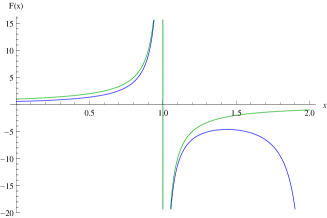
Figure 3: The function $F(x)\;(blue)$ and its approximation $\frac{1}{1-x}\;(green)$.

This corresponds to electrons with energies $\leq c\sqrt{1.5}\sqrt{2\hbar eB}$. Since the spectrum of relativistic Landau levels in graphene is $\epsilon_{n}=\pm v_{F}\sqrt{2n\hbar eB}$ [5], our approximation stays valid up to energies $\sim\sqrt{1.5}\frac{c}{v_{F}}\epsilon_{1}\sim 350\,\epsilon_{1}$, therefore in a domain that largely exceeds the energy $\epsilon_{1}$ of the lowest Landau level .

In practice, this corresponds to electrons with energy $p_{0}\leq 13\sqrt{B(T)}\,eV$. This condition is always satisfied for optical wavelengths; indeed the energy of photons range then between $1.5\,eV$ and $3.5\,eV$, which is roughly twice the energy of the created virtual electrons or positrons.

Notice that, at $x\equiv\frac{p_{0}^{2}}{2eB}=0$, which corresponds to $p_{0}=0$ (electrons with vanishing energy) or to $B\to\infty$, $F(0)=\frac{\ln{3}}{2}\approx.55$ while our approximation goes to $1$. A corresponding scaling down of $\alpha$ can eventually be operated.

We shall therefore take in the following calculations

$$\begin{split}G(\hat{p},B)&\approx-e^{-\frac{p_{1}^{2}+p_{2}^{2}}{eB}}\left[\frac{\gamma^{0}}{p^{0}}\left(1+i\gamma_{1}\gamma_{2}\;\frac{p_{0}^{2}+2eB}{p_{0}^{2}-2eB}\right)-4\frac{p_{1}\gamma_{1}+p_{2}\gamma_{2}}{p_{0}^{2}-2eB}\right],\cr&=-e^{-\frac{p_{1}^{2}+p_{2}^{2}}{eB}}\left[\frac{p^{0}\gamma^{0}}{p_{0}^{2}}(1-i\gamma_{1}\gamma_{2})+2i\frac{p^{0}\gamma^{0}}{p_{0}^{2}-2eB}\gamma_{1}\gamma_{2}-4\frac{p_{1}\gamma_{1}+p_{2}\gamma_{2}}{p_{0}^{2}-2eB}\right],\end{split}$$ (47)

which leads to expressions easy to handle, and enables to go a long way analytically. In particular, setting the momentum along the direction of $B$ equal to $0$ for both electron propagators inside the loop makes their denominators only depend on $p_{0}$. The integration of the transverse degrees of freedom $p_{1},p_{2}$ being elementary, the vacuum polarization can finally be expressed only in terms of 1-dimensional convergent integrals $\int dp_{0}$ (see subsection 4.2.2). In the last line of (47) we have made the distinction between three contributions: the one on the left corresponds to the only term which is usually kept at $B=\infty$ (when $m\not=0$, $p_{3}\not=0$), the middle one and the one on the right are dropped at this same limit. However, in the following, the right contribution will be seen to yield the leading components of the vacuum polarization tensor, due to the powers of $eB$ that arise when integrating over the transverse degrees of freedom $p_{1},p_{2}$ occurring in its numerator.

4.2 Calculations and results

There are two steps in the calculation: first performing the traces of the Dirac $\gamma$ matrices, then integrating over the loop variables $\hat{p}=(p_{0},p_{1},p_{2})$.

4.2.1 Performing the traces of Dirac matrices

This already yields

$$\Pi^{i3}=0=\Pi^{3i},\quad i=0,1,2.$$ (48)

4.2.2 Doing the integrations

Details of the calculation will be given somewhere else. We just want here to present its main steps, taking the examples of $\Pi^{00}$ and $\Pi^{33}$, which play the leading roles in the calculations concerning the refractive index. After doing the traces, one gets

$$\begin{split}iT^{00}(\hat{q},B)&=4\,e^{2}\int_{-\infty}^{+\infty}\frac{dp_{0}dp_{1}dp_{2}}{(2\pi)^{3}}e^{-p_{\perp}^{2}/eB}e^{-(p+q)_{\perp}^{2}/eB}\cr&\left(\frac{1}{p_{0}}\frac{1}{p_{0}+q_{0}}+\frac{1}{p_{0}}\frac{p_{0}^{2}+2eB}{p_{0}^{2}-2eB}\frac{1}{p_{0}+q_{0}}\frac{(p_{0}+q_{0})^{2}+2eB}{(p_{0}+q_{0})^{2}-2eB}+16\frac{p_{1}(p_{1}+q_{1})+p_{2}(p_{2}+q_{2})}{(p_{0}^{2}-2eB)((p_{0}+q_{0})^{2}-2eB)}\right),\end{split}$$ (49)

which decomposes into

$$\begin{split}iT^{00}(\hat{q},B)&=I(\hat{q},B)+J(\hat{q},B)+K(\hat{q},B),\cr I(\hat{q},B)&=4\,e^{2}\int_{-\infty}^{+\infty}\frac{dp_{0}dp_{1}dp_{2}}{(2\pi)^{3}}e^{-p_{\perp}^{2}/eB}e^{-(p+q)_{\perp}^{2}/eB}\frac{1}{p_{0}}\frac{1}{p_{0}+q_{0}},\cr J(\hat{q},B)&=4\,e^{2}\int_{-\infty}^{+\infty}\frac{dp_{0}dp_{1}dp_{2}}{(2\pi)^{3}}e^{-p_{\perp}^{2}/eB}e^{-(p+q)_{\perp}^{2}/eB}\frac{1}{p_{0}}\frac{p_{0}^{2}+2eB}{p_{0}^{2}-2eB}\frac{1}{p_{0}+q_{0}}\frac{(p_{0}+q_{0})^{2}+2eB}{(p_{0}+q_{0})^{2}-2eB},\cr K(\hat{q},B)&=4\,e^{2}\int_{-\infty}^{+\infty}\frac{dp_{0}dp_{1}dp_{2}}{(2\pi)^{3}}e^{-p_{\perp}^{2}/eB}e^{-(p+q)_{\perp}^{2}/eB}16\frac{p_{1}(p_{1}+q_{1})+p_{2}(p_{2}+q_{2})}{(p_{0}^{2}-2eB)((p_{0}+q_{0})^{2}-2eB)}.\end{split}$$ (50)

Likewise, one gets

$$iT^{33}(\hat{q},B)=I(\hat{q},B)+J(\hat{q},B)-K(\hat{q},B).$$ (51)

It is then convenient to integrate over the transverse degrees of freedom $p_{1},p_{2}$. This is done by going to the variables of integration $u_{1}=p_{1}+\frac{q_{1}}{2},u_{2}=p_{2}+\frac{q_{2}}{2}$ and canceling all terms which are odd in $u_{1}$ or $u_{2}$. This yields

$$\begin{split}I(\hat{q},B)&=\frac{\alpha}{\pi}eB\;e^{-q_{\perp}^{2}/2eB}B(q_{0}),\cr J(\hat{q},B)&=\frac{\alpha}{\pi}eB\;e^{-q_{\perp}^{2}/2eB}C(q_{0},B),\cr K(\hat{q},B)&=\frac{8\alpha}{\pi}eB\;e^{-q_{\perp}^{2}/2eB}(eB-q_{\perp}^{2})D(q_{0},B),\end{split}$$ (52)

in which we have introduced the (convergent) integrals

$$\begin{split}B(q_{0})&=\int_{-\infty}^{+\infty}dp_{0}\;\frac{1}{p_{0}}\frac{1}{p_{0}+q_{0}},\cr C(q_{0},B)&=\int_{-\infty}^{+\infty}dp_{0}\;\frac{1}{p_{0}}\frac{p_{0}^{2}+2eB}{p_{0}^{2}-2eB}\frac{1}{p_{0}+q_{0}}\frac{(p_{0}+q_{0})^{2}+2eB}{(p_{0}+q_{0})^{2}-2eB},\cr D(q_{0},B)&=\int_{-\infty}^{+\infty}dp_{0}\;\frac{1}{(p_{0}^{2}-2eB)((p_{0}+q_{0})^{2}-2eB)}.\end{split}$$ (53)

Note that two powers of $eB$ occur in $K$ due to the integration over the transverse degrees of freedom.

“Massless” and ambiguous integrals of the type $\int_{-\infty}^{+\infty}d\sigma\;\frac{f(\sigma)}{\sigma}$ occurring in $B(q_{0}),C(q_{0},B),D(q_{0},B)$ are replaced, using the customary $+i\varepsilon$ prescription for the poles of propagators in QFT dictated by causality, with

$$\lim_{\epsilon\to 0^{+}}\int_{-\infty}^{+\infty}d\sigma\;\frac{f(\sigma)}{\sigma+i\epsilon}=-i\pi\,f(0)+\lim_{\epsilon\to 0^{+}}\int_{|\sigma|>\epsilon}\frac{f(\sigma)}{\sigma},$$ (54)

which are just Cauchy integrals. This is nothing more than the Sokhotski-Plemelj theorem [20] :

$$\lim_{\varepsilon\to 0^{+}}\int_{-\infty}^{\infty}\frac{f(x)}{x\pm i\varepsilon}\,dx=\mp i\pi f(0)+\lim_{\varepsilon\to 0^{+}}\int_{|x|>\varepsilon}\frac{f(x)}{x}\,dx.$$ (55)

It is easy to also check that the same result can be obtained, after setting the $+i\varepsilon$ prescription, by integrating on the contour described on Figure 4. There, the two small 1/2 circles around the poles have radii that $\to 0$. The large 1/2 circle has infinite radius.

Figure 4: The contour of integration for $B(q_{0})$ and $C(q_{0})$.

This also amounts, for the poles “on the real axis”, to evaluating $i\pi\sum residues$, that is $1/2$ of what one would get if the poles were not on the real axis but inside the contour of integration. The other poles that lie inside the contour of integration are dealt with as usual by $2i\pi\times$ their residues.

So doing, one gets

$$\begin{split}&B(q_{0})=0=C(q_{0},B),\cr&D(q_{0},B)=2i\pi(-)\frac{1}{\sqrt{2eB}}\frac{1}{q_{0}^{2}-8eB},\end{split}$$ (56)

leading finally to

$$I=0=J,\quad K(\hat{q},B)=i\frac{2e^{2}}{\pi}\;e^{-\frac{q_{\perp}^{2}}{2eB}}\sqrt{2eB}\;\frac{eB-q_{\perp}^{2}}{q_{0}^{2}-8eB},$$ (57)

and, for $T^{00}(\hat{q},B)$, to the first line of the set of equations (58). From (50), (51) and (57) one gets immediately $T^{33}(\hat{q},B)=-T^{00}(\hat{q},B)$.

Notice that $T^{00}(\hat{q},B)$ and $T^{33}(\hat{q},B)$ are controlled by $K(\hat{q},B)$ which originates from the terms proportional to $4\frac{p_{1}\gamma_{1}+p_{2}\gamma_{2}}{p_{0}^{2}-2eB}$ in the electron propagator (47). These terms are subleading with respect to the ones proportional to $\frac{\gamma^{0}}{p^{0}}(1-i\gamma_{1}\gamma_{2})$ and would have naively been dropped in the limit $B\to\infty$. However, in the calculation of $K(\hat{q},B)$, integrating over the transverse degrees of freedom brings two powers of $eB$ which counter-balances the damping of $D(q_{0},B)$ at large $B$ and finally makes $T^{00}$ and $T^{33}$ the dominant components of the vacuum polarization tensor. Since the powers of $p_{1}$ and $p_{2}$ stay the same, going to higher orders in the expansion at “large $\tau eB$” of the electron propagator would not change the result.

After all integrals have been calculated by similar techniques, one gets the results displayed in subsection 4.2.3.

4.2.3 Explicit expression of $\boldsymbol{T^{\mu\nu}(\hat{q},B)}$ at 1-loop

$$\begin{split}iT^{00}(\hat{q},B)&=4i\alpha\;\sqrt{2eB}\;e^{-\frac{q_{1}^{2}+q_{2}^{2}}{2eB}}\;\frac{2eB-2(q_{1}^{2}+q_{2}^{2})}{q_{0}^{2}-4(2eB)}\stackrel{{\scriptstyle B\to\infty}}{{\simeq}}-i\alpha\;\sqrt{2eB}\;e^{-\frac{q_{1}^{2}+q_{2}^{2}}{2eB}},\cr iT^{11}(\hat{q},B)&=4i\alpha\,e^{-\frac{q_{1}^{2}+q_{2}^{2}}{2eB}}\sqrt{2eB}\,\frac{q_{1}^{2}-q_{2}^{2}}{q_{0}^{2}-4(2eB)}\stackrel{{\scriptstyle B\to\infty}}{{\simeq}}i\alpha\,e^{-\frac{q_{1}^{2}+q_{2}^{2}}{2eB}}\,\frac{q_{1}^{2}-q_{2}^{2}}{\sqrt{2eB}},\cr iT^{22}(\hat{q},B)&=-iT^{11}(\hat{q},B),\quad iT^{33}(\hat{q},B)=-iT^{00}(\hat{q},B),\cr iT^{01}(\hat{q},B)&=2i\alpha\,e^{-\frac{q_{1}^{2}+q_{2}^{2}}{2eB}}q_{1}q_{0}\,\frac{\sqrt{2eB}}{q_{0}^{2}-2eB}\stackrel{{\scriptstyle B\to\infty}}{{\simeq}}-i\alpha\,e^{-\frac{q_{1}^{2}+q_{2}^{2}}{2eB}}\,\frac{q_{1}q_{0}}{\sqrt{2eB}},\cr iT^{02}(\hat{q},B)&=2i\alpha\,e^{-\frac{q_{1}^{2}+q_{2}^{2}}{2eB}}q_{2}q_{0}\,\frac{\sqrt{2eB}}{q_{0}^{2}-2eB}\stackrel{{\scriptstyle B\to\infty}}{{\simeq}}-i\alpha\,e^{-\frac{q_{1}^{2}+q_{2}^{2}}{2eB}}\,\frac{q_{2}q_{0}}{\sqrt{2eB}},\cr iT^{12}(\hat{q},B)&=-16\alpha\,q_{1}q_{2}\,e^{-\frac{q_{1}^{2}+q_{2}^{2}}{2eB}}\frac{\sqrt{2eB}}{q_{0}^{2}-4(2eB)}\stackrel{{\scriptstyle B\to\infty}}{{\simeq}}4\alpha\,e^{-\frac{q_{1}^{2}+q_{2}^{2}}{2eB}}\,\frac{q_{1}q_{2}}{\sqrt{2eB}},\cr iT^{03}(\hat{q},B)&=0,\quad iT^{13}(\hat{q},B)=0,\quad iT^{23}(\hat{q},B)=0.\end{split}$$ (58)

4.2.4 Comments

$\bullet$ $T^{00}=-T^{33}$ are the only two components that do not vanish when $B\to\infty$ (see also footnote 19 concerning $\theta\to 0$).

$\bullet$  $T^{\mu\nu}$ is not transverse. In our setup, which has in particular $q_{2}=0$, the four relations corresponding to $q_{\mu}T^{\mu\nu}(q)$ reduce to

$$q_{\mu}T^{\mu 0}\equiv q_{0}T^{00}+q_{1}T^{10},\quad q_{\mu}T^{\mu 1}\equiv q_{0}T^{01}+q_{1}T^{11},\quad q_{\mu}T^{\mu 2}\equiv 0,\quad q_{\mu}T^{\mu 3}\equiv q_{3}T^{33}.$$ (59)

At the limit $B\to\infty$, they shrink to

$$q_{\mu}T^{\mu 0}\equiv q_{0}T^{00},\quad q_{\mu}T^{\mu 1}\equiv 0,\quad q_{\mu}T^{\mu 2}\equiv 0,\quad q_{\mu}T^{\mu 3}\equiv q_{3}T^{33}.$$ (60)

This non-transversality contrasts with the formula (34) in Tsai-Erber [9] for the general $(3+1)$-dimensional vacuum polarization in an external $B$, which they shown in their eq. (36) to be transverse. It can be traced back to classically setting respectively $p_{3}=0$ and $p_{3}+q_{3}=0$ inside the two propagators of graphene-born electrons, which cannot be achieved without $q_{3}=0$, which makes true the last relation (60). One should however not focus on $T^{\mu\nu}$ because the transversality condition concerns the vacuum polarization $\Pi^{\mu\nu}$, $T^{\mu\nu}$ being only an intermediate step in the calculation. We shall comment more about transversality in subsection 7.3.

5 The light-cone equations and their solutions

5.1 Orders of magnitude

In order to determine inside which domains we have to vary the dimensionless parameters, it is useful to know the orders of magnitude of the physical parameters involved in the study.

$\bullet$ The thickness of graphene is $2a\approx 350\,pm$.

$\bullet$  As stated in (26), $|p_{3}^{max}|\simeq\frac{\hbar}{a}$. This gives $c\,p_{3}^{max}\simeq 1.8\,10^{-16}J$ or $c\,p_{3}^{max}\simeq 1130\,eV\approx 2.2\,10^{-3}\,m_{e}$.

$\bullet$  To $eB$ corresponds $m^{2}=\frac{\hbar eB}{c^{2}}$. For example to $eB^{m}$ (see below) corresponds the mass $\frac{\sqrt{\hbar eB^{m}}}{c}\approx 2\leavevmode\nobreak\ 10^{-33}\,kg\approx 2\leavevmode\nobreak\ 10^{-3}\,m_{e}\ll m_{e}$.

$\bullet$ $[B]=\frac{[p]^{2}}{[e]\hbar}$ such that, to $(p_{3}^{m})^{2}$ corresponds $B^{m}\simeq\frac{\hbar}{ea^{2}}\approx 21400\,T$.

$\bullet$ One has $\zeta\equiv\frac{\sqrt{2e\hbar B}}{p_{3}^{m}}=\sqrt{2\frac{B}{B^{m}}}$. Since $B=\frac{\zeta^{2}}{2}B_{m}$, to $\zeta$ corresponds the mass $\sqrt{2}\,\zeta\,10^{-3}\,m_{e}$.

$\bullet$  We shall consider magnetic fields in the range $[1\,T,20\,T]$;

$$1\,T\leq B\leq 20\,T\Leftrightarrow 1/100\leq\zeta\leq\sqrt{20}/100.$$ (61)

$\bullet$ The wavelength of visible light lies between $350\,nm$ and $700\,nm$, which corresponds to frequencies $\nu$ between $4.3\,10^{14}\,Hz$ and $7.9\,10^{14}\,Hz$, to energies in the range $[3.5\,eV,1.5\,eV]$ and to $\eta=\frac{q_{0}}{cp_{3}^{m}}=\frac{2\pi a\nu}{c}$ such that

$$\text{visible light}\leftrightarrow 1.6\,10^{-3}\leq\eta\leq 2.9\,10^{-3}\ll 1.$$ (62)

5.2 The light-cone equations

It is now straightforward to write the light-cone relations (9) and (10) in the case of graphene. We first express the relevant components $T^{11},T^{22},T^{33}$ in terms of dimensionless variables

$$\begin{split}T^{11}(n,\theta,\eta,\zeta)&=4\alpha\,e^{-(n_{x}^{2}+n_{y}^{2})\frac{\eta^{2}}{\zeta^{2}}}\;\zeta\,\eta^{2}\,p_{3}^{m}\;\frac{n_{x}^{2}-n_{y}^{2}}{\eta^{2}-4\zeta^{2}},\cr T^{22}(n,\theta,\eta,\zeta)&=-T^{11}(\alpha,n,\theta,\eta,\zeta),\cr T^{33}(n,\theta,\eta,\zeta)&=-4\alpha\,e^{-(n_{x}^{2}+n_{y}^{2})\frac{\eta^{2}}{\zeta^{2}}}\;\zeta\,p_{3}^{m}\;\frac{\zeta^{2}-2(n_{x}^{2}+n_{y}^{2})\eta^{2}}{\eta^{2}-4\zeta^{2}},\end{split}$$ (63)

in which $n_{x}=ns_{\theta}$ and, since $q_{2}=0$, $n_{y}=0$ . Then, (9), (10) and (34) lead to

$$\begin{split}&\star\ for\ A^{\mu}_{\perp}:(1-n^{2})\left[1+\frac{p_{3}^{m}}{\pi^{2}}\;\frac{1}{q_{0}^{2}}\;T^{22}(n,\theta,\eta,\zeta)\;V(n,\theta,\eta,u)\right]=0,\cr\;&\star\ for\ A^{\mu}_{\parallel}:(1-n^{2})\left[1+\frac{p_{3}^{m}}{\pi^{2}}\;\frac{1}{q_{0}^{2}}\Big{(}c^{2}_{\theta}\,T^{11}(n,\theta,\eta,\zeta)+s^{2}_{\theta}\,T^{33}(n,\theta,\eta,\zeta)\Big{)}\;V(n,\theta,\eta,u)\right]=0,\end{split}$$ (64)

and, using (63), to

$$\begin{split}&\star\ for\ A^{\mu}_{\perp}:(1-n^{2})\left[1-\frac{4\alpha}{\pi^{2}}\,s_{\theta}^{2}n^{2}\,\frac{\zeta}{\eta^{2}-4\zeta^{2}}\;e^{-(ns_{\theta}\,\frac{\eta}{\zeta})^{2}}\;V(n,\theta,\eta,u)\right]=0,\cr&\star\ for\ A^{\mu}_{\parallel}:(1-n^{2})\left[1+\frac{4\alpha}{\pi^{2}}s_{\theta}^{2}\left(c_{\theta}^{2}n^{2}\,\frac{\zeta}{\eta^{2}-4\zeta^{2}}+\frac{\zeta}{\eta^{2}}\frac{2\eta^{2}n^{2}s_{\theta}^{2}-\zeta^{2}}{\eta^{2}-4\zeta^{2}}\right)\,e^{-(ns_{\theta}\,\frac{\eta}{\zeta})^{2}}\,V(n,\theta,\eta,u)\right]=0.\end{split}$$ (65)

For each polarization, this defines an index $n=n(\alpha,u,\theta,\eta,\zeta)$.

At large values of $\Upsilon\equiv\frac{\zeta}{\eta}$, the second contribution to the light-cone equation for $A^{\mu}_{\parallel}$ inside the $(\ )$, which is that of $T^{33}$, largely dominates.

5.3 Analytical expression for the transmittance $\boldsymbol{V(n,\theta,\eta,u)}$

In order to solve the light-cone equations (65), the first step is to compute $V$, so as to get an algebraic equation for $n$. $V$ as given by (33) is the Fourier transform of the function $x\mapsto-\eta^{2}\frac{\sin x}{x(x-\sigma_{1})(x-\sigma_{2})}$ where

$$\sigma_{1}=-\eta\left(nc_{\theta}-\sqrt{1-n^{2}s_{\theta}^{2}}\right),\quad\sigma_{2}=-\eta\left(nc_{\theta}+\sqrt{1-n^{2}s_{\theta}^{2}}\right)$$ (66)

are the poles of the integrand. The Fourier transform of such a product of a cardinal sine with a rational function is well known. The result involves Heavyside functions of the imaginary parts of the poles $\sigma_{1},\sigma_{2}$, noted $\Theta_{i}^{+}$ for $\Theta_{i}(\Im(\sigma_{i}))$ and $\Theta_{i}^{-}$ for $\Theta_{i}(-\Im(\sigma_{i}))$.

$$\hskip-28.45274ptV(u,n,\theta,\eta)=\frac{-\pi\eta^{2}}{\sigma_{1}\sigma_{2}(\sigma_{1}-\sigma_{2})}\left[(\sigma_{1}-\sigma_{2})+\sigma_{2}\left(\Theta_{1}^{-}e^{-i\sigma_{1}(1-u)}+\Theta_{1}^{+}e^{+i\sigma_{1}(1+u)}\right)-\sigma_{1}\left(\Theta_{2}^{-}e^{-i\sigma_{2}(1-u)}+\Theta_{2}^{+}e^{+i\sigma_{2}(1+u)}\right)\right].$$ (67)

The poles $\sigma_{1},\sigma_{2}$ are seen to control the behavior of $V$, thus of $n$, which depends on the signs of their imaginary parts. That the Fourier transform is well defined needs in particular that the poles have a non-vanishing imaginary part. This requires either $n\not\in{\mathbb{R}}$ or $ns_{\theta}>1$.

The case when the poles are real needs a special treatment. A first possibility is to define the integral as a Cauchy integral, like we did when calculating $T^{\mu\nu}$, arguing in particular of the $+i\varepsilon$ which is understood in the denominator of the outgoing photon propagator. Then, $V$ is calculated through contour integration in the complex plane. This alternate method can also be used when the poles are complex. It is comforting that the two methods give, at leading order in an expansion at small $\eta$ and $n_{2}$ ($n_{2}$ is the imaginary part of the refractive index) the same results. In particular, the cutoff that is then needed to stabilize the integration on the large upper 1/2 circle turns out to be the same as the one that naturally arises in the Fourier transform because of the $\frac{\sin\sigma}{\sigma}$ function. The second, and simplest, possibility, is to define everywhere in (67) $\Theta(0)=\frac{1}{2}$. It is equivalent to the previous one, again at leading order in an expansion at small $\eta$ and $n_{2}$. Then, one gets, at $u=0$ (which is always a very good approximation)

$$V(0,n,\theta,\eta)\stackrel{{\scriptstyle poles\in{\mathbb{R}}}}{{=}}\frac{\pi}{1-n^{2}}\left(1+\frac{\sigma_{2}\cos\sigma_{1}-\sigma_{1}\cos\sigma_{2}}{2\eta\sqrt{1-n^{2}s^{2}_{\theta}}}\right).$$ (68)

Last, if one shrinks $V$ to $\int_{-\infty}^{+\infty}e^{i\sigma u}\frac{\sin\sigma}{\sigma}$, which means only accounting for the gate function in the transmittance, it becomes $V=\pi$ inside graphene (see also subsection 5.4.11).

5.4 Solving the light-cone equations for $\boldsymbol{A^{\mu}_{\parallel}}$ and $\boldsymbol{n\in{\mathbb{R}}>\frac{1}{\sin\theta}}$

That $n\in{\mathbb{R}}$ largely simplifies the equations. No non-trivial solution has been found for $n<\frac{1}{s_{\theta}}$ (see subsection 5.8).

5.4.1 Calculation of $\boldsymbol{V(n,\theta,\eta,u)}$

Expanding $V$ at leading orders in $\eta$, one gets

$$\begin{split}\star\ \Re(V)&=-\frac{\pi}{\sqrt{n^{2}s^{2}_{\theta}-1}}\;\eta+\frac{1}{2}\pi(1+u^{2})\eta^{2}+{\cal O}(\eta^{3}),\cr\star\ \Im(V)&=u\,n\,c_{\theta}\;\frac{\pi}{\sqrt{n^{2}s^{2}_{\theta}-1}}\;\eta^{2}+{\cal O}(\eta^{3}).\end{split}$$ (69)

The expansion for $\Im(V)$ in (69) starts at ${\cal O}(\eta^{2})$ while that of $\Re(V)={\cal O}(\eta)$.

For $n\in{\mathbb{R}}>\frac{1}{s_{\theta}}$, we replace in (66) $\sqrt{1-n^{2}s^{2}_{\theta}}$ with $i\sqrt{n^{2}s^{2}_{\theta}-1}$ and the two poles $\sigma_{1}$ and $\sigma_{2}$ of $V$ become

$$\sigma_{1}=-\eta\left(n\cos\theta-i\sqrt{n^{2}s_{\theta}^{2}-1}\right),\qquad\sigma_{2}=-\eta\left(n\cos\theta+i\sqrt{n^{2}s_{\theta}^{2}-1}\right);$$ (70)

the first term in $\Re(V)$ coincides with $\pm 2i\pi\times$ the residue at the pole $\sigma_{1}$ or $\sigma_{2}$ that lies inside the contour of integration when one calculates $V$ as a contour integral (see (76)).

5.4.2 $\boldsymbol{V}$ at $\boldsymbol{\theta=0}$

At $\theta=0$ the poles $\sigma_{1}=-\eta(n-1),\sigma_{2}=-\eta(n+1)$ are real such that we set $\Theta(0)=\frac{1}{2}$ in the general formula (67). The expression (67) for $V$ becomes

$$V_{\theta=0}=-\frac{\pi\eta^{2}}{\sigma_{1}\sigma_{2}}\left(1+\frac{\sigma_{2}\cos\sigma_{1}\,e^{iu\sigma_{1}}-\sigma_{1}\cos\sigma_{2}\,e^{iu\sigma_{2}}}{\sigma_{1}-\sigma_{2}}\right).$$ (71)

Using the explicit expressions of the poles just written and expanding the $\cos$ and $\exp$ functions at small values of $\sigma_{1},\sigma_{2}$ (we suppose that $n$ is much smaller that its quantum upper limit $n_{quant}\sim\frac{1}{\eta}$ (see subsection 5.6), and that, accordingly, $|\sigma_{1}|,|\sigma_{2}|\ll 1$) one gets finally

$$V_{\theta=0}\approx\frac{\pi\eta^{2}}{2}(1+u^{2}).$$ (72)

It will be used later to show, for $B\not=0$ as well as for $B=0$, that the only solution of the light-cone equations at $\theta=0$ is the trivial $n=1$.

5.4.3 The imaginary parts of the light-cone equations

The imaginary parts of both light-cone equations (65) shrink, for $n$ real, to

$$\Im(V)=0.$$ (73)

It is only rigorously satisfied at $u=0$, but, (69) and numerical calculations show that, for values of $\eta$ in the visible spectrum $\eta\in[1.6/1000,2.9/1000]$, $\Im(V)\ll\Re(V)<1$ and that $\Im(V)\approx 0$ is always an excellent approximation.

5.4.4 There is no non-trivial solution for $\boldsymbol{A^{\mu}_{\perp}}$

Detailed numerical investigations show that no solution exists for the transverse polarization but the trivial solution $n=1$. We shall therefore from now onwards only be concerned with photons $A^{\mu}_{\parallel}$ with a parallel polarization (see Figure 1).

5.4.5 The light-cone equation for $\boldsymbol{A_{\parallel}^{\mu}}$ and its solution

Expanding $V$ in powers of $\eta$ and neglecting $\Im(V)$ enables to get, through standard manipulations, a simple analytical equation for the refractive index $n$. For $\Upsilon\equiv\frac{\sqrt{2eB}}{q_{0}}\gg 1$ and $\eta<3/1000$, the following accurate expression is obtained by expanding (65) in powers of $\frac{1}{\Upsilon}$

$$(1-n^{2})\left[1-\frac{\alpha}{\pi}\Upsilon\;\frac{s^{2}_{\theta}}{\sqrt{n^{2}s^{2}_{\theta}-1}}\left(1+\frac{-3n^{2}s^{2}_{\theta}-c^{2}_{\theta}+1/4}{\Upsilon^{2}}\right)\right]=0,$$ (74)

which leads consistently to the non-trivial solution of the light-cone equation (65)

$$n^{2}\simeq\frac{1}{s_{\theta}^{2}}\ \frac{1+\left(\frac{\alpha\Upsilon s_{\theta}^{2}}{\pi}\right)^{2}\left(1+\frac{1}{2\Upsilon^{2}}\right)}{1+2\left(\frac{\alpha s_{\theta}}{\pi}\right)^{2}(3s_{\theta}^{2}+c_{\theta}^{2})}.$$ (75)

5.4.6 Graphical results and comments

The results given in eq. (75) are plotted on Figure 5. On the left we vary $\alpha$ from $\frac{1}{137}$ to $2$ at $\Upsilon=10$ and on the right we keep $\alpha=1$ and vary $\Upsilon$ between $5$ and $20$. On both plots, the black lower curve is $n=\frac{1}{\sin\theta}$ (on the left plot it cannot be distinguished from the blue curve). We have shaded the domain of low $\theta$ in which $n$ must make a transition to another regime (see subsection 5.5).

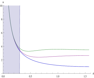
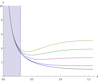
Figure 5: The index $n\in{\mathbb{R}}$ for $A^{\mu}_{\parallel}$ as a function of $\theta$. On the left we vary $\alpha=1/137\,(blue),1\,(purple),2\,(green)$ at $\Upsilon=10$; on the right we vary $\Upsilon=5\,(blue),10\,(purple),15\,(green),20\,(yellow)$ at $\alpha=1$. The lower (black) curves are $1/\sin\theta$.

$\star$ The curves go asymptotically to $\frac{1}{s_{\theta}}$ when $\theta\to 0$. However, we shall see that they should be truncated before $\theta=0$).

$\star$ At large angles, the effects are mainly of quantum nature, strongly influenced by the presence of $B$ and largely depending on the value of $\alpha$; when $\theta$ gets smaller, one goes to another regime in which the effects of confinement are the dominant ones.

1-loop effects are therefore potentially large at $\alpha\geq 1$. Furthermore, at reasonable values of $B$ and for photons in the visible spectrum, the dependence on $B$ is strong.

$\star$ They increase with $\Upsilon=\frac{c\sqrt{2\hbar eB}}{q_{0}}$, therefore inversely to the energy of the photon : low frequencies are favored for testing, and this limit is fortunate since our expansions are done at $\eta=aq_{0}(/\hbar c)\ll 1$. As for the proportionality to $\sqrt{eB}$ for very large values of $eB$, it should be compared with the corresponding factor $eB$ pointed at in [4] in the “vacuum”. The difference in powers can be easily traced back to the different integrations in the course of the calculations. In our case, integrating over the transverse electronic degrees of freedom yields a factor $(eB)^{2}$ while the remaining integral $D$ (53) over $p_{0}$ yields a factor $1/(eB)^{3/2}$. This apparently infinitely growing refraction with $eB$ should however stop at $B=B^{m}$, above which new quantum effects are expected (see subsection 5.6).

$\star$ For $\eta\ll 1$ and $n>\frac{1}{s_{\theta}}$, the residues of $V$ at the poles $\sigma_{1}$ and $\sigma_{2}$ are

$$res(\sigma_{1})=-\frac{\eta}{2i\sqrt{n^{2}s^{2}_{\theta}-1}}+{\cal O}(\eta^{2})=-res(\sigma_{2}).$$ (76)

The agreement between $\Re(V)$ in the first line of (69) and $\pm 2i\pi\ res(\sigma_{1})$ is conspicuous. Indeed, it is easy to prove that for $n\in{\mathbb{R}}$, only one of the two poles lies inside the contour of integration in the upper 1/2 complex $\sigma$-plane, which is the alternate method to calculate $V$.

$\star$ In the approximation that we made, the refractive index does not depends on $u$, the position inside the strip. This dependence, very weak, only starts to appear through higher orders in the expansion of the transmittance $U$ (or $V$).

$\star$ $n$ does not depend explicitly on the thickness $a$ (it depends only on $\Upsilon$, independent of $a$). The limit $a\to 0$ (which is compatible with $\eta=aq_{0}\ll 1$) is therefore “smooth” (see also subsection 5.4.8). At the opposite, the limit $a\to\infty$, which corresponds to forgetting about the confinement of vertices and about the transmittance, to exact photon momentum conservation $(k_{3}=0)$ cannot be taken reliably because it is in contradiction with $\eta\ll 1$.

5.4.7 The “leading” $\boldsymbol{n\sim\frac{1}{\sin\theta}}$ behavior

It is easy to track the origin of the leading $\frac{1}{s_{\theta}}$ behavior of the index (we shall see below that the related divergence at $\theta\to 0$ is fake). It comes in the regime when the two poles of $V$ lie in different 1/2 planes, such that $V$ can be safely approximated by $V\approx 2i\pi\times residue(\sigma_{1}\ or\ \sigma_{2})$.

Keeping only the leading terms $\propto\Pi^{33}$ in the light-cone equation (10) and using (34) yields (we factor out $(1-n^{2})$ and forget about the trivial solution $n=1$)

$$1+\frac{s_{\theta}^{2}}{\pi^{2}}\frac{p_{3}^{m}}{q_{0}^{2}}\;T^{33}\,V=0.$$ (77)

Using (76) gives then

$$1-\frac{\alpha s^{2}_{\theta}}{\pi^{2}}\frac{\Upsilon}{\eta}\left(2i\pi\frac{\eta}{2i\sqrt{n^{2}s^{2}_{\theta}-1}}\right)=0.$$ (78)

The factor $\frac{\alpha s^{2}_{\theta}}{\pi^{2}}\frac{\Upsilon}{\eta}$, which depends in particular of $\alpha$ and $B$, originates from $\frac{s_{\theta}^{2}}{\pi^{2}}\frac{p_{3}^{m}}{q_{0}^{2}}T^{33}$ in (77), while the term inside $(\quad)$ comes from the (residue of the) pole of $V$. Eq. (78) yields

$$n^{2}s^{2}_{\theta}-1=\left(\frac{\alpha s^{2}_{\theta}\Upsilon}{\pi}\right)^{2},$$ (79)

in which we recognize the leading terms of the solution (75).

5.4.8 The limit $\boldsymbol{a\to 0}$

At this stage, we can understand why the limit of infinitely thin graphene $a\to 0$ is delicate and should not, a priori, be taken from the start.

Since $\Upsilon$ is independent of $a$, so is eq. (79) . However, this property arises after the cancellation of two $\eta$ factors in (78), one coming from $\frac{p_{3}^{m}}{q_{0}^{2}}T^{33}$ and the second from the residue (76) of $V$. Taking $a=0$ cancels the transmittance $V$ and its poles, such that the $\sqrt{n^{2}s^{2}_{\theta}-1}$ in (78), which yields the l.h.s. of (79) and the leading $1/s_{\theta}$ behavior of $n$, fades away. Notice however that, in the domain of (fairly large) values of $\theta$ in which our results are reliable, this leading behavior is not very constraining, specially at large values of $\alpha$ and $B$.

5.4.9 The trivial solution $\boldsymbol{n=1}$

To better understand the fate of the solution $n=1$, let us rewrite (67) as

$$V(u,n,\theta,\eta)=\frac{\pi}{1-n^{2}}\left[1+\frac{\sigma_{2}\left(\Theta_{1}^{-}e^{-i\sigma_{1}(1-u)}+\Theta_{1}^{+}e^{+i\sigma_{1}(1+u)}\right)-\sigma_{1}\left(\Theta_{2}^{-}e^{-i\sigma_{2}(1-u)}+\Theta_{2}^{+}e^{+i\sigma_{2}(1+u)}\right)}{2\eta\sqrt{1-n^{2}s^{2}_{\theta}}}\right],$$ (80)

in which we have also used the expressions (66) of $\sigma_{1}$ and $\sigma_{2}$. At $n=+1$, $\sigma_{1}=0,\,\sigma_{2}=-2\eta c_{\theta}$ and, at $n=-1$, $\sigma_{1}=2\eta c_{\theta},\,\sigma_{2}=0$ such that, in both cases (80) writes (setting to $\frac{1}{2}$ the two appropriate $\Theta$ functions since the poles are real)

$$V(u,\pm 1,\theta,\eta)=\frac{\pi}{1-n^{2}}\times(1-1).$$ (81)

Accordingly, the product $(1-n^{2})\times V$ occurring in the light-cone equations (65) vanishes for $n=\pm 1$ such that, in particular, the trivial solution $n=1$ always stays valid.

5.4.10 The limit $\boldsymbol{\alpha=0}$

At $\alpha=0$ the contribution of the vacuum polarization vanishes and, as is seen on (74), the only solution is the trivial $n=1$.

To be complete, this limit should also operate smoothly on the nontrivial solution (75). However, since (75) was obtained by the expansion (see subsection 4.1.2) of $tanh(\tau eB)$ and $cosh(\tau eB)$ at large values of their argument (large $B<\infty$), like the limit $B\to 0$, the limit $e\to 0$ cannot be safely obtained in this framework. In particular the apparent limit $n\stackrel{{\scriptstyle\alpha\to 0}}{{\to}}\frac{1}{s_{\theta}}$ that occurs in (75) should be considered as fake.

5.4.11 Shrinking the transmittance to the sole gate function

To test the importance of the poles in the integrand of the transmittance (30) (33), it is instructive to arbitrarily shrink $V$ to the pure geometric (Fourier transform of the) gate function. This drastic approximation forgets about the ratio of external photon propagators at $k_{3}=0$ and $k_{3}\not=0$. One gets then $V=\pi$ inside graphene and the light-cone equation (65) for $A^{\mu}_{\parallel}$ shrinks to (we forget about the global factor $(n^{2}-1)$ and the trivial solution $n=1$)

$$1+\frac{\alpha}{\pi}\frac{s_{\theta}^{2}}{\eta}e^{-\frac{n^{2}s_{\theta}^{2}}{\Upsilon^{2}}}\left(\Upsilon-\frac{n^{2}(1+s_{\theta}^{2})}{\Upsilon}\right)=0.$$ (82)

Eq. (82) has only real solutions and, accordingly, no absorption.

Results are summarized on Figure 6. On the left plots, we keep $\Upsilon=10,\eta=\frac{2}{1000}$ and vary
$\alpha=1/137\,(blue),1/50\,(brown),1/10\,(purple),1\,(yellow),2\,(green)$. On the right, we keep $\alpha=1,\eta=\frac{2}{1000}$ and vary $\Upsilon=5\,(blue),10\,(purple),15\,(green),20\,(yellow)$. The black curves on both figures are $n=\frac{1}{s_{\theta}}$.

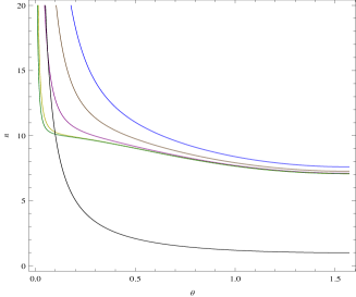
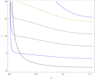
Figure 6: The index $n$ for $A^{\mu}_{\parallel}$ as a function of $\theta$ in the approximation $V=\pi$ inside graphene (gate function). On the left we vary $\alpha=1/137\,(blue),1/50\,(brown),1/10\,(purple),1\,(yellow),2\,(green)$ at $\Upsilon=10,\eta=\frac{2}{1000}$; on the right we vary $\Upsilon=5\,(blue),10\,(purple),15\,(green),20\,(yellow)$ at $\alpha=1$. The lower (black) curves are $1/\sin\theta$.

Like when using the full expression for $V$, the limit of small $\theta$ is not reliable (in particular, a smooth transition to $n=1$ at $\theta=0$ looks more unreachable than ever). In general, $n$ roughly grows like $\Upsilon$ and the role of $\alpha$ has decreased, in particular at large values of $\theta$.

There exist other families of solutions at larger values of $n$. A trace of them can be seen for $\Upsilon=5$ (blue) in the upper 1/2 of the right plot in Figure 6. They are due to the presence of the exponential $e^{n^{2}s_{\theta}^{2}/\Upsilon^{2}}$ in (82).

The large differences that we get with respect to the full calculation shows the importance of treating the transmittance as a complex function of a complex $n$ and of paying special attention to its poles (in close relation with the fluctuations of electron momentum due to the confinement of vertices).

5.5 The transition $\boldsymbol{\theta\to 0}$

5.5.1 At $\boldsymbol{\theta=0}$

The simplest is to come back to the light-cone equation (8). At $\theta=0$ $V$ is given by (72) and, at this same limit, $\Pi^{11}=-\Pi^{22}=0$ since not only $q_{2}=0$ by the choice of frame, but also, now, $q_{1}\equiv|\vec{q}|s_{\theta}=0$. The light-cone equation shrinks then to

$$(\beta_{1}^{2}+\beta_{2}^{2})q^{2}=0,$$ (83)

which has for unique solution the trivial $n=1$.

5.5.2 A cumbersome transition

It is fairly easy to determine the value of $\theta$ below which our calculations and the resulting approximate formula (75) may not be trusted anymore. There presumably starts a transition to another regime.

Our calculations stay valid as long as the two poles $\sigma_{1}$ and $\sigma_{2}$ of the transmittance function $V$ lie in different 1/2 planes. This requires that their imaginary parts have opposite signs. Their explicit expressions are given in (101) below. It is then straightforward to get the following condition (we slightly anticipate and consider $n=n_{1}+in_{2}\in{\mathbb{C}}$)

$$\sigma_{1}\ \text{and}\ \sigma_{2}\ \text{in different 1/2 planes}\Leftrightarrow n_{1}^{2}>\frac{1+n_{2}^{2}}{\tan^{2}\theta}.$$ (84)

(84) is always satisfied at $\theta=\frac{\pi}{2}$ and never at $\theta=0$. Since $n_{2}\approx 0$, the transition occurs at

$$n_{1}(\theta)\approx n(\theta)\approx\frac{1}{\tan\theta},$$ (85)

in which we can use (75) for $n$. Since at small $\theta$, $\sin\theta\simeq\theta\simeq\tan\theta$, this condition writes approximately

$$1\leq\frac{1+\left(\frac{\alpha\Upsilon s_{\theta}^{2}}{\pi}\right)^{2}\left(1+\frac{1}{2\Upsilon^{2}}\right)}{1+2\left(\frac{\alpha s_{\theta}}{\pi}\right)^{2}(3s^{2}_{\theta}+c^{2}_{\theta})}\Leftrightarrow\theta\geq\theta_{min}=\sqrt{\frac{2}{\Upsilon^{2}-\frac{7}{2}}}.$$ (86)

For example, at $\Upsilon=5$ it yields $\theta\geq.3$. Notice that the condition (86) also sets a lower limit $\Upsilon>\sqrt{\frac{7}{2}}$.

It is easy to get the value $n_{max}$ of $n$ at $\theta=\theta_{min}\simeq\frac{\sqrt{2}}{\Upsilon}$ given by (86). Plugging this value in (75) one gets

$$n_{max}\equiv n(\theta=\theta_{min})\approx\frac{\Upsilon}{\sqrt{2}}.$$ (87)

Seemingly, the solution (75) that we have exhibited gets closer and closer to the “leading” $\frac{1}{s_{\theta}}$ when $\theta$ becomes smaller and smaller. It is however easy to show that this divergence is fake, by using our result $n=1$ at $\theta=0$ deduced in subsection 5.5.1.

The diverging solution (75) cannot be trusted down to $\theta=0$ at which $n=1$; so, the true solution of the light-cone equation must cross the curve $n=\frac{1}{s_{\theta}}$ somewhere at small $\theta$. However, such a transition cannot exist. This is most easily proved by showing that, at no value of $\theta$, $n=\frac{1}{s_{\theta}}$ can be a solution to the light-cone equation (65). Let us write $\sigma_{1}=-\eta\frac{c_{\theta}}{s_{\theta}}+\epsilon,\sigma_{2}=-\eta\frac{c_{\theta}}{s_{\theta}}-\epsilon$. The poles being real, $V$ can be calculated by setting $\Theta(0)=\frac{1}{2}$ in (67), which yields

$$\begin{split}V&\stackrel{{\scriptstyle real\ poles}}{{\rightarrow}}-\frac{\pi\eta^{2}}{\sigma_{1}\sigma_{2}(\sigma_{1}-\sigma_{2})}\left(\sigma_{1}-\sigma_{2}+\sigma_{2}\cos\sigma_{1}e^{i\sigma_{1}u}-\sigma_{1}\cos\sigma_{2}e^{i\sigma_{2}u}\right)\cr&\hskip-28.45274pt=-\frac{\pi\eta^{2}}{\sigma_{1}\sigma_{2}(\sigma_{1}-\sigma_{2})}\Big{(}\sigma_{1}-\sigma_{2}+\sigma_{2}\cos\sigma_{1}\cos u\sigma_{1}-\sigma_{1}\cos\sigma_{2}\cos u\sigma_{2}+i\big{(}\sigma_{2}\cos\sigma_{1}\sin u\sigma_{1}-\sigma_{1}\cos\sigma_{2}\sin u\sigma_{2}\big{)}\Big{)}.\end{split}$$ (88)

and, in our case, at $u=0$,

$$V(u=0)\approx-\pi\frac{s^{2}_{\theta}}{c^{2}_{\theta}}\left(1-\cos\Big{(}\eta^{2}\frac{c^{2}_{\theta}}{s^{2}_{\theta}}\Big{)}-\eta\frac{c_{\theta}}{s_{\theta}}\sin\Big{(}\eta\frac{c_{\theta}}{s_{\theta}}\Big{)}\right).$$ (89)

The light-cone equation (65) for $A^{\mu}_{\parallel}$ writes then

$$\left(1-\frac{1}{s^{2}_{\theta}}\right)\left[1+\frac{\alpha}{\pi}\frac{s^{2}_{\theta}}{c^{2}_{\theta}}\frac{1}{\zeta}\left(c^{2}_{\theta}-\Upsilon^{2}s^{2}_{\theta}\Big{(}1-\frac{2}{\Upsilon^{2}}\Big{)}\right)\left(1-\cos\Big{(}\eta^{2}\frac{c^{2}_{\theta}}{s^{2}_{\theta}}\Big{)}-\eta\frac{c_{\theta}}{s_{\theta}}\sin\Big{(}\eta\frac{c_{\theta}}{s_{\theta}}\Big{)}\right)\right]=0,$$ (90)

in which we have incorporated the “trivial” term $(1-n^{2})$.

Eq. (90) has no solution: therefore the crossing that would make the connection between our diverging solution and $n=1$ at $\theta=0$ cannot be realized . This proves that the domain in which we can trust our solution (75) cannot be extended down to $\theta=0$ .

This investigation is continued in subsection 5.7.2 for $n\in{\mathbb{C}}$ (see also subsection 7.2).

5.6 The quantum upper bound $\boldsymbol{n<n_{quant}}$. The threshold at $\boldsymbol{B=B^{m}}$

Quantum Mechanics sets an upper bound $n_{quant}$ for the index. It comes from a constraint that exists on the poles of the outgoing photon propagator, which are also those of the transmittance $U$ : $|k_{3}|$, the momentum exchanged with electrons along $B$ must be smaller or equal to $\frac{\hbar}{a}=p_{3}^{m}$, the cutoff of the (quantum) momentum of the graphene-born electrons along $z$. This translates for the poles (66) of $V$ into

$$|\sigma_{1}|\leq 1,\quad|\sigma_{2}|\leq 1.$$ (91)

For $n\in{\mathbb{R}}>\frac{1}{s_{\theta}}$, both conditions yield

$$n^{2}\leq n^{2}_{quant}=\frac{1}{\eta^{2}}+1.$$ (92)

The existence of this bound is another clue showing that the index cannot diverge at small values of $\theta$, which shrinks the domain of reliability of the solution (75).

At the values of $\eta$ and $\Upsilon$ that we are operating at (see subsection 5.1), $n_{max}$ given in (87) is much smaller than the quantum limit (92). However, when the energy of photons $q_{0}=\frac{\eta}{a}$ increases, $n_{quant}$ decreases, its asymptotic value being $1$ for infinitely energetic photons.

The case $\theta=0$ is special and is investigated directly. One has then $\sigma_{1}=-\eta(n-1),\sigma_{2}=-\eta(n+1)$, such that $|\sigma_{1}|,|\sigma_{2}|\leq 1$, that is

$$|n(\theta=0)|\stackrel{{\scriptstyle quantum}}{{\leq}}\frac{1}{\eta}-1.$$ (93)

To be compatible with $n=1$ at $\theta=0$ that we deduced in subsection 5.5.1, the bound (93) requires $\eta\leq\frac{1}{2}$.

When $B$ and $\Upsilon\equiv c\frac{\sqrt{2\hbar eB}}{q_{0}}$ increase, $\theta_{min}$ given in (86) decreases, while $n_{max}\equiv n(\theta_{min})$ given by (87) increases. A point can be reached at which $n_{max}$ becomes equal to $n_{quant}$; it occurs at $\eta\simeq\frac{\sqrt{2}}{\Upsilon}\Leftrightarrow\zeta\simeq\sqrt{2}$, independently of $\eta$, which corresponds (see subsection 5.1) to $B\simeq B^{m}\approx 21400\,T$. This gives a physical meaning to $B^{m}$, which appears as the (very large) magnetic field at which the two upper bounds $n_{max}$ and $n_{quant}$ coincide. Still increasing $B$ would result in $n_{max}$ exceeding the quantum limit. Beyond this limit, new phenomena are expected which lie beyond the scope of this work.

5.7 Going to $\boldsymbol{n\in{\mathbb{C}}}$

5.7.1 The case of $\boldsymbol{A^{\mu}_{\parallel}}$

Numerical calculations can be performed in the general case of a complex index $n=n_{1}+in_{2}$. They show in particular that $|n_{2}|\ll n_{1}$, confirming the reliability of the approximation that we made in the main stream of this study (we have limited them to values of $\theta$ large enough for our equations to be valid). The results are displayed on Figure 7, in which we plot $n_{2}$ as a function of $\theta$, varying $\alpha$ (left) and $\Upsilon$ (right), and on Figure 8 in which we plot $n_{2}$ as a function of $u$, varying $\Upsilon$.

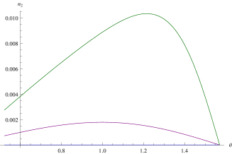
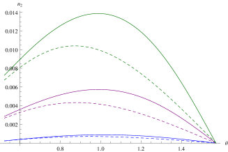
Figure 7: The imaginary part $n_{2}$ of the index $n$ for $A^{\mu}_{\parallel}$ as a function of $\theta$. On the left we vary $\alpha=1/137\,(blue)$, $1\,(purple)$, $2\,(green)$ at $\Upsilon=5$; on the right we vary $\Upsilon=4\,(blue)$, $8\,(purple)$, $12\,(green)$ at $\alpha=1$. The dashed curves on the right correspond to the rough approximation (96).

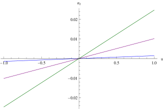
Figure 8: The imaginary part $n_{2}$ of index $n$ for $A^{\mu}_{\parallel}$ as a function of $u$. We take $\alpha=1$, $\eta=5/1000$, and vary $\Upsilon=4\,(blue),8\,(purple),12\,(green)$.

To this purpose, and because the real part of the light-cone equation only gets very slightly modified, it is enough to consider the imaginary part of the light-cone equation (65) for $A^{\mu}_{\parallel}$ in which we plug, for $n_{1}^{2}$, the analytic expression (75). In practice, the expansion of this equation at ${\cal O}(\eta^{2})$ and ${\cal O}(n_{2})$, which is a polynomial of first order in $n_{2}$ is enough for our purposes An important ingredient of the calculation is the expansion of the transmittance $V$ at order ${\cal O}(\eta^{2})$ and ${\cal O}(n_{2})$, in the case when its two poles lie in different 1/2 planes, which writes

$$\begin{split}\star\ \frac{1}{\pi}\Re(V)&=-\frac{\eta}{\sqrt{n_{1}^{2}s^{2}_{\theta}-1}}+\frac{1}{2}(1+u^{2})\eta^{2}+\frac{uc_{\theta}(2n_{1}^{2}s^{2}_{\theta}-1)}{(n_{1}^{2}s^{2}_{\theta}-1)^{\frac{3}{2}}}\eta^{2}n_{2}+\ldots,\cr\star\ \frac{1}{\pi}\Im(V)&=\frac{un_{1}c_{\theta}}{\sqrt{n_{1}^{2}s^{2}_{\theta}-1}}\eta^{2}-\frac{n_{1}s^{2}_{\theta}}{(n_{1}^{2}s^{2}_{\theta}-1)^{\frac{3}{2}}}\eta n_{2}+\ldots\end{split}$$ (94)

The corresponding analytical expression for $n_{2}$, an odd function of $u$, is long and unaesthetic and we only give it in footnote 24 . However a rough order of magnitude can be obtained with very drastic approximations which lead to the equation

$$n_{2}s^{2}_{\theta}\sim u\eta c_{\theta}(n_{1}^{2}s_{\theta}^{2}-1),$$ (96)

in which, like before, we can plug in the analytical formula (75) for $n_{1}^{2}$. The corresponding curves are the dashed ones in Figure 7. The agreement with the exact curves worsens as $\alpha$ increases.

As $B$ increases, it is no longer a reliable approximation to consider $n\in{\mathbb{R}}$ : absorption becomes non-negligible. The window of medium-strong $B$’s from 1 to 20 T together with photons in the visible range appears therefore quite simple and special. Outside this window, the physics is most probably more involved and equations much harder to solve.

5.7.2 The “wall” for $\boldsymbol{A^{\mu}_{\parallel}}$

The situation is best described in the complex $(n_{1},n_{2})$ plane of the solutions $n=n_{1}+in_{2}$ of the light-cone equation (65) for $A^{\mu}_{\parallel}$. In the limit $\eta\ll\zeta\Leftrightarrow\Upsilon\gg 1$, and neglecting the exponential $e^{-\frac{n^{2}s^{2}_{\theta}}{\Upsilon^{2}}}$ which plays a negligible role, it decomposes into its real and imaginary parts according to

$$\begin{split}&\ast\ 1+\frac{\alpha}{\pi}\frac{s^{2}_{\theta}}{\zeta}\left(1+\frac{1}{4\Upsilon^{2}}\right)\left[\left(\Upsilon^{2}-(n_{1}^{2}-n_{2}^{2})(1+s^{2}_{\theta})\right)\Re(V)+2n_{1}n_{2}(1+s^{2}_{\theta})\Im(V)\right]=0,\cr&\ast\ -2n_{1}n_{2}(1+s^{2}_{\theta})\Re(V)+\left(\Upsilon^{2}-(n_{1}^{2}-n_{2}^{2})(1+s^{2}_{\theta}\right)\Im(V)=0.\end{split}$$ (97)

All previous calculations favoring solutions with low absorption $|n_{2}|\ll n_{1}$, it is in this regime that we shall investigate the presence of a “wall” at small $\theta$. To this purpose, we shall plug into the light-cone equation (65) for $A^{\mu}_{\parallel}$ the expansion of the transmittance $V$ that is written in (94).

The situation at $\theta=\frac{\pi}{4}$ (left) and $\theta=\frac{\pi}{10}$ are depicted in Figure 9. The values of the parameters are $\alpha=1,u=.5,\eta=\frac{5}{1000},\Upsilon=5$.

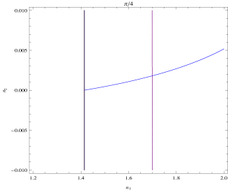
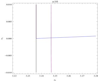
Figure 9: The index $(n_{1},n_{2})$ for $A^{\mu}_{\parallel}$ at $\theta=\frac{\pi}{4}$ (left) and $\theta=\frac{\pi}{10}$ (right).

The purple curve corresponds to the solutions of the real part of the light-cone equation and the blue quasi-vertical line to the solution of its real part. The intersection of the two curves yields the solution $n=n_{1}+in_{2}$. We recover $|n_{2}|\ll n_{1}$. The black vertical line on the left corresponds to $n_{1}=\frac{1}{s_{\theta}}$.

A transition brutally occurs close to $\theta=\frac{\pi}{14}$. Then the solution at $|n_{2}|\ll n_{1}={\cal O}(1)$ disappears. It is clearly visible on Figure 10 below in which we plot the situation after the transition, for $\theta=\frac{\pi}{17}$.

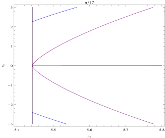
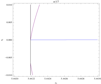
Figure 10: The index $(n_{1},n_{2})$ for $A^{\mu}_{\parallel}$ at $\theta=\frac{\pi}{17}$. The figure on the right is an enlargement of that on the left.

There is no more intersection between the solutions of the real (purple) and imaginary (blue) parts of the light-cone equations, except at $n_{2}=0,n_{1}=\frac{1}{s_{\theta}}$, which is a fake solution since we know that $n_{1}$ can never reach its “asymptotic” value $\frac{1}{s_{\theta}}$.

5.7.3 An estimate of the angle of transition $\boldsymbol{\theta_{min}}$

This change of regime is characterized by a brutal jump in the value of $n_{2}$, which should be manifest on the imaginary part of the light-cone equation (97). A very reliable approximation can be obtained by truncating $\Re(V)$ to its first term, in which case one gets

$$n_{2}\approx(n_{1}^{2}s^{2}_{\theta}-1)\frac{u\eta c_{\theta}\left(\Upsilon^{2}-n_{1}^{2}(1+s^{2}_{\theta})\right)}{s^{2}_{\theta}\left(\Upsilon^{2}-n_{1}^{2}(1+s^{2}_{\theta})\right)-2(1+s^{2}_{\theta})(n_{1}^{2}s^{2}_{\theta}-1)}$$ (98)

which has a pole at (we use $s^{2}_{\theta}\ll 1$)

$$n_{1}^{2}\approx\frac{2+\Upsilon^{2}s^{2}_{\theta}}{3s^{2}_{\theta}}.$$ (99)

This value for $n_{1}$ determines the maximum that can be reached when $\theta$ decreases. Indeed, then, $n_{2}$ becomes out of control in the framework of our approximations. We also know that that $n_{1}$ should stay below $\frac{1}{s_{\theta}}$. The intersection of (99) and $\frac{1}{s_{\theta}}$ yields the lower limit for $\theta$

$$\theta_{min}\sim\frac{1}{\Upsilon}.$$ (100)

(100) is smaller than our previous estimate (86) obtained in the approximation $n\in{\mathbb{R}}$.

At $\Upsilon=5$ one gets $\theta_{min}\approx\frac{\pi}{15}$, which shows the reliability of our estimate (the true transition numerically occurs between $\frac{\pi}{14}$ and $\frac{\pi}{15}$).

5.7.4 The case of $\boldsymbol{A^{\mu}_{\perp}}$

We only summarize below the steps that lead to the conclusion that no solution to the refractive index except the trivial $n=1$ exists for the transverse polarization.

Starting from the corresponding light-cone equation in (65), the main task is to get the appropriate expression for the transmittance function $V$. To this purpose the starting point is the general expression (67). We expand it in powers of $\eta$ in the sense that the exponentials are expanded at ${\cal O}(\eta)$ or, eventually ${\cal O}(\eta^{2})$. No expansion in powers of $n_{2}$ is done because, if solutions exist, they may occur for fairly larges values of $n_{2}$ (and $n_{1}$).

Since the sign of the imaginary parts of the poles $\sigma_{1}$ and $\sigma_{2}$ obviously play a central role, it is also useful to extract ($c$ should not be confused here with the speed of light)

$$\begin{split}\Im(\sigma_{1})&=\eta\left(-n_{2}c_{\theta}+\frac{1}{\sqrt{2}}\sqrt{-c+\sqrt{c^{2}+d^{2}}}\right),\cr\Im(\sigma_{2})&=\eta\left(-n_{2}c_{\theta}-\frac{1}{\sqrt{2}}\sqrt{-c+\sqrt{c^{2}+d^{2}}}\right),\cr c&=1-(n_{1}^{2}-n_{2}^{2})s^{2}_{\theta},\quad d=2n_{1}n_{2}s^{2}_{\theta}.\end{split}$$ (101)

Straightforward manipulations on (67) show that:

* when $n_{2}>0$ ($\Rightarrow\Im(\sigma_{2})<0$): if $\Im(\sigma_{1})>0$, $V=\frac{-i\pi\eta}{\sqrt{1-n^{2}s^{2}_{\theta}}}+\ldots$; if $\Im(\sigma_{1})<0$, $V=\frac{\pi\eta^{2}}{2}(1-u)^{2}+\ldots$
* when $n_{2}<0$ ($\Rightarrow\Im(\sigma_{1})>0$): if $\Im(\sigma_{2})>0$, $V=\frac{\pi\eta^{2}}{2}(1+u)^{2}+\ldots$; if $\Im(\sigma_{2})<0$, $V=\frac{-i\pi\eta}{\sqrt{1-n^{2}s^{2}_{\theta}}}+\ldots$

The cases when $V={\cal O}(\eta^{2})$ correspond to $\sigma_{1}$ and $\sigma_{2}$ being in the same 1/2 complex $\sigma$-plane.

When $V=\frac{-i\pi\eta}{\sqrt{1-n^{2}s^{2}_{\theta}}}$, its real and imaginary parts are given by

$$\Re(V)=\frac{\pi\,\eta\,n_{1}n_{2}\,s^{2}_{\theta}}{\sqrt{2}}\frac{\sqrt{c+\sqrt{c^{2}+d^{2}}}}{\sqrt{c^{2}+d^{2}}},\qquad\Im(V)=\frac{-\pi\,\eta}{\sqrt{2}}\frac{\sqrt{-c+\sqrt{c^{2}+d^{2}}}}{\sqrt{c^{2}+d^{2}}}.$$ (102)

Numerical solutions of the light-cone equation show that no solution exists that fulfill the appropriate criteria on the signs of $\Im(\sigma_{1}),\Im(\sigma_{2})$. For example, for $n_{2}<0$, one gets solutions shared by both the real and imaginary parts of the light-cone equations, but they satisfy $\Im(\sigma_{2})>0$ and must therefore be rejected.

The next step is to use the exact expression (67) of $V$, but no acceptable solution exists (solutions with very large values of $n_{1}$ and $n_{2}$, larger than $20$, are a priori rejected).

5.8 There is no non-trivial solution $\boldsymbol{n\in{\mathbb{R}}<\frac{1}{s_{\theta}}}$ or $\boldsymbol{n=n_{1}+in_{2},n_{1}<\frac{1}{s_{\theta}}$for$A^{\mu}_{\parallel}}$

For $n\in{\mathbb{R}}<\frac{1}{s_{\theta}}$ the two poles $\sigma_{1},\sigma_{2}$ of $V$ given in (66) become real. One then defines $V$ as a Cauchy integral, tantamount to setting $\Theta(0)=\frac{1}{2}$ in (67). One gets then

$$V\stackrel{{\scriptstyle\sigma_{1},\sigma_{2}\in{\mathbb{R}}}}{{=}}-\frac{\pi\,\eta^{2}}{\sigma_{1}\sigma_{2}(\sigma_{1}-\sigma_{2})}\left[(\sigma_{1}-\sigma_{2})+\sigma_{2}\,e^{i\sigma_{1}u}\cos\sigma_{1}-\sigma_{1}\,e^{i\sigma_{2}u}\cos\sigma_{2}\right].$$ (103)

No solution is then found to the light-cone equation (65).

Likewise, careful numerical investigations show that no complex solution $n=n_{1}+in_{2}$ to this equation exists for $n_{1}<\frac{1}{s_{\theta}}$.

5.9 Conjectural interpretation in terms of electron spin resonance

The modified Maxwell Lagrangian that we used in subsection 2.2 describes the interaction inside graphene between electrons and an electromagnetic wave in the presence of a constant uniform external magnetic field. We have shown that the effects on the refractive index only concern $A^{\mu}_{\parallel}$, that is, the so-called “transverse magnetic” polarization in which the oscillating magnetic field $b$ is transverse to the plane of incidence, therefore perpendicular to $B$. This is a typical situation for electron spin resonance (a linearly polarized electromagnetic wave can be decomposed into two opposite circular polarized waves and only one can trigger the resonance depending of the electron spin $+\frac{1}{2}$ or $-\frac{1}{2}$) .

This phenomenon takes place when the angular speed $\omega=2\pi\nu$ of the photon ($\nu$ is its frequency, which lies, for the visible spectrum, in the interval $[4.3\,10^{14}\,Hz,7.9\,10^{14}\,Hz]$) matches the Larmor speed of precession of the magnetic moment of the electron $\frac{eB}{m^{\ast}}$, therefore if the electromagnetic wave “sees” an electron with effective mass $m^{\ast}=\frac{eB}{2\pi\nu}=\frac{\hbar eB}{q_{0}}$. Such a phenomenological formula, in which $m^{\ast}\propto eB$, is more reminiscent of magnetic catalysis in 2+1 dimension (see for example [22]) than of the one explored for example in [23] in “reduced” $QED_{4,3}$ in which $m^{\ast}$ is expected to be proportional to $\sqrt{\hbar eBv_{F}^{2}}(/c^{2})$. Now, even in the absence of $B$, chiral symmetry breaking can also occur, for $\alpha>\alpha_{c}$, through a modification of the Coulomb potential by polarization effects [24]. In any case, the conjectural sequence, that of course needs to be put on firmer grounds, is that the electrons of the virtual $e^{+}e^{-}$ pairs acquire a small mass and resonate by the action of the two orthogonal magnetic fields. In this picture, the light beam plays the dual role of the trigger (via the oscillating $b$) and the probe (via the refractive index) of the resonance.

For $\nu=6\,10^{14}\,Hz$ and $B=20\,T$ one gets $m^{\ast}\approx\frac{m_{e}}{1000}$, much smaller than the cyclotron mass $m_{c}=\frac{\sqrt{\hbar eB}}{v_{F}\sqrt{2}}\approx.014\,m_{e}$ evaluated at $v_{F}=\frac{c}{300}$. This comforts the choices that we made at the start, to consider graphene-born electrons at $m\approx 0$, and to write their propagator with $c\vec{p}.\vec{\gamma}$ instead of $v_{F}\vec{p}.\vec{\gamma}$: the average time $t_{g}\sim\frac{a^{2}m^{\ast}}{\hbar}$ that they spend inside the medium gets still much smaller than when evaluated with the cyclotron mass $m_{c}$ as in subsection 4.1.1.

6 The case $\boldsymbol{B=0}$

Studying this limiting case shows that, in the absence of $B$, the optical properties of graphene are essentially controlled by the sole transmittance $V$. In the (narrow) domains where the approximations of the calculations can presumably be trusted, no large effect seems to occur, which can be interpreted as the absence of any resonant phenomenon. Paradoxically, the perturbative series looks more difficult to handle than in the presence of $B$.

6.1 The tensor $\boldsymbol{T^{\mu\nu}_{\xcancel{B}}(\hat{q})}$

Like for $B\not=0$, the electrons created inside graphene are constrained to have a vanishing momentum along “$z$” and a vanishing mass. After the traces of Dirac matrices have been done, unlike in the presence of $B$, the integration over the transverse degrees of freedom cannot be factorized and done separately. One has to introduce a Feynman parameter $x$ to combine the denominators. All calculations can be done exactly (no expansion is performed), and give

$$\begin{split}&iT^{11}_{\xcancel{B}}(\hat{q})=i\frac{e^{2}}{8}\left(\sqrt{\hat{q}_{E}^{2}}-\frac{q_{1}^{2}}{\sqrt{\hat{q}_{E}^{2}}}\right),\quad iT^{22}_{\xcancel{B}}(\hat{q})=i\frac{e^{2}}{8}\left(\sqrt{\hat{q}_{E}^{2}}-\frac{q_{2}^{2}}{\sqrt{\hat{q}_{E}^{2}}}\right),\cr&iT^{33}_{\xcancel{B}}(\hat{q})=i\frac{e^{2}}{4}\sqrt{\hat{q}_{E}^{2}},\quad iT^{00}_{\xcancel{B}}(\hat{q})=-i\frac{e^{2}}{8}\frac{q_{1}^{2}+q_{2}^{2}}{\sqrt{\hat{q}_{E}^{2}}},\cr&iT^{12}_{\xcancel{B}}(\hat{q})=-i\frac{e^{2}}{8}\frac{q_{1}q_{2}}{\sqrt{\hat{q}_{E}^{2}}},\quad iT^{01}_{\xcancel{B}}(\hat{q})=-\frac{e^{2}}{8}\frac{q_{0}^{E}q_{1}}{\sqrt{\hat{q}_{E}^{2}}},\quad iT^{02}_{\xcancel{B}}(\hat{q})=-\frac{e^{2}}{8}\frac{q_{0}^{E}q_{2}}{\sqrt{\hat{q}_{E}^{2}}},\cr&T^{03}_{\xcancel{B}}(\hat{q})=T^{13}_{\xcancel{B}}(\hat{q})=T^{23}_{\xcancel{B}}(\hat{q})=0.\end{split}$$ (104)

in which $q_{0}=iq_{0}^{E}$ and $(\hat{q}^{E})^{2}=(q_{0}^{E})^{2}+q_{1}^{2}+q_{2}^{2}$. We recall that, in our setup, $q_{2}=0$, therefore $n_{y}=\frac{q_{2}}{q_{0}}=0$. This gives $\sqrt{\hat{q}_{E}^{2}}=q_{0}\sqrt{n^{2}s^{2}_{\theta}-1}$.

$\star$ $T^{ij}_{\xcancel{B}}$ is proportional to $\pi\alpha$ while, in the presence of $B$, it was proportional to $\alpha$. The extra $\pi$ comes from $\int_{0}^{1}dx\;\sqrt{x(1-x)}=\frac{\pi}{8}$.

$\star$ One checks on (104) that, like in the presence of $B$, $T^{\mu\nu}$ is not transverse. The same remarks apply here, in particular that $T^{\mu\nu}$ is only an intermediate step in the calculation of the vacuum polarization $\Pi^{\mu\nu}$. $q_{0}T^{00}_{\xcancel{B}}+q_{1}T^{10}_{\xcancel{B}}+q_{2}T^{20}_{\xcancel{B}}+q_{3}T^{30}_{\xcancel{B}}=0$, $q_{0}T^{01}_{\xcancel{B}}+q_{1}T^{11}_{\xcancel{B}}+q_{2}T^{21}_{\xcancel{B}}+q_{3}T^{31}_{\xcancel{B}}=0$, $q_{0}T^{02}_{\xcancel{B}}+q_{1}T^{12}_{\xcancel{B}}+q_{2}T^{22}_{\xcancel{B}}+q_{3}T^{32}_{\xcancel{B}}=0$. The last condition $q_{0}T^{03}_{\xcancel{B}}+q_{1}T^{13}_{\xcancel{B}}+q_{2}T^{23}_{\xcancel{B}}+q_{3}T^{33}_{\xcancel{B}}=0$ reduces to $q_{3}T^{33}_{\xcancel{B}}=0$, which is not satisfied unless $q_{3}=0$.

Eqs. (104) also write

$$\begin{split}T^{11}_{\xcancel{B}}&=-\frac{\pi\,\alpha}{2}q_{0}\frac{1}{\sqrt{n^{2}s^{2}_{\theta}-1}},\quad T^{22}_{\xcancel{B}}=+\frac{\pi\,\alpha}{2}q_{0}\sqrt{n^{2}s^{2}_{\theta}-1},\cr T^{33}_{\xcancel{B}}&=+\pi\,\alpha\,q_{0}\sqrt{n^{2}s^{2}_{\theta}-1},\quad T^{00}_{\xcancel{B}}=-\frac{\pi\,\alpha}{2}q_{0}\frac{n^{2}s^{2}_{\theta}}{\sqrt{n^{2}s^{2}_{\theta}-1}},\cr T^{12}_{\xcancel{B}}&=0,\quad T^{i3}_{\xcancel{B}}=0,\cr T^{01}_{\xcancel{B}}&=+\frac{\pi\alpha}{2}q_{1}\frac{1}{\sqrt{n^{2}s^{2}_{\theta}-1}},\quad T^{02}_{\xcancel{B}}=0.\end{split}$$ (105)

6.2 The light-cone equations and the refractive index

The plane of incidence, defined by $\vec{q}$ and the direction perpendicular to the graphene surface, is the same as in the presence of $B$. Hence, we keep the distinction between the two polarizations $\epsilon_{\parallel}$ (transverse magnetic) and $\epsilon_{\perp}$ (transverse electric). The light-cone equations (64) together with (105) yield

$$\begin{split}&\star\ for\ A^{\mu}_{\perp}:(1-n^{2})\left[1+\frac{\alpha}{2\eta}\sqrt{n^{2}s^{2}_{\theta}-1}\;\frac{V(u,\rho,n,\theta,\eta)}{\pi}\right]=0,\cr&\star\ for\ A^{\mu}_{\parallel}:(1-n^{2})\left[1+\frac{\alpha}{\eta}\Big{(}-\frac{c^{2}_{\theta}}{2\sqrt{n^{2}s^{2}_{\theta}-1}}+s^{2}_{\theta}\sqrt{n^{2}s^{2}_{\theta}-1}\Big{)}\;\frac{V(u,\rho,n,\theta,\eta)}{\pi}\right]=0.\end{split}$$ (106)

in which $V$ is the same transmittance function as before, given by (33) and (67).

6.3 Solutions for $\boldsymbol{A^{\mu}_{\parallel}}$ with $\boldsymbol{n\in{\mathbb{R}}}$

Like in the presence of $B$, no non-trivial “reasonable” solution exists for the transverse polarization. The difference is, however, that this absence of non-trivial solution for $A^{\mu}_{\perp}$ is not due here to $|T^{33}|\gg|T^{11}|,|T^{22}|$ and cannot be related a priori to any dimensional reduction. We therefore focus hereafter on $A^{\mu}_{\parallel}$.

6.3.1 No solution $\boldsymbol{n<\frac{1}{s_{\theta}}}$

In this case the two poles of $V$ given in (66) are real and one again defines $V$ as a Cauchy integral, which yields (103). In addition to numerical calculations, a simple argument, which uses the very weak dependence on $u$, shows that no solution exists. Up to corrections in odd powers of $(\sigma_{1}u)$ and $(\sigma_{2}u)$, which vanish at $u=0$, $V$ is a purely real function. The light-cone equation (106) for $A^{\mu}_{\parallel}$ is therefore of the form $(1-n^{2})\left[1\pm i\frac{\alpha}{\eta}*(real\ number)\right]=0$, which has no non-trivial solution.

6.3.2 Solutions $\boldsymbol{n>\frac{1}{s_{\theta}}}$

We approximate, at $\eta\ll 1$, according to (69), $V\approx-\frac{\eta\pi}{\sqrt{n^{2}s^{2}_{\theta}-1}}$. The corresponding light-cone equation writes

$$1+\alpha\left(\frac{c_{\theta}^{2}}{2(n^{2}s_{\theta}^{2}-1)}-s^{2}_{\theta}\right)=0,$$ (107)

the solution of which is

$$\begin{split}n^{2}=\frac{1}{s^{2}_{\theta}}\left(1-\frac{\alpha c^{2}_{\theta}}{2(1-\alpha s^{2}_{\theta})}\right).\end{split}$$ (108)

It is plotted on Figure 11. It only depends on $\alpha$ and we plot it for $\alpha=\frac{1}{137}$ (blue), $\alpha=1$ (purple) and $\alpha=1.5$ (green), $\alpha=2$ (yellow) together with $n=\frac{1}{s_{\theta}}$ (black), the latter being in practice indistinguishable from $\alpha=\frac{1}{137}$.

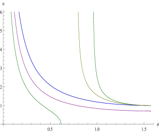
Figure 11: The real solution of the light-cone equation (106) for $A^{\mu}_{\parallel}$ as a function of $\theta$ when no external $B$ is present. We vary $\alpha=1/137\;(blue)$, $1\;(purple)$, $1.5\;(green)$, $2\;(yellow)$. The black ($\simeq$ blue) curve is $1/\sin\theta$.

It is conspicuous that one cannot trust the results when $\theta\to 0$ because they diverge. Furthermore, all curves below $\frac{1}{s_{\theta}}$ are to be rejected since we have shown that no such solution can exist. Last, one notes the presence of a pole at $s_{\theta}^{2}=\frac{1}{\alpha}$ for $\alpha>1$.

All these restrictions make the approximation of considering $n\in{\mathbb{R}}$ obviously very hazardous. This is why we shall perform in subsection 6.4 a detailed study with $n\in{\mathbb{C}}$.

6.4 Solutions for $\boldsymbol{A^{\mu}_{\parallel}}$ with $\boldsymbol{n\in{\mathbb{C}}}$

6.4.1 There is no solution with $\boldsymbol{n_{1}<\frac{1}{s_{\theta}}}$

When supposing $n\in{\mathbb{R}}$, we have seen that the solution with $n<\frac{1}{s_{\theta}}$ was unstable, in particular above $\theta_{max}$ such that $(\sin\theta_{max})^{2}=\frac{1}{\alpha}$ were it did not exist anymore.

Careful investigations for $n\in{\mathbb{C}}$ show that, like in the presence of $B$, no solution with $n_{1}<\frac{1}{s_{\theta}}$ exists .

6.4.2 The solution with $\boldsymbol{n_{1}>\frac{1}{s_{\theta}}}$

In the presence of an external $B$, we have seen that the solution with a quasi-real index suddenly disappears below an angle $\theta_{min}\approx\frac{1}{\Upsilon}$. In the present case with no external $B$, there is no $\theta_{min}$ but the index becomes “more and more complex” (that is the ratio of its imaginary and real parts increase) when $\theta$ becomes smaller and smaller.

To demonstrate this, we study the light-cone equation (106) for $A^{\mu}_{\parallel}$ with $n=n_{1}+in_{2},\ n_{1},n_{2}\in{\mathbb{R}}$. For practical reasons, we shall limit ourselves to the expansion of $V$ at small $\eta$ and $n_{2}$, valid when the two poles of $V$ lie in different 1/2 planes, given in (94).

The results are displayed in Figure 12 below, for $\alpha=1$ (blue), $\alpha=1.5$ (purple) and $\alpha=2$ (green). The values of $n_{1}$ are plotted on the left and the ones of $n_{2}$ on the right. The value of the other parameters are $u=.5,\eta=\frac{5}{1000}$. For $\alpha=\frac{1}{137}$, $n_{1}$ is indistinguishable from $\frac{1}{s_{\theta}}$.

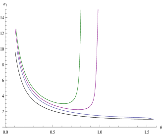
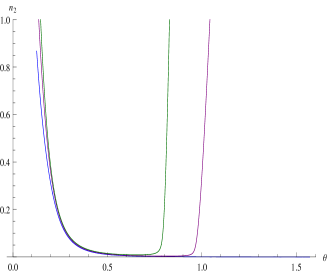
Figure 12: The real part $n_{1}$ (left) and imaginary part $n_{2}$ (right) of the solution $n$ of the light-cone equation (106) for $A^{\mu}_{\parallel}$ in the absence of external $B$. The blue curves correspond to $\alpha=1$, the purple curves to $\alpha=1.5$ and the green curves to $\alpha=2$. The black curve on the left is $n_{1}=\frac{1}{s_{\theta}}$.

$\bullet$ As $\theta$ gets smaller and smaller, the index becomes complex with larger and larger values of both its components. It is of course bounded as before to $|n|<\frac{1}{\eta}$ by quantum considerations. The brutal transition at $\theta_{min}\simeq\frac{1}{\Upsilon}$ is replaced by a smooth transition (which could be anticipated since, in the absence of $B$, the parameter $\Upsilon$ does not exist).

$\bullet$ A divergence occurs at large $\theta$ for $\alpha>1$, obviously reminiscent of the one that occurred in the approximation $n\in{\mathbb{R}}$ at $\theta=\theta_{max},(\sin\theta_{max})^{2}=\frac{1}{\alpha}$ for the solution $n<\frac{1}{s_{\theta}}$ (we had noticed that this condition could no longer be satisfied since, for $s^{2}_{\theta}>\frac{1}{\alpha}$, $n$ could only be larger than $\frac{1}{s_{\theta}}$).

Three explanations come to the mind concerning this singularity. The first is that, for large values of $n_{2}$, the expansion (94) that we used for $V$ is no longer valid; however, using the exact expression for the transmittance leads to the same conclusion. The second, and also very likely one, is that the perturbative series becomes very hazardous for $\alpha>1$ [25] (2-loop corrections become larger than 1-loop etc ); using a 2-loop calculation of the vacuum polarization without external $B$ seems feasible but also goes beyond the scope of this work. The third is that this divergence is the sign that some physical phenomenon occurs, like total reflexion, for $\theta>\theta_{max}$, which can only be settled by experiment. It is also known [24] that chiral symmetry breaking can occur for $\alpha>\alpha_{c}$.

$\bullet$ These calculations show in which domain the approximation $n\in{\mathbb{R}}$ is reliable since it requires $n_{2}\ll 1$: for example $n_{2}<.1$ needs $.3\leq\theta\leq\theta_{max}$, which leaves (except for $\alpha\leq 1$ in which case $\theta_{max}\geq\frac{\pi}{2}$) only a small domain for $\theta$.

$\bullet$ A very weak dependence on $\boldsymbol{\alpha}$ for $\boldsymbol{\theta<\theta_{max}}$

In the absence of external $B$ and away from the “wall” at large $\theta$, the index is seen to depend very little on $\alpha$. The dependence of $n$ on $\theta$ is practically only due to the transmittance function $V$ and to the confinement of electrons inside graphene. Notice in particular that, when $\alpha=\frac{1}{137}\ll 1$, the curve is indistinguishable from that of $\frac{1}{s_{\theta}}$.

The fairly large dependence on $\alpha$ that we uncovered in the presence of $B$ is therefore triggered by $B$ itself.

$\bullet$ The dependence on the energy of the photon

The dependence on $\eta$ only occurs in the imaginary part $n_{2}$ of $n$. This is shown in Figure 13, in which we vary $\eta$ in the visible spectrum, $\eta\in[\frac{2}{1000},\frac{7}{1000}]$ at $\alpha=1.5$ (unlike in Figure 12, $\theta$ has not been extended above $\theta_{max}$).

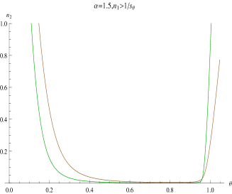
Figure 13: $n_{2}$ as a function of $\theta$ for $\eta=\frac{2}{1000}$ (green) and $\eta=\frac{7}{1000}$ (brown), in the case $\alpha=1.5$.

6.5 The limit of very small $\boldsymbol{\theta}$ ; absorption of visible light and experimental opacity

6.5.1 At small $\boldsymbol{\theta}$

Since absorption of visible light by graphene at close to normal incidence has been measured [15], let us show that our simple model gives predictions that are compatible with these measurements. To that purpose, we calculated numerically the index $n$ at the lowest value of $\theta$ at which the 2 poles of $V$ lie in different 1/2 planes. We did not make any expansion for $V$ (the price to pay is of course that no analytical expression is available) and obtained

$$\begin{split}\ast\ &for\ \alpha=1\ and\ \theta=\frac{\pi}{105.9}:n=41.20+.7\times i,\cr\ast\ &for\ \alpha=2\ and\ \theta=\frac{\pi}{89}:n=40+1\times i.\end{split}$$ (110)

The two corresponding angles are small enough to be considered close to normal incidence.

The real part of the index is seen to grow to large values, but it is not our concern here since the opacity is determined by $n_{2}$. The transmission coefficient along $z$ (therefore for $c_{\theta}\approx 1$) is given by

$$T=e^{-8\pi\eta n_{2}c_{\theta}}\approx 1-8\pi\eta n_{2},$$ (111)

while experimental measurements [15] are compatible with

$$T\approx 1-\pi\,\alpha_{vac},\ \alpha_{vac}=\frac{1}{137}.$$ (112)

This requires

$$n_{2}\approx\frac{\alpha_{vac}}{8\eta}\in[.57,.31]\ for\ \eta\in\left[\frac{1.6}{1000},\frac{2.9}{1000}\right],$$ (113)

in which the values of $\eta$ correspond to the ones evaluated for visible light in subsection 5.1.

We get therefore a reasonable order of magnitude for $n_{2}$. The factor $\sim 2$ of discrepancy between our prediction and the experimental value can be thought as an estimate of higher order corrections to the vacuum polarization.

6.5.2 At $\boldsymbol{\theta=0}$

Like at $B\not=0$ we come back to the light-cone equation (8). The transmittance $V$ has the same expression at small $\eta$ given in (72) and, using $T^{22}_{\xcancel{B}}=-T^{11}_{\xcancel{B}}=\pm i\frac{\pi\alpha}{2}q_{0}$ obtained from (105), one gets finally

$$q_{0}(1-n^{2})\left[(\beta_{1}^{2}+\beta_{2}^{2})q_{0}\pm i\frac{\alpha}{4}\eta^{2}p_{3}^{m}(\beta_{2}^{2}-\beta_{1}^{2})\right]=0$$ (114)

which has $n=1$ for only solution. So, like at $B\not=0$, the index goes to its trivial value at exactly normal incidence.

Like for $B\not=0$, we are at a loss to give a reliable description of the transition between $\theta$ small and $\theta=0$: our model and the approximations that we made certainly fail at some point since continuity looks very hard to achieve in this narrow domain.

6.6 Comparison with the case $\boldsymbol{B\not=0}$

Like in the presence of $B$, no non-trivial solution exists for the transverse polarization of the electromagnetic wave. Though the dimensional reduction that occurs in the presence of $B$ can no longer be invoked, this makes, in practice, the solution for $A^{\mu}_{\parallel}$ only depend on $\Pi^{11}$ and $\Pi^{33}$ (the latter being no longer equal to $-\Pi^{00}$).

When $B\not=0$, we suggested that the large modifications to the propagation of photons inside graphene are due to the magnetic resonance of the spins of electrons, by the combined action of the static $B$ and of the oscillating $b$ perpendicular to $B$. When $B=0$, no such enhancement is then expected to occur, which is confirmed by our results. They only display a weak dependence on $\alpha$.

Notice that, paradoxically, the case $B=0$ looks more tedious to handle. The behavior of the perturbative series at “fixed order” seems indeed to become rapidly uncontrollable when $\alpha$ grows. This phenomenon has already been noticed [25], and techniques going beyond standard perturbation theory (Random Phase Approximation, Dyson-Schwinger equations …) are then probably needed.

In subsection 7.3 we shall give other arguments why, in connexion with the massless Schwinger model, 1-loop calculations in the presence of a large external $B$ maybe more reliable.

7 Conclusion and prospects

We would like to summarize not only the salient properties and achievements of our description of graphene in external magnetic field, but also its odds and weirds, and its limitations.

7.1 Outlook

We have shown that, in the presence of a constant uniform external magnetic field, the refractive index of graphene is very sensitive to 1-loop quantum corrections. The effects, which only concern the “transverse magnetic” polarization of photons, are large for optical wavelengths and for magnetic fields even below 20 Tesla. They only depend (at least for the real part of the refractive index), on the ratio $c\frac{\sqrt{2\hbar eB}}{q_{0}}$. In particular, refractive effects grow like $\sqrt{eB}$ (as compared with a growth $\propto eB$ in the vacuum for supercritical magnetic fields demonstrated in [4]), but new quantum effects are expected at $B\geq B^{m}$ which will probably modify the behavior of $n$.

At the opposite, in the absence of external $B$, quantum effects stay small and the optical properties of graphene are mainly controlled by the transmittance function which incorporates the geometry of the sample and the confinement along $z$.

The behavior of $n$ as $\theta$ becomes small has been found to be different whether $B\not=0$ or $B=0$. When $B\not=0$ a brutal transition at $\theta_{min}\approx\frac{1}{\Upsilon}$ occurs below which the quasi-real solution valid above this threshold disappears, presumably (but this is still to be proved rigorously) in favor of a complex solution with large values of $n_{1}$ and $n_{2}$ (see subsection 7.2). At $B=0$ the transition is smooth: $n$ becomes gradually complex with larger and larger values of its real and imaginary components. Unfortunately, the domains of reliability of our calculations do not overlap such that the transition $B\to 0$ cannot be achieved smoothly from the case $B\not=0$ which is only reliable at $B$ “large”. Efforts are therefore needed to perform calculations valid in a wider range of $B$, which allows in particular a continuous transition to $B=0$.

Our description of graphene differs from what is usually done and it may be useful to summarize it. It has been considered, in position space, as $3+1$ dimensional, with a very small thickness $2a$. Electrons at the Dirac points have been described as massless Dirac-like particles with a vanishing “classical” momentum along $z$. An important feature of our calculation is confining the $\gamma\,e^{+}e^{-}$ vertices inside the very narrow graphene strip thanks to a calculation in position space of the photon propagator. This confinement in the direction of $B$ goes along with quantum fluctuations of the corresponding electronic momenta and for the momentum of the photon, which play important roles. This makes our approach depart not only from a description of electrons by a QFT in 2+1 dimensions, but also from a too restrictive brane-like model in which electrons live in 2+1 dimensions while gauge fields live in 3+1. In this respect, the sole calculation of the genuine vacuum polarization $\Pi_{\mu\nu}$, would it be in “reduced $QED_{4,3}$” [26], skips the transmittance $U$ and may not fully account for the optical properties of graphene. This looks specially true at $B=0$, where the index $n$ is mainly controlled by $U$. However, the situation could improve at very large $B$ because, as can be seen on Figure 5, for $\alpha\geq 1$ and inside the zone of confidence, $n$ only displays a weak dependence on $\theta$ and seems rather weakly constrained by the “leading” $\frac{1}{s_{\theta}}$ behavior coming from $U$. Since $U$, unlike $T^{\mu\nu}$, is independent of both $B$ and $\alpha$, their relative influence should decrease as they themselves increase: $n$ might then mostly depend on (seemingly resonant) effects controlled by $T^{\mu\nu}$.

We furthermore used $c$ and not $v_{F}$ inside the electron propagators because, at the idealized limit of a graphene strip with infinite horizontal extension $L\to\infty$ that we are considering, the Coulomb energy of an electron inside the medium is expected to vanish and the quantum fluctuations of their momentum along $B$ make them mostly propagate outside graphene. When $c$ is “decreased”, which corresponds to electrons more and more “confined into graphene”, we have found that the effects of $B$ on the refractive index increase.

Because of the approximations that we have made, and that we list below, we cannot pretend to have devised a fully realistic quantum model. We have indeed:
* truncated the perturbative series at 1-loop; there are hopes, however (see subsection 7.3) that, for a strong external $B$, this is a reasonable approximation;
* truncated the expansion of the electron propagator for large $B$ at next-to-leading order;
* approximated an incomplete $\beta$ function $F(x)=(-2)^{(-1+x)}\beta(-2,1-x,0)\approx\frac{1}{1-x}$, which in particular forget about poles at $p_{0}^{2}=2neB$ except for $n=1$; this is however safe for electrons with energy less than $13\sqrt{B(T)}\;(eV)$, which is always achieved when they are created from photons in the visible spectrum;
* chosen the Feynman gauge for the external photons;
* studied light-cone equations only through their expansions at large $\Upsilon=c\frac{\sqrt{2\hbar eB}}{q_{0}}$ and small $\eta=aq_{0}/\hbar c$. The small values of $\eta$ that occur in the visible spectrum guarantee that virtual created from photons have energies small enough to stay in the linear (Dirac) part of the spectrum.

In our favor, that we have gone beyond the limit $B\to\infty$ in the electron propagator is very fortunate because the effects induced on the refractive index are due to sub-leading terms.

We have worked in domains of wavelengths and magnetic fields in which our specific expansions and approximations are under control. Magnetic fields smaller or equal to $20\,T$ are fairly common practice today, and at $20\,T$ the degeneracy of the Landau level at the Dirac point is not yet lifted.
The large effects that we have obtained appear less surprising when they are realized to occur at suitable conditions for electron spin resonance.

Some additional remarks are due concerning the dimensionality of the problem (see also subsection 7.3). When $B\to\infty$, the Larmor radius of electrons vanishes like $\frac{1}{\sqrt{eB}}$ such that, the degrees of freedom orthogonal to $B$ shrinking to $0$, the physics becomes $1+1$ dimensional (see for example [11]). This is generally associated, in standard QED, with the projector $(1-i\gamma^{1}\gamma^{2})$ that controls, at this limit, the electron propagator. We have seen that, for graphene at large $B<\infty$, the situation is more subtle but dimensional reduction still arises through the integration over the electronic transverse degrees of freedom. The resulting two extra powers of $eB$ counter-balance the inverse powers occurring in the non-leading terms of the electron propagator, always dropped at $B=\infty$, and promote $\Pi^{00}$ and $\Pi^{33}$ as the two dominant components of the vacuum polarization. The transverse motion of electrons therefore plays for graphene an important role.

The direction “3” parallel to the external $B$ definitely also plays an essential role, not only by the prominence of $\Pi^{33}$ in the light-cone equation for $A^{\mu}_{\parallel}$, but also, by its “squeezing” to $2a$ and, through the confinement of the $\gamma\,e^{+}e^{-}$ vertices, by the large quantum fluctuations of the electron momentum that control the leading $1/s_{\theta}$ behavior of the refractive index.
The three directions of motion of the virtual electrons therefore collaborate to produce the effects on $n$ that we calculated.

A tantalizing question concerns of course the magnitude of higher order corrections. If 1-loop corrections to $n$ are large, how can we trust the result, unless all higher orders are proved to be much smaller? At present we have no answer to this. That $\alpha\simeq 2$ inside graphene is already a bad ingredient for a reliable perturbative treatment and, furthermore, the corrections to $n$ do not look like a standard series in powers of $\alpha$. Comparisons can be made for example with the results obtained in the case of non-confined massive electrons with the effective Euler-Heisenberg Lagrangian. The equations (2.17) (2.18) of [10] show quantum corrections to $n$ proportional to $\alpha\left(\frac{eB}{m_{e}^{2}}\right)^{2}$. In the study of the hydrogen atom [2][3], typical corrections are proportional to $\alpha\frac{eB}{m_{e}^{2}}$. In the present study, electrons are massless, and dimensionless factors are built with $q_{0}$ in place of $m_{e}$. Quantum corrections to the leading $\frac{1}{s_{\theta}}$ behavior of the index come out proportional to $\left(\frac{\alpha}{\pi}\right)^{2}\frac{eB}{q_{0}^{2}}$ (see (75)). While, at $B=0$ the situation looks very delicate to handle, the case of a large external $B$ looks more promising. We shall make a few remarks that motivate this optimism in subsection 7.3 in connection with the dimensional reduction $D\to D-2$ already evoked and with the massless Schwinger model.

A delicate and unresolved issue is the transition to $\theta=0$, at $B\not=0$ as well as at $B=0$. The only solution to the light-cone equation at $\theta=0$ is the trivial $n=1$ while at small $\theta\not=0$ the non-trivial solution that we exhibited behaves like $\frac{1}{s_{\theta}}$. Nature may choose everywhere the solution $n=1$, but, then, one should understand why the one on which we focused gets rejected. A possibility is also that the two solutions coexist down to $\theta=\theta_{\min}$, below which light can only propagate with $n=1$.

What happens to an external light beam intersecting a graphene strip is also unclear. That we stand very far from geometrical optics (see section 1), and that the Snell-Descartes laws of refraction for plane waves cannot be satisfied (we have indeed seen that $n\sin\theta>1$ inside graphene), are signals that the situation is not standard.

Last, hints exist that we only studied in this work most simple aspects of the optical behavior of graphene in an external magnetic field. We just make in subsection 7.2 below a few remarks concerning the possible existence of other solutions to the light-cone equations. This may however prove a Pandora box that we do not intend to open here.

7.2 Are there other solutions with a large absorption ?

We have seen that, as $\theta$ decreases, a transition occurs at $\theta\sim\frac{1}{\Upsilon}=\frac{q_{0}}{c\sqrt{2\hbar eB}}$: the quasi-real solution that we have exhibited for larger angles “disappears”.

If one considers, below the threshold, at the same $\theta=\frac{\pi}{17}$ the same Figure 9 drawn on a much larger domain for $n_{1}$ and $n_{2}$, one gets Figure 14. One solution (at least) occurs for the light-cone equation (97), which corresponds to $n_{1}\approx 6.5,n_{2}\approx 7$.

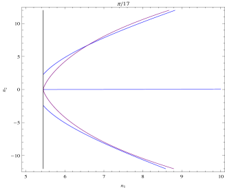
Figure 14: Solutions $(n_{1},n_{2})$ of the real part (purple) and imaginary part (blue) of the light-cone equation (97) for $A^{\mu}_{\parallel}$ at $\theta=\frac{\pi}{17}$ in the presence of $B$. The black vertical line on the left corresponds to $n_{1}=\frac{1}{s_{\theta}}$.

This suggests that below $\theta_{min}$, the system goes to a large index with a large absorption. This type of solution is incompatible with the approximations that we have made to find them $|n_{2}|\ll n_{1}$ etc, such that drawing a definitive conclusion requires using more elaborate numerical methods.

Such solutions with large index/absorption may exist even for $\theta>\theta_{min}$, that is jointly with the quasi-real solutions that we have focused on in this work.

7.3 Physics in strong external $\boldsymbol{B}$ and the Schwinger model

The electromagnetic coupling $\alpha$ being as large as $2.3$ in suspended graphene, the fate of any perturbative attempt looks a priori very gloomy, and the prospects are indeed dark in the absence of external $B$.

However, in presence of a large external $B$, the situation could be much better. If we forget about graphene, 4-dimensional “standard” Quantum Electrodynamics of massive electrons in strong external $B$ shares many properties with that of QED in 2 dimensions without $B$ (see for example [1][2] and references therein). The limit of massless fermions is specially attractive since the massless Schwinger model has remarkable characteristics: radiative corrections to the photon propagator stop at 1-loop (it is anomalous and keeps non-vanishing and constant while higher orders are both convergent and proportional to the (vanishing) electron mass), and the vacuum polarization tensor is not transverse (while preserving gauge invariance). The latter writes, up to 1-loop, $\Pi^{\mu\nu}(q)=(g^{\mu\nu}q^{2}-q^{\mu}q^{\nu})\left(1-\frac{e^{2}}{\pi\,q^{2}}\right)+q^{\mu}q^{\nu}$, and corresponds to a photon with mass $m_{\gamma}=\frac{e}{\sqrt{\pi}}$ [27].

When dealing with graphene, we are precisely, on the Dirac cones, concerned with massless electrons. Furthermore, as we have seen, the dimensional reduction $D\to D-2$ still operates .

However, the calculation that we have done differs from standard QED since, in particular, the log divergent integral typical of the massless Schwinger model has been split in $\mu=\int dp_{3}$ that factored out and was regularized with the cutoff $p_{3}^{m}$, $\times$ convergent integrals $B,C,D$ (53) over $p_{0}$. We have seen furthermore that the leading terms $\Pi^{33}=-\Pi^{00}$ of the vacuum polarization tensor are generated by non-leading contributions in the expansion at large $B$ of the electronic propagators.

This is why more detailed investigations are needed to establish whether a correspondence exists between graphene in strong external $B$ and the massless Schwinger model. Among the goals is of course providing reliable arguments that our 1-loop results stay reliable beyond this approximation, and that the non-transversality of the vacuum polarization tensor reveals the presence of a massive photon, which can then be expected to screen the Coulomb potential. This would provide a sensible access to electron-electron interactions inside graphene in the presence of an external $B$.

This will be the object of a subsequent work.

7.4 Other open issues

In the course of this study, we noticed several intriguing features: for $B\not=0$, the non-trivial solution of the light-cone equation seems to undergo a brutal transition at $\theta=\theta_{min}$, new quantum effects can be expected at $B>B^{m}$, and, even at $B=0$, something dramatic happens at $\alpha\geq 1$ since $n$ diverges for $\theta\geq\theta_{max}$ such that $\sin^{2}_{\theta_{max}}=\frac{1}{\alpha}$. These can be only artifacts of the approximations that we made, adding to the poor reliability of a fixed order perturbative expansion for a strongly coupled system; but some could also be signals of phenomena like total reflection of light, chiral symmetry breaking, spontaneous pair production, screening of the Coulomb interaction (massive photon) …, or of yet unsuspected phenomena or phase transitions. Graphene could then also prove a privileged test-ground for the interplay between Quantum Field Theory, quantum optics and nanophysics. Experimental testing and guidance is of course strongly wished for.

Acknowledgments: it is a pleasure to thank M. Vysotsky for his continuous interest and encouragements. We are also very indebted to B. Douçot and J.N. Fuchs for their comments and advice. Erroneous statements are of course our sole responsibility.

Appendix A Demonstration of eq. (17)

We start from (14), in which, now, the fermion propagator $G$ depends on $B$. The notations are always $v=(v_{0},v_{1},v_{2},v_{3})=(\hat{v},v_{3}),\hat{v}=(v_{0},v_{1},v_{2})$.

$$\begin{split}\Delta^{\rho\sigma}(x,y)&=e^{2}\int d^{3}\hat{u}\int_{-a}^{+a}du_{3}\int d^{3}\hat{v}\int_{-a}^{+a}dv_{3}\cr&\int\frac{d^{4}q}{(2\pi)^{4}}\;e^{iq(u-x)}\Delta^{\rho\mu}(q)\,\gamma_{\mu}\int\frac{d^{4}p}{(2\pi)^{4}}\;e^{ip(u-v)}G(\hat{p},B)\,\gamma_{\nu}\int\frac{d^{4}r}{(2\pi)^{4}}\;e^{ir(v-u)}G(\hat{r},B)\int\frac{d^{4}s}{(2\pi)^{4}}\;e^{is(y-v)}\Delta^{\sigma\nu}(s)\cr&=e^{2}\int d^{3}\hat{u}\int_{-a}^{+a}du_{3}\int d^{3}\hat{v}\int_{-a}^{+a}dv_{3}\;\int\frac{d^{3}q}{(2\pi)^{3}}\frac{dq_{3}}{2\pi}\;e^{i\hat{q}(\hat{u}-\hat{x})}e^{iq_{3}(u_{3}-x_{3})}\Delta^{\rho\mu}(q)\cr&\hskip 42.67912pt\gamma_{\mu}\int\frac{d^{3}\hat{p}}{(2\pi)^{3}}\,\frac{dp_{3}}{2\pi}\;e^{i\hat{p}(\hat{u}-\hat{v})}e^{ip_{3}(u_{3}-v_{3})}G(\hat{p},B)\,\gamma_{\nu}\int\frac{d^{3}\hat{r}}{(2\pi)^{3}}\,\frac{dr_{3}}{2\pi}\;e^{i\hat{r}(\hat{v}-\hat{u})}e^{ir_{3}(v_{3}-u_{3})}G(\hat{r},B)\cr&\hskip 42.67912pt\int\frac{d^{3}\hat{s}}{(2\pi)^{3}}\,\frac{ds_{3}}{2\pi}\;e^{i\hat{s}(\hat{y}-\hat{v})}e^{is_{3}(y_{3}-v_{3})}\Delta^{\sigma\nu}(s)\cr&=e^{2}\underbrace{\int d^{3}\hat{u}\;e^{i\hat{u}(\hat{q}+\hat{p}-\hat{r})}}_{(2\pi)^{3}\delta(\hat{p}+\hat{q}-\hat{r})}\int d^{3}\hat{v}\;e^{i\hat{v}(-\hat{p}+\hat{r}-\hat{s})}\int_{-a}^{+a}du_{3}\int_{-a}^{+a}dv_{3}\;\int\frac{d^{3}\hat{q}}{(2\pi)^{3}}\,\frac{dq_{3}}{2\pi}\;e^{i\hat{q}(-\hat{x})}e^{iq_{3}(u_{3}-x_{3})}\Delta^{\rho\mu}(q)\cr&\hskip 42.67912pt\gamma_{\mu}\int\frac{d^{3}\hat{p}}{(2\pi)^{3}}\,\frac{dp_{3}}{2\pi}\;e^{ip_{3}(u_{3}-v_{3})}G(\hat{p},B)\,\gamma_{\nu}\int\frac{d^{3}\hat{r}}{(2\pi)^{3}}\,\frac{dr_{3}}{2\pi}\;e^{ir_{3}(v_{3}-u_{3})}G(\hat{r},B)\cr&\hskip 42.67912pt\int\frac{d^{3}\hat{s}}{(2\pi)^{3}}\,\frac{ds_{3}}{2\pi}\;e^{i\hat{s}(\hat{y})}e^{is_{3}(y_{3}-v_{3})}\Delta^{\sigma\nu}(s)\cr&=e^{2}\underbrace{\int d^{3}\hat{v}\;e^{i\hat{v}(\hat{q}-\hat{s})}}_{(2\pi)^{3}\delta(\hat{q}-\hat{s})}\int_{-a}^{+a}du_{3}\int_{-a}^{+a}dv_{3}\;\int\frac{d^{3}\hat{q}}{(2\pi)^{3}}\,\frac{dq_{3}}{2\pi}\;e^{i\hat{q}(-\hat{x})}e^{iq_{3}(u_{3}-x_{3})}\Delta^{\rho\mu}(q)\cr&\hskip 42.67912pt\gamma_{\mu}\int\frac{d^{3}\hat{p}}{(2\pi)^{3}}\,\frac{dp_{3}}{2\pi}\;e^{ip_{3}(u_{3}-v_{3})}G(\hat{p},B)\,\gamma_{\nu}\int\frac{dr_{3}}{2\pi}\;e^{ir_{3}(v_{3}-u_{3})}G(\hat{p}+\hat{q},B)\cr&\hskip 42.67912pt\int\frac{d^{3}\hat{s}}{(2\pi)^{3}}\,\frac{ds_{3}}{2\pi}\;e^{i\hat{s}(\hat{y})}e^{is_{3}(y_{3}-v_{3})}\Delta^{\sigma\nu}(s)\cr&=e^{2}\int_{-a}^{+a}du_{3}\int_{-a}^{+a}dv_{3}\;\int\frac{d^{3}\hat{q}}{(2\pi)^{3}}\,\frac{dq_{3}}{2\pi}\;e^{i\hat{q}(-\hat{x})}e^{iq_{3}(u_{3}-x_{3})}\Delta^{\rho\mu}(\hat{q},q_{3})\cr&\hskip 42.67912pt\gamma_{\mu}\int\frac{d^{3}\hat{p}}{(2\pi)^{3}}\,\frac{dp_{3}}{2\pi}\;e^{ip_{3}(u_{3}-v_{3})}G(\hat{p},B)\,\gamma_{\nu}\int\frac{dr_{3}}{2\pi}\;e^{ir_{3}(v_{3}-u_{3})}G(\hat{p}+\hat{q},B)\int\frac{ds_{3}}{2\pi}\;e^{i\hat{q}(\hat{y})}e^{is_{3}(y_{3}-v_{3})}\Delta^{\sigma\nu}(\hat{q},s_{3})\cr&=e^{2}\int\frac{dr_{3}}{2\pi}\int\frac{ds_{3}}{2\pi}\int_{-a}^{+a}du_{3}\;e^{iu_{3}(q_{3}+p_{3}-r_{3})}\int_{-a}^{+a}dv_{3}\;e^{iv_{3}(-p_{3}+r_{3}-s_{3})}\cr&\hskip 28.45274pt\int\frac{d^{3}\hat{q}}{(2\pi)^{3}}\,\frac{dq_{3}}{2\pi}\;e^{i\hat{q}(-\hat{x})}e^{iq_{3}(-x_{3})}\Delta^{\rho\mu}(\hat{q},q_{3})\,\gamma_{\mu}\int\frac{d^{3}\hat{p}}{(2\pi)^{3}}\,\frac{dp_{3}}{2\pi}\;G(\hat{p},B)\,\gamma_{\nu}\,G(\hat{p}+\hat{q},B)e^{i\hat{q}(\hat{y})}e^{is_{3}(y_{3})}\Delta^{\sigma\nu}(\hat{q},s_{3})\cr&=\int\frac{dp_{3}}{2\pi}\int\frac{dq_{3}}{2\pi}\int\frac{dr_{3}}{2\pi}\int\frac{ds_{3}}{2\pi}\int_{-a}^{+a}du_{3}\;e^{iu_{3}(q_{3}+p_{3}-r_{3})}\int_{-a}^{+a}dv_{3}\;e^{iv_{3}(-p_{3}+r_{3}-s_{3})}\cr&\hskip 42.67912pt\int\frac{d^{3}\hat{q}}{(2\pi)^{3}}\;e^{i\hat{q}(\hat{y}-\hat{x})}e^{iq_{3}(-x_{3})}e^{is_{3}(y_{3})}\Delta^{\rho\mu}(\hat{q},q_{3})\Delta^{\sigma\nu}(\hat{q},s_{3})\ \underbrace{e^{2}\int\frac{d^{3}\hat{p}}{(2\pi)^{3}}\;\gamma_{\mu}\,G(\hat{p},B)\,\gamma_{\nu}\,G(\hat{p}+\hat{q},B)}_{iT_{\mu\nu}(\hat{q},B)},\end{split}$$ (115)

which is eq. (17).

Appendix B Approximate Coulomb energy of a graphene electron

Let us consider, to simplify, a circular graphene strip of radius $L$. We need to evaluate the Coulomb energy of an electron inside graphene, due to the rest of the medium with global charge $+1$. We consider that it is uniformly spread such that the charge density per unit surface is $\frac{e}{\pi L^{2}}$ and, inside the two circles of radii $r$ and $r+dr$ lies a charge $\frac{e}{\pi L^{2}}2\pi rdr$. It contributes to the Coulomb energy of the electron by $-\frac{e}{r}\frac{e}{\pi L^{2}}2\pi rdr=-\frac{2e^{2}}{L^{2}}dr$. The total electrostatic energy of this electron is accordingly $-\int_{0}^{L}dr\;\frac{2e^{2}}{L^{2}}=-\frac{2e^{2}}{L}$, which vanishes when $L\to\infty$.

The value given by the naive formula $-\frac{e^{2}}{4\pi\epsilon_{0}\,a}$ is $\simeq 8.2\,eV$. It corresponds to a charge $+1$ localized at distance $a$ from the electron.

The ionization energy of an electron inside graphene is given in [28], at the limit when the number of carbon atoms goes to infinity, by $E_{t}\simeq.1\frac{2\pi\hbar v_{F}}{3\,a_{c}\sqrt{3/4}}\approx 1.13\,eV$, in which $a_{c}=1.4\,10^{-10}\,m$ is the interatomic spacing. This value is smaller than all photon energies that we are considering (see subsection 5.1).

References

- [1] M.I. VYSOTSKY: “Atomic Levels in Superstrong Magnetic Fields and QED of Massive Electrons : Screening”, Pis’ma v ZhETF, 92 (2010) 22-26 (JETP Lett. 92 (2010) 15-20).
- [2] B. MACHET & M.I. VYSOTSKY: “Modification of Coulomb law and energy levels of the hydrogen atoms in a superstrong magnetic field”, Phys. Rev. D 83, 025022 (2011).
- [3] S.I. GODUNOV, B. MACHET & M.I. VYSOTSKY: “Critical nucleus charge in a superstrong magnetic field: Effects of screening”, Phys. Rev. D 85, 044058 (2012).
- [4] A.E. SHABAD: “Photon Propagation in a Supercritical Magnetic Field”, Zh. Eks. Teor. Fiz. 125 (2004) 210 (JETP 98 (2004) 186).
- [5] M.O. GOERBIG: “Electronic properties of graphene in a strong magnetic field”, Rev. Mod. Phys. 83 (2011) 1193, and references therein.
- [6] A.H. CASTRO NETO, F. GUINEA, N.M.R. PEREZ, K.S. NOVOSELOV & A.K. GEIM: “The electronic properties of graphene”, Rev. Mod. Phys. 81 (2009) 109.
- [7] J. SCHWINGER: “On Gauge Invariance and Vacuum Polarization”, Phys. Rev. 82, 664 (1951).
- [8] W. DITTRICH & M. REUTER: “Effective Lagrangian in Quantum Electrodynamics”, Lecture Notes in Physics 220 (Springer-Verlag, Berlin Heidelberg 1985).
- [9] WU-YANG TSAI & T. ERBER: “ Photon pair creation in intense magnetic fields”, Phys. Rev. D 10, 492 (1974).
- [10] W. DITTRICH & H. GIES: “Vacuum Birefringence in Strong Magnetic Fields”, hep-ph/9806417, Sandansky 1998, Frontier tests of QED and physics of the vacuum, 29-43.
- [11] A.E. SHABAD & V.V. USOV: “Electric field of a pointlike charge in a strong magnetic field and ground state of a hydrogenlike atom”, Phys. Rev. D 77, 025001 (2008).
- [12] N.M.R. PEREZ, A.H. CASTRO NETO & F. GUINEA : “ Dirac fermion confinement in graphene”, Phys. Rev. B 73, 241403(R) (2006).
- [13] S. GODUNOV: “Two-Loop Corrections to the Potential of a Pointlike Charge in a Superstrong Magnetic Field”, Yad. Fiz. 76 (2013) 955 [Phys. Atom. Nucl. 76 (2013) 901].
- [14] Y. ZHANG, Z. JIANG, J.P. SMALL, M.S. PUREWAL, Y.-W. TAN, M. FAZLOLLAHI, J.D. CHUDOW, J.A. JASZCZAK, H.L. STORMER & P. KIM: “Landau-Level Splitting in Graphene in High Magnetic Fields”, Phys. Rev. Lett. 96, 136806 (2006).
- [15] R.R. NAIR, P. BLAKE, A.N. GRIGORENKO, K.S. NOVOSELOV, T.J. BOOT, T. STAUBER, N.M.R. PEREZ & A.K. GEIM: “Fine Structure Constant Defines Visual Transparency of Graphene”, Science, vol. 320 (2008) 1308, and references therein.
- [16] V.P. GUSYNIN, V.A. MIRANSKY & I.A. SHOVKOVY: “Theory of the magnetic catalysis of chiral symmetry breaking in QED”, Nucl. Phys. B 563 (1999) 361-389.
- [17] WU-YANG TSAI: “Vacuum polarization in homogeneous magnetic fields”, Phys. Rev. D 10, 2699 (1974).
- [18] G. MODANESE: “General estimate of the graviton lifetime”, hep-th/9501123, Phys. Lett. B 348 (1995) 51-54.
- [19] M.E. PESKIN & D.V. SCHROEDER: “An Introduction to Quantum Field Theory”, Perseus Books (Reading, Massachusetts) 1995.
- [20] Y.W. SOKHOTSKI: “On definite integrals and functions used in series expansions” St. Petersburg, 1873. J. PLEMELJ: “Problems in the sense of Riemann and Klein”, Interscience Publishers, New York, 1964.
- [21] G.W. SEMENOFF: “Condensed-Matter Simulation of a Three-Dimensional Anomaly”, Phys. Rev. Lett. 53 (1984) 2449.
- [22] I.A. SHOVKOVY: “Magnetic Catalysis: A Review”, arXiv:1207.5081 [hep-ph], Lect. Notes Phys. 871 (2013) 13-49.
- [23] E.V. GORBAR, V.P. GUSYNIN, V.A. MIRANSKY & I.A. SHOVKOVY: “Magnetic driven metal-insulator phase transition in planar systems”, Phys. Rev. B 66, 045108 (2002).
- [24] O.V. GAMAYUN, E.V. GORBAR & V.P. GUSYNIN: “Supercritical Coulomb center and excitonic instability in graphene”, Phys. Rev. B 80, 165429 (2009).
- [25] E. BARNES, E.H. HWANG, R.E. THROCKMORTON & S. DAS SARMA: “Effective field theory, three-loop perturbative expansion, and their experimental implications in graphene many-body effects”, arXiv:1401.7011 [cond-mat.mes-hall], Phys. Rev. B 89, 235431 (2014). J. HOFMANN, E. BARNES & S. DAS SARMA: “Why does graphene behaves as a weakly coupled system ?”, arXiv:1405.7036 [cond-mat.mes-hall].
- [26] A.V. KOTIKOV & S. TEBER: “Two-loop fermion self-energy in reduced quantum electrodynamics and application to the ultra-relativistic limit of graphene”, arXiv:1312.2430 [hep-ph], Phys. Rev. D 89, 065038 (2014).
-
[27]
J. SCHWINGER: ”Gauge invariance and mass II”, Phys. Rev. 128 (1962) 2425;
see also:
J. ZINN-JUSTIN: “ Quantum Field Theory and Critical Phenomena”, International Series of Monographs on Physics - 77 (Clarendon Press, Oxford 1989), appendix A31-2 “The Schwinger Model”. - [28] M. GHADIRY, A. BIN ABD MANAF, M. NADI, M. RAHMANI & M.T. AHMADI: “Ionization coefficient of monolayer graphene nanoribbon”, Microelectronics Reliability 52 (2012) 1396-1400.