Observational constraints on Modified Chaplygin Gas from Large Scale Structure

Abstract

We study cosmological models with modified Chaplygin gas (in short, MCG) to determine observational constraints on its EoS parameters. The observational data of the background and the growth tests are employed. The background test data namely, $H(z)-z$ data, CMB shift parameter, Baryonic acoustic oscillations (BAO) peak parameter, SN Ia data are considered to study the dynamical aspects of the universe. The growth test data we employ here consists of the linear growth function for the large scale structures of the universe, models are explored assuming MCG as a candidate for dark energy. Considering the observational growth data for a given range of redshift from the Wiggle-Z measurements and rms mass fluctuations from Ly-$\alpha$ measurements, cosmological models are analyzed numerically to determine constraints on the MCG parameters. In this case, the Wang-Steinhardt ansatz for the growth index $\gamma$ and growth function $f$ (defined as $f=\Omega_{m}^{\gamma}(a)$) are also taken into account for the numerical analysis. The best-fit values of the equation of state parameters obtained here are used to study the variation of the growth function ($f$), growth index ($\gamma$), equation of state parameter ($\omega$), squared sound speed $c^{2}_{s}$ and deceleration parameter with redshift $z$. The observational constraints on the MCG parameters obtained here are then compared with those of the GCG model for viable cosmology. It is noted that MCG models satisfactorily accommodate an accelerating phase followed by a matter dominated phase of the universe. The permitted range of values of the EoS parameters and the associated parameters ($f$, $\gamma$, $\omega$, $\Omega$, $c^{2}_{s}$, $q$) are compared with those obtained earlier using other observations.

1 Introduction

Recent cosmological observations from supernova [1, 2, 3, 4, 5], WMAP [6, 7, 8, 9, 10], BAO data [11] predicted that the present universe is passing through a phase of accelerating expansion which might be fuelled due to the existence of a new source of energy which is termed as dark energy. In observational cosmology, the expansion rate $H(z)$ is measured at various redshifts which are useful to obtain different cosmological parameters namely, distance modulus parameter, deceleration parameter. Although the analysis provides us with a satisfactory understanding of cosmological dynamics, it fails to give a complete understanding of the evolution of the universe. Consequently, additional observational input, namely, cosmic growth of the inhomogeneous parts of the universe for its structure formation, is considered in recent times for observational analysis. The growth of the large scale structures derived from the linear matter density contrast $\delta(z)\equiv\frac{\delta\rho_{m}}{\rho_{m}}$ of the universe is considered as an important tool in constraining cosmological model parameters. In order to describe the evolution of the inhomogeneous energy density, it is preferable to parametrize the growth function $f=\frac{d\log\delta}{d\log a}$ in terms of the growth index $\gamma$. It was Peebles [12] who first initiated, and thereafter Wang and Steinhardt [13] parametrized $\delta$ in terms of $\gamma$ to obtain cosmologies which are useful in various contexts reported in the literature [14, 15, 16, 17, 18, 19, 20, 21, 22, 23]. The study of dark energy for understanding accelerating universe in cosmology is thus important which may be analyzed using observational data from the observed expansion rate $H(z)$ and growth of matter density contrast $\delta(z)$ data simultaneously.
It is known that in the general theory of relativity, ordinary matter fields available from the standard model of particle physics fails to account for the present observations of the universe. It is therefore essential to consider a new type of matter in the modified sector of matter in the Einstein-Hilbert action or a new physics in this connction. In the literature, Chaplygin gas (CG) was considered to be one such candidate for dark energy. The equation of state (henceforth, EoS) for CG is

$$p=-\frac{A}{\rho}$$ (1.1)

where $A$ is a positive constant. It may be important to mention here that the initial idea of a CG originated in aerodynamics [24]. CG may be considered as an alternative to quintessence [25]. In the context of string theory, CG emerges from the dynamics of a generalized d-brane in a (d+1,1) space time. It can be described by a complex scalar field which is obtained from a generalized Born-Infeld action. But CG is ruled out in cosmology as cosmological models are not consistent with observational data namely, SNIa, BAO, CMB etc. [26, 27]. Subsequently the equation of state for CG is generalized to incorporate different aspects of the observational universe. The equation of state for generalized Chaplygin gas (in short, GCG) [28, 29] is given by

$$p=-\frac{A}{\rho^{\alpha}}$$ (1.2)

with $0\leq\alpha\leq 1$. In the above EoS for $\alpha=1$ reduces to Chaplygin gas[24]. It has two free parameters $A$ and $\alpha$. It is known that GCG is capable of explaining the background dynamics [30] and various other features of a homogeneous isotropic universe satisfactorily. The features that the GCG corresponds to almost dust ($p=0$) at high density does not agree completely with our universe. It is also known that the model suffers from a serious problem at the perturbative level. The matter power spectrum of GCG exhibits strong oscillations or instabilities, unless GCG model reduces to $\Lambda$CDM [31]. The oscillations for the baryonic component with GCG leads to undesirable features in CMB spectrum [32].
In order to use the gas equation in a more satisfactory way, a modification to the GCG is further considered by adding a positive term, linear in density, to the EoS which is known as modified Chaplygin gas (in short MCG). The equation of state for the MCG is given by:

$$p=B\rho-\frac{A}{\rho^{\alpha}}$$ (1.3)

where $A$, $B$, $\alpha$ are positive constants with $0\leq\alpha\leq 1$. The above EoS reduces to that of GCG model [28, 29] when one sets $B=0$. A cosmological constant $\Lambda$ emerges by setting $\alpha=-1$ and $A=1+B$. For $A=0$, eq. (1.3) reduces to an EoS which describes a perfect fluid with $\omega=B$, e.g., a quintessence model [33]. The MCG contains one more free parameter, namely, $B$, over the GCG. It may be pointed out here that the MCG is a single fluid model which unifies dark matter and dark energy. The MCG model is suitable for obtaining constant negative pressure at low density accommodating late acceleration, and a radiation dominated era (with $B=\frac{1}{3}$) at high density. Thus a universe with a MCG may be described starting from the radiation epoch to the epoch dominated by the dark energy consistently. On the other hand the GCG describes the evolution of the universe from matter dominated to a dark energy dominated regime (as $B=0$). So compared to GCG, the proposed MCG is suitable to describe the evolution of the universe over a wide range of epoch [34]. On the otherhand the distinction between $\Lambda CDM$ and GCG models are very little, GCG is not very much suitable to describe EoS for the dark energy. Another motivation for considering MCG as a dark energy candidate is that the exact form of the EoS for dark energy is not yet known. The MCG is an attempt to find something interesting that is not exactly $\Lambda$CDM. Wu et al.[35] studied the dynamics of the MCG model. Bedran et al. [36] studied the evolution of the temperature function in the presence of a MCG. It is also consistent with perturbative study [37] and the spherical collapse problem [38]. In this paper we consider a universe with MCG for cosmological analysis.

In this paper observational constraints on EoS parameters of the MCG are determined using different observational data namely, H(z)-z data, the CMB shift parameter, BAO peak parameter, the SNIa data, the growth function and growth index in a FRW universe. The growth data given in Table -2 consists of a number of data points within redshift ranges (0.15 to 3.0) which is related to the growth function $f$. It may be pointed out here that the observed growth rate corresponds to various projects/surveys, including the latest Wiggle-Z measurements shown in the table. Gupta et al. [39] obtained constraints on GCG parameters using the above data. Cosmological models dominated by viscous dark fluids are also considered in Ref.[40] where it is shown that viscous fluid mimics a $\Lambda$CDM model when the coefficient of viscosity varies as $\rho^{-1/2}$. It also provides excellent agreement with both the supernova and ($H-z$) data. The viscous cosmological model is analogous to the GCG model. In addition to the above data, other observational sets of growth data given in (Table- 3) from various sources such as: the redshift distortion of galaxy power spectra [41], root mean square ($\it rms$) mass fluctuation $\sigma_{8}(z)$ obtained from galaxy and $\it Ly$-$\alpha$ surveys at various redshifts [42, 43], weak lensing statistics [44], baryon acoustic oscillations [11], X-ray luminous galaxy clusters [45], Integrated Sachs-Wolfs (ISW) Effect [46, 47, 48, 49, 50] etc. are important, and which will be taken up here. It is known that redshift distortions are caused by velocity flow induced by gravitational potential gradients which evolved due to the growth of the universe under gravitational attraction and dilution of the potentials due to the cosmic expansion. The gravitational growth index $\gamma$ is considered to be an important parameter which affects the redshift distortion [14]. The cluster abundance evolution, however, strongly depends on $\it rms$ mass fluctuations $\sigma_{8}(z)$ [13] which will be also considered here.

We adopt here $\it chi$-square minimization techniques to constrain different parameters of the EoS for a viable cosmological model considering a MCG as the fluid in the universe. In the analysis total $\it chi$-square is constituted with the background tests ((i) H(z)-z data (ii)The CMB shift parameter (iii) Baryonic acoustic oscillations (BAO) peak parameter (iv) The SN Ia data) and the growth tests. The best-fit values of the model parameters are then determined from the $\it chi$-square function to study the evolution of the universe.

The paper is organized as follows : In sec.2, relevant field equations obtained from the Einstein field equation are given. In sec.3, we determine constraints on the EoS parameters from background test. In sec.4, numerical analysis of the growth index parametrization in terms of the EoS parameters is given defining respective $\it chi$-square functions. In sec.5, constraints on the EoS parameters obtained from the background test and growth test are presented. In sec.6, a summary of the numerical analysis is presented. Finally, in sec.7, we give a brief discussion.

2 Einstein Field Equations

The Einstein field equation is given by

$$R_{\mu\nu}-\frac{1}{2}g_{\mu\nu}R=8\pi G\;T_{\mu\nu}$$ (2.1)

where $R_{\mu\nu}$, $R$, $g_{\mu\nu}$ and $T_{\mu\nu}$ represent the Ricci tensor, the Ricci scalar, the metric tensor in 4-dimensions and the energy momentum tensor respectively. We consider a Robertson-Walker metric which is given by

$$ds^{2}=-dt^{2}+a^{2}(t)\left[\frac{dr^{2}}{1-kr^{2}}+r^{2}(d\theta^{2}+sin^{2}\theta\;d\phi^{2})\right]$$ (2.2)

where $k=0,+1,-1$ represents flat, closed and open universe, and $a(t)$ is the scale factor of the universe with $r,\theta,\phi$ co-moving co-ordinates.

Using metric (2.2) in the Einstein field eq. (2.1), we obtain the following equations:

$$3\left(\frac{\dot{a}^{2}}{a^{2}}+\frac{k}{a^{2}}\right)=8\pi G\;\rho,$$ (2.3)

$$2\frac{\ddot{a}}{a}+\frac{\dot{a}^{2}}{a^{2}}+\frac{k}{a^{2}}=-8\pi G\;p,$$ (2.4)

where $\rho$ and $p$ represent the energy density and pressure respectively. The conservation equation is given by

$$\frac{d\rho}{dt}+3H\left(\rho+p\right)=0,$$ (2.5)

where $H=\frac{\dot{a}}{a}$ is Hubble parameter.

Using the EoS given by eq.(1.3) in eq.(2.5)and integrating once, one obtains the energy density for a modified Chaplygin gas which is given by

$$\rho_{mcg}=\rho_{0}\left[A_{s}+\frac{1-A_{s}}{a^{3(1+B)(1+\alpha)}}\right]^{\frac{1}{1+\alpha}}$$ (2.6)

where $A_{s}=\frac{A}{1+B}\frac{1}{\rho_{0}^{\alpha+1}}$ with $B\neq-1$, $\rho_{o}$ is an integration constant. The scale factor of the universe is related to the redshift parameter $z$ as $\frac{a}{a_{0}}=\frac{1}{1+z}$, one may choose the present scale factor of the universe $a_{0}=1$ for convenience. The MCG model parameters are $A_{s}$, $B$ and $\alpha$. From eq. (2.6), it is evident that the positivity condition for the energy density is ensured when $0\leq A_{s}\leq 1$. From eq. (2.6), one recovers the standard $\Lambda$CDM model for $\alpha=0$ and $B=0$. The Hubble parameter can be expressed as a function of redshift using the field eq. (2.3), which is given by

$$H(z)=H_{0}[\Omega_{b0}(1+z)^{3}+$$

$$\;\;\;(1-\Omega_{b0})[(A_{s}+(1-A_{s})(1+z)^{3(1+B)(1+\alpha)})^{\frac{1}{1+\alpha}}]]^{\frac{1}{2}}.$$ (2.7)

where $\Omega_{b0}$, $H_{0}$ represent the present baryon density and present Hubble parameter, respectively.

The square of the sound speed is given by

$$c^{2}_{s}=\frac{\delta p}{\delta\rho}=\frac{\dot{p}}{\dot{\rho}}$$ (2.8)

which reduces to

$$c^{2}_{s}=B+\frac{A_{s}\alpha(1+B)}{\left[A_{s}+(1-A_{s})(1+z)^{3(1+B)(1+\alpha)})\right]}.$$ (2.9)

In terms of the equation of state it becomes

$$c^{2}_{s}=-\alpha\omega+B(1+\alpha).$$ (2.10)

It may be mentioned here that for causality and stability under perturbations, it is necessary to satisfy the inequality condition $c_{s}^{2}\leq 1$ [33]. The deceleration parameter is given by

$$q(a)=\frac{\frac{\Omega_{b0}}{a^{3}}+\Omega_{mcg}(a)[1+3\omega(a)]}{2[\frac{\Omega_{b0}}{a^{3}}+\Omega_{mcg}(a)]}$$ (2.11)

where

$$\Omega_{mcg}(a)=\Omega_{mcg0}[A_{s}+\frac{(1-A_{s})}{a^{3(B+1)(1+\alpha)}}]^{\frac{1}{1+\alpha}}$$ (2.12)

3 Background tests from Observed Data

We consider the following background tests from observed cosmological data for analyzing cosmological models:
$\bullet$ The differential age of old galaxies, given by $H(z)$.
$\bullet$ The peak position of the Baryonic Acoustic Oscillations (BAO).
$\bullet$ The CMB shift parameter.
$\bullet$ The SN Ia data.

The EoS for the MCG contains three unknown parameters namely $A_{s}$, $B$ and $\alpha$, which are determined here by a numerical analysis employing different observed data. For the analysis, the Einstein field equation is rewritten in terms of the Hubble parameter, and a $\it chi$-square function is also defined corresponding to the observation under consideration.

3.1 $\chi^{2}$-function for Observed Hubble Data (OHD)

The observed Hubble Data is given in table (1) [51] are employed here: We define first the $\it chi$-square ($\chi^{2}_{H-z}$) function which is

$$\chi^{2}_{H-z}(H_{0},A_{s},B,\alpha,z)=\sum\frac{(H(H_{0},A_{s},B,\alpha,z)-H_{obs}(z))^{2}}{\sigma^{2}_{z}}$$ (3.1)

where $H_{obs}(z)$ is the observed Hubble parameter at red shift $z$ and $\sigma_{z}$ corresponds to the error associated with that particular observation as shown in table -1.

z	$H(z)$	$\sigma$
0.00	73	$\pm$ 8.0
0.10	69	$\pm$ 12.0
0.17	83	$\pm$ 8.0
0.27	77	$\pm$ 14.0
0.40	95	$\pm$ 17.4
0.48	90	$\pm$ 60.0
0.88	97	$\pm$ 40.4
0.90	117	$\pm$ 23.0
1.30	168	$\pm$ 17.4
1.43	177	$\pm$ 18.2
1.53	140	$\pm$ 14.0
1.75	202	$\pm$ 40.4

Table 1: $H(z)vs.z$ data from Stern et al. [51]

3.2 $\chi^{2}$-function for Baryon Acoustic Oscillation (BAO)

A model independent BAO peak parameter for low red shift $z_{1}$ measurements in a flat universe is given by [11]:

$$\mathcal{A}=\frac{\sqrt{\Omega_{m}}}{E(z_{1})^{1/3}}\left(\frac{\int^{z_{1}}_{0}\frac{dz}{E(z)}}{z_{1}}\right)^{2/3}$$ (3.2)

where $\Omega_{m}$ is the matter density parameter for the Universe. The $\it chi$-square function in this case is defined as :

$$\chi^{2}_{BAO}(A_{s},B,\alpha,z)=\frac{\left(\mathcal{A}-0.469\right)^{2}}{\left(0.017\right)^{2}}.$$ (3.3)

The Sloan Digital Sky Survey (SDSS) data for the Luminous Red Galaxies (LRG) survey gives $\mathcal{A}$ ($0.469\pm.0.017$) [11].

3.3 $\chi^{2}$-function for Cosmic Microwave Background (CMB)

The CMB shift parameter ($\mathcal{R}$) is given by [52]:

$$\mathcal{R}=\sqrt{\Omega_{m}}\int^{z_{ls}}_{0}\frac{dz^{\prime}}{H(z^{\prime})/H_{0}}$$ (3.4)

where $z_{ls}$ is the value of $z$ at the surface of last scattering. The WMAP7 data predicts $\mathcal{R}=1.726\pm 0.018$ at $z=1091.3$. We now define $\it chi$-square function as :

$$\chi^{2}_{CMB}(A_{s},B,\alpha,z)=\frac{(\mathcal{R}-1.726)^{2}}{(0.018)^{2}}.$$ (3.5)

Now we combine the above three $\it chi$-square functions as $\chi^{2}_{hbc}=\chi^{2}_{H-z}+\chi^{2}_{BAO}+\chi^{2}_{CMB}$.

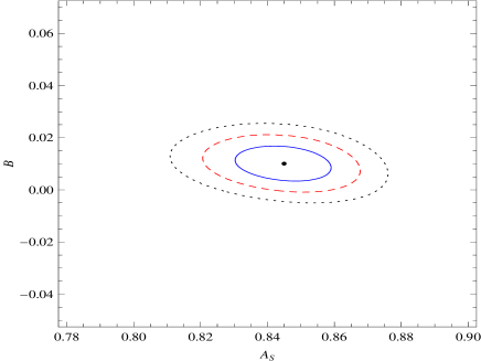
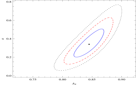
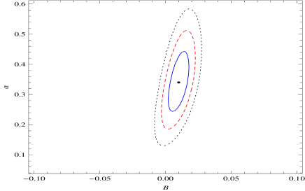
Figure 1: Contours from(i) (H-z)+BAO+CMB+Union2 supernovae data at $68.3$%(Solid) $95.4\%$ (Dashed) and $99.7\%$ (Dotted) confidence limit

3.4 $\chi^{2}$-functions for Supernovae Data

The distance modulus function ($\mu$) is defined in terms of the luminosity distance ($d_{L}$) as

$$\mu(A_{s},B,\alpha,z)=m-M=5\log_{10}(d_{L})+25$$ (3.6)

where

$$d_{L}=\frac{c(1+z)}{H_{0}}\int^{z}_{0}\frac{dz^{\prime}}{E(z^{\prime})}$$ (3.7)

In this case the $\it chi$-square ($\chi^{2}_{\mu}$) function is defined as

$$\chi^{2}_{\mu}(A_{s},B,\alpha,z)=\sum\frac{(\mu(A_{s},B,\alpha,z)-\mu_{obs}(z))^{2}}{\sigma^{2}_{z}}$$ (3.8)

where $\mu_{obs}(z)$ is the observed distance modulus at red shift $z$ and $\sigma_{z}$ is the corresponding error for the observed data[53].

3.5 Combined $\chi^{2}$-function for the Background Tests

Finally the total $\chi^{2}$-function for background tests is defined as follows

$$\chi^{2}_{back}(A_{s},B,\alpha,z)=\chi^{2}_{H-z}(A_{s},B,\alpha,z)+\chi^{2}_{BAO}(A_{s},B,\alpha,z)+\chi^{2}_{CMB}(A_{s},B,\alpha,z)+\chi^{2}_{\mu}(A_{s},B,\alpha,z)$$ (3.9)

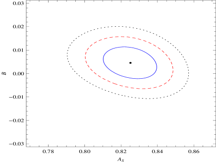
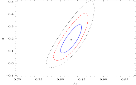
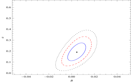
Figure 2: Contours from(i) (H-z)+BAO+CMB+Union2+growth+rms mass fluctuation data at $68.3$%(Solid) $95.4\%$ (Dashed) and $99.7\%$ (Dotted) confidence limit

The $\chi^{2}$ function for the background test is minimized by the present Hubble value predicted by WMAP7. The best fit values of $A_{s}$, $B$, $\alpha$ are thereafter determined.

4 Parametrization of the Growth Index

The growth rate of large scale structures is derived from the matter density perturbation $\delta=\frac{\delta\rho_{m}}{\rho_{m}}$ (where $\delta\rho_{m}$ represents the fluctuation of matter density $\rho_{m}$) in the linear regime which satisfies

$$\ddot{\delta}+2\frac{\dot{a}}{a}\dot{\delta}-4\pi G_{eff}\rho_{m}\delta=0.$$ (4.1)

The field equation for the background cosmology comprising both matter and MCG in FRW universe are given below

$$\left(\frac{\dot{a}}{a}\right)^{2}=\frac{8\pi G}{3}(\rho_{b}+\rho_{mcg}),$$ (4.2)

$$2\frac{\ddot{a}}{a}+\left(\frac{\dot{a}}{a}\right)^{2}=-8\pi G\omega_{mcg}\rho_{mcg}$$ (4.3)

where $\rho_{b}$ represents the background energy density and $\omega_{mcg}$ represents the equation of state for the MCG which is given by

$$\omega_{mcg}=B-\frac{A_{s}(1+B)}{\left[A_{s}+(1-A_{s})(1+z)^{3(1+B)(1+\alpha)})\right]}.$$ (4.4)

We now replace the time $t$ variable in terms of $\ln a$ in eq.(4.1) and obtain

$$(\ln\delta)^{{}^{\prime\prime}}+(\ln\delta)^{{}^{\prime}2}+(\ln\delta)^{{}^{\prime}}\left[\frac{1}{2}-\frac{3}{2}\omega_{mcg}(1-\Omega_{m}(a))\right]=\frac{3}{2}\Omega_{m}(a)$$ (4.5)

where

$$\Omega_{m}(a)=\frac{\rho_{m}}{\rho_{m}+\rho_{mcg}}.$$ (4.6)

The effective matter density is given by $\Omega_{m}=\Omega_{b}+(1-\Omega_{b})(1-A_{s})^{(1/1+\alpha)}$ [54]. Using the energy conservation eq. (2.5) and changing the variable from ${\it ln}a$ to $\Omega_{m}(a)$ once again, the eq. (4.5) can be expressed in terms of the logarithmic growth factor $f=\frac{d\log\delta}{d\log a}$ which is given by

$$3\omega_{mcg}\Omega_{m}(1-\Omega_{m})\frac{df}{d\Omega_{m}}+f^{2}+f\left[\frac{1}{2}-\frac{3}{2}\omega_{mcg}(1-\Omega_{m}(a))\right]=\frac{3}{2}\Omega_{m}(a).$$ (4.7)

The logarithmic growth factor $f$, according to Wang and Steinhardt [13], is given by

$$f=\Omega_{m}^{\gamma}(a)$$ (4.8)

where $\gamma$ is the growth index parameter. In the case of a flat dark energy model with constant equation of state $\omega_{0}$, the growth index $\gamma$ is given by

$$\gamma=\frac{3(\omega_{0}-1)}{6\omega_{0}-5}.$$ (4.9)

For a $\Lambda$CDM model, it reduces to $\frac{6}{11}$ [14, 55], for a matter dominated model, one gets $\gamma=\frac{4}{7}$ [56, 57]. One can also write $\gamma$ as a parametrized function of redshift parameter $z$. One such parametrization is $\gamma(z)=\gamma(0)+\gamma^{{}^{\prime}}z$, with $\gamma^{{}^{\prime}}\equiv\frac{d\gamma}{dz}|_{(z=0)}$ [58, 59]. It has been shown recently [60] that the parametrization smoothly interpolates a low and intermediate redshift range to a high redshift range up to the cosmic microwave background scale. The above parametrization is also taken up in different contexts [61]. In this paper we parametrize $\gamma$ in terms of the MCG parameters namely, $A_{s}$, $\alpha$ and $B$. Therefore, we begin with the following ansatz given by

$$f=\Omega_{m}^{\gamma(\Omega_{m})}(a)$$ (4.10)

where the growth index parameter $\gamma(\Omega_{m})$ can be expanded in a Taylor series around $\Omega_{m}=1$ as

$$\gamma(\Omega_{m})\hskip 227.62204pt$$

$$\;\;\;\;\;\;=\gamma|_{(\Omega_{m}=1)}+(\Omega_{m}-1)\frac{d\gamma}{d\Omega_{m}}|_{(\Omega_{m}=1)}+O(\Omega_{m}-1)^{2}.$$ (4.11)

Consequently eq.(4.7) can be rewritten in terms of $\gamma$ as

$$3\omega_{mcg}\Omega_{m}(1-\Omega_{m})\ln\Omega_{m}\frac{d\gamma}{d\Omega_{m}}-3\omega_{mcg}\Omega_{m}(\gamma-\frac{1}{2})+$$

$$\;\;\;\;\;\Omega_{m}^{\gamma}-\frac{3}{2}\Omega_{m}^{1-\gamma}+3\omega_{mcg}\gamma-\frac{3}{2}\omega_{mcg}+\frac{1}{2}=0.$$ (4.12)

Differentiating once again the above equation around $\Omega_{m}=1$, one obtains zeroth order term in the expansion for $\gamma$ which is given by

$$\gamma=\frac{3(1-\omega_{mcg})}{5-6\omega_{mcg}}.$$ (4.13)

It agrees with a dark energy model for a constant $\omega_{0}$ (eq. 4.9). In the same way differentiating it twice, followed thereafter by a Taylor expansion around $\Omega_{m}=1$, one obtains the first order terms in the expansion which is given by

$$\frac{d\gamma}{d\Omega_{m}}|_{(\Omega_{m}=1)}=\frac{3(1-\omega_{mcg})(1-\frac{3\omega_{mcg}}{2})}{125(1-\frac{6\omega_{mcg}}{5})^{3}}.$$ (4.14)

Substituting it in eq. (4.11), $\gamma$ is obtained, the first order term in this case approximating to

$$\gamma=\frac{3(1-\omega_{mcg})}{5-6\omega_{mcg}}+(1-\Omega_{m})\frac{3(1-\omega_{mcg})(1-\frac{3\omega_{mcg}}{2})}{125(1-\frac{6\omega_{mcg}}{5})^{3}}.$$ (4.15)

Using the expression of $\omega_{mcg}$ in the above, $\gamma$ can be parametrized with the MCG parameters. We define the normalized growth function $g$ from the numerically obtained solution using eq. (4.5) which is given by

$$g(z)\equiv\frac{\delta(z)}{\delta(0)}.$$ (4.16)

The corresponding approximate normalized growth function obtained from the parametrized form of $f$ follows from eq.(4.10) and is given by

$$g_{th}(z)=\exp\left(\int_{1}^{\frac{1}{1+z}}\Omega_{m}(a)^{\gamma}\frac{da}{a}\right).$$ (4.17)

The above expression will be employed once again to construct $\it chi$-square functions in the next section.

4.1 $\chi^{2}$ for growth function (f)

z	$f_{obs}$	$\sigma$	$Ref.$
$0.15$	0.51	0.11	[62, 63]
$0.22$	0.60	0.10	[64]
$0.32$	0.654	0.18	[65]
$0.35$	0.70	0.18	[66]
$0.41$	0.70	0.07	[64]
$0.55$	0.75	0.18	[67]
$0.60$	0.73	0.07	[64]
$0.77$	0.91	0.36	[68]
$0.78$	0.70	0.08	[64]
$1.4$	0.90	0.24	[69]
$3.0$	1.46	0.29	[70]

Table 2: Data for the observed growth functions $f_{obs}$ used in our analysis

z	$\sigma_{8}$	$\sigma_{\sigma_{8}}$	$Ref$
$2.125$	0.95	0.17	[42]
$2.72$	0.92	0.17
$2.2$	0.92	0.16	[43]
$2.4$	0.89	0.11
$2.6$	0.98	0.13
$2.8$	1.02	0.09
$3.0$	0.94	0.08
$3.2$	0.88	0.09
$3.4$	0.87	0.12
$3.6$	0.95	0.16
$3.8$	0.90	0.17
$0.35$	0.55	0.10	[71]
$0.6$	0.62	0.12
$0.8$	0.71	0.11
$1.0$	0.69	0.14
$1.2$	0.75	0.14
$1.65$	0.92	0.20

Table 3: Data for the $\it rms$ mass fluctuations ($\sigma_{8}$) at various redshift

We define $chi$-square for the growth function $f$ as

$$\chi^{2}_{f}(A_{s},B,\alpha,z)=\Sigma\left[\frac{f_{obs}(z_{i})-f_{th}(z_{i},\gamma)}{\sigma_{f_{obs}}}\right]^{2}$$ (4.18)

where $f_{obs}$ and $\sigma_{f_{obs}}$ are obtained from table (2). However, $f_{th}(z_{i},\gamma)$ is obtained from eqs. (4.10) and (4.15). Another observational probe for the matter density perturbation $\delta(z)$ is derived from the red shift dependence of the rms mass fluctuation $\sigma_{8}(z)$. The dispersion of the density field $\sigma^{2}(R,z)$ on a co-moving scale $R$ is defined as

$$\sigma^{2}(R,z)=\int_{0}^{\inf}W^{2}(kR)\Delta^{2}(k,z)\frac{dk}{k}$$ (4.19)

where

$$W(kR)=3\left(\frac{\sin(kR)}{(kR)^{3}}-\frac{\cos(kR)}{(kR)^{2}}\right),$$ (4.20)

represents window function, and

$$\Delta^{2}(kz)=4\pi k^{3}P_{\delta}(k,z),$$ (4.21)

where $P_{\delta}(k,z)\equiv(\delta^{2}_{k})$ is the mass power spectrum at red-shift $z$. The rms mass fluctuation $\sigma_{8}(z)$ is the $\sigma^{2}(R,z)$ at $R=8h^{-1}$ Mpc. The function $\sigma_{8}(z)$ is connected to $\delta(z)$ as

$$\sigma_{8}(z)=\frac{\delta(z)}{\delta(0)}\sigma_{8}|_{(z=0)}$$ (4.22)

which implies

$$s_{th}(z_{1},z_{2})\equiv\frac{\sigma_{8}(z_{1})}{\sigma_{8}(z_{2})}=\frac{\delta(z_{1})}{\delta(z_{2})}=\frac{\exp\left[\int_{1}^{\frac{1}{1+z_{1}}}\Omega_{m}(a)^{\gamma}\frac{da}{a}\right]}{\exp\left[\int_{1}^{\frac{1}{1+z_{2}}}\Omega_{m}(a)^{\gamma}\frac{da}{a}\right]}.$$ (4.23)

In tab-3, a systematic evolution of the rms mass fluctuation $\sigma_{8}(z_{i})$ with observed red shift for flux power spectrum of $\it Ly$-$\alpha$ forest [42, 43, 71] is displayed. In this context we define a new chi-square function which is given by

$$\chi^{2}_{s}(A_{s},B,\alpha,z)=\Sigma\left[\frac{s_{obs}(z_{i},z_{i+1})-s_{th}(z_{i},z_{i+1})}{\sigma_{s_{obs,i}}}\right]^{2}.$$ (4.24)

Data for rms mass fluctuation at various red shift given in table-3 will be considered here. Now considering the growth function mentioned above, one can define a $\it chi$-square function which is given by

$$\chi^{2}_{growth}(A_{s},B,\alpha,z)=\chi^{2}_{f}(A_{s},B,\alpha,z)+\chi^{2}_{s}(A_{s},B,\alpha,z).$$ (4.25)

The $\it chi$-square functions defined above will be considered for the analysis in the next section.

4.2 Combined $\chi^{2}$ function for the background test and growth test

Using eq.(3.9) and eq.(4.25), we define total $\it chi$-square function as

$$\chi^{2}_{total}(A_{s},B,\alpha,z)=\chi^{2}_{back}(A_{s},B,\alpha,z)+\chi^{2}_{growth}(A_{s},B,\alpha,z)$$ (4.26)

where $\chi^{2}_{growth}(A_{s},B,\alpha,z)=\chi^{2}_{f}(A_{s},B,\alpha,z)+\chi^{2}_{s}(A_{s},B,\alpha,z)$. In this case the best fit values are obtained minimizing the $\it chi$-square function. Since the $\it chi$-square function depends on $A_{s}$, $B$, $\alpha$ and $z$, it is possible to draw contours at different confidence limits. The limits imposed by the contours determines the permitted range of values of the EoS parameters in the MCG model.

Data	$A_{s}$	$B$	$\alpha$	$\chi^{2}/d.o.f$
$OHD+BAO+CMB+Union2$	0.8450	0.0101	0.3403	1.0406
$OHD+BAO+CMB+Union2$
$+Growth+\sigma_{8}$	0.8252	0.0046	0.1905	1.0296

Table 4: Best-fit values of the EoS parameters

Data	$CL$	$A_{s}$	$B$
$OHD+BAO+CMB+Union2$	$68.3\%$	$(0.8303,\;0.8593)$	$(0.0034,\;0.0170)$
$OHD+BAO+CMB+Union2$	$95.4\%$	$(0.8202,\;0.8678)$	$(-0.0010,\;0.0212)$
$OHD+BAO+CMB+Union2$	$99.7\%$	$(0.8105,\;0.8762)$	$(-0.0052,\;0.0257)$

Table 5: Range of values of the EoS parameters $A_{s}$ & $B$ from background tests and $OBC=OHD+BAO+CMB$

Data	$CL$	$A_{s}$	$B$
$OBCU+Growth+\sigma_{8}$	$68.3\%$	$(0.8102,\;0.8398)$	$(-0.0023,\;0.0115)$
$OBCU+Growth+\sigma_{8}$	$95.4\%$	$(0.8002,\;0.8488)$	$(-0.0065,\;0.0157)$
$OBCU+Growth+\sigma_{8}$	$99.7\%$	$(0.7906,\;0.8571)$	$(-0.0107,\;0.0203)$

Table 6: Range of values of the EoS parameters $A_{s}$ & $B$ from combined tests and $OBCU=OHD+BAO+CMB+Union2$

Data	$CL$	$A_{s}$	$\alpha$
$OHD+BAO+CMB+Union2$	$68.3\%$	$(0.8184,\;0.871)$	$(0.1988,\;0.5066)$
$OHD+BAO+CMB+Union2$	$95.4\%$	$(0.8024,\;0.8858)$	$(0.1218,\;0.6271)$
$OHD+BAO+CMB+Union2$	$99.7\%$	$(0.7851,\;0.9005)$	$(0.0526,\;0.7708)$

Table 7: Range of values of the EoS parameters $A_{s}$ & $\alpha$ from background tests

Data	$CL$	$A_{s}$	$\alpha$
$OBCU+Growth+\sigma_{8}$	$68.3\%$	$(0.8005,\;0.8492)$	$(0.0821,\;0.3141)$
$OBCU+Growth+\sigma_{8}$	$95.4\%$	$(0.7837,\;0.8642)$	$(0.0212,\;0.4065)$
$OBCU+Growth+\sigma_{8}$	$99.7\%$	$(0.7678,\;0.8793)$	$(-0.0339,\;0.5048)$

Table 8: Range of values of the EoS parameters $A_{s}$ & $\alpha$ from combined tests, and $OBCU=OHD+BAO+CMB+Union2$

Data	$CL$	$B$	$\alpha$
$OHD+BAO+CMB+Union2$	$68.3\%$	$(0.0021,\;0.0175)$	$(0.2433,\;0.4415)$
$OHD+BAO+CMB+Union2$	$95.4\%$	$(-0.0027,\;0.0226)$	$(0.1856,\;0.5107)$
$OHD+BAO+CMB+Union2$	$99.7\%$	$(-0.00816,\;0.0274)$	$(0.1298,\;0.5857)$

Table 9: Range of values of the EoS parameters $B$ & $\alpha$ from background tests

Data	$CL$	$B$	$\alpha$
$OBCU+Growth+\sigma_{8}$	$68.3\%$	$(-0.0034,\;0.0124)$	$(0.1110,\;0.2755)$
$OBCU+Growth+\sigma_{8}$	$95.4\%$	$(-0.0086,\;0.0174)$	$(0.0634,\;0.3332)$
$OBCU+Growth+\sigma_{8}$	$99.7\%$	$(-0.0143,\;0.0222)$	$(0.0187,\;0.3909)$

Table 10: Range of values of the EoS parameters $B$ & $\alpha$ from combined tests and $OBCU=OHD+BAO+CMB+Union2$

Model	$A_{s}$	$B$	$\alpha$	$f$	$\gamma$	$\Omega_{m0}$	$\omega_{0}$	$q(0)$
$MCG$	$0.825$	$0.005$	$0.190$	$0.472$	$0.559$	$0.261$	$-0.836$	$-0.691$
$GCG$	$0.819$	$0.0$	$0.141$	$0.467$	$0.559$	$0.255$	$-0.822$	$-0.684$
$MCG(prev)$	$0.769$	$0.008$	$0.002$	$0.472$	$0.562$	$0.262$	$-0.767$	$-0.607$
$GCG(prev)$	$0.708$	$0.0$	$-0.140$	$0.477$	$0.564$	$0.269$	$-0.708$	$-0.527$
$\Lambda$CDM(prev)	$0.761$	$0.0$	$0.0$	$0.479$	$0.562$	$0.269$	$-0.761$	$-0.603$

Table 11: Values of the EoS parameters in different model

Model	Data	$A_{s}$	$\alpha$	B	$Ref.$
$GCG$	$Supernovae$	0.6-0.85	–	0.0	[73]
$GCG$	$CMBR$	0.81-0.85	0.2-0.6	0.0	[74]
$GCG$	$WMAP$	0.78-0.87	–	0.0	[75]
$GCG$	$CMBR+BAO$	$\approx 0.77$	$\leq 0.1$	0.0	[76]
$MCG$	$OBCU+Growth+\sigma_{8}$	0.825	0.190	0.005	this paper
$MCG$	$Growth+\sigma_{8}+OHD$	0.769	0.002	0.008	[77]

Table 12: Comparison of the values of EoS parameters for GCG and MCG models (using $OBCU=OHD+BAO+CMB+Union2$

5 Summary of the Analysis

The best-fit values of the EoS parameters of the MCG model as determined from the two $\it chi$-squares are shown in Table-4. Contours are drawn for (i) $B$ vs. $A_{s}$ in figs.1(a) and 2(a), (ii) $\alpha$ vs. $A_{s}$ in figs. 1(b) and 2(b), and (iii) $\alpha$ vs. $B$ in figs.1(c) and 2(c) respectively. The allowed ranges of values of the EoS parameters are estimated from the above drawn contours. In Table-5 and 6 the range of values of $A_{s}$ and $B$ from background test and combined tests at different confidence levels are tabulated. We note that $A_{s}$ lies in the interval $(0.8105,\;0.8762)$ and $B$ lies in the interval $(-0.0052,\;0.0257)$ at 3$\sigma$ level in the background test. However, in the combined test, $A_{s}$ and $B$ satisfy the ranges $(0.7906,\;0.8571)$ & $(-0.0107,\;0.0203)$, respectively, at 3$\sigma$ level.

In Table-7 and 8 the allowed ranges of values of $A_{s}$ and $\alpha$ are presented that are obtained from the background test as well as those are obtained from the combined tests at different confidence levels. It is evident that for background test $A_{s}$ and $\alpha$ lie in the intervals $(0.7851,\;0.9005)$ & $(0.0526,\;0.7708)$, respectively at 3$\sigma$ level, whereas the intervals are $(0.7678,\;0.8793)$ & $(-0.0339,\;0.5048)$, respectively, at 3$\sigma$ level in the case of the combined test. In Table-9 and 10 the allowed range of values of $\alpha$ and $B$ are tabulated both for background test and combined tests at different confidence levels. Here, $B$ and $\alpha$ lie in the interval $(-0.00816,\;0.0274)$ & $(0.1298,\;0.5857)$, respectively, at 3$\sigma$ level for background test, whereas they lie in the interval $(-0.0143,\;0.0222)$ & $(0.0187,\;0.3909)$ for the combined tests.

The best-fit values for $A_{s}$, $B$ and $\alpha$ values estimated for background tests are all positive. But in the case of combined test a negative $\alpha$ with positive $A_{s}$ is allowed for $99.7\%$ confidence limit. It is also evident from tables-(9) and (10) that a negative $B$ is also permitted but for a physically viable model we consider $B\geq 0$. The range and the best-fit values for $A_{s}$ is positive in the model.

In fig.-3 the growth function $f$ is plotted with redshift $z$ using best fit values of model parameters. It is evident that the growth function $f$ lies in the range 0.472 to 1.0 for a variation of redshift from $z=0$ to $z=5$. We note that to begin with $f$ remains a constant but decreases sharply at a lower redshift, indicating that the major growth of our universe occurred in the early epoch at a moderate redshift value. In fig.-4 the variation of the growth index $\gamma$ with redshift $z$ is plotted. It is evident that the growth index $\gamma$ varies between 0.559 to 0.60 for a variation of redshift between $z=0$ to $z=5$. A sharp fall in the values of $\gamma$ at low redshift is evident from the figure.
In fig.-5 the variation of the equation of state $\omega$ is plotted with $z$. It is noted that $\omega$ varies from -0.836 at the present epoch ($z=0$) to $\omega\rightarrow 0$ at an intermediate redshift ($z=5$). This result indicates that the universe is now passing through an accelerating phase which is dominated by dark energy whereas in the early universe ($z>5$) it was dominated by matter permitting a decelerating phase.

The variation of the sound speed $c^{2}_{s}$ with redshift $z$ is plotted in fig.-6. It is noted that $c^{2}_{s}$ varies between 0.162 to 0.01 in the above redshift range admitting causality. A small positive value indicates the occurrence of growth in the structures of the universe. The nature of variation of the deceleration parameter is shown in fig-7, which shows that at the present epoch it is $-0.691$ and that there was a decelerating phase in the past as well.

6 Discussion

In the paper we have considered dynamical aspects of the universe considering observational data namely, Stern OHD, CMB shift, BAO peak parameter and supernovae. We also considered here two different growth data sets that are relevant for understanding dark energy making use of MCG as a candidate in an FRW universe. The best-fit values of the parameters $A_{s}$, $B$, $\alpha$ obtained from $\chi^{2}_{tot}(A_{s}$,B,$\alpha)$ are shown in Table-4. Using the best fit values, we analyzed the model and determined the allowed range of values of the EoS parameters which are tabulated in Tables-5,6,7,8,9 and 10. In the case of combined tests, the range of values of $A_{s}$ and $B$ are found to lie in the intervals $(0.7906,\;0.8571)$ & $(-0.0107,\;0.0203)$,respectively, at 3$\sigma$ level, $A_{s}$ and $\alpha$ lie in the intervals $(0.7678,\;0.8793)$ & $(-0.0339,\;0.5048)$, respectively, at 3$\sigma$ level, that of $B$ and $\alpha$ lie in the intervals $(-0.0143,\;0.0222)$ & $(0.0187,\;0.3909)$, respectively. The best-fit values of the growth parameters for the MCG model at the present epoch ($z=0$) is determined which are $f$=0.472, $\gamma$=0.559, $\omega$=-0.836, $q(0)=-0.691$ and $\Omega_{m0}$=0.261 (shown in Table-11). It is also noted that the growth function $f$ varies between 0.472 to 1.0 and the growth index $\gamma$ varies between 0.559 to 0.60 for a variation of redshift from $z=0$ to $z=5$. In this case the equation of state $\omega$ lies between -0.836 to 0 where the sound speed $c_{s}^{2}$ varies between 0.162 to 0.01.

Thus a satisfactory cosmological model is permitted accommodating the present accelerating phase of the universe with MCG in GTR-framework. We note that the range of values for the EoS parameters are considerably different from that obtained in the earlier model [77] when CMB shift,BAO peak parameter and supernovae data were considered. The negative values of the equation of state ($\omega\leq$ -1/3) signifies the existence of such a phase of the universe accommodating acceleration. The sound speed obtained in the model is found small which permits structure formation of the universe. Thus the MCG model may be considered as a good candidate for describing the evolution of the universe which reproduces the cosmic growth with inhomogeneity in addition to a late time accelerating phase.

In Table-11 we present values of the EoS parameters, present growth parameters and density parameter ($\Omega$) for both the MCG and GCG models for comparison. The MCG model is considered as a good fit model with the recent cosmological observations which accommodates recent accelerating phase followed by a decelerating phase. In Table-12, we present values of the EoS parameters corresponding to the previously studied GCG model and MCG models obtained by us. Considering the growth data along with other cosmological observed data, we note that $\alpha$ remains positive number for almost the entire range (Tables-7,8,9,10). The best fit value of the parameter $\alpha$ are positive both for the MCG and GCG models. It is evident that the observational constraints on $\omega$, deceleration parameter and square of sound speed are found considerably higher compared to the previous analysis without the growth test data which indicate structure formation and higher acceleration. Also, it is evident that the present matter contribution is lower (consequently the dark energy contribution is higher) in the current analysis.

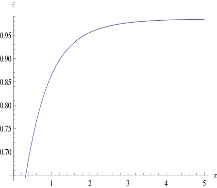
Figure 3: Evolution of growth function $f$ with redshifts in MCG

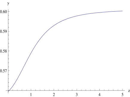
Figure 4: Evolution of growth index $\gamma$ with redshifts in MCG

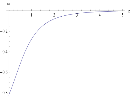
Figure 5: Evolution of the state parameter ($\omega$) in MCG

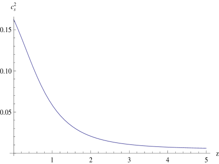
Figure 6: Variation of square of the sound speed in MCG

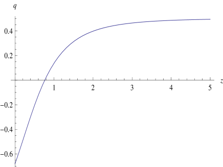
Figure 7: Deceleration parameter with redshift in MCG

It is observed from fig 8 that the model considered here admits an accelerating universe for a positive B ($B\approx 0.005$, a best fit value taken from table-4). It is evident from table 11 that the best fit value of the EoS parameter with MCG ($\omega=-0.84$) lies in the accepted range of values ($-1\leq\omega\leq-0.8$) accommodating accelerating universe. It is noted that a small $c_{s}^{2}$ may be obtained in the model (fig 8) with lower limiting values of $A_{s}$ and $\alpha$ at $99.7\%$ confidence limit taken from tables-(8, 10). For a negative $B$ value ($\approx-0.01$ taken from table-6) a very small value of the sound speed ($\approx 10^{-7}$) which is necessary for adiabatic UDM model is permitted for limiting values of $A_{s}$ and $\alpha$ at $99.7\%$ confidence limit (table-8,10). This UDM can cluster at linear scale. We note that the case with $B<0$ and $A<0$ leads to instability which does not arise in our model as $A=A_{s}(1+B)\rho^{(\alpha+1)}_{0}$ is always positive. It comes out from the analysis that MCG is acceptable which may be used to describe satisfactorily the background tests in cosmology. The shape of the power spectrum in the model obtained from perturbative analysis is shown in fig. (9) for different $A_{s}$ and $\alpha$. It is evident that for a higher value of $\alpha$ and lower $A_{s}$ the spectrum fits well with observational data [78] in MCG. In the MCG model the positivity of the squared sound speed requires both the parameters $B$ and $\alpha$ to be positive definite. It is also noted that a cosmological model with a small range of negative values of B and $\alpha$ can in principle are allowed.
The power spectrum for MCG with observational data [78] is plotted in fig. (9) for various $\alpha$ values to study the stability of the model. Unlike GCG [31] no oscillations in the power spectrum for non-zero $\alpha$ in MCG is observed. In fig -10 we plot the multipole co-efficient $l(l+1)C_{l}/2\pi$ in square microKelvin with l in the case of CMB power spectrum. The solid line drawn corresponds to 3-year WMAP data and different dotted lines are plotted for various values of $\alpha$ $(0,0.01,0.1,0.2,0.3)$ of EoS for MCG. It is evident that for the lower values of $\alpha$ the peak rises and shifts towards the higher l value. It is noted that the CMB power spectrum curve for $\alpha\sim 0.2$ (near the best-fit value of our model), almost matches with the WMAP curve. It is also noted that as $\alpha\rightarrow 0$, the peaks of the power spectrum shifts towards higher l values. Thus a non-zero value of $\alpha$ with MCG describes the observational cosmology. Thus, cosmological model with MCG having non-zero $\alpha$ is found stable unlike GCG where it is unstable.

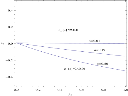
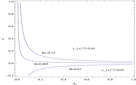
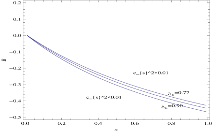
Figure 8: Contours for the adiabatic sound speed

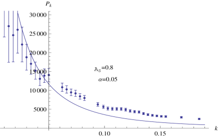
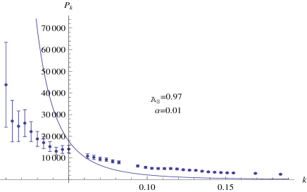
Figure 9: power spectrum in MCG

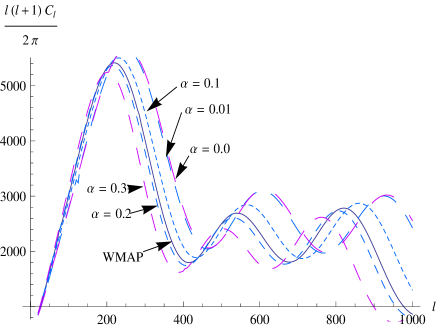
Figure 10: Comparison of the theory with WMAP observations for CMB power spectrum. The solid line corresponds to 3-year WMAP data and dotted lines correspond to $\alpha$ = $(0,0.01,0.1,0.2,0.3)$ of MCG.

7 Acknowledgements

The authors would like to thank the IUCAA Reference Centre at North Bengal University for extending necessary research facilities to initiate the work. BCP would like to thank the Institute of Mathematical Sciences, Chennai for hospitality during a visit and TWAS-UNESCO for awarding Associateship. BCP acknowledges financial support (Major Research Project, Grant No. F. 42-783/2013(SR)) from the University Grants Commission (UGC), New Delhi. PT acknowledges the UGC, New Delhi for financial suport under a Minor Research project (No.F.PSW-073/12-13 (ERO) dated 18.02.13).

References

- [1] S. Perlmutter et al., Nature 391 (1998) 51
- [2] S. Perlmutter et al., Astrophys. J. 517 (1999) 565
- [3] A. G. Riess et al., Astron. J. 116 (1998) 1009
- [4] A. G. Riess et al., Astron. J. 560 (2001) 49
- [5] J. L. Tonry et al., Astrophys. J. 594 (2003) 1
- [6] S. Bridle , O. Lahav , J. P. Ostriker and P. J. Steinhardt Science 299 (2003) 1532
- [7] C.L. Bennett et al., Astrophys. J. Suppl. 148 (2003) 1
- [8] G. Hinshaw et al., Astrophys. J. Suppl. 148 (2003) 135
- [9] A. Kogut et al., Astrophys. J. Suppl. 148 (2003) 161
- [10] D. N. Spergel et al., Astrophys. J. Suppl. 148 (2003) 175
- [11] D. J. Eisenstein et al., Astrophy. J. 633 (2005) 560
- [12] P. J. E. Peebles, ed. Large-Scale Structures of the Universe, (Princeton U. Press, 1980)
- [13] L. Wang and P. J. Steinhardt, Astrophys. J 508 (1998) 483
- [14] E. V. Linder, Phys. Rev. D 72 (2005) 043529
- [15] I. Laszlo and R. Bean, Phys. Rev. D 77 (2008) 024048
- [16] B. Jain and P. Zhang, Phys. Rev. D 78 (2008) 063503
- [17] W. Hu and I.Sawicki, Phys. Rev. D 76 (2007) 104043
- [18] A.Lue, R. Scoccimarro & G. D. Starkman, Phys. Rev. D 69 (2004) 124015
- [19] V. Acquaviva, A. Hajian, D. N. Spergel and S. Das, Phys. Rev. D 78 (2008) 043514
- [20] K. Koyama and R. Maartens , J. Cosmol. Astropart. Phys. 01 (2006) 016
- [21] T. Koivisto and D. F. Mota, Phys. Rev. D 73 (2006) 083502
- [22] S. Daniel , R. Caldwell , A. Cooray and A. Melchiorri, Phys. Rev. D 77 (2008) 103513
- [23] M. Ishak, A. Upadhye and D. N. Spergel, Phys. Rev. D 74 (2006) 043513
- [24] S. Chaplygin, Sci. Mem. Moscow Univ. Math. Phys. 21 (1904) 1
- [25] A. Kamenshchik,U. Moschella and V. Pasquier ,Phys. Lett. B 511 (2001) 265
- [26] Z. H. Zhu Astron. Astrophys., 423 (2004) 421
- [27] M.C. Bento, O. Bertolami and A. A. Sen , Phys. Lett. B 575 (2003) 172
- [28] N. Bilic, G. B.Tupper and R. D. Viollier, Phys. Lett. B 535 (2001) 17
- [29] M. C. Bento, O. Bertolami and A. A. Sen, Phys. Rev. D 66 (2002) 043507
- [30] J.C.Fabris, P.L.C.de Oliveira and H.E.S Velten, Eur. Phys. J. C 71 (2011) 1773
- [31] H. Sandvik, M. Tegmark, M. Zaldarriaga and I. Waga ,Phys. Rev. D 69 (2004) 123524
- [32] L. Amendola, F. Finelli, C. Burigana and D. Caruran , JCAP 0307 (2003) 005
- [33] Lixin Xu, Yuting Wang and Hyerim Noh, Eur. Phys. J. C 72 (2012) 1931
- [34] U. Debnath, A. Banerjee and S. Chakraborty, Class. Quant. Grav. 21 (2004) 5609
- [35] Y. Wu, S. Li, J. Lu and X. Yang, Mod. Phys. Lett. A 22 (2007) 783
- [36] M.L. Bedran, V. Soares and M.E. Araujo, Phys. Lett. B 659 (2008) 462
- [37] S. Costa, M. Ujevic and A.F.dos Santos, Gen Rel. Grav40 (2008) 1683
- [38] U. Debnath and S. Chakraborty , Int. J. Theor. Phys. 47 (2008) 2663
- [39] G. Gupta, S. Sen and A. A. Sen, JCAP 04 (2012) 028
- [40] H. Velten and B.J. Schwarz, JCAP 09 (2011) 016
- [41] E. Hawkins et al., Mon. Not. Roy. Astron. Soc. 346 (2003) 78
- [42] M. Viel, M. G. Haehnelt and V. Spingel, Mon. Not. Roy. Astron. Soc. 354 (2004) 684
- [43] M. Viel and M.G. Haehnelt, Mon. Not. Roy. Astron. Soc. 365 (2006) 231
- [44] N. Kaiser, Astrophys. J. 498 (1998) 26
- [45] A. Mantz, S. W. Allen, H. Ebeling and D. Rapetti, Mon. Not. Roy. Astron. Soc. 387 (2008) 1179
- [46] M. J. Rees and D. W. Sciama, Nature 217 (1968) 511
- [47] L. Amendola, M. Kunz and D. Sapone, JCAP 0804 (2008) 013
- [48] H. Hoekstra et al., Astrophys. J. 647 (2006) 116
- [49] R. G. Crittenden and N.Turok, Phys. Rev. Lett. 76 (1996) 575
- [50] L. Pogosian, P. S. Corasaniti, C. Stephan-Otto, R. Crittenden and R. Nichol, Phys. Rev. D 72 (2005) 103519
- [51] D. Stern, R. Jimenez, L. Verde, M. Kamionkowski and S. Adam Stanford, JCAP 1002 (2010) 008
- [52] E. Komatsu et al., Astrophys. J. Suppl. 192 (2011) 18
- [53] Wang Shuang,Li Xiango-Dong and Li M, Phys. Rev. D 83(2011)023010
- [54] Zhengxiang Li, Puxun Wu and Hongwei Yu, Ap. J. 744 (2012) 176
- [55] E. V. Linder and R. N. Cahn, Astropart. Phys. 28 (2007) 481
- [56] J. N. Fry, Phys. Lett. B 158 (1985) 211
- [57] S. Nesseris and L. Perivolaropoulos, Phys. Rev. D 77 (2008) 023504
- [58] D. Polarski and R. Gannouji, Phys. Lett. B 660 (2008) 439
- [59] R. Gannouji and D. Polarski, JCAP 805 (2008) 018
- [60] M. Ishak and J. Dossett, Phys. Rev. D 80 (2009) 043004
- [61] J. Dossett, M. Ishak, J. Moldenhauer and Y. Gong, A. Wang, JCAP 1004 (2010) 022
- [62] E. Hawkins et al., Mon. Not. Roy. Astron. Soc. 346 (2003) 78; E.V. Linder , Astropart. Phys. 29 (2008) 336
- [63] L. Verde et al., Mon. Not. Roy. Astron. Soc. 335 (2002) 432
- [64] C. Blake et al., Mon. Not. Roy. Astron. Soc. 415 (2011) 2876
- [65] R. Reyes et al., Nature 464 (2010) 256
- [66] M. Tegmark et al., Phys. Rev. D 74 (2006) 123507
- [67] N. P. Ross et al., Mon. Not. Roy. Astron. Soc. 381 (2006) 573
- [68] L. Guzzo et al., Nature 451 (2008) 541
- [69] J. da Angela et al., Mon. Not. Roy. Astron. Soc. 383 (2008) 565
- [70] P. McDonald et al., [SDSS Collaboration] Astrophys. J. 635 (2005) 761
- [71] C. Marinoni et al., A & A 442 (2005) 801
- [72] C. Di Porto and L. Amendola , Phys. Rev. D 77 (2008) 083508
- [73] M. Makler, S.D.de Oliveira and I. Waga , Phys.Lett. B 555 (2003) 1
- [74] M . C. Bento, O. Bertolami and A.A Sen , Phys. Rev. D 67 (2003) 063003
- [75] M . C. Bento, O. Bertolami and A.A Sen , Phys.Lett.B 575 (2003) 172
- [76] T. Barriero, O. Bertolami and P. Torres , Phys. Rev. D 78 (2008) 043530
- [77] B.C.Paul and P. Thakur, JCAP 11 (2013) 052
- [78] S. Cole et al., Mon. Not. Roy. Astron. Soc. 362 (2005) 505