Modeling-based determination of physiological parameters of systemic VOCs by breath gas analysis: a pilot study

Abstract

In this paper we develop a simple two compartment model which extends the Farhi equation to the case when the inhaled concentration of a volatile organic compound (VOC) is not zero. The model connects the exhaled breath concentration of systemic VOCs with physiological parameters such as endogenous production rates and metabolic rates. Its validity is tested with data obtained for isoprene and inhaled deuterated isoprene-D5.

Keywords: Modeling, Breath gas analysis, Volatile organic compounds, Metabolic rates, Production rates, Isoprene, Farhi equation
Version:
J. Breath Res. 9, 036002 (2015).

1 Introduction

The advance of different analytical methods in mass spectrometry within the last twenty years has opened the door to breath gas analysis. There is considerable evidence that volatile organic compounds (VOCs) produced in the human body and then partially released in breath have great potential for diagnosis in physiology and medicine [3]. The emission of such compounds may result from normal human metabolism as well as from pathophysiological disorders, bacterial or mycotic processes (see [1] and the references therein), or exposure to environmental contaminants [20, 21, 27]. As subject-specific chemical fingerprints, VOCs can provide non-invasive and real-time information on infections, metabolic disorders, and the progression of therapeutic intervention.

In a recent paper Spanel et al. [26] investigated the short-term effect of inhaled VOCs on their exhaled breath concentrations. They showed for seven different VOCs that the exhaled breath concentration closely resembles an affine function of the inhaled concentration. This motivated our theoretical investigation regarding the impact of inhaled concentrations for VOCs with low blood:air partition coefficients, i.e., compounds with exhalation kinetics that are described by the Farhi equation [5].

To this extent we develop a simple two compartment model which generalizes the Farhi equation to the case in which the inhaled concentration of a VOC is not negligible. In accordance with the above-mentioned experimental observations, the model predicts that when ventilation and perfusion are kept constant the exhaled breath concentration is indeed an affine function of the inhaled concentration. In addition it links the exhaled breath concentration of systemic VOCs to physiological parameters such as endogenous production rates and metabolic rates, thereby complementing similar efforts in the framework of exposure studies [22, 4]. This estimation process is exemplified by means of exhalation data for endogenous isoprene and inhaled deuterated isoprene-D5.

Another interesting aspect of the model is that for low-soluble VOCs it illustrates a novel approach for answering the question “Is subtracting the inhaled concentration from the exhaled concentration a suitable method to correct measured breath concentrations for room air concentrations?”, an issue that is still being debated within the breath analysis community [19, 23]. In the discussions we indicate how to extend these results to VOCs with higher partition coefficients and how to take into account long-term exposure.
A list of symbols used is provided in Appendix A.

2 A two compartment model

2.1 Derivation of the Farhi equation

To derive the classical Farhi equation which relates alveolar concentrations of VOCs to their underlying blood concentrations one uses a simple two compartment model (see Figure 1) which consists of one single lung compartment and one single body compartment.

Figure 1: Two compartment model consisting of a lung compartment (gas exchange) and a body compartment with production and metabolism. Dashed lines indicate equilibrium according to Henry’s law.

The amount of a VOC transported at time $t$ to and from the lung via blood flow is given by

$$\dot{Q}_{\mathrm{c}}(t)\big{(}C_{\bar{\mathrm{v}}}(t)-C_{\mathrm{a}}(t)\big{)},$$

where $\dot{Q}_{\mathrm{c}}$ denotes the cardiac output, $C_{\bar{\mathrm{v}}}$ is the averaged mixed venous concentration, and $C_{\mathrm{a}}$ is the arterial concentration.

On the other hand, the amount exhaled equals

$$\dot{V}_{\mathrm{A}}(t)\big{(}C_{\mathrm{I}}-C_{\mathrm{A}}(t)\big{)},$$

where $\dot{V}_{\mathrm{A}}$ denotes the ventilation, $C_{\mathrm{I}}$ denotes the concentration in the inhaled air (normally assumed to be zero), and $C_{\mathrm{A}}$ the alveolar air concentration.

This leads to the following mass balance equation describing the change in the concentration of a VOC in the lung (see Figure 2)

$$\tilde{V}_{\mathrm{A}}\frac{dC_{\mathrm{A}}}{dt}=\dot{V}_{\mathrm{A}}(C_{\mathrm{I}}-C_{\mathrm{A}})+\dot{Q}_{\mathrm{c}}(C_{\bar{\mathrm{v}}}-C_{\mathrm{a}}),$$ (1)

where $\tilde{V}_{\mathrm{A}}$ denotes the volume of the lung.

Figure 2: Diagram of gas exchange in an alveoli symbolized by a dashed line.

If the system is in an equilibrium state (e.g., stationary at rest) Equation (1) reads $0=\dot{V}_{\mathrm{A}}\big{(}C_{\mathrm{I}}-C_{\mathrm{A}}(C_{\mathrm{I}})\big{)}+\dot{Q}_{\mathrm{c}}\big{(}C_{\bar{\mathrm{v}}}(C_{\mathrm{I}})-C_{\mathrm{a}}\big{)}$ and using Henry’s law $C_{\mathrm{a}}=\lambda_{\mathrm{b:air}}C_{\mathrm{A}}$ we obtain

$$C_{\mathrm{A}}(C_{\mathrm{I}})=\frac{C_{\mathrm{I}}}{\frac{\lambda_{\mathrm{b:air}}}{r}+1}+\frac{C_{\bar{\mathrm{v}}}(C_{\mathrm{I}})}{\lambda_{\mathrm{b:air}}+r},$$ (2)

where $r=\dot{V}_{A}/\dot{Q}_{c}$ is the ventilation-perfusion ratio and $\lambda_{\mathrm{b:air}}$ denotes the blood:air partition coefficient. The fact is stressed here that $C_{\mathrm{A}}$ and $C_{\bar{\mathrm{v}}}$ depend on the inhaled concentration $C_{\mathrm{I}}$. In particular, this means that if $C_{\mathrm{I}}\not=0$, then subtracting $C_{\mathrm{I}}$ from $C_{\mathrm{A}}$ to arrive at an estimate for $C_{\mathrm{A}}(0)$ will generally give misleading results (more in Subsection 2.3).

Assuming that $C_{\mathrm{I}}=0$ we derive the classical Farhi equation [5]

$$C_{\mathrm{A}}(0)=\frac{C_{\bar{\mathrm{v}}}(0)}{\lambda_{\mathrm{b:air}}+r}.$$ (3)

We summarize the assumptions for the validity of Farhi’s equation and the following extensions:

1. the inhaled concentration is zero, i.e., $C_{I}=0$

2. a stationary state is achieved within the lung, i.e., $\frac{dC_{A}}{dt}=0$

3. the lung behaves uniformly with respect to ventilation and perfusion (a condition that is typically violated in most lung diseases)

4. absorption/desorption phenomena within the upper airways are negligible (i.e., low solubility of the VOC in the airway mucus layer, which is generally fulfilled if $\lambda_{\mathrm{b:air}}<10$, see [2])

5. only alveolar air is sampled so that the alveolar concentration is equal to the exhaled concentration, $C_{\mathrm{A}}=C_{\mathrm{exhaled}}$; in particular, this implies that dead space air contributions have to be avoided, e.g., by CO₂ controlled sampling, and that no airway production (as in the case of NO) takes place

6. no reactions with other breath constituents occur, i.e., the VOC under scrutiny is largely inert

7. the distribution of the blood flow into the different body compartments remains unchanged (e.g., constant at rest)

Note that despite its simplicity, the Farhi equation yields first valuable insights into the exhalation kinetics of VOCs. For instance, the breath concentration of compounds with a low blood:gas partition coefficient $\lambda_{\mathrm{b:air}}$ is expected to react very sensitively to changes of the ventilation-perfusion ratio $r$ (e.g., during exercise, hyperventilation, or breath holding [24]). Typical examples include methane or butane [25, 10].

2.2 Extension of the Farhi equation

To calculate the explicit dependence of $C_{\mathrm{A}}$ and $C_{\bar{\mathrm{v}}}$ on $C_{\mathrm{I}}$ we need to consider the mass balance for the body compartment too. The change of the amount of a VOC in the body is given by the amount which enters the body compartment with the arterial blood plus the amount which is produced in the body minus the amount which is metabolized and the amount leaving via venous blood. Thus the change of the amount of a VOC in the body compartment is given by^,

$$\tilde{V}_{B}\frac{dC_{B}}{dt} =\dot{Q}_{c}(C_{a}-C_{\bar{v}})-\lambda_{b:B}k_{met}C_{B}+k_{prod},$$ (4)

where $k_{met}$ denotes the metabolic rate, $k_{prod}$ the production rate, $\tilde{V}_{B}$ the effective volume of the body, and $C_{B}$ the concentration in the body which is connected to the venous concentration by Henry’s law $C_{\bar{v}}=\lambda_{b:B}\,C_{B}$. Here $\lambda_{b:B}$ denotes the blood:body tissue partition coefficient.

When in an equilibrium state (i.e., $\frac{dC_{\mathrm{A}}}{dt}=0$ and $\frac{dC_{B}}{dt}=0$) we can use Equations (1), (4), and $C_{\bar{v}}=\lambda_{b:B}\,C_{B}$ to eliminate the implicit dependence of $C_{\mathrm{A}}$ on $C_{I}$ in Equation (2)

$$C_{A}(C_{I}) =\frac{\frac{k_{prod}}{k_{met}}}{r+\frac{\dot{V}_{A}}{k_{met}}+\lambda_{\mathrm{b:air}}}+\frac{r+\frac{\dot{V}_{A}}{k_{met}}}{r+\frac{\dot{V}_{A}}{k_{met}}+\lambda_{\mathrm{b:air}}}\,C_{I},$$ (5)

$$C_{\bar{v}}(C_{I}) =\frac{\frac{k_{prod}}{k_{met}}(r+\lambda_{\mathrm{b:air}})}{r+\frac{\dot{V}_{A}}{k_{met}}+\lambda_{\mathrm{b:air}}}+\frac{\frac{\lambda_{\mathrm{b:air}}}{k_{met}}\,r}{r+\frac{\dot{V}_{A}}{k_{met}}+\lambda_{\mathrm{b:air}}}\,C_{I}.$$ (6)

From Equation (5) and (6) we see that the exhaled concentration $C_{A}$ and the mixed venous concentration $C_{\bar{v}}$ solely depend on the inhaled concentration $C_{I}$ and the physiological parameters $k_{prod}$, $k_{met}$, $\dot{V}_{A}$, $\dot{Q}_{c}$, $\lambda_{\mathrm{b:air}}$.

We now discuss some special cases:

1. For $C_{I}=0$ (no trace gas is inspired) this reduces to

   $$C_{A}(0) =\frac{\frac{k_{prod}}{k_{met}}}{r+\frac{\dot{V}_{A}}{k_{met}}+\lambda_{\mathrm{b:air}}},$$

   $$C_{\bar{v}}(0) =\frac{\frac{k_{prod}}{k_{met}}\,(r+\lambda_{\mathrm{b:air}})}{r+\frac{\dot{V}_{A}}{k_{met}}+\lambda_{\mathrm{b:air}}}=C_{A}(0)\,(r+\lambda_{\mathrm{b:air}}).$$ (7)

2. On the other hand, when the production is zero ($k_{prod}=0$), this yields

   $$C_{A}(C_{I}) =\frac{r+\frac{\dot{V}_{A}}{k_{met}}}{r+\frac{\dot{V}_{A}}{k_{met}}+\lambda_{\mathrm{b:air}}}\,C_{I}=\frac{1}{1+\frac{\lambda_{\mathrm{b:air}}}{r+\frac{\dot{V}_{A}}{k_{met}}}}\,C_{I},\quad C_{A}(C_{I})\leq C_{I},$$ (8)

   $$C_{\bar{v}}(C_{I}) =\frac{\frac{\lambda_{\mathrm{b:air}}}{k_{met}}\,r}{r+\frac{\dot{V}_{A}}{k_{met}}+\lambda_{\mathrm{b:air}}}\,C_{I}=\frac{\lambda_{\mathrm{b:air}}}{k_{met}+\dot{Q}_{c}}\,C_{A}(C_{I}).$$ (9)

3. Assuming $C_{\mathrm{A}}=C_{\mathrm{I}}$ (zero alveolar gradient) in Equation (5) yields

   $$C_{I} =\frac{k_{prod}}{k_{met}\,\lambda_{\mathrm{b:air}}}.$$ (10)

2.3 Is subtracing $C_{I}$ a suitable correction method in order to account for inhaled VOC concentrations?

The contribution of room air concentrations to breath concentrations is a long lasting problem in breath gas analysis (see, e.g., [19], [23], [6] and the reviews [16], [18]). In [19], M. Phillips summarized the situation as follows:

Researchers have responded to the problem of room air concentrations with three different strategies:

1. Ignore the problem.

2. Provide the subject with VOC-free air to breathe prior to collection of the breath sample. Unfortunately high quality pure breathing air from commercial sources is usually found to contain a large number of VOCs. In addition it will also contribute to the wash-in/wash-out effect.

3. Correct for the problem by subtracting the background VOCs in room air from the VOCs observed in the breath.

He calls this difference of exhaled concentration and inhaled concentration the alveolar gradient, i.e., it is assumed that $C_{\mathrm{A}}(0)=C_{\mathrm{A}}(C_{\mathrm{I}})-C_{\mathrm{I}}$. To see if this subtraction is correct we consider Equation (5), which we rewrite as

$$C_{A}(C_{I}) =C_{A}(0)+\frac{1}{1+\frac{\lambda_{\mathrm{b:air}}}{r+\frac{\dot{V}_{A}}{k_{met}}}}\,C_{I}.$$

Hence

$$C_{A}(0) =C_{A}(C_{I})-\frac{1}{1+\frac{\lambda_{\mathrm{b:air}}}{r+\frac{\dot{V}_{A}}{k_{met}}}}\,C_{I}.$$ (11)

From this result we conclude that simply subtracting or ignoring the inhaled concentration is generally false. More precisely, for VOCs which fulfill the assumptions made above, $C_{I}$ needs to be multiplied by the following factor

$$a:=\frac{1}{1+\frac{\lambda_{\mathrm{b:air}}}{r+\frac{\dot{V}_{A}}{k_{met}}}}$$ (12)

before subtraction. This factor $a$ is approximately $1$ for small values of $\lambda_{\mathrm{b:air}}$ (e.g., methane, for which $\lambda_{\mathrm{b:air}}<0.1$) or for small values of $k_{met}$ (no metabolism). But it might be $2/3$ if, e.g., $\frac{\lambda_{\mathrm{b:air}}}{r+\frac{\dot{V}_{A}}{k_{met}}}=1/2$.
For perspective, Spanel et al.  experimentally determined $a=0.67$ for isoprene and $a=0.81$ for pentane [26]. Thus one should use the correction $C_{A}(0)=C_{A}(C_{I})-0.67\,C_{I}$ for isoprene and $C_{A}(0)=C_{A}(C_{I})-0.81\,C_{I}$ for pentane.

2.4 Endogenous production and metabolic rates

The question remains how to determine the endogenous production rate and the total metabolic rate of the body using the theoretical framework introduced above. When in a stationary state the averaged values of ventilation and perfusion are constant. Thus Equation (5) resembles a straight line of the form

$$C_{A}(C_{I}) =a\,C_{I}+b,$$ (13)

$C_{I}$ being the variable here. The constants $a$ and $b$ are given by

$$b=C_{A}(0)=\frac{\frac{k_{prod}}{k_{met}}}{r+\frac{\dot{V}_{A}}{k_{met}}+\lambda_{\mathrm{b:air}}}$$ (14)

and

$$a=\frac{(r+\frac{\dot{V}_{A}}{k_{met}})}{r+\frac{\dot{V}_{A}}{k_{met}}+\lambda_{\mathrm{b:air}}}.$$ (15)

Thus the constants $a$ and $b$ are completely determined by the physiological quantities $\dot{V}_{A},\dot{Q}_{c},k_{prod},k_{met}$, and $\lambda_{\mathrm{b:air}}$. The gradient $a$ is independent of $k_{prod}$, fulfills $0<a<1$, and is determined by the metabolic rate $k_{met}$, the ventilation, and perfusion. The quantity $b=C_{A}(0)$ is proportional to the production rate $k_{prod}$.

Varying $C_{I}$, one can measure $C_{A}(C_{I})$ experimentally and thus determine $a$ and $b$. Measuring in addition ventilation and perfusion allows for calculating the total production rate and the total metabolic rate of the body from these two equations

$$k_{prod} =\frac{\frac{b}{1-a}\,\lambda_{\mathrm{b:air}}\,\dot{V}_{A}}{\frac{a}{1-a}\,\lambda_{\mathrm{b:air}}-r},$$ (16)

$$k_{met} =\frac{\dot{V}_{A}}{\frac{a}{1-a}\,\lambda_{\mathrm{b:air}}-r},$$ (17)

or

$$k_{prod} =(\dot{V}_{A}+(r+\lambda_{\mathrm{b:air}})\,k_{met})\,C_{A}(0),$$ (18)

if $k_{met}$ is known.

Remark 1: In [26], Spanel et al. studied the effect of inhaled VOCs on exhaled breath concentrations. Unfortunately, breath frequency and heart rate were not reported. Therefore ventilation and perfusion are unknown and thus $k_{prod}$ and $k_{met}$ cannot be estimated. However, this study shows that Equation (5) explains the experimental findings very well.

Remark 2: This approach yields total endogenous production rates only. As such, one will not be able to determine different production rates in different body compartments. If more than one production source exists, a multi compartment model needs to be set up for the body. Then changes of $r$, e.g., by exercise will vary the fractional blood flows into these compartments, which subsequently allows for estimating compartment-specific production rates.

Remark 3: Due to the term $(-r)$ in the denominator of Equation (17), errors when measuring $a,\dot{V}_{A}$, and $\dot{Q}_{c}$ may cause considerable errors in the rate estimation.

2.5 Changes in production rates

When measuring breath samples or performing ergometer experiments one assumes that the endogenous production rate stays constant during the time frame of these experiments. However, when performing breath analysis during sleep it is possible that the production rate will display, e.g., a circadian rhythm which can be determined by (ventilation and perfusion are considered to be constant)

$$k_{prod}(t)=\big{(}\dot{V}_{A}+(r+\lambda_{\mathrm{b:air}})\,k_{met}\big{)}\,C_{A,0}(t).$$ (19)

3 Experimental findings

In order to validate the present model, end-tidal concentration profiles of endogenous isoprene and inhaled deuterated isoprene-D5 were obtained by means of a real-time setup designed for synchronized measurements of exhaled breath VOCs as well as a number of respiratory and hemodynamic parameters. Our instrumentation has successfully been applied for gathering continuous data streams of these quantities during ergometer challenges [9] as well as in a sleep laboratory setting [8]. These investigations aimed at evaluating the impact of breathing patterns, cardiac output or blood pressure on the observed breath concentration and at studying characteristic changes in VOCs output following variations in ventilation or perfusion. We refer to [9] for an extensive description of the technical details.

In brief, the core of the mentioned setup consists of a head mask spirometer system allowing for the standardized extraction of arbitrary exhalation segments, which subsequently are directed into a Proton-Transfer-Reaction-Time-of-Flight mass spectrometer (PTR-MS-TOF, Ionicon Analytik GmbH, Innsbruck, Austria) for online analysis. (The PTR-MS-TOF replaces the formerly used PTR-MS.) This analytical technique has proven to be a sensitive method for the quantification of volatile molecular species $M$ down to the ppb (parts per billion) range by taking advantage of the proton transfer

$$\mathrm{H_{3}O}^{+}+M\to M\mathrm{H}^{+}+\mathrm{H_{2}O}$$

from primary hydronium precursor ions [14, 15]. Note that this “soft” chemical ionization scheme is selective to VOCs with proton affinities higher than water (166.5 kcal/mol). Count rates of the resulting product ions $M\mathrm{H}^{+}$ or fragments thereof appearing at specified mass-to-charge ratios $m/z$ can subsequently be converted to absolute concentrations of the compound under scrutiny. Specifically, protonated isoprene is detected in PTR-MS-TOF at $m/z=69$, protonated deuterated isoprene-D5 is detected in PTR-MS-TOF at $m/z=74$ and can be measured with breath-by-breath resolution. An underlying sampling interval of 4 s is set for each parameter.

For the experiments, deuterated isoprene-D5 (98%, Campro Scientific GmbH, Germany) was released into the laboratory room with the help of a 0.5-l glass bulb (Supelco, Canada). In a first step, the bulb was evacuated using a vacuum membrane pump and an appropriate volume of liquid isoprene (dependent on the target concentration) was injected through a rubber septum. After complete evaporation of the compound both Teflon valves of the bulb were opened and the bulb content was purged with synthetic air at the flow rate of 1 l/min for 3 minutes. Such conditions provided 3 l of the purge gas (six bulb volumes) to be introduced into the bulb and, thereby, completely displaced the original bulb content. During the bulb purging the laboratory air was continuously mixed with the help of a fan to achieve a homogenous isoprene distribution.

In contrast to chamber experiments the laboratory serves here as a big reservoir (volume: approx. 60 000 l) with a nearly constant background concentration. Three of the authors (one female, two males) took part in five ergometer sessions each (sessions 1–15), at different room air concentrations of deuterated isoprene-D5 (ranging from 30 to 1000 ppb). The exact protocol was as follows (see Figure 3):

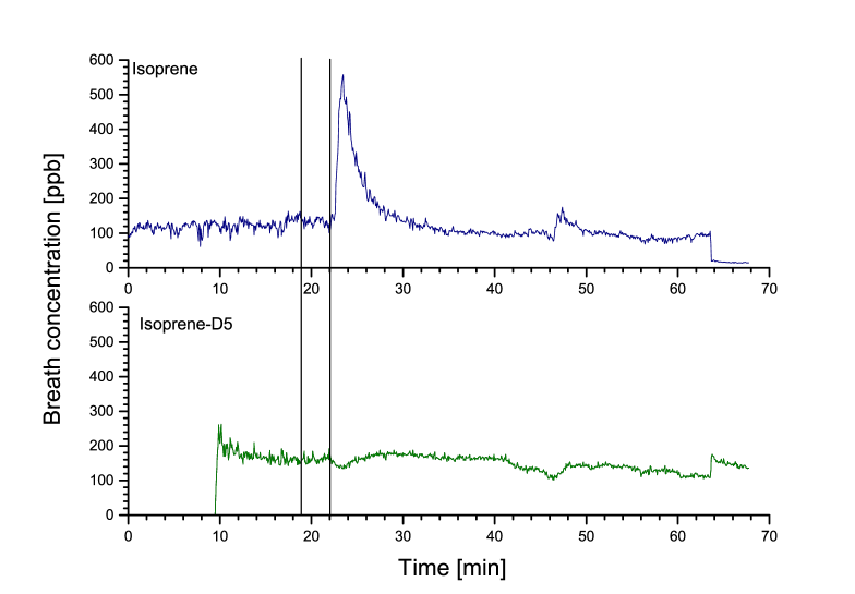
Figure 3: Typical results of a single ergometer session with inhalation of deuterated isoprene-D5: rest for 9 min – release of deuterated isoprene-D5 into the sealed laboratory and waiting for 13 min – 75 Watts for 18 min – rest for 6 min – 75 Watts for 12 min – rest for 5 min; deuterated isoprene-D5 breath concentration: green, normal isoprene breath concentration: blue. In order to validate the 2-compartment model we took the average values at rest from minute 19 to 22 (vertical lines). These values are given in Tables 1 – 3 in column three and four.

• minutes 0–9: the volunteer rests on the ergometer with head-mask on

• minutes 9–12: deuterated isoprene-D5 is released and the room air is mixed by a fan

• minutes 12–22: volunteer rests on the ergometer

• minutes 22–40: volunteer pedals at 75 Watts

• minutes 40–46: volunteer rests on the ergometer

• minutes 46–58: volunteer pedals at 75 Watts

• minutes 58–63: volunteer rests on the ergometer

• minutes 63–68: mask is taken off and the room air concentration is measured.

4 Results

As one can deduce from the prototypical plot in Figure 3, deuterated isoprene-D5 with a partition coefficient of nearly $1$ ($\lambda_{\mathrm{b:air}}=0.95$, [17]) enters the arterial blood stream quickly and it takes only a few minutes until it appears in breath and an equilibrium is achieved in the room air and the blood of the volunteer. To ensure that a steady state was achieved we waited another ten minutes before starting with exercise. At the onset of exercise normal (endogenous) isoprene shows a peak as is well known [9]. This peak presumably stems from a high concentration in muscle blood caused by the production in this compartment [7, 11]. Deuterated isoprene-D5 is nowhere produced in the body. Hence in every compartment of the body its concentration is similar (and zero at the beginning of the experiment). At the onset of exercise, the ventilation-perfusion ratio goes up and the deuterated isoprene-D5 in exhaled breath declines in accordance with the Farhi equation since the venous blood still has an unaltered isoprene level for 1 to 2 minutes (see minute 22 to 24 in Figure 3). But then, due to the increased inhalation of deuterated isoprene-D5, the venous blood gains a higher concentration level (compare with Equation (6)) too and the exhaled concentration of deuterated isoprene-D5 reaches its former level (see minute 24 to 40). For perspective, considering that both isoprene compounds can be assumed to have the same blood:gas partition coefficient $\lambda_{\mathrm{b:air}}$, the profiles in Figure 3 also show that the exercise peak for normal isoprene cannot be explained by changes in ventilation and perfusion alone.

The dynamic behaviour in Figure 3 has mainly been discussed for illustrative purposes. In order to validate the 2-compartment model, only the average resting values of all measured quantities within the last 3 minutes before starting the ergometer challenge were taken into account (minute 19 to 22). These average values are summarized in Tables 1 – 3.

	$C_{I,deuterated}$	$C_{I,normal}$	$C_{A,deuterated}$	$C_{A,normal}$	$\dot{V}_{A}$	$\dot{Q}_{c}$
	[ppb]	[ppb]	[ppb]	[ppb]	[l/min]	[l/min]
Session 1	86.61	11.46	57.06	159.67	6.40	4.53
Session 2	161.88	7.01	131.47	115.12	5.31	4.37
Session 3	202.14	5.16	156.16	100.35	9.56	6.38
Session 4	447.58	8.81	288.41	137.75	8.74	4.66
Session 5	935.78	12.1	390.06	114.79	6.66	4.73
Mean	-	8.91$\pm$2.93	-	125.54$\pm$23.3	7.33$\pm$1.76	4.93$\pm$0.82

Table 1: Volunteer 1 (male, mass: 68 kg, height: 174 cm): normal and deuterated inhaled and exhaled isoprene concentrations with corresponding ventilation and perfusion values.

	$C_{I,deuterated}$	$C_{I,normal}$	$C_{A,deuterated}$	$C_{A,normal}$	$\dot{V}_{A}$	$\dot{Q}_{c}$
	[ppb]	[ppb]	[ppb]	[ppb]	[l/min]	[l/min]
Session 6	49.81	5.48	31.77	45.53	5.75	5.69
Session 7	104.70	6.18	71.62	50.12	5.67	6.11
Session 8	159.72	6.38	106.31	48.73	5.83	5.96
Session 9	226.08	5.74	215.86	48.76	8.95	6.88
Session 10	515.21	7.12	213.93	36.85	8.28	7.48
Mean	-	6.18$\pm$0.63	-	46.0$\pm$5.38	6.9$\pm$1.59	6.42$\pm$0.74

Table 2: Volunteer 2 (female, mass: 62 kg, height: 168 cm): normal and deuterated inhaled and exhaled isoprene concentrations with corresponding ventilation and perfusion values.

	$C_{I,deuterated}$	$C_{I,normal}$	$C_{A,deuterated}$	$C_{A,normal}$	$\dot{V}_{A}$	$\dot{Q}_{c}$
	[ppb]	[ppb]	[ppb]	[ppb]	[l/min]	[l/min]
Session 11	32.09	7.29	22.42	184.59	8.04	4.46
Session 12	68.08	6.07	44.91	180.69	8.06	4.79
Session 13	127.22	6.37	87.93	190.25	8.65	4.54
Session 14	164.33	5.90	137.19	142.16	7.28	4.40
Session 15	617.11	7.81	351.69	170.88	8.13	4.09
Mean	-	6.69$\pm$0.83	-	173.71$\pm$19.0	8.03$\pm$0.49	4.46$\pm$0.25

Table 3: Volunteer 3 (male, mass: 90 kg, height: 180 cm): normal and deuterated inhaled and exhaled isoprene concentrations with corresponding ventilation and perfusion values.

From Tables 1 – 3 we are able calculate the metabolic rates for deuterated isoprene-D5 for each volunteer. To this end, we perform a nonlinear least square optimization using Equation (8)

$$\sum\left(\frac{C_{A}(C_{I})}{C_{I}}-\frac{(r+\frac{\dot{V}_{A}}{k_{met}})}{r+\frac{\dot{V}_{A}}{k_{met}}+\lambda_{\mathrm{b:air}}}\right)^{2}\longrightarrow\min$$ (20)

The sum is taken over the respective sessions for each volunteer here, thereby yielding individual values for $k_{met}$. The results are listed in Table 4.

	Volunteer 1	Volunteer 2	Volunteer 3
$k_{\mathrm{met}}$	$16.87\pm 4.8$	$7.95\pm 4.0$	$22.63\pm 4.8$

Table 4: Metabolic rates (in [l/min]) for deuterated isoprene-D5 for each volunteer.

Since normal isoprene and deuterated isoprene-D5 behave similarly from a chemical standpoint, we assume, neglecting isotopic effects, as a first approximation that both have the same metabolic rate.

Using the average resting ventilation $\dot{V}_{A}$, the average resting perfusion $\dot{Q}_{c}$, and the metabolic rates in Table 4, we may thus compute the gradient $a$ by Equation (15), and the corrected average exhaled normal isoprene concentration $C_{\mathrm{A}}(0)=C_{\mathrm{A}}(C_{\mathrm{I}})-a\,C_{\mathrm{I}}$. By employing Equation (18) we can then calculate the corresponding endogenous production rate for normal isoprene. The results are listed in Table 5.

	$\dot{Q}_{c}$	$\dot{V}_{A}$	$a$	$C_{\mathrm{A}}(0)$	$k_{\mathrm{prod}}$
	[l/min]	[l/min]		ppb	[nmol/min]
Volunteer 1	4.93	7.33	0.669	120.6	216.4
Volunteer 2	6.42	6.9	0.671	41.9	35.7
Volunteer 3	4.46	8.03	0.694	169.0	439.9

Table 5: Production rates for isoprene for each volunteer (with $V_{mol}=27$ l).

As an additional remark, one can also calculate the total production rate $k_{prod}$ and the total metabolic rate $k_{met}$ from the three compartment model presented in[7] by combining the two body compartments (richly perfused and peripheral compartment)

$$k_{prod}=k_{\mathrm{pr}}^{\mathrm{rpt}}+k_{\mathrm{pr}}^{\mathrm{per}},\quad k_{met}=\frac{k_{\mathrm{met}}^{\mathrm{rpt}}\lambda_{\mathrm{b:rpt}}C_{\mathrm{rpt}}+k_{\mathrm{met}}^{\mathrm{per}}\lambda_{\mathrm{b:per}}C_{\mathrm{per}}}{C_{\bar{\mathrm{v}}}}.$$

Here $k_{\mathrm{pr}}^{\mathrm{rpt}},k_{\mathrm{pr}}^{\mathrm{per}}$ denote the production rates in the richly perfused and peripheral compartment, $\lambda_{\mathrm{b:rpt}},\lambda_{\mathrm{b:per}}$ the corresponding partition coefficients, and $C_{\mathrm{rpt}},C_{\mathrm{per}}$ the corresponding concentrations.

Taking the nominal values from Table 2 and Table C1 in [7] yields $k_{met}=10$ l/min and $k_{prod}=125.3$ nmol/min, which is similar to the values extracted above.

5 Discussion

In this paper we developed the conceptually simplest compartment model for systemic VOCs that can be described by the Farhi equation in terms of their exhalation kinetics. In particular, a special focus is given to the case when the inhaled (e.g., ambient air) concentration is significantly different from zero. The model elucidates a novel approach for computing metabolic/production rates of systemic VOCs with low blood:air partition coefficients from the respective breath concentrations. Moreover, it clarifies how breath concentration of such VOCS should be corrected when the inhaled concentration cannot be neglected. The model predictions with respect to an affine relationship between exhaled breath concentrations and inhaled concentrations are in excellent agreement with measurements by Spanel et al. [26].

Nevertheless, a number of limitations should be mentioned here. Firstly, in order to apply this model for the estimation of metabolic/production rates, further studies with a representative number of patients will be necessary. In particular, the individual and population ranges of these quantities will have to be determined. In addition, it should be investigated how these parameters vary with age, body mass, sex, etc.. To circumvent the intricate measurements of ventilation and perfusion, one could use heart frequency and breath frequency.

In order to account for long-term exposure, the model should be extended to incorporate a storage compartment which fills up and depletes according to its partition coefficient. This yields then a 3-compartment model. For instance, Pleil et al.  demonstrated in [21] that a 3-compartment model suffices to model the long-term elimination (over 35 hours) of trichloroethylene after exposure. However, for short-term exposure experiments as carried out in Section 3, the influence of such a storage compartment will merely be reflected by a slightly different metabolic rate.

When there is an influence of the upper airway walls (i.e., for highly hydrophilic VOCs), the exhaled concentration deviates considerably from the alveolar concentration, i.e., $C_{\mathrm{exhaled}}\not=C_{A}$. In that case the lung must be modeled by at least two compartments [12] or more [2]. In addition breath concentrations will become flow and temperature dependent. Due to this fact, for hydrophilic VOCs one also would have to resort to alternative sampling approaches such as isothermal rebreathing to extract the underlying alveolar concentration [13]. Also, the formulas for metabolic rates and endogenous production rates will be different.

Appendix A List of symbols

Parameter	Symbol
cardiac output	$\dot{Q}_{\mathrm{c}}$
averaged mixed venous concentration	$C_{\bar{\mathrm{v}}}$
arterial concentration	$C_{\mathrm{a}}$
ventilation	$\dot{V}_{\mathrm{A}}$
inhaled air concentration	$C_{\mathrm{I}}$
alveolar air concentration	$C_{\mathrm{A}}$
lung volume	$\tilde{V}_{\mathrm{A}}$
blood:air partition coefficient	$\lambda_{\mathrm{b:air}}$
ventilation-perfusion ratio	$r$
exhaled concentration	$C_{\mathrm{exhaled}}$
metabolic rate	$k_{met}$
production rate	$k_{prod}$
effective volume of the body	$\tilde{V}_{B}$
body concentration	$C_{B}$
blood:body partition coefficient	$\lambda_{b:B}$
inhaled air concentration of normal isoprene	$C_{I,normal}$
inhaled air concentration of isoprene-D5	$C_{I,deuterated}$
alveolar air concentration of isoprene-D5	$C_{A,deuterated}$
alveolar air concentration of normal isoprene	$C_{A,normal}$
production rate in the richly perfused compartment	$k_{\mathrm{pr}}^{\mathrm{rpt}}$
production rate in the peripheral compartment	$k_{\mathrm{pr}}^{\mathrm{per}}$
blood:richly perfused compartment partition coefficient	$\lambda_{\mathrm{b:rpt}}$
blood:peripheral compartment partition coefficient	$\lambda_{\mathrm{b:per}}$
richly perfused compartment concentration	$C_{\mathrm{rpt}}$
peripheral compartment concentration	$C_{\mathrm{per}}$

References

References

- [1] A. Amann and D. Smith (eds.), Volatile Biomarkers, Elsevier, Boston, 2013.
- [2] J. C. Anderson, A. L. Babb, and M. P. Hlastala, Modeling soluble gas exchange in the airways and alveoli, Ann. Biomed. Eng. 31 (2003), 1402–22.
- [3] B. de Lacy Costello, A. Amann, H. Al-Kateb, C. Flynn, W. Filipiak, T. Khalid, D. Osborne, and N. M. Ratcliffe, A review of the volatiles from the healthy human body, J. Breath Res. 8 (2014), no. 1, 014001.
- [4] G. A. Csanády and J. G. Filser, Toxicokinetics of inhaled and endogenous isoprene in mice, rats, and humans, Chem. Biol. Interact. 135-136 (2001), 679–85.
- [5] L. E. Farhi, Elimination of inert gas by the lung, Respiration physiology 3 (1967), no. 1, 1–11.
- [6] J. Herbig and J. Beauchamp, Towards standardization in the analysis of breath gas volatiles, J. Breath Res. 8 (2014), no. 3, 037101.
- [7] J. King, H. Koc, K. Unterkofler, P. Mochalski, A. Kupferthaler, G. Teschl, S. Teschl, H. Hinterhuber, and A. Amann, Physiological modeling of isoprene dynamics in exhaled breath, J. Theor. Biol. 267 (2010), 626–37.
- [8] J. King, A. Kupferthaler, B. Frauscher, H. Hackner, K. Unterkofler, G. Teschl, H. Hinterhuber, A. Amann, and B. Högl, Measurement of endogenous acetone and isoprene in exhaled breath during sleep, Physiol. Meas. 33 (2012), no. 3, 413.
- [9] J. King, A. Kupferthaler, K. Unterkofler, H. Koc, S. Teschl, G. Teschl, W. Miekisch, J. Schubert, H. Hinterhuber, and A. Amann, Isoprene and acetone concentration profiles during exercise on an ergometer, J. Breath Res. 3 (2009), 027006 (16pp).
- [10] J. King, P. Mochalski, A. Kupferthaler, K. Unterkofler, H. Koc, W. Filipiak, S. Teschl, H. Hinterhuber, and A. Amann, Dynamic profiles of volatile organic compounds in exhaled breath as determined by a coupled PTR-MS/GC-MS study, Physiol. Meas. 31 (2010), 1169–1184.
- [11] J. King, P. Mochalski, K. Unterkofler, G. Teschl, M. Klieber, M. Stein, A. Amann, and M. Baumann, Breath isoprene: muscle dystrophy patients support the concept of a pool of isoprene in the periphery of the human body, Biochem. Biophys. Res. Commun. 423 (2012), 526–530.
- [12] J. King, K. Unterkofler, G. Teschl, S. Teschl, H. Koc, H. Hinterhuber, and A. Amann, A mathematical model for breath gas analysis of volatile organic compounds with special emphasis on acetone, J. Math. Biol. (2011), 959–999.
- [13] J. King, K. Unterkofler, G. Teschl, S. Teschl, P. Mochalski, H. Koc, H. Hinterhuber, and A. Amann, A modeling based evaluation of isothermal rebreathing for breath gas analysis of highly soluble volatile organic compounds, J. Breath Res. 6 (2012), 016005.
- [14] W. Lindinger, A. Hansel, and A. Jordan, On-line monitoring of volatile organic compounds at pptv levels by means of proton-transfer-reaction mass spectrometry (PTR-MS) – Medical applications, food control and environmental research, Int. J. Mass Spectrometry 173 (1998), 191–241.
- [15] , Proton-transfer-reaction mass spectrometry (PTR-MS): on-line monitoring of volatile organic compounds at pptv levels, Chem. Soc. Rev. 27 (1998), 347–354.
- [16] C. Lourenco and C. Turner, Breath analysis in disease diagnosis: Methodological considerations and applications, Metabolites 4 (2014), no. 2, 465–498.
- [17] P. Mochalski, J. King, A. Kupferthaler, K. Unterkofler, H. Hinterhuber, and A. Amann, Measurement of isoprene solubility in water, human blood and plasma by multiple headspace extraction gas chromatography coupled with solid phase microextraction, J. Breath Res. 5 (2011), no. 4, 046010.
- [18] J. Pereira, P. Porto-Figueira, C. Cavaco, K. Taunk, S. Rapole, R. Dhakne, H. Nagarajaram, and J. S. Camara, Breath analysis as a potential and non-invasive frontier in disease diagnosis: An overview, Metabolites 5 (2015), no. 1, 3–55.
- [19] M. Phillips, J. Herrera, S. Krishnan, M. Zain, J. Greenberg, and R. Cataneo, Variation in volatile organic compounds in the breath of normal humans, J. Chromatogr. B. Biomed. Sci. Appl. 729 (1999), 75–88.
- [20] J. Pleil and M. Stiegel, Evolution of environmental exposure science: Using breath-borne biomarkers for discovery of the human exposome, Analytical Chemistry 85 (2013), no. 21, 9984–9990, PMID: 24067055.
- [21] J. Pleil, M. Stiegel, and T. Risby, Clinical breath analysis: discriminating between human endogenous compounds and exogenous (environmental) chemical confounders, J. Breath Res. 7 (2013), 017107.
- [22] J. D. Pleil, D. Kim, J. D. Prah, D. L. Ashley, and S. M. Rappaport, The unique value of breath biomarkers for estimating pharmacokinetic rate constants and body burden from environmental exposures, Breath Analysis for Clinical Diagnosis and Therapeutic Monitoring (A. Amann and D. Smith, eds.), World Scientific, Singapore, 2005, pp. 347–359.
- [23] J. K. Schubert, W. Miekisch, T. Birken, K. Geiger, and G. F. E. Nöldge-Schomburg, Impact of inspired substance concentrations on the results of breath analysis in mechanically ventilated patients, Biomarkers 10 (2005), 138–152.
- [24] P. Sukul, P. Trefz, J. K. Schubert, and W. Miekisch, Immediate effects of breath holding maneuvers onto composition of exhaled breath, J. Breath Res. 8 (2014), no. 3, 037102.
- [25] A. Szabo, V. Ruzsany, K. Unterkofler, A. Mohacsi, E. Tuboly, M. Boros, G. Szabo, and A. Amann, Exhaled methane concentration profiles during exercise on an ergometer, J. Breath Res. 9 (2015), 016009.
- [26] P. Španěl, K. Dryahina, and D. Smith, A quantitative study of the influence of inhaled compounds on their concentrations in exhaled breath, J. Breath Res. 7 (2013), no. 1, 017106.
- [27] L. Wallace, E. Pellizzari, and G. Sydney, A linear model relating breath concentrations to environmental exposures: application to a chamber study of four volunteers exposed to volatile organic chemicals, J. Expo. Anal. Environ. Epidemiol. 3 (1993), 75 –102.