Bose-Einstein condensate strings

Abstract

We consider the possible existence of gravitationally bound general relativistic strings consisting of Bose-Einstein condensate (BEC) matter which is described, in the Newtonian limit, by the zero temperature time-dependent nonlinear Schrödinger equation (the Gross-Pitaevskii equation), with repulsive interparticle interactions. In the Madelung representation of the wave function, the quantum dynamics of the condensate can be formulated in terms of the classical continuity equation and the hydrodynamic Euler equations. In the case of a condensate with quartic nonlinearity, the condensates can be described as a gas with two pressure terms, the interaction pressure, which is proportional to the square of the matter density, and the quantum pressure, which is without any classical analogue though, when the number of particles in the system is high enough, the latter may be neglected. Assuming cylindrical symmetry, we analyze the physical properties of the BEC strings in both the interaction pressure and quantum pressure dominated limits, by numerically integrating the gravitational field equations. In this way we obtain a large class of stable stringlike astrophysical objects, whose basic parameters (mass density and radius) depend sensitively on the mass and scattering length of the condensate particle, as well as on the quantum pressure of the Bose-Einstein gas.

I Introduction

The observation, in 1995, of Bose-Einstein condensation in dilute alkali gases, such as vapors of rubidium and sodium, confined in a magnetic trap and cooled to very low temperatures exp , represented a major breakthrough in experimental condensed matter physics, as well as a major confirmation of an important prediction in theoretical statistical physics. At very low temperatures, all particles in a dilute Bose gas condense to the same quantum ground state, forming a Bose-Einstein condensate (BEC), which appears as a sharp peak over a broader distribution in both coordinate and momentum space. Particles become correlated with each other when their wavelengths overlap, that is, when the thermal wavelength $\lambda_{T}$ is greater than the mean interparticle distance $l$. This happens at a critical temperature $T_{c}<2\pi\hbar^{2}n^{2/3}/mk_{B}$, where $m$ is the mass of an individual condensate particle, $n$ is the number density, and $k_{B}$ is Boltzmann’s constant Da99 ; rev ; Ch05 ; Pit ; Pet ; Zar . A coherent state develops when the particle density is high enough, or the temperature is sufficiently low. From an experimental point of view, the condensation is indicated by the generation of a sharp peak in the velocity distribution, which is observed below the critical temperature exp . More recently, quantum degenerate gases have been created by a combination of laser and evaporative cooling techniques, opening several new lines of research at the border of atomic, statistical and condensed matter physics Da99 ; rev ; Ch05 ; Pit ; Pet ; Zar .

Since Bose-Einstein condensation is a phenomenon that has been observed and well studied in the laboratory, the possibility that it may occur on astrophysical or cosmic scales cannot be rejected a priori. Thus, dark matter, which is required to explain the dynamics of the neutral hydrogen clouds at large distances from the Galactic center, and which is a cold bosonic system, could also exist as a Bose-Einstein condensate Sin . In fact, since there exists a formal analogy between classical scalar fields and BECs, any theory of scalar field dark matter may also be viewed as condensate system SF-BEC . In early studies, such as those given in Sin , either a phenomenological approach was adopted, or the solutions of the Gross-Pitaevskii equation, which describes the condensate in the nonrelativistic limit, were investigated numerically. A systematic study of the properties of condensed galactic dark matter halos was performed in BoHa07 and these systems have been further investigated by numerous authors inv .

By introducing the Madelung representation of the wave function, the dynamics of the dark matter halo can be formulated in terms of the continuity equation and the hydrodynamic Euler equations. Hence, condensed dark matter can be described as a Newtonian gas, whose density and pressure are related by a barotropic equation of state. However, in the case of a condensate with quartic nonlinearity, the equation of state is polytropic with index $n=1$ BoHa07 .

Furthermore, though superfluids, such as liquid ⁴He, are far from being dilute, there is, nevertheless, good reason to believe that the phenomenon of superfluidity is related to that of Bose-Einstein condensation. Both experimental observations and theoretical calculations estimate the condensate fraction at $T=0$ (denoted $n_{0}$) for superfluid helium to be around $n_{0}\approx 0.10$ and, since a strongly correlated pair of fermions can be treated approximately like a boson, the arising superfluidity can be interpreted as the condensation of coupled fermions. Similarly, the transition to a superconducting state in a solid material may be described as the condensation of electrons or holes into Cooper pairs, which drastically reduces the friction caused by the flow of current Ch05 .

The possibility of Bose-Einstein condensation in nuclear and quark matter has also been considered in the framework of the so-called Bardeen-Cooper-Schrieffer to Bose-Einstein condensate (BCS-BEC) crossover BCS-BEC . At ultrahigh density, matter is expected to form a degenerate Fermi gas of quarks in which Cooper pairs of quarks form a condensate near the Fermi surface (a color superconductor csc ). If the attractive interaction is strong enough, at some critical temperature the fermions may condense into the bosonic zero mode, forming a quark BEC Bal95 . In general, fermions exist in a BCS state when the attractive interaction between particles is weak. The system then exhibits superfluidity, characterized by the energy gap for single-particle excitations which is created by the formation of the Cooper pairs. Conversely, a BEC exists when the attractive interaction between fermions is strong, causing them to first form bound “molecules” (i.e. bosons), before starting to condense into the bosonic zero mode at some critical temperature. An important point is that the BCS and BEC states are smoothly connected, without a phase transition between the two (NiAb05, ) (see also Sun:2007fc ; He:2007kd ; He:2007yj ; He:2010nb ; He:2013gga for additional work on the BCS-BEC crossover in relativistic matter).

Remarkably, the critical temperature in the BEC region is, in fact, independent of the precise strength of the coupling for the attractive interaction between fermions. This is because an increase in the coupling strength affects only the internal structure of the bosons, whereas the critical temperature is determined by their kinetic energy. Thus, the critical temperature reaches an upper limit for strong coupling, as long as the effect of the binding energy on the total mass of the boson is small, and can be neglected. In this limit, we are able to use a nonrelativistic framework to describe the BCS-BEC crossover (NiAb05, ).

However, in relativistic systems, the binding energy makes a significant contribution to the total mass of the boson and cannot be neglected. In this case, two crossovers are possible. First, an ordinary BCS-BEC crossover may occur, though the critical temperature in the BEC region no longer tends towards an upper bound, due to relativistic effects. Second, the nonrelativistic BEC state undergoes a transition to a relativisitc BEC (RBEC) state, in which the critical temperature increases to the order of the Fermi energy (NiAb05, ).

The possibility of Bose condensates existing in neutron stars has been considered (see Glendenning Gl00 for a detailed discussion), as the condensation of negatively charged mesons in neutron star matter is favored, since these mesons would replace electrons with very high Fermi momenta. Recently, Bose-Einstein condensates of kaons/anti-kaons in compact objects were also discussed BaBa03 ; Ban04 . Pion as well as kaon condensates would have two important effects on neutron stars. First, condensates soften the equation of state above the critical density for the onset of condensation, which reduces the maximal possible neutron star mass. At the same time, however, the central stellar density increases, due to the softening. Second, meson condensates would lead to neutrino luminosities which are considerably enhanced over those of normal neutron star matter. This would speed up neutron star cooling considerably (Gl00, ). Another particle which may form a condensate is the H-dibaryon, a doubly strange six-quark composite with zero spin and isospin, and baryon number $B=2$. In neutron star matter, which may contain a significant fraction of $\Lambda$ hyperons (i.e. neutral subatomic hadrons consisting of one up, one down and one strange quark, labeled $\Lambda^{0}$) LambdaHyperon , these particles could combine to form H-dibaryons Hdibar . Thus, H-matter condensates may thus exist at the center of neutron stars (Gl00, ). Neutrino superfluidity, as suggested by Kapusta Ka04 , may also lead to Bose-Einstein condensation (Ab06, ).

These results show that the possibility of the existence of Bose-Einstein condensed matter inside compact astrophysical objects, or even the existence of stars formed entirely from a BEC, cannot be excluded a priori. The properties of BEC stars have been considered in ChHa , and it was shown that these hypothetical astrophysical objects have mass and radii ranges that are compatible with the observed physical parameters of some neutron stars. Bearing this in mind, it is the purpose of the current paper to consider another possible astrophysical BEC system, with potentially important cosmological implications, namely, the Bose-Einstein condensate string. By this, we mean a cylindrically symmetric system consisting of bosonic matter in a Bose-Einstein condensed phase.

The structure of this paper is then as follows. In Sec. II, we briefly review the general treatment of gravitationally bound Bose-Einstein condensates in the nonrelativistic limit, including their description by the generalized Gross-Pitkaevskii equation (Sec. II.1) and the hydrodynamical representation (Sec. II.2) in which a quantum potential term, which is significant close to the boundary of the condensate, arises. Using the nonrelativistic analysis as a guide, we determine that the thermodynamic (“interaction”) pressure of BEC dark matter is governed by a polytropic equation of state which, together with the assumption of cylindrical symmetry, allows us to fix the general form of the metric, and of the components of the energy-momentum tensor, which are expressed in terms of the energy density and pressure of the fluid. The latter is, in turn, decomposed into interaction and quantum pressure terms, denoted $p$ and $p_{Q}$, respectively, and the two limiting cases $p\gg p_{Q}$ and $p_{Q}\gg p$ are considered separately. Thus, the string geometry and the corresponding form of the Einstein field equations are determined in Sec. III and, by appropriately redefining the relevant dynamical variables, these are then recast (in each limiting case) as an autonomous system of differential equations, which may be solved numerically. Specifically, Sec. III.1 reviews the semiclassical approximation for the relativistic treatment of the quantum pressure term and Sec. III.2 deals with the string geometry and components of Einstein tensor, while the numerical solutions of the field equations for interaction dominated and quantum pressure dominated strings are given in Secs. III.3 and III.4, respectively. The meaning and significance of the variation, with respect to the radial coordinate $r$, of the physical parameters of the BEC string (i.e. the three-dimensional energy density and pressure, and the mass per unit length) and of the components of the metric tensor that determine the resulting space-time, is discussed, in each limiting case, at the end of the relevant subsection. In Sec. III.5 we carefully consider the effects of the geometry of the space-time on the quantum pressure term. The physical parameters of the string are obtained by numerically integrating the field equations for a fixed set of initial conditions, and for different values of the single free model parameter. The comparison of the two quantum string models is considered and, by analyzing and discussing the behavior of the physical and geometrical quantities, we estimate the effect of the geometry on the global properties of the string. Finally, Sec. IV contains a brief treatment of BEC strings in the Newtonian approximation of the gravitational field, from which it is seen that constraints on the order of magnitude values of physically important quantities can be easily obtained. A summary of the results for both the thermodynamic and quantum pressure dominated regimes, together with some brief remarks regarding their possible cosmological and astrophysical significance, and suggestions for future work, are given in Sec. V.

II Bose-Einstein Condensation

In a quantum system of $N$ interacting condensed bosons, most of the bosons lie in the same single-particle quantum state. For a system consisting of a large number of particles, the calculation of the ground state of the system with the direct use of the Hamiltonian is impracticable, due to the high computational cost. However, the use of some approximate methods can lead to a significant simplification of the formalism. One such approach is the mean field description of the condensate, which is based on the idea of separating out the condensate contribution to the bosonic field operator. We also assume that, in a medium composed of scalar particles with nonzero mass, when the transition to a Bose-Einstein condensed phase occurs, the range of Van der Waals-type scalar mediated interactions among particles becomes infinite.

II.1 The Gross-Pitaevskii equation

The many-body Hamiltonian describing interacting bosons confined by an external potential $V_{ext}$ is given, in the second quantization, by

$$\hat{H}=\int d\vec{r}\hat{\Phi}^{+}\left(\vec{r}\right)\left[-\frac{\hbar^{2}}{2m}\vec{\nabla}^{2}+V_{ext}\left(\vec{r}\right)\right]\hat{\Phi}\left(\vec{r}\right)+$$

$$\frac{1}{2}\int d\vec{r}d\vec{r}^{\prime}\hat{\Phi}^{+}\left(\vec{r}\right)\hat{\Phi}^{+}\left(\vec{r}^{\prime}\right)V_{int}\left(\vec{r}-\vec{r}^{\prime}\right)\hat{\Phi}\left(\vec{r}\right)\hat{\Phi}\left(\vec{r}^{\prime}\right),$$ (1)

where $\vec{\nabla}$ is the three-dimensional Laplacian, $\hat{\Phi}\left(\vec{r}\right)$ and $\hat{\Phi}^{+}\left(\vec{r}\right)$ are the boson field operators that annihilate and create a particle at the position $\vec{r}$, respectively, and $V_{int}\left(\vec{r}-\vec{r}^{\prime}\right)$ is the two-body interatomic potential Da99 ; Ch05 ; Pet . $V_{ext}\left(\vec{r}\right)$ represents an “externally applied” potential. However, in the nonrelativistic limit, Newtonian gravitational potentials, even those corresponding to the gravitational field of the condensate itself, may be considered as externally applied potentials in this sense.

In order to simplify this formalism, we now adopt the mean field approximation and separate out the contribution to the bosonic field operator. For a uniform gas in a volume $\mathcal{V}$, a BEC forms in the single-particle state $\Phi_{0}=1\sqrt{\mathcal{V}}$, having zero momentum. The field operator can then be decomposed as $\hat{\Phi}\left(\vec{r}\right)=\sqrt{\mathcal{N}/\mathcal{V}}+\hat{\Phi}^{\prime}\left(\vec{r}\right)$, where $\mathcal{N}$ is the total number of particles in the condensate. By treating the operator $\hat{\Phi}^{\prime}\left(\vec{r}\right)$ as a small perturbation, one can develop the first-order theory for the excitations of the interacting Bose gases Da99 ; Ba01 .

In the general case of a nonuniform and time-dependent configuration the field operator in the Heisenberg representation is given by $\hat{\Phi}\left(\vec{r},t\right)=\psi\left(\vec{r},t\right)+\hat{\Phi}^{\prime}\left(\vec{r},t\right)$, where $\psi\left(\vec{r},t\right)$, also called the condensate wave function, is the expectation value of the field operator, $\psi\left(\vec{r},t\right)=\left\langle\Psi|\hat{\Phi}\left(\vec{r},t\right)|\Psi\right\rangle$. It is a classical field, and its absolute value fixes the number density of the condensate particles according to $\rho_{\mathcal{N}}\left(\vec{r},t\right)=\left|\psi\left(\vec{r},t\right)\right|^{2}$. The normalization condition is $\mathcal{N}=\int\rho_{\mathcal{N}}\left(\vec{r},t\right)d^{3}\vec{r}$.

The equation of motion for the condensate wave function is the Heisenberg equation corresponding to the many-body Hamiltonian given by Eq. (II.1),

$$i\hbar\frac{\partial}{\partial t}\hat{\Phi}\left(\vec{r},t\right)=\left[\hat{\Phi},\hat{H}\right]=\left[-\frac{\hbar^{2}}{2m}\vec{\nabla}^{2}+V_{ext}\left(\vec{r}\right)\right.+$$

$$\left.\int d\vec{r}^{\prime}\hat{\Phi}^{+}\left(\vec{r}^{\prime},t\right)V_{int}\left(\vec{r}^{\prime}-\vec{r}\right)\hat{\Phi}\left(\vec{r}^{\prime},t\right)\right]\hat{\Phi}\left(\vec{r},t\right).$$ (2)

The zeroth-order approximation to the Heisenberg equation is obtained by replacing $\hat{\Phi}\left(\vec{r},t\right)$ with the condensate wave function $\psi\left(\vec{r},t\right)$. In the integral containing the particle-particle interaction, $V_{int}\left(\vec{r}^{\prime}-\vec{r}\right)$, this replacement is, in general, a poor approximation for short distances. However, in a dilute and cold gas, only binary collisions at low energy are relevant, and these collisions are characterized by a single parameter, the $s$-wave scattering length $l_{s}$, independently of the details of the two-body potential. Therefore, one can replace $V_{int}\left(\vec{r}^{\prime}-\vec{r}\right)$ with an effective interaction $V_{int}\left(\vec{r}^{\prime}-\vec{r}\right)=u_{0}\delta\left(\vec{r}^{\prime}-\vec{r}\right)$, where $u_{0}=4\pi\hbar^{2}l_{s}/m$, $l_{s}$ is the coherent scattering length (defined as the zero-energy limit of the scattering amplitude, $l_{s}=\lim_{T\rightarrow 0}f_{scat}$, and $m$ is the mass of an individual condensate particle. With the use of the effective potential the integral in the bracket of Eq. (2) gives $u_{0}\left|\psi\left(\vec{r},t\right)\right|^{2}$, and the resulting equation is the Schrödinger equation with a quartic nonlinear term Da99 ; rev ; Pit ; Pet ; Zar ; BoHa07 . This gives the generalized Gross-Pitaevskii equation, describing a gravitationally trapped Bose-Einstein condensate in the nonrelativistic limit,

$$i\hbar\frac{\partial}{\partial t}\psi\left(\vec{r},t\right) = \bigg{[}-\frac{\hbar^{2}}{2m}\vec{\nabla}^{2}+V_{ext}\left(\vec{r}\right)+$$ (3)

$$u_{0}\left|\psi\left(\vec{r},t\right)\right|^{2}\bigg{]}\psi\left(\vec{r},t\right).$$

As for $V_{ext}\left(\vec{r}\right)$, we assume that it is the Newtonian gravitational potential, which we denote as $V_{grav}$, which satisfies the Poisson equation

$$\vec{\nabla}^{2}V_{grav}=4\pi G\rho,$$ (4)

where $\rho=m\rho_{\mathcal{N}}=m\left|\psi\left(\vec{r},t\right)\right|^{2}$ is the mass density inside the condensate.

II.2 The hydrodynamical representation

The physical properties of a Bose-Einstein condensate described by the generalized Gross-Pitaevskii equation, Eq. (3), can be understood much more easily using the so-called Madelung representation of the wave function Da99 , which here consists of writing $\psi\left(\vec{r},t\right)$ in the form

$$\psi\left(\vec{r},t\right)=\sqrt{\frac{\rho\left(\vec{r},t\right)}{m}}\exp\left[\frac{i}{\hbar}S\left(\vec{r},t\right)\right],$$ (5)

where the function $S\left(\vec{r},t\right)$ has the dimensions of an action. Substituting the above expression for $\psi\left(\vec{r},t\right)$ into Eq. (3), the latter decouples into a system of two differential equations for the real functions $\rho$ and $\vec{v}$, given by

$$\frac{\partial\rho}{\partial t}+\vec{\nabla}\cdot\left(\rho\vec{v}\right)=0,$$ (6)

$$\rho\left[\frac{\partial\vec{v}}{\partial t}+\left(\vec{v}\cdot\vec{\nabla}\right)\vec{v}\right] = -\vec{\nabla}P\left(\frac{\rho}{m}\right)-\rho\vec{\nabla}\left(\frac{V_{ext}}{m}\right)-\rho\vec{\nabla}V_{Q},$$

where we have introduced the quantum potential

$$V_{Q}=-\frac{\hbar^{2}}{2m}\frac{\vec{\nabla}^{2}\sqrt{\rho}}{\sqrt{\rho}},$$ (8)

the velocity of the quantum fluid, defined as

$$\vec{v}=\frac{\vec{\nabla}S}{m},$$ (9)

and have denoted

$$P\left(\rho\right)=U_{0}\rho^{2},$$ (10)

where

$$U_{0} = \frac{2\pi\hbar^{2}l_{s}}{m^{3}}=$$

$$1.232\times 10^{50}\left(\frac{m}{1\;\mathrm{meV}}\right)^{-3}\left(\frac{l_{s}}{10^{9}\;\mathrm{fm}}\right)\;\mathrm{cm}^{5}/\mathrm{g}\;\mathrm{s}^{2},$$

or

$$U_{0}=0.1856\times 10^{5}\left(\frac{l_{s}}{1\;\mathrm{fm}}\right)\left(\frac{m}{2m_{n}}\right)^{-3},$$ (12)

where $m_{n}=1.6749\times 10^{-24}$ g is the mass of the neutron.

Therefore, the equation of state of the Bose-Einstein condensate with quartic nonlinearity is a polytrope with index $n=1$. However, in the case of low-dimensional systems Kolo it has been shown that, in many experimentally interesting cases, the nonlinearity will be cubic, or even logarithmic in $\rho$.

From its definition it follows that the velocity field is irrotational, satisfying the condition $\vec{\nabla}\times\vec{v}=0$. Therefore the equations of motion for the gravitationally bound, ideal Bose-Einstein condensate (in the nonrelativistic limit), take the form of the continuity equation plus the hydrodynamic Euler equation, with the density and pressure related by a barotropic equation of state Da99 ; Ch05 ; Pet .

By taking into account the mathematical identity

$$\tau\vec{\nabla}\left(\frac{\vec{\nabla}^{2}\sqrt{\tau}}{\sqrt{\tau}}\right)=\frac{1}{2}\vec{\nabla}\left(\tau\vec{\nabla}^{2}\ln\tau\right),$$ (13)

which holds for any dimensionless scalar function $\tau$, it follows that the quantum potential $V_{Q}$ generates a quantum pressure $p_{Q}$, given in a general form as Da99 ; Ch05 ; Pet

$$p_{Q}=\frac{\rho\vec{\nabla}V_{Q}}{\hbar^{2}}=-\frac{\hbar^{2}}{4m^{2}}\rho\vec{\nabla}^{2}\ln(\rho/\rho_{c}),$$ (14)

where $\rho_{c}$ is the central density of the BEC mass distribution. This pressure can have a significant effect for small particle masses and high densities.

When the number of particles becomes large enough, the quantum pressure term makes a significant contribution only near the boundary of the condensate. Hence it is much smaller than the nonlinear interaction term. Thus, the quantum stress term in the equation of motion for the condensate can be neglected. This is the Thomas-Fermi approximation, which has been used extensively for the study of Bose-Einstein condensates Da99 ; Ch05 ; Pet . As the number of particles in the condensate becomes infinite, the Thomas-Fermi approximation becomes exact. This approximation also corresponds to the classical limit of the theory, i.e. to neglecting all terms in nonzero powers of $\hbar$, or, equivalently, to the regime of strong repulsive interactions among particles. In the hydrodynamical representation, the Thomas-Fermi approximation corresponds to neglecting all terms containing $\vec{\nabla}{\rho}$ (or $\vec{\nabla}\sqrt{\rho}$) and $\vec{\nabla}{S}$ in the equations of motion.

For cylindrical distributions, such as those considered (relativistically) in the remainder of this study, the corresponding equation of motion in the nonrelativistic limit is the “cylindrical Lane-Emden equation”, $\left(1/\xi\right)d\left(\xi d\theta/d\xi\right)/d\xi+\theta^{n}=0$, which is equivalent to $\left(1/\xi\right)d\left((\xi/n)(d\tau/d\xi)\tau^{\frac{1}{n}-1}\right)/d\xi+\tau=0$, where $\theta^{n}=\tau=\rho/\rho_{c}$, for finite $n$, where $\rho_{c}$ is the central density at $r=0$. For a barotropic fluid, the limit $n\rightarrow\infty$ must be taken before substituting the equation of state into the Poisson equation, leading to the separate (critical) case, for which $\left(1/\xi\right)d\left(\xi d(\ln(\tau))/d\tau\right)/d\xi+\tau=0$. In this case, we have that $\Gamma\rightarrow 2$, $\alpha\rightarrow U_{0}$ and $\xi=[U_{0}/(4\pi G\rho_{c})]^{1/2}r$. This equation can also be generalized to include rotating fluids by adding a term of the form $\Omega^{2}\xi$, where $\Omega=\Omega(\xi)$ is a function of the rescaled radial coordinate $\xi$ only, to the right-hand side Ostriker(1964) ; Schneider+Schmitz(1995) ; Christodoulou+Kazanas(2007) .
Hence, all Bose-Einstein condensate forms of matter can generally be described as fluids satisfying a polytropic equation of state of index $n$ and, importantly, this remains true relativistically, as well as in the nonrelativistic limit, which, in effect, has been thoroughly studied in Ostriker(1964) ; Schneider+Schmitz(1995) ; Christodoulou+Kazanas(2007) , at least in the limit of the Fermi-Thomas approximation. The remainder of this study is therefore dedicated to determining the astrophysical and cosmological significance of stringlike (i.e. cylindrically symmetric) BEC dark matter structures, by studying them in a general relativistic context. For simplicity, we consider only the case of the condensates with quartic nonlinearity since, in this case, the physical properties of the condensate are relatively well known from laboratory experiments and can be described in terms of only two free parameters, the mass $m$ of the condensate particle, and the scattering length $l_{s}$.

III Static Bose-Einstein condensate strings in cylindrically symmetric geometries

In this section we consider the properties of a string consisting of matter in a Bose-Einstein condensed state. In the hydrodynamical description of the condensate the equilibrium properties of this system are determined by two physical parameters, the interaction pressure $p$, and the quantum pressure $p_{Q}$, respectively. In the following we will investigate two classes of BEC strings, corresponding to the conditions $p>>p_{Q}$ (interaction energy dominated strings), and $p_{Q}>>p$ (quantum pressure dominated strings).

III.1 General relativistic Bose-Einstein condensates - the semiclassical approximation

In formulating our initial, general relativistic, model of gravitationally bound Bose-Einstein condensates, we consider that bosonic matter at temperatures below the critical temperature $T_{c}$ represents a hybrid system, in which the gravitational field remains classical, while the bosonic condensate is described by quantum fields in which gravitational effects induced by the non-Euclidian space-time geometry can be effectively neglected. In the standard approach used for coupling quantum fields to a classical gravitational field (i.e. semiclassical gravity), the energy-momentum tensor that serves as the source in the Einstein equations is replaced by the expectation value of the energy-momentum operator $\hat{T}_{\mu\nu}$, with respect to some quantum state $\Psi$ Carl ,

$$R_{\mu\nu}-\frac{1}{2}g_{\mu\nu}R=\frac{8\pi G}{c^{4}}\left\langle\Psi\left|\hat{T}_{\mu\nu}\right|\Psi\right\rangle,$$ (15)

where $R_{\mu\nu}$ is the Ricci tensor, $R$ is the scalar curvature, and $g_{\mu\nu}$ is the metric tensor of the space-time. In the nonrelativistic limit, the state function $\Psi$ evolves according to the Gross-Pitaevski equation and $\Psi\rightarrow\psi$ so that, for a quartic nonlinear term, the evolution of the condensate wave function $\psi$ is determined by Eq. (3), with $V_{ext}$ being given by the gravitational potential $V_{grav}$, which is the Newtonian limit of Eq. (15) for a cylindrically symmetric system. Hence, in the semiclassical approach, we obtain

$$\left\langle\Psi\left|\hat{T}_{\mu\nu}\right|\Psi\right\rangle\approx\left\langle\psi\left|\hat{T}_{\mu\nu}\right|\psi\right\rangle=T_{\mu\nu},$$ (16)

as the source term in the Einstein field equations, where $T_{\mu\nu}$ is the effective energy-momentum tensor of the condensate system obtained from the Gross-Pitaevskii equation. In a comoving frame $T_{\mu\nu}$ is diagonal with components

$$T_{\mu\nu}=\left(\rho c^{2},-P,-P,-P\right),$$ (17)

where $\rho c^{2}$ denotes the three-dimensional energy density and $P$ denotes the total effective thermodynamic pressure of the system, obtained from the hydrodynamic representation. That is, $P\approx p+p_{Q}$, where $p$ is the genuine classical (interaction) thermodynamic pressure and $p_{Q}$ is the quantum pressure term, as discussed previously. Therefore, in the first approximation, we can assume that the effective thermodynamic properties (energy density and pressure) of the Bose-Einstein condensed matter are given by the relations derived from the quantum Gross-Pitaevskii equation in the Newtonian approximation of the gravitational field and in a standard Euclidian quantum geometry. However, geometric effects may play an important role in the equation of state of the quantum string, and we will consider the effects these may have on Eq. (14) by appropriately defining the operator $\vec{\nabla}^{2}$ in the given Riemannian geometry.

III.2 Geometry and gravitational field equations of Bose-Einstein condensate strings

For the geometrical description of Bose-Einstein condensate strings we adopt cylindrical polar coordinates $(x^{0}=t,x^{1}=r,x^{2}=\phi,x^{3}=z)$ and assume a cylindrically symmetric metric, which gives rise to a line element of the form clv

$$ds^{2}=g_{\mu\nu}dx^{\mu}dx^{\nu}=N^{2}(r)dt^{2}-d{r}^{2}-L^{2}(r)d{\phi}^{2}-K^{2}(r)dz^{2},$$ (18)

where $N(r)$, $L(r)$ and $K(r)$ are arbitrary functions of the radial coordinate $r$. The nonzero Christoffel symbols associated to the metric (18) are given by

$$\Gamma_{rt}^{t}=\frac{N^{\prime}(r)}{N(r)},\Gamma_{tt}^{r}=N(r)N^{\prime}(r),\Gamma_{r\phi}^{\phi}=\frac{L^{\prime}(r)}{L(r)},$$

$$\Gamma_{\phi\phi}^{r}=-L(r)L^{\prime}(r),\Gamma_{rz}^{z}=\frac{K^{\prime}(r)}{K(r)},\Gamma_{zz}^{r}=-K(r)K^{\prime}(r),$$

where a prime denotes the derivative with respect to $r$, and the nonzero components of the Ricci tensor are clv

$$R_{t}^{t} = \frac{(LKN^{\prime})^{\prime}}{NLK},R_{r}^{r}=\frac{N^{\prime\prime}}{N}+\frac{L^{\prime\prime}}{L}+\frac{K^{\prime\prime}}{K},$$ (20)

$$R_{\phi}^{\phi}=\frac{(NKL^{\prime})^{\prime}}{NLK},R_{z}^{z}=\frac{(NLK^{\prime})^{\prime}}{NLK}.$$

III.3 Interaction energy dominated Bose-Einstein condensate strings

In this section, we assume that the quantum pressure term inside the BEC string is negligible. This corresponds to the Thomas-Fermi approximation, which is valid when the number of particles is very large. However, in the context of a cylindrically symmetric distribution, we must remember that the term large refers to the number of particles present in a thin, effectively two-dimensional slice of the string, i.e. a perpendicular cross section, rather than the total number within the string as a whole. As such, it is unlikely that this assumption will hold with any degree of accuracy for very narrow strings and, in general, we would expect the ratio of the string surface area to its internal volume to play a significant role in its dynamics, especially for narrow stings in which the “boundary region” occupies a significant proportion of the overall volume. In other words, we would expect the internal quantum dynamics of the string to play a significant role in determining its macroscopic (essentially classical) dynamics, through the generation of an effective surface tension.

As an immediate corollary, we see that, were we to attempt to derive an effective action for a BEC string, it would not be possible to simply take the “wire approximation” (i.e. the zero thickness limit Anderson ; topological_defects ), as used, for example, to derive the Nambu-Goto action NambuGoto as the effective action for Nielsen-Olesen strings no . Rather, we would need to develop a modified Nambu-type action (such as those corresponding to species of chiral, superconducting, or current-carrying string, e.g. in NiOl87 ; BlOlVi01 ; CoHiTu87 ), incorporating surface tension effects, possibly through the existence of an additional rigidity and/or elasticity terms (c.f. Anderson et al.(1997) ; Gregory(1988) ; Gregory(1988)* ). Though such an analysis remains beyond the scope of the current paper, it would form the next logical step in the study of BEC strings HarkoLake2014 . In principle, for strings in which the thermodynamic pressure $p$ and quantum pressure $p_{Q}$ are both significant (which are not considered in the present study), both finite-thickness corrections (c.f. MaedaTurok(1988) ) and surface tension effects may also need to be incorporated.

However, within the limit of the Thomas-Fermi approximation, the Bose-Einstein condensate can be described as a quantum gas satisfying a polytropic equation of state with index $n=1$. Therefore, the source term in the field equations is given by the energy-momentum tensor of a BEC, with the following components

$$T_{t}^{t}=\rho(r)c^{2},T_{r}^{r}=T_{\phi}^{\phi}=T_{z}^{z}=-p(r).$$ (21)

We then have

$$T=T_{\mu}^{\mu}=\rho(r)c^{2}-3p(r),p(r)=U_{0}\rho^{2}(r),$$ (22)

and the field equations describing cylindrically symmetric string-type solutions in general relativity,

$$R_{\mu\nu}=\frac{8\pi G}{c^{4}}\left(T_{\mu\nu}-\frac{1}{2}Tg_{\mu\nu}\right),$$ (23)

can be written as

$$\frac{(LKN^{\prime})^{\prime}}{NLK}=\frac{4\pi G}{c^{4}}\left(\rho c^{2}+3p\right),$$ (24)

$$\frac{N^{\prime\prime}}{N}+\frac{L^{\prime\prime}}{L}+\frac{K^{\prime\prime}}{K}=\frac{4\pi G}{c^{4}}\left(p-\rho c^{2}\right),$$ (25)

$$\frac{(NKL^{\prime})^{\prime}}{NLK}=\frac{4\pi G}{c^{4}}\left(p-\rho c^{2}\right),$$ (26)

$$\frac{(NLK^{\prime})^{\prime}}{NLK}=\frac{4\pi G}{c^{4}}\left(p-\rho c^{2}\right).$$ (27)

Generally, the regularity of the geometry on the symmetry axis is imposed via the initial conditions,

$$L(0)=0,L^{\prime}(0)=1,N(0)=1,N^{\prime}(0)=0.$$ (28)

Next, we consider the relations that follow from the conservation of the energy-momentum tensor, given by Eq. (21). Since all the components of the energy-momentum tensor are independent of the coordinates $t$, $\phi$ and $z$, the relations

$$\nabla_{\mu}T_{t}^{\mu}=0,\nabla_{\mu}T_{\phi}^{\mu}=0,\nabla_{\mu}T_{z}^{\mu}=0$$ (29)

hold automatically. Furthermore, the divergence of $T_{\nu}^{\mu}$ can be obtained in a general form as LaLi

$$\nabla_{\mu}T_{\nu}^{\mu}=\frac{1}{\sqrt{-g}}\frac{\partial}{\partial x^{\mu}}\left(\sqrt{-g}T_{\nu}^{\mu}\right)-\frac{1}{2}\frac{\partial g_{\alpha\beta}}{\partial x^{\nu}}T^{\alpha\beta}.$$ (30)

It follows that Eqs. (29) are identically satisfied, with the only potentially nonzero component of the divergence of the energy-momentum tensor being given by

$$\nabla_{\mu}T_{r}^{\mu}=\frac{1}{\sqrt{-g}}\frac{d}{dr}\left(\sqrt{-g}T_{r}^{r}\right)-\frac{1}{2}\frac{\partial g_{\alpha\beta}}{\partial r}T^{\alpha\beta}=0,$$ (31)

where $\sqrt{-g}=NKL$ and $\alpha=\beta\in\left\{r,\phi,z\right\}$ for our choice of metric in Eq. (18), and energy-momentum tensor, Eq. (21).

Substituting Eq. (21) into Eq. (31), the conservation equation for the BEC string takes the form

$$\frac{dp}{dr}+\left(\rho c^{2}+p\right)\frac{N^{\prime}}{N}=0.$$ (32)

An upper bound for the density of the string arises from imposing the trace energy condition $T=\rho c^{2}-3p\geq 0$, which restricts the range of allowed densities to

$$\rho\leq\frac{c^{2}}{3U_{0}}.$$ (33)

To describe the physical characteristics of the BEC string, we introduce the Tolman mass per unit length within the radius $r$ (hereafter, we will often use the phrase Tolman mass to refer to the Tolman mass per unit length), $M(r)$, defined as

$$M(r)=\frac{1}{c^{2}}\int{\left(\rho c^{2}-3U_{0}\rho^{2}\right)\sqrt{-g}d^{2}x}=$$

$$2\pi\int_{r^{\prime}=0}^{r}{\left[\rho\left(r^{\prime}\right)-3\frac{U_{0}}{c^{2}}\rho^{2}\left(r^{\prime}\right)\right]N\left(r^{\prime}\right)L\left(r^{\prime}\right)K\left(r^{\prime}\right)dr^{\prime}}.$$

The total Tolman mass of the string is defined as $M=\lim_{r\rightarrow R_{s}}M\left(r\right)$, where $R_{s}$ is the radius of the string, which defines the vacuum boundary. We also introduce the parameter $W(r)$, which can be related to the physical deficit angle in the space-time of the string, and which is defined as Verbin

$$W(r)=-\frac{2\pi}{c^{2}}\int\left(\rho c^{2}-p\right)\sqrt{-g}d^{2}x=$$

$$-2\pi\int_{r^{\prime}=0}^{r}\rho\left(r^{\prime}\right)\left[1-\frac{U_{0}}{c^{2}}\rho\left(r^{\prime}\right)\right]N\left(r^{\prime}\right)L\left(r^{\prime}\right)K\left(r^{\prime}\right)dr^{\prime}.$$

On the vacuum boundary of the string the function $W(r)$ has the finite value $W=\lim_{r\rightarrow R_{s}}W(r)$. By assuming that the string can extend to infinity, so that $R_{s}\rightarrow\infty$, and that the asymptotic form of the metric for the Bose-Einstein Condensate string is flat, from the field equations, Eqs. (24)-(27), together with the definitions for $M$ and $W$, it follows that

$$\left[N^{\prime}LK\right]_{r=0}^{\infty} = 2GM,$$ (36)

$$\left[NL^{\prime}K\right]_{r=0}^{\infty} = 2GW,$$ (37)

$$\left[NLK^{\prime}\right]_{r=0}^{\infty} = 2GW,$$ (38)

and

$$\frac{L^{\prime}}{L}\bigg{|}_{r=0}^{\infty}=\frac{K^{\prime}}{K}\bigg{|}_{r=0}^{\infty}.$$ (39)

We then have

$$L^{\prime}(\infty)=\frac{2GW+K(0)}{N(\infty)K(\infty)},$$ (40)

for $L^{\prime}(0)=N(0)=1$, and the angular deficit in the cylindrical geometry, due to the presence of the string, is given by Verbin

$$\Delta\phi=2\pi(1-L^{\prime}(\infty)),$$ (41)

which can be numerically estimated by substituting values of $N(r)$ and $K(r)$, for large $r$. However, in order to do this for strings of finite width, we would require a precise knowledge of the vacuum solution surrounding the string core. The general form of this solution is well known: it is the Kasner solution, which is the unique, cylindrically symmetric vacuum solution in general relativity Kasner ; Harvey ; exact-sol but, for the sake brevity, we treat only the interior solution for the BEC string in this paper. In order to estimate the angular deficit using the formula given in Eq. (41), we would therefore need to match the Kasner space-time onto the interior solution at the string boundary, $r=R_{s}$ (defined as the point beyond which the energy and pressure density vanish, or become negative, so that $\rho c^{2}(R_{s})=p(R_{s})=0$), thereby fixing the numerical values of the Kasner parameters, before taking the limit $r\rightarrow\infty$ to determine $L^{\prime}(\infty)$. As a first approximation, however, we may substitute $L^{\prime}(R_{s})$ into Eq. (41), in place of $L^{\prime}(\infty)$, and use the formula

$$\Delta\phi\approx 2\pi(1-L^{\prime}(R_{s})),$$ (42)

from which we can obtain an order of magnitude estimate of the deficit angle in the exterior BEC string geometry, using the numerical solutions of the field equations for the string interior.

For the sake of notational simplicity, we now introduce the variables

$$\sqrt{-g}=\Sigma=NLK,\ H_{t}=\frac{N^{\prime}}{N},H_{\phi}=\frac{L^{\prime}}{L},\ H_{z}=\frac{K^{\prime}}{K},$$ (43)

and

$$H=\frac{1}{3}\left(H_{t}+H_{\phi}+H_{z}\right)=\frac{1}{3}\frac{\Sigma^{\prime}}{\Sigma}.$$ (44)

The field equations describing an interaction energy dominated BEC string then take the form

$$\frac{1}{\Sigma}\frac{d}{dr}\left(\Sigma H_{t}\right)=\frac{4\pi G}{c^{4}}\left(\rho c^{2}+3U_{0}\rho^{2}\right),$$ (45)

$$3\frac{dH}{dr}+H_{t}^{2}+H_{\phi}^{2}+H_{z}^{2}=\frac{4\pi G}{c^{4}}\left(U_{0}\rho^{2}-\rho c^{2}\right),$$ (46)

$$\frac{1}{\Sigma}\frac{d}{dr}\left(\Sigma H_{i}\right)=\frac{4\pi G}{c^{4}}\left(U_{0}\rho^{2}-\rho c^{2}\right),i=\phi,z.$$ (47)

From Eqs. (47) we immediately obtain

$$H_{\phi}=H_{z}+\frac{C}{\Sigma},$$ (48)

where $C$ is an arbitrary constant of integration. By adding Eqs. (45) and (47) we have

$$\frac{3}{\Sigma}\frac{d}{dr}(\Sigma H) = \frac{\Sigma^{\prime\prime}}{\Sigma}=\frac{d}{dr}\frac{\Sigma^{\prime}}{\Sigma}+\left(\frac{\Sigma^{\prime}}{\Sigma}\right)^{2}=\frac{4\pi G}{c^{4}}\left(5U_{0}\rho^{2}-\rho c^{2}\right),$$

and from the conservation equation Eq. (32) it follows that

$$H_{t}=-\frac{2\left(U_{0}/c^{2}\right)\rho^{\prime}}{1+\left(U_{0}/c^{2}\right)\rho},$$ (50)

giving

$$N(r)=\frac{N_{0}}{\left[1+\left(U_{0}/c^{2}\right)\rho(r)\right]^{2}},$$ (51)

where $N_{0}$ is an arbitrary constant of integration. Combining Eqs. (45) and (50) gives

$$\frac{\Sigma^{\prime}}{\Sigma}H_{t}+H^{\prime}_{t}=\frac{4\pi G}{c^{4}}\left(\rho c^{2}+3U_{0}\rho^{2}\right),$$ (52)

and, with the help of Eq. (50), Eq. (52) allows us to express $\Sigma^{\prime}/\Sigma$ as

$$\frac{\Sigma^{\prime}}{\Sigma} = -\frac{\rho^{\prime\prime}}{\rho^{\prime}}+\frac{\left(U_{0}/c^{2}\right)\rho^{\prime}}{1+\left(U_{0}/c^{2}\right)\rho}-$$ (53)

$$\frac{4\pi G}{c^{2}}\frac{\rho\left[1+\left(U_{0}/c^{2}\right)\rho\right]\left[1+\left(3U_{0}/c^{2}\right)\rho\right]}{2\left(U_{0}/c^{2}\right)\rho^{\prime}}.$$

At this point we rescale the energy density, by introducing a new dimensionless variable $\theta$ , so that

$$\theta(r)=\frac{U_{0}}{c^{2}}\rho(r),$$ (54)

and, from here on, denote

$$\lambda=\frac{4\pi G}{U_{0}}.$$ (55)

In the new variable $\theta$ the pressure distribution inside the string is obtained as

$$p(r)=\frac{c^{4}}{U_{0}}\theta^{2}(r),$$ (56)

while the Tolman mass within a radius $r$ is given by

$$M(r)=\frac{2\pi c^{2}}{U_{0}}\int_{r^{\prime}=0}^{r}{\theta\left(r^{\prime}\right)\left[1-3\theta\left(r^{\prime}\right)\right]\Sigma\left(r^{\prime}\right)dr^{\prime}},$$ (57)

and the total Tolman mass of the string is $M=M\left(R_{s}\right)$.

The parameter $W(r)$ is given by

$$W(r)=-\frac{2\pi c^{2}}{U_{0}}\int_{r^{\prime}=0}^{r}{\theta\left(r^{\prime}\right)\left[1-\theta\left(r^{\prime}\right)\right]\Sigma\left(r^{\prime}\right)dr^{\prime}},$$ (58)

and the surface value of $W(r)$ is $W=W\left(R_{s}\right)$. Then Eq. (53) can be written as

$$\frac{\Sigma^{\prime}}{\Sigma}=-\frac{\theta^{\prime\prime}}{\theta^{\prime}}+\frac{\theta^{\prime}}{1+\theta}-\lambda\frac{\theta\left(1+\theta\right)\left(1+3\theta\right)}{2\theta^{\prime}}.$$ (59)

Thus, by combining Eq. (III.3), written as

$$\frac{d}{dr}\left(\frac{\Sigma^{\prime}}{\Sigma}\right)+\left(\frac{\Sigma^{\prime}}{\Sigma}\right)^{2}=\lambda\theta(5\theta-1),$$ (60)

with Eq. (59), we obtain the following third-order ordinary nonlinear differential equation for the energy density distribution inside the BEC string,

$$\frac{\theta^{\prime\prime\prime}}{\theta^{\prime}}-\frac{2\theta^{\prime\prime 2}}{\theta^{\prime 2}}-\left[\frac{3\lambda\theta(\theta+1)(3\theta+1)}{2\theta^{\prime 2}}-\frac{1}{\theta+1}\right]\theta^{\prime\prime}-$$

$$\frac{\lambda^{2}\theta^{2}(\theta+1)^{2}(3\theta+1)^{2}}{4\theta^{\prime 2}}+\frac{1}{2}\lambda\left(25\theta^{2}+8\theta+1\right)=0.$$

However, instead of studying Eq. (III.3) numerically, it is more advantageous to study the following equivalent autonomous system of differential equations,

$$\Sigma^{\prime} = u,$$ (62)

$$u^{\prime} = \lambda\theta(5\theta-1)\Sigma,$$ (63)

$$\theta^{\prime} = v,$$ (64)

$$v^{\prime} = -\frac{u}{\Sigma}v+\frac{v^{2}}{1+\theta}-\lambda\frac{\theta\left(1+\theta\right)\left(1+3\theta\right)}{2},$$ (65)

$$K^{\prime} = k,$$ (66)

$$k^{\prime} = \frac{k^{2}}{K}-\frac{u}{\Sigma}k+\lambda\theta(\theta-1)K.$$ (67)

where the expression for $k^{\prime}$ follows directly from Eq. (47).

The system of Eqs. (62)–(67) must be considered with the initial conditions $\Sigma(0)=\Sigma_{0}$, $u(0)=\Sigma^{\prime}(0)=3H(0)\Sigma(0)$, $\theta(0)=\left(U_{0}/c^{2}\right)\rho_{0}$, $K(0)=K_{0}$, $v(0)=\theta^{\prime}(0)=-\left[\left(1+\theta_{0}\right)/2\right]\left.\left(N^{\prime}/N\right)\right|_{r=0}$ and $k(0)=K^{\prime}(0)=k_{0}^{\prime}$, respectively. Once the solution of the system given in Eqs. (62)–(67) is obtained, the variation of metric tensor component $L$ can be obtained from the equation $L=\Sigma/NK$. The initial condition $N(0)=1$, imposed on the metric function $N$, determines the integration constant $N_{0}$ as $N_{0}=\left[1+\left(U_{0}/c^{2}\right)\rho_{0}\right]^{2}$.

The variation of the functions $\Sigma(r)=\sqrt{-g}$, $\theta(r)\propto\rho(r)$, $\theta^{2}(r)\propto p(r)$, $N(r)=\sqrt{g_{tt}}$, $L(r)=\sqrt{-g_{\phi\phi}}$ and $K(r)=\sqrt{-g_{zz}}$, obtained from the numerical solution of Eqs. (62)-(67), together with appropriate (example) numerical values for the initial conditions, are represented in Figs. 1 - 6, respectively. The variation of the Tolman mass $M(r)$ is given in Fig. 7, while the variation of the parameter $W(r)$ is presented in Fig. 8. In Figs.  1 - 8 the initial conditions used to numerically integrate the system, Eqs. (62)-(67), were $\Sigma(0)=10^{-8}$, $\rho(0)=10^{14}$ g/cm², $H(0)=0.75$ cm^-1, $\left.N^{\prime}/N\right|_{r=0}=10^{-5}$ cm^-1, $K(0)=0.1$, $K^{\prime}(0)=0.001$, $M(0)=0$ and $W(0)=0$, respectively.

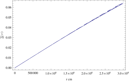
Figure 1: Variation of $\Sigma(r)=\sqrt{-g}$, for the BEC string space-time, for different values of $U_{0}$: $U_{0}=10^{6}\;\mathrm{cm^{5}/g\;s^{2}}$ (solid curve), $U_{0}=10^{6.04}\;\mathrm{cm^{5}/g\;s^{2}}$ (dotted curve), $U_{0}=10^{6.08}\;\mathrm{cm^{5}/g\;s^{2}}$ (short dashed curve), $U_{0}=10^{6.12}\;\mathrm{cm^{5}/g\;s^{2}}$ (dashed curve), and $U_{0}=10^{6.16}\;\mathrm{cm^{5}/g\;s^{2}}$ (long dashed curve), respectively.

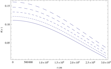
Figure 2: Variation of the dimensionless density $\theta(r)=U_{0}\rho(r)/c^{2}$ of the BEC string, for different values of $U_{0}$: $U_{0}=10^{6}\;\mathrm{cm^{5}/g\;s^{2}}$ (solid curve), $U_{0}=10^{6.04}\;\mathrm{cm^{5}/g\;s^{2}}$ (dotted curve), $U_{0}=10^{6.08}\;\mathrm{cm^{5}/g\;s^{2}}$ (short dashed curve), $U_{0}=10^{6.12}\;\mathrm{cm^{5}/g\;s^{2}}$ (dashed curve), and $U_{0}=10^{6.16}\;\mathrm{cm^{5}/g\;s^{2}}$ (long dashed curve), respectively.

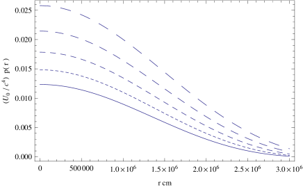
Figure 3: Variation of the dimensionless pressure $\theta^{2}(r)=\left(U_{0}/c^{4}\right)p(r)$ of the BEC string, for different values of $U_{0}$: $U_{0}=10^{6}\;\mathrm{cm^{5}/g\;s^{2}}$ (solid curve), $U_{0}=10^{6.04}\;\mathrm{cm^{5}/g\;s^{2}}$ (dotted curve), $U_{0}=10^{6.08}\;\mathrm{cm^{5}/g\;s^{2}}$ (short dashed curve), $U_{0}=10^{6.12}\;\mathrm{cm^{5}/g\;s^{2}}$ (dashed curve), and $U_{0}=10^{6.16}\;\mathrm{cm^{5}/g\;s^{2}}$ (long dashed curve), respectively.

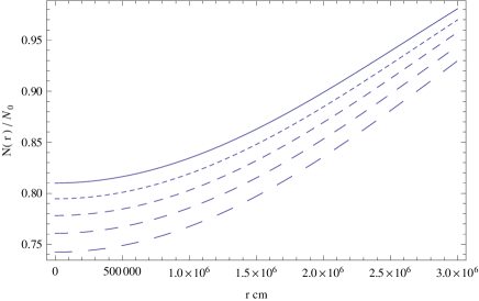
Figure 4: Variation of the function $N(r)/N_{0}\propto\sqrt{g_{tt}}$, for the BEC string space-time, for different values of $U_{0}$: $U_{0}=10^{6}\;\mathrm{cm^{5}/g\;s^{2}}$ (solid curve), $U_{0}=10^{6.04}\;\mathrm{cm^{5}/g\;s^{2}}$ (dotted curve), $U_{0}=10^{6.08}\;\mathrm{cm^{5}/g\;s^{2}}$ (short dashed curve), $U_{0}=10^{6.12}\;\mathrm{cm^{5}/g\;s^{2}}$ (dashed curve), and $U_{0}=10^{6.16}\;\mathrm{cm^{5}/g\;s^{2}}$ (long dashed curve), respectively.

Figure 5: Variation of $L(r)=\sqrt{-g_{\phi\phi}}$, for the BEC string space-time, for different values of $U_{0}$: $U_{0}=10^{6}\;\mathrm{cm^{5}/g\;s^{2}}$ (solid curve), $U_{0}=10^{6.04}\;\mathrm{cm^{5}/g\;s^{2}}$ (dotted curve), $U_{0}=10^{6.08}\;\mathrm{cm^{5}/g\;s^{2}}$ (short dashed curve), $U_{0}=10^{6.12}\;\mathrm{cm^{5}/g\;s^{2}}$ (dashed curve), and $U_{0}=10^{6.16}\;\mathrm{cm^{5}/g\;s^{2}}$ (long dashed curve), respectively.

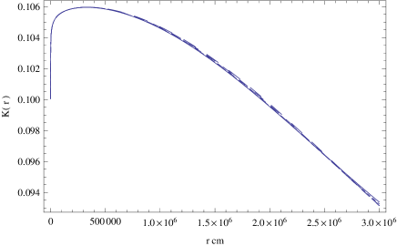
Figure 6: Variation of $K(r)=\sqrt{-g_{zz}}$, for the BEC string space-time, for different values of $U_{0}$: $U_{0}=10^{6}\;\mathrm{cm^{5}/g\;s^{2}}$ (solid curve), $U_{0}=10^{6.04}\;\mathrm{cm^{5}/g\;s^{2}}$ (dotted curve), $U_{0}=10^{6.08}\;\mathrm{cm^{5}/g\;s^{2}}$ (short dashed curve), $U_{0}=10^{6.12}\;\mathrm{cm^{5}/g\;s^{2}}$ (dashed curve), and $U_{0}=10^{6.16}\;\mathrm{cm^{5}/g\;s^{2}}$ (long dashed curve), respectively.

Figure 7: Variation of the Tolman mass $M(r)$ of the BEC string, for different values of $U_{0}$: $U_{0}=10^{6}\;\mathrm{cm^{5}/g\;s^{2}}$ (solid curve), $U_{0}=10^{6.04}\;\mathrm{cm^{5}/g\;s^{2}}$ (dotted curve), $U_{0}=10^{6.08}\;\mathrm{cm^{5}/g\;s^{2}}$ (short dashed curve), $U_{0}=10^{6.12}\;\mathrm{cm^{5}/g\;s^{2}}$ (dashed curve), and $U_{0}=10^{6.16}\;\mathrm{cm^{5}/g\;s^{2}}$ (long dashed curve), respectively.

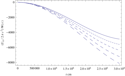
Figure 8: Variation of the angular deficit parameter $W(r)$ of the BEC string, for different values of $U_{0}$: $U_{0}=10^{6}\;\mathrm{cm^{5}/g\;s^{2}}$ (solid curve), $U_{0}=10^{6.04}\;\mathrm{cm^{5}/g\;s^{2}}$ (dotted curve), $U_{0}=10^{6.08}\;\mathrm{cm^{5}/g\;s^{2}}$ (short dashed curve), $U_{0}=10^{6.12}\;\mathrm{cm^{5}/g\;s^{2}}$ (dashed curve), and $U_{0}=10^{6.16}\;\mathrm{cm^{5}/g\;s^{2}}$ (long dashed curve), respectively.

As one can see from Fig. 1, for small $r$, the function $\Sigma(r)=\sqrt{-g}$ appears to be (approximately) proportional to $r$, but with constant of proportionality much less than one (compared to $\Sigma(r)=\sqrt{-g}=r$ for a flat conical geometry, such as that obtained for a vacuum string). The dimensionless density $\theta(r)=U_{0}\rho(r)/c^{2}$, presented in Fig. 2, appears, roughly, to be a Bell-shaped curve. It monotonically decreases from a maximum central value at $r=0$ (as expected intuitively), and reaches the value $\theta=0$ at some finite value of $r$, which defines the radius of the string $R_{s}$, $\theta\left(R_{s}\right)=0$. In the examples considered, the radius of the string is of the order of $R_{s}\approx 3\times 10^{6}\;\mathrm{cm}\approx 30\;\mathrm{km}$. The physical pressure, $p(r)\propto\theta^{2}(r)$, of the Bose-Einstein condensate that forms the string interior, which is shown in Fig. 3, also becomes zero for $r=R_{s}$, that is, at the vacuum boundary of the string. The behavior of the functions that determine the metric tensor components, depicted in Figs. 4-6, show very different variation with respect to the radial coordinate: $N(r)/N_{0}\propto\sqrt{g_{tt}}$ is a monotonically increasing function of $r$, and is roughly proportional to $r$ at large radii. For small $r$, $L(r)=\sqrt{-g_{\phi\phi}}$ is also roughly proportional to $r$, but with a constant of proportionality much less than one. For large $r$, $L(r)$ varies according to some power of $r$, $r^{\delta}$, where $0<\delta<1$. This is in sharp contrast with the flat conical geometry of a vacuum string, for which $L(r)=\sqrt{-g_{\phi\phi}}=r$. The metric function $K(r)=\sqrt{-g_{zz}}$ rises sharply from its initial value, and peaks rapidly, before decreasing monotonically. This behavior is again very different, as compared to $K(r)=\sqrt{-g_{zz}}=1$, which corresponds to flat conical Minkowski space. The Tolman mass function, presented in Fig. 7, is monotonically increasing, and reaches its maximum value at $r=R_{s}$, giving a total mass per unit length for the BEC string (in the examples considered) of the order $M\approx 4-6\times 10^{3}\times\left(2\pi c^{2}\right)/U_{0}\approx 2-3\times 10^{19}$ g. This is extremely small (for reasonable values of $U_{0}$), compared to the masses of possible BEC matter neutron stars, for example, which are of the order of $M\approx 2.8\times 10^{33}$ g. The angular deficit parameter $W(r)$, plotted in Fig. 8, has negative values inside the string, and monotonically decreases as it approaches the string boundary.

This latter observation is perhaps the most intriguing aspect of the BEC string as it allows, in principle, for an “angle excess” in the resulting space-time, according to Eqs. (40)-(42). The term angle excess is used to describe conical geometries in which the deficit angle exceeds $2\pi$. Though these may be considered unphysical, Visser has suggested that, instead, such configurations correspond to negative mass strings (composed of exotic matter), which may be capable of supporting a traversable wormhole Visser1989 . An example of such an exotic string, originally proposed in WormholeStrings1 , is one with vanishing radial and azimuthal stresses ($T_{r}=T_{\phi}=0,\ \forall r$), for which the mass per unit length $\mu$ is equal to the longitudinal tension $T_{z}$, both of which are negative, i.e. $\mu=T_{z}<0$, and further work has since been carried out in relation to this idea WormholeStrings2 . The exoticness of such an object may be judged against the corresponding condition for Nambu-Goto or vacuum string, $\mu=-T_{z}>0$. Since the BEC string, considered here, clearly has positive mass and positive pressure (i.e. negative tension) in the longitudinal direction, this raises the intriguing question as to whether exotic negative mass objects are really required to support traversable wormholes, or whether other cylindrically symmetric mass distributions, obeying reasonable sets of energy conditions (for example, the trace energy condition Eq. (33)), may be able to behave exotically, given the right initial conditions.

III.4 Quantum pressure dominated Bose-Einstein condensate strings

In this section we assume that the BEC string is supported by its quantum pressure $p_{Q}$, given by Eq. (14), which satisfies the condition $p_{Q}>>p=U_{0}\rho^{2}$. By adopting the Newtonian approximation for the quantum regime, and assuming that the gravitational field does not affect the fundamental quantum properties of the system, as formulated in the standard Hilbert space approach, the three-dimensional Laplacian operator, $\vec{\nabla}^{2}$, for cylindrically symmetry systems, is given by

$$\Delta=\frac{1}{r}\frac{d}{dr}\left(r\frac{d}{dr}\right).$$ (68)

Therefore, the gravitational field equations describing the quantum pressure supported BEC string take the form

$$\frac{1}{\Sigma}\frac{d}{dr}\left(\Sigma H_{t}\right)=\frac{4\pi G}{c^{2}}\rho\left[1-3\frac{\hbar^{2}}{4m^{2}c^{2}}\frac{1}{r}\frac{d}{dr}\left(r\frac{d}{dr}\ln\frac{\rho}{\rho_{c}}\right)\right],$$ (69)

$$3\frac{dH}{dr}+H_{t}^{2}+H_{\phi}^{2}+H_{z}^{2}=$$

$$-\frac{4\pi G}{c^{2}}\rho\left[1+\frac{\hbar^{2}}{4m^{2}c^{2}}\frac{1}{r}\frac{d}{dr}\left(r\frac{d}{dr}\ln\frac{\rho}{\rho_{c}}\right)\right],$$ (70)

$$\frac{1}{\Sigma}\frac{d}{dr}\left(\Sigma H_{i}\right) = -\frac{4\pi G}{c^{2}}\rho\left[1+\frac{\hbar^{2}}{4m^{2}c^{2}}\frac{1}{r}\frac{d}{dr}\left(r\frac{d}{dr}\ln\frac{\rho}{\rho_{c}}\right)\right],$$ (71)

$$i=\phi,z,$$

where $\rho_{c}$ is the central density of the string. The corresponding Tolman mass is given by

$$M(r)=2\pi\int_{0}^{r}{\rho\left[1+3\frac{\hbar}{4m^{2}c^{2}}\frac{1}{r}\frac{d}{dr}\left(r\frac{d}{dr}\ln\frac{\rho}{\rho_{c}}\right)\right]\Sigma dr}.$$ (72)

As in the case of the interaction energy dominated BEC string, the relation between $H_{\phi}$ and $H_{z}$ is again given by Eq. (48). By introducing the dimensionless variables $\zeta$ and $\tau$, defined as

$$r=\frac{\hbar}{2mc}\zeta,\ \tau=\frac{\rho}{\rho_{c}},$$ (73)

and by denoting

$$\lambda_{Q}=\frac{\pi G\hbar^{2}}{m^{2}c^{4}}\rho_{c},$$ (74)

the field equations describing the quantum pressure dominated BEC string take the following dimensionless form:

$$\frac{1}{\Sigma}\frac{d}{d\zeta}\left(\Sigma{\mathcal{H}}_{t}\right)=\lambda_{Q}\tau\left[1-3\frac{1}{\zeta}\frac{d}{d\zeta}\left(\zeta\frac{d}{d\zeta}\ln\tau\right)\right],$$ (75)

$$3\frac{d{\mathcal{H}}}{d\zeta}+{\mathcal{H}}_{t}^{2}+{\mathcal{H}}_{\phi}^{2}+{\mathcal{H}}_{z}^{2}=-\lambda_{Q}\tau\left[1+\frac{1}{\zeta}\frac{d}{d\zeta}\left(\zeta\frac{d}{d\zeta}\ln\tau\right)\right],$$

$$\frac{1}{\Sigma}\frac{d}{d\zeta}\left(\Sigma{\mathcal{H}}_{i}\right)=-\lambda_{Q}\tau\left[1+\frac{1}{\zeta}\frac{d}{d\zeta}\left(\zeta\frac{d}{d\zeta}\ln\tau\right)\right],i=\phi,z,$$ (77)

where the ${\mathcal{H}}_{\nu}$, $\nu\in\left\{t,\phi,z\right\}$ and ${\mathcal{H}}$ are now defined in terms of the derivatives with respect to $\zeta$, i.e. $\mathcal{H}_{\nu}=(\hbar/2mc)H_{\nu}$, so that $\mathcal{H}_{t}=(1/N)\left(dN/d\zeta\right)$ etc.

The energy conservation equation for the quantum pressure becomes

$$\frac{d}{d\zeta}\left[\tau\frac{1}{\zeta}\frac{d}{d\zeta}\left(\zeta\frac{d}{d\zeta}\ln\tau\right)\right]=\tau\left[1-\frac{1}{\zeta}\frac{d}{d\zeta}\left(\zeta\frac{d}{d\zeta}\ln\tau\right)\right]{\mathcal{H}}_{t},$$ (78)

and its dimensionless equivalent, $P_{Q}=p_{Q}/\rho_{c}c^{2}$, may be written as

$$P_{Q}=-\tau\frac{1}{\zeta}\frac{d}{d\zeta}\left(\zeta\frac{d}{d\zeta}\ln\tau\right).$$ (79)

By adding Eqs. (75) and (77) we obtain

$$\frac{1}{\Sigma}\frac{d^{2}\Sigma}{d\zeta^{2}}=-\lambda_{Q}\tau\left[1+5\frac{1}{\zeta}\frac{d}{d\zeta}\left(\zeta\frac{d}{d\zeta}\ln\tau\right)\right],$$ (80)

while Eqs. (75) and (77) for ${\mathcal{H}}_{z}$ can be written as

$$\frac{d{\mathcal{H}}_{t}}{d\zeta}+\frac{1}{\Sigma}\frac{d\Sigma}{d\zeta}{\mathcal{H}}_{t}=\lambda_{Q}\tau\left[1-3\frac{1}{\zeta}\frac{d}{d\zeta}\left(\zeta\frac{d}{d\zeta}\ln\tau\right)\right],$$ (81)

and

$$\frac{d{\mathcal{H}}_{z}}{d\zeta}+\frac{1}{\Sigma}\frac{d\Sigma}{d\zeta}{\mathcal{H}}_{z}=-\lambda_{Q}\tau\left[1+\frac{1}{\zeta}\frac{d}{d\zeta}\left(\zeta\frac{d}{d\zeta}\ln\tau\right)\right],$$ (82)

respectively. Equivalently, the system of field equations obtained above, which may be viewed as a relativistic generalization of the cylindrical Lane-Emden equation discussed in Sect. II.2, can then be formulated as a system of first-order differential equations, i.e.

$$\frac{d\tau}{d\zeta}=a,\frac{d\Sigma}{d\zeta}=\sigma,\frac{dN}{d\zeta}=n,\frac{dK}{d\zeta}=k,$$ (83)

$$\frac{da}{d\zeta}=\tau u+\frac{a^{2}}{\tau}-\frac{a}{\zeta},$$ (84)

$$\frac{du}{d\zeta}=(1-u)\frac{n}{N}-\frac{au}{\tau},$$ (85)

$$\frac{dv}{d\zeta}=-\lambda_{Q}\tau(1+5u)\Sigma,$$ (86)

$$\frac{dn}{d\zeta}=\lambda_{Q}\tau(1-3u)N+\frac{n^{2}}{N}-\frac{\sigma}{\Sigma}n,$$ (87)

$$\frac{dk}{d\zeta}=-\lambda_{Q}\theta(1+u)K+\frac{k^{2}}{K}-\frac{\sigma}{\Sigma}{k},$$ (88)

which must be integrated subject to the initial conditions $\tau(0)=1$, $a(0)=\tau^{\prime}(0)=\tau_{0}^{\prime}$, $u(u)=u_{0}^{\prime}$, $N(0)=1$, $n(0)=N^{\prime}(0)=0$, $K(0)=K_{0}$, $k(0)=K^{\prime}(0)=K_{0}^{\prime}$, $\Sigma(0)=\Sigma_{0}$ and $\sigma(0)=\Sigma^{\prime}(0)=\sigma_{0}^{\prime}$, where a prime now indicates differentiation with respect to $\zeta$. The dimensionless form of the Tolman mass, $m(\zeta)=M(\zeta)/\left(\pi\hbar^{2}\rho_{c}/2m^{2}c^{2}\right)$, is given by

$$m(\zeta) = 2\pi\int_{\zeta^{\prime}=0}^{\zeta}\tau\left(\zeta^{\prime}\right)\left[1+3\frac{1}{\zeta^{\prime}}\frac{d}{d\zeta^{\prime}}\left(\zeta^{\prime}\frac{d}{d\zeta^{\prime}}\ln\tau\left(\zeta^{\prime}\right)\right)\right]\times$$ (89)

$$\Sigma\left(\zeta^{\prime}\right)d\zeta^{\prime},$$

while the dimensionless angular deficit $w(\zeta)=W(\zeta)/\left(\pi\hbar^{2}\rho_{c}/2m^{2}c^{2}\right)$ is obtained as

$$w(\zeta) = -2\pi\int_{\zeta^{\prime}=0}^{\zeta}\tau\left(\zeta^{\prime}\right)\left[1+\frac{1}{\zeta^{\prime}}\frac{d}{d\zeta^{\prime}}\left(\zeta^{\prime}\frac{d}{d\zeta^{\prime}}\ln\tau\left(\zeta^{\prime}\right)\right)\right]\times$$ (90)

$$\Sigma\left(\zeta^{\prime}\right)d\zeta^{\prime}.$$

The variation, with respect to $\zeta$, of $\Sigma=\sqrt{-g}$, of the dimensionless energy density of the BEC matter $\tau$, the dimensionless quantum pressure $p_{Q}$, the functions $N$, $L$ and $K$ that determine the components of the metric tensor, the dimensionless Tolman mass $m$, and the angular deficit parameter $w$ are represented, for different values of the parameter $\lambda_{Q}$, in Figs. 9-16. In each case, the initial conditions used to numerically integrate the system of differential equations, Eqs. (83)–(88), were $\Sigma(0)=0.01$, $\sigma(0)=0.10$, $\tau(0)=1$, $a(0)=0$, $N(0)=1$, $n(0)=-10^{-8}$, $u(0)=-1$, $K(0)=0.01$, $k(0)=-0.01$, $m(0)=0$ and $w(0)=0$.

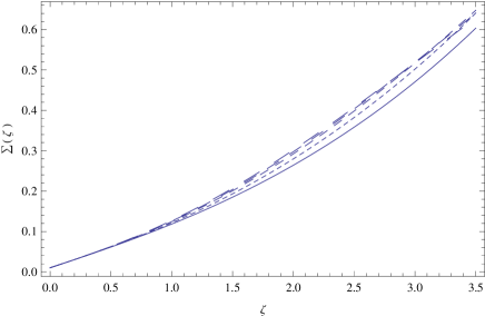
Figure 9: Variation of $\Sigma=\sqrt{-g}$, as a function of $\zeta$, in the space-time of the quantum pressure supported Bose Einstein condensate string, for different values of $\lambda_{Q}$: $\lambda_{Q}=0.10$ (solid curve), $\lambda_{Q}=0.14$ (dotted curve), $\lambda_{Q}=0.18$ (short dashed curve), $\lambda_{Q}=0.20$ (dashed curve), and $\lambda_{Q}=0.22$ (long dashed curve), respectively.

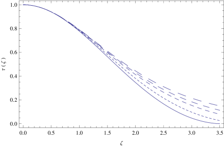
Figure 10: Variation of the dimensionless density $\tau$, as a function of $\zeta$, of the quantum pressure dominated Bose-Einstein condensate string, for different values of $\lambda_{Q}$: $\lambda_{Q}=0.10$ (solid curve), $\lambda_{Q}=0.14$ (dotted curve), $\lambda_{Q}=0.18$ (short dashed curve), $\lambda_{Q}=0.20$ (dashed curve), and $\lambda_{Q}=0.22$ (long dashed curve), respectively.

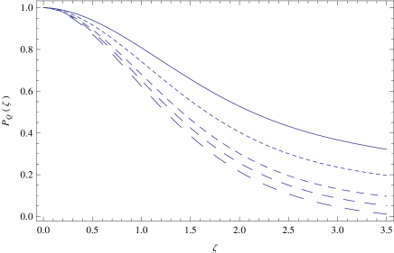
Figure 11: Variation of the dimensionless quantum pressure $P_{Q}$, as a function of $\zeta$, of the quantum pressure dominated Bose-Einstein condensate string, for different values of $\lambda_{Q}$: $\lambda_{Q}=0.10$ (solid curve), $\lambda_{Q}=0.14$ (dotted curve), $\lambda_{Q}=0.18$ (short dashed curve), $\lambda_{Q}=0.20$ (dashed curve), and $\lambda_{Q}=0.22$ (long dashed curve), respectively.

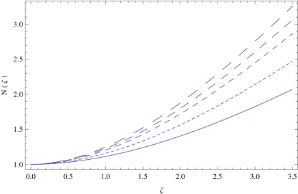
Figure 12: Variation of the $N(\zeta)=\sqrt{g_{tt}}$ for the space-time of the quantum pressure dominated Bose-Einstein condensate string, for different values of $\lambda_{Q}$: $\lambda_{Q}=0.10$ (solid curve), $\lambda_{Q}=0.14$ (dotted curve), $\lambda_{Q}=0.18$ (short dashed curve), $\lambda_{Q}=0.20$ (dashed curve), and $\lambda_{Q}=0.22$ (long dashed curve), respectively.

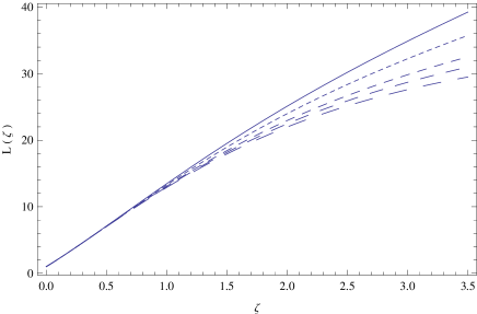
Figure 13: Variation of $L(\zeta)=\sqrt{-g_{\phi\phi}}$ for the space-time of the quantum pressure dominated Bose-Einstein condensate string, for different values of $\lambda_{Q}$: $\lambda_{Q}=0.10$ (solid curve), $\lambda_{Q}=0.14$ (dotted curve), $\lambda_{Q}=0.18$ (short dashed curve), $\lambda_{Q}=0.20$ (dashed curve), and $\lambda_{Q}=0.22$ (long dashed curve), respectively.

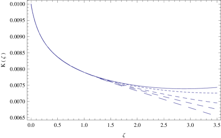
Figure 14: Variation of $K(\zeta)=\sqrt{-g_{zz}}$ for the space-time of the quantum pressure dominated Bose-Einstein condensate string, for different values of $\lambda_{Q}$: $\lambda_{Q}=0.10$ (solid curve), $\lambda_{Q}=0.14$ (dotted curve), $\lambda_{Q}=0.18$ (short dashed curve), $\lambda_{Q}=0.20$ (dashed curve), and $\lambda_{Q}=0.22$ (long dashed curve), respectively.

Figure 15: Variation of the Tolman mass $m$, as a function of $\zeta$, of the quantum pressure dominated Bose-Einstein condensate string, for different values of $\lambda_{Q}$: $\lambda_{Q}=0.10$ (solid curve), $\lambda_{Q}=0.14$ (dotted curve), $\lambda_{Q}=0.18$ (short dashed curve), $\lambda_{Q}=0.20$ (dashed curve), and $\lambda_{Q}=0.22$ (long dashed curve), respectively.

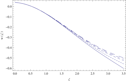
Figure 16: Variation of the angular deficit $w$, as a function of $\zeta$, of the quantum pressure dominated Bose-Einstein condensate string, for different values of $\lambda_{Q}$: $\lambda_{Q}=0.10$ (solid curve), $\lambda_{Q}=0.14$ (dotted curve), $\lambda_{Q}=0.18$ (short dashed curve), $\lambda_{Q}=0.20$ (dashed curve), and $\lambda_{Q}=0.22$ (long dashed curve), respectively.

The variation of the function $\Sigma(\zeta)=\sqrt{-g}$, presented in Fig 9, appears to be approximately proportional to $\zeta$, for small $\zeta$, but varies according to a higher power of $\zeta$ as $\zeta$ increases. This is in contrast to the interaction pressure dominated case, as well to the $\Sigma=\sqrt{-g}\propto\zeta$ case for a flat conical geometry. The dimensionless density $\tau(\zeta)=\rho(\zeta)/\rho_{c}(\zeta)$ of the BEC cosmic string, plotted in Fig. 10, monotonically decreases from a maximum central value at $\zeta=0$, reaching the value zero for $\zeta=\zeta_{s}$, which defines the vacuum boundary of the string.

For the parameters used in the numerical simulations it follows that $R_{s}\approx 3.5\hbar/2mc=6.148\times 10^{-38}/m$. If the mass of the particle in the condensate is very small, $m\approx 10^{-44}$ g, then $R_{s}\approx 6.16\times 10^{6}$ cm. On the other hand, more massive particles can form condensate strings with very small radii. At the vacuum boundary $\zeta=\zeta_{s}$ the quantum pressure, depicted in Fig. 11, tends to zero, together with the energy density of the BEC particles. However, its relationship with the energy density is now more complex than in the interaction pressure dominated case. $N(\zeta)/N_{0}\propto\sqrt{g_{tt}}$, presented in Fig. 12, is a monotonically increasing function of $\zeta$ and it becomes proportional to $\zeta$ at large radial distances. Its behavior is qualitatively similar to that found in the space-time of the interaction pressure dominated string. Likewise, $L(\zeta)=\sqrt{-g_{\phi\phi}}$, shown in Fig. 13, behaves in much the same way as for the interaction pressure dominated string. The major difference in the behavior of the metric components, between the interaction and quantum pressure dominated regimes, comes from $K=\sqrt{-g_{zz}}$, represented in Fig. 14. In the latter, $K(\zeta)$ decreases monotonically as a function of the radial distance, with a sharp immediate drop close to $\zeta=0$, followed by a more gradual decline. Again, the Tolman mass function, plotted in Fig. 15, is monotonically increasing and tends to a constant value $M\approx 0.8-1.4\times\left(\pi\hbar^{2}/2m^{2}c^{2}\right)\rho_{c}\approx 2.71\times 10^{-75}\left(\rho_{c}/m^{2}\right)$, giving the total mass of the quantum BEC string. For an ultralight particle with $m=10^{-44}$ g we obtain $M\approx 2.71\times 10^{13}\rho_{c}$. Particles with such masses may be the axions of quantum chromodynamics, pseudo Nambu-Goldstone bosons associated with the spontaneous breaking of Peccei-Quinn symmetry, which represent an important dark matter candidate axion . Such axions are also believed to form nonstring BECs Sikivie:2009qn and, while astrophysical constraints on axionlike dark matter candidates can be obtained from big bang nucleosynthesis data, a number of direct detection schemes have recently been proposed, based on their predicted interactions with solid state and atomic systems Budker:2013hfa ; Roberts:2014dda . By using the most recent cosmological data, including the Planck temperature data, the WMAP E-polarization measurements, the recent BICEP2 observations of B-modes, as well as baryon acoustic oscillation data, including those from the Baryon Oscillation Spectroscopic Survey Valent , it was found that the mass of dark matter axions is constrained to lie in the range of $70-80$ $\mu\mathrm{eV}$. Lighter dark matter particles are also possible.

Thus, if the central density is sufficiently high, quantum strings may have masses of the order of $M\approx 10^{-7}M_{\odot}$. The angular deficit $w$, shown in Fig. 16, is again negative inside the string, and it is a monotonically decreasing function of the radial distance. This suggests that the possibility of BEC strings giving rise to space-time angle excess cannot be excluded in either the $p\gg P_{Q}$ or $p\ll P_{Q}$ regimes and, hence, that it may, in principle, be a generic feature of such strings, given appropriate initial conditions. However, further investigation is required in order to determine just how generic these conditions may be, and whether or not they are comparable in each regime.

III.5 Quantum pressure dominated Bose-Einstein condensate strings: the effects of the gravitational field on the equation of state

In the previous section, we considered the properties of quantum pressure dominated Bose-Einstein condensate strings by assuming that the equation of state of the string is independent of the background gravitational field. From a mathematical point of view, this means we have assumed that the Laplacian operator $\vec{\nabla}^{2}$, acting on the density, can be defined in the standard Euclidian space of quantum mechanics. Hence, in this approach, the local quantum equation of state is not affected by the curvature of the space-time (the gravitational field), an approximation which is consistent with the semiclassical limit of general relativity. However, since the quantum equation of state also contains a geometric component (via the presence of the geometry-dependent Laplacian), in the presence of strong gravitational fields, the geometry of the space-time may play a significant role in the physical description of the quantum pressure. Therefore, in this section, we consider the effects of the gravitational field on the quantum pressure equation of state. In order to obtain the equation of state in a curved space-time, we introduce the corresponding three-dimensional Laplacian as

$$\vec{\nabla}^{2}=\frac{1}{L(r)K(r)}\frac{d}{dr}\left[L(r)K(r)\frac{d}{dr}\right],$$ (91)

which allows us to define the quantum pressure as

$$p_{Q}(r)=-\frac{\hbar^{2}}{4m^{2}}\rho(r)\frac{1}{L(r)K(r)}\frac{d}{dr}\left[L(r)K(r)\frac{d}{dr}\ln\frac{\rho(r)}{\rho_{c}}\right].$$ (92)

Hence, by taking into account the gravitational effects on the quantum equation of state, the field equations describing the quantum pressure supported BEC string take the form

$$\frac{1}{\Sigma}\frac{d}{dr}\left(\Sigma H_{t}\right)=\frac{4\pi G}{c^{2}}\rho\left[1-3\frac{\hbar^{2}}{4m^{2}c^{2}}\frac{1}{LK}\frac{d}{dr}\left(LK\frac{d}{dr}\ln\frac{\rho}{\rho_{c}}\right)\right],$$ (93)

$$3\frac{dH}{dr}+H_{t}^{2}+H_{\phi}^{2}+H_{z}^{2}=$$

$$-\frac{4\pi G}{c^{2}}\rho\left[1+\frac{\hbar^{2}}{4m^{2}c^{2}}\frac{1}{LK}\frac{d}{dr}\left(LK\frac{d}{dr}\ln\frac{\rho}{\rho_{c}}\right)\right],$$ (94)

$$\frac{1}{\Sigma}\frac{d}{dr}\left(\Sigma H_{i}\right) = -\frac{4\pi G}{c^{2}}\rho\left[1+\frac{\hbar^{2}}{4m^{2}c^{2}}\frac{1}{LK}\frac{d}{dr}\left(LK\frac{d}{dr}\ln\frac{\rho}{\rho_{c}}\right)\right],$$ (95)

$$i=\phi,z,$$

where $\rho_{c}$ is again the central density of the string. The corresponding Tolman mass is given by

$$M(r) = 2\pi\int_{r^{\prime}=0}^{r}\rho\left(r^{\prime}\right)\Bigg{\{}1+3\frac{\hbar}{4m^{2}c^{2}}\frac{1}{L\left(r^{\prime}\right)K\left(r^{\prime}\right)}\times$$

$$\frac{d}{dr^{\prime}}\left[L\left(r^{\prime}\right)K\left(r^{\prime}\right)\frac{d}{dr^{\prime}}\ln\frac{\rho\left(r^{\prime}\right)}{\rho_{c}}\right]\Bigg{\}}\Sigma\left(r^{\prime}\right)dr^{\prime},$$

while

$$W(r)=-2\pi\int_{r^{\prime}=0}^{r}\rho\left(r^{\prime}\right)\Bigg{\{}1+\frac{\hbar}{4m^{2}c^{2}}\frac{1}{L\left(r^{\prime}\right)K\left(r^{\prime}\right)}\times$$

$$\frac{d}{dr^{\prime}}\left[L\left(r^{\prime}\right)K\left(r^{\prime}\right)\frac{d}{dr^{\prime}}\ln\frac{\rho\left(r^{\prime}\right)}{\rho_{c}}\right]\Bigg{\}}\Sigma\left(r^{\prime}\right)dr^{\prime}.$$ (97)

The relation between $H_{\phi}$ and $H_{z}$ is again obtained as $H_{\phi}=H_{z}+C/\Sigma$. By introducing the same set of dimensionless quantities as in the previous section, we obtain the basic equations of the new model in a dimensionless form:

$$\frac{1}{\Sigma}\frac{d^{2}\Sigma}{d\zeta^{2}}=-\lambda_{Q}\tau\left[1+5\frac{1}{LK}\frac{d}{d\zeta}\left(LK\frac{d}{d\zeta}\ln\tau\right)\right],$$ (98)

$$\frac{d}{d\zeta}\left[\tau\frac{1}{LK}\frac{d}{d\zeta}\left(LK\frac{d}{d\zeta}\ln\tau\right)\right]-\tau\Bigg{[}1-$$

$$\frac{1}{LK}\frac{d}{d\zeta}\left(LK\frac{d}{d\zeta}\ln\tau\right)\Bigg{]}{\mathcal{H}}_{t}=0,$$ (99)

$$\frac{d{\mathcal{H}}_{t}}{d\zeta}+\frac{1}{\Sigma}\frac{d\Sigma}{d\zeta}{\mathcal{H}}_{t}=\lambda_{Q}\tau\left[1-3\frac{1}{LK}\frac{d}{d\zeta}\left(LK\frac{d}{d\zeta}\ln\tau\right)\right],$$ (100)

$$\frac{d{\mathcal{H}}_{\phi}}{d\zeta}+\frac{1}{\Sigma}\frac{d\Sigma}{d\zeta}{\mathcal{H}}_{\phi}=-\lambda_{Q}\tau\left[1+\frac{1}{LK}\frac{d}{d\zeta}\left(LK\frac{d}{d\zeta}\ln\tau\right)\right],$$ (101)

$$\frac{d{\mathcal{H}}_{z}}{d\zeta}+\frac{1}{\Sigma}\frac{d\Sigma}{d\zeta}{\mathcal{H}}_{z}=-\lambda_{Q}\tau\left[1+\frac{1}{LK}\frac{d}{d\zeta}\left(LK\frac{d}{d\zeta}\ln\tau\right)\right],$$ (102)

$$m(\zeta)=2\pi\int_{\zeta^{\prime}=0}^{\zeta}{\tau\left[1+3\frac{1}{LK}\frac{d}{d\zeta^{\prime}}\left(LK\frac{d}{d\zeta^{\prime}}\ln\tau\right)\right]\Sigma d\zeta^{\prime}},$$ (103)

$$w(\zeta)=-2\pi\int_{\zeta^{\prime}=0}^{\zeta}{\tau\left[1+\frac{1}{LK}\frac{d}{d\zeta^{\prime}}\left(LK\frac{d}{d\zeta^{\prime}}\ln\tau\right)\right]\Sigma d\zeta^{\prime}}.$$ (104)

The quantum pressure can be obtained in a dimensionless form as

$$P_{Q}=-\tau\frac{1}{LK}\frac{d}{d\zeta}\left(LK\frac{d}{d\zeta}\ln\tau\right).$$ (105)

In order to numerically integrate the system of Eqs. (98)-(104), we choose the initial conditions identical to those in the previous section. Hence we adopt the initial values for the geometrical and physical parameters on the string axis as $N(0)=1$, $L(0)=0.01$, $K(0)=0.01$, $H_{t}(0)=N^{\prime}(0)/N(0)=-10^{(}-8)$, $H_{\phi}(0)=L^{\prime}(0)/L(0)=100$, $H_{z}(0)=K^{\prime}(0)/K(0)=-1$, $\tau(0)=1$, $\tau^{\prime}(0)=0$, $\tau^{\prime\prime}(0)=-0.0001$, $\Sigma(0)=10^{-8}$, $\Sigma^{\prime}(0)=0.1$, $m(0)=0$ and $w(0)=0$, respectively. Hence we have also adopted identical initial conditions for both $L$ and $K$. The variations, with respect to the dimensionless radial distance $\zeta$, of the square root of the determinant of the metric tensor $\Sigma=NKL$, the individual functions $N$, $L$ and $K$, the dimensionless mass density $\tau$, and the quantum pressure inside the string $P_{Q}$, as well as the Tolman mass and the angular deficit parameter $w$, are presented, for different values of the free parameter $\lambda_{Q}$, in Figs. 17-24.

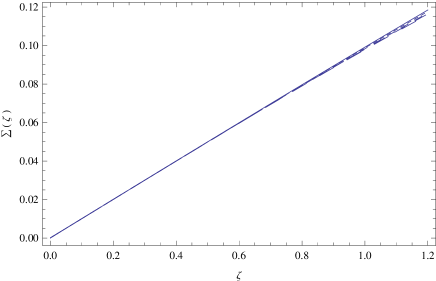
Figure 17: Variation of $\Sigma=\sqrt{-g}$, as a function of $\zeta$, in the space-time of the quantum pressure supported Bose-Einstein condensate string with geometry-dependent equation of state, for different values of $\lambda_{Q}$: $\lambda_{Q}=0.10$ (solid curve), $\lambda_{Q}=0.14$ (dotted curve), $\lambda_{Q}=0.18$ (short dashed curve), $\lambda_{Q}=0.20$ (dashed curve), and $\lambda_{Q}=0.22$ (long dashed curve), respectively.

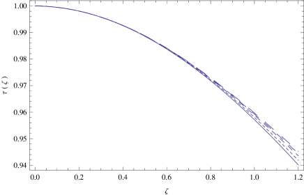
Figure 18: Variation of the dimensionless density $\tau$, as a function of $\zeta$, of the quantum pressure dominated Bose-Einstein condensate string with geometry-dependent equation of state, for different values of $\lambda_{Q}$: $\lambda_{Q}=0.10$ (solid curve), $\lambda_{Q}=0.14$ (dotted curve), $\lambda_{Q}=0.18$ (short dashed curve), $\lambda_{Q}=0.20$ (dashed curve), and $\lambda_{Q}=0.22$ (long dashed curve), respectively.

Figure 19: Variation of the dimensionless quantum pressure $P_{Q}$, as a function of $\zeta$, of the quantum pressure dominated Bose-Einstein condensate string with geometry-dependent equation of state, for different values of $\lambda_{Q}$: $\lambda_{Q}=0.10$ (solid curve), $\lambda_{Q}=0.14$ (dotted curve), $\lambda_{Q}=0.18$ (short dashed curve), $\lambda_{Q}=0.20$ (dashed curve), and $\lambda_{Q}=0.22$ (long dashed curve), respectively.

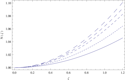
Figure 20: Variation of the $N(\zeta)=\sqrt{g_{tt}}$ for the space-time of the quantum pressure dominated Bose-Einstein condensate string with geometry-dependent equation of state, for different values of $\lambda_{Q}$: $\lambda_{Q}=0.10$ (solid curve), $\lambda_{Q}=0.14$ (dotted curve), $\lambda_{Q}=0.18$ (short dashed curve), $\lambda_{Q}=0.20$ (dashed curve), and $\lambda_{Q}=0.22$ (long dashed curve), respectively.

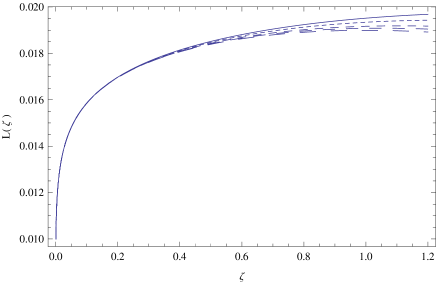
Figure 21: Variation of $L(\zeta)=\sqrt{-g_{\phi\phi}}$ for the space-time of the quantum pressure dominated Bose-Einstein condensate string with geometry-dependent equation of state, for different values of $\lambda_{Q}$: $\lambda_{Q}=0.10$ (solid curve), $\lambda_{Q}=0.14$ (dotted curve), $\lambda_{Q}=0.18$ (short dashed curve), $\lambda_{Q}=0.20$ (dashed curve), and $\lambda_{Q}=0.22$ (long dashed curve), respectively.

Figure 22: Variation of $K(\zeta)=\sqrt{-g_{zz}}$ for the space-time of the quantum pressure dominated Bose-Einstein condensate string with geometry-dependent equation of state, for different values of $\lambda_{Q}$: $\lambda_{Q}=0.10$ (solid curve), $\lambda_{Q}=0.14$ (dotted curve), $\lambda_{Q}=0.18$ (short dashed curve), $\lambda_{Q}=0.20$ (dashed curve), and $\lambda_{Q}=0.22$ (long dashed curve), respectively.

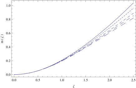
Figure 23: Variation of the Tolman mass $m$, as a function of $\zeta$, of the quantum pressure dominated Bose-Einstein condensate string with geometry-dependent equation of state, for different values of $\lambda_{Q}$: $\lambda_{Q}=0.10$ (solid curve), $\lambda_{Q}=0.14$ (dotted curve), $\lambda_{Q}=0.18$ (short dashed curve), $\lambda_{Q}=0.20$ (dashed curve), and $\lambda_{Q}=0.22$ (long dashed curve), respectively.

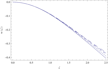
Figure 24: Variation of the angular deficit $w$, as a function of $\zeta$, of the quantum pressure dominated Bose-Einstein condensate string with geometry-dependent equation of state, for different values of $\lambda_{Q}$: $\lambda_{Q}=0.10$ (solid curve), $\lambda_{Q}=0.14$ (dotted curve), $\lambda_{Q}=0.18$ (short dashed curve), $\lambda_{Q}=0.20$ (dashed curve), and $\lambda_{Q}=0.22$ (long dashed curve), respectively.

The behavior of the physical parameters of the Bose-Einstein condensate string, in the presence of a space-time geometry-dependent quantum pressure, is qualitatively similar to the behavior of the same parameters in the case of the “simplified” quantum equation of state, in which the influence of the background geometry is neglected. However, some quantitative differences do arise due to the gravitational influence on the equation of state. As a general result, and for the specific initial values of the geometrical and physical quantities adopted in the examples given above, the string becomes more compact, and its radius as well as its mass decrease slightly, as compared to semiclassical approximation. Again, the square root of the determinant of the metric tensor, shown in Fig. 17, is a monotonically increasing function of the radial distance $\zeta$. For small values of $\zeta$ the increase is linear, and practically independent of the values of the parameter $\lambda_{Q}$. For large values of $\zeta$ the increase can be approximately described by a second degree algebraic function, but the deviations from the linear regime are extremely small. The energy density $\tau$ of the string, represented in Fig. 18, is a monotonically decreasing function of $\zeta$. As usual, the quantum pressure, presented in Fig. 19, monotonically decreases with $\zeta$ and reaches zero at the vacuum boundary of the string, corresponding to $P_{Q}\left(R_{s}\right)=0$. The geometric effects on the equation of state significantly reduce the central values of the quantum pressure, due to the explicit dependence on the metric functions, while increasing the rate at which $P_{Q}$ approaches zero. The value of the radial coordinate $\zeta$ for which the quantum pressure becomes zero can be taken as describing the quantum string radius, which for the adopted values of the parameter $\lambda_{Q}$ is in the range $R_{s}\approx(1.2-2)\times\hbar/2mc=(2.108-3.513)\times 10^{6}\times\left(m/10^{-44}\;{\rm g}\right)^{-1}\;{\rm cm}$. For a particle with mass $m=10^{-44}$ g the Bose-Einstein condensate string radii are of the same order of magnitude as the neutron star radii. This radius is slightly lower than the corresponding radius of the simplified quantum string model, showing that gravitational effects in the quantum pressure indeed make the string more compact.

The metric tensor components $N(\zeta)$ and $L(\zeta)$, represented in Figs. 20 - 21, are increasing functions of $\zeta$, and their behavior is similar to in the simplified quantum pressure case. For small values of $\zeta$, $L(\zeta)$ increases linearly, but sharply, while $N(\zeta)$ is roughly constant. For large values of $\zeta$, near the string vacuum boundary, $N(\zeta)$ has an approximate second-order polynomial behavior, while $L(\zeta)$ has approximately constant values. Similar to the case of the quantum pressure supported string in the semiclassical approximation, the $g_{zz}$ metric tensor component $K(\zeta)$, shown in Fig. 22, is a decreasing function of $\zeta$. For small values of $\zeta$, the behavior of all three metric functions is independent of $\lambda_{Q}$, and can be approximated by a linear function in the radial distance $\zeta$. The Tolman mass $m$, represented in Fig. 23, is a monotonically increasing function, and reaches the value $m\left(\zeta_{s}\right)\approx 0.35-0.40$ at the string surface. The total mass of the string can therefore be estimated as $M\approx(6.786-7.755)\times 10^{12}\times\left(m/10^{-44}\;{\rm g}\right)^{-2}\times\rho_{c}\;{\rm g}$, which is slightly lower, as compared to the mass of the string in the semiclassical model, in which the effect of the geometry on the quantum equation of state is neglected. The angular deficit parameter inside the string $w$ , plotted in Fig. 24, is again negative, with values in the range $w\in(0,-0.4)$, and reaches higher values on the string boundary, as compared to the simplified, geometry-independent case.

IV The Newtonian Approximation

Due to the invariance of the action of the BEC system, Eq. (II.1), under infinitesimal time translations $t\rightarrow t+\delta$ (with $\delta\vec{r}=\delta\psi=\delta\psi^{*}=0$), the nonrelativistic Hamiltonian, and hence the total energy of the condensed particles in the semiclassical approach to quantum BEC strings in general relativity, is conserved. However, in the Newtonian approximation, the total energy $E$ of a gravitationally bound BEC can, in general, be written in the especially simple way, $E=E_{kin}+E_{int}+E_{grav}$, where $E_{kin}$, $E_{int}$ and $E_{grav}$ denote the kinetic, interaction and gravitational energy, respectively. In this final section, we consider an approximate estimate of the energy only, based on the method used in Pet , which assumes the Newtonian limit for the gravitational field. The kinetic energy per particle is of order $\sim(\hbar^{2}/2mR^{2}+\hbar^{2}/2m\Delta^{2})$, where $R$ gives the radial extension and $\Delta$ is the length of the cylinder. Therefore, the approximate expression for the total kinetic energy of the system is given by

$$E_{kin}\approx\frac{\mathcal{N}\hbar^{2}(R^{2}+\Delta^{2})}{2mR^{2}\Delta^{2}}.$$ (106)

The interaction energy is given by $E_{int}\approx(1/2)(\mathcal{N}^{2}/\mathcal{V})u_{0}$, where $\mathcal{V}$ again denotes the volume of the condensate and $\mathcal{N}$ is the total number of particles, while the gravitational potential energy is $E_{grav}\approx-G\mathcal{M}^{2}/R$, where $\mathcal{M}$ is the total mass and, for simplicity, we have neglected the numerical factor in the expression for the gravitational potential energy corresponding to a cylindrically symmetric mass distribution. Therefore, in the Newtonian approximation, and neglecting numerical factors of order unity, the total energy of the condensate is given by

$$E\approx\mathcal{N}\frac{\hbar^{2}(R^{2}+\Delta^{2})}{mR^{2}\Delta^{2}}+\mathcal{N}^{2}\frac{\hbar^{2}l_{s}}{mR^{2}\Delta}-\frac{G\mathcal{M}^{2}}{R},$$ (107)

where we have used the expressions $u_{0}\sim\lambda\sim\hbar^{2}l_{s}/m$ and $\mathcal{V}\sim R^{2}\Delta$. From Eq. (107) we can obtain a rough estimate of the physical parameters of the BEC string in the interaction energy and quantum potential dominated regimes. The quantum kinetic energy is much bigger than the interaction energy when the parameters of the system satisfy the condition

$$\Delta\gg\mathcal{N}l_{s}\left[1+\mathcal{O}\left(\frac{R^{2}}{\Delta}\right)^{2}\right],$$ (108)

for $\Delta\gg R$, or

$$R\gg\mathcal{N}l_{s}\left[1+\mathcal{O}\left(\frac{\Delta^{2}}{R^{2}}\right)^{2}\right],$$ (109)

for $\Delta\ll R$. Both expressions, Eqs. (108)-(109), hold (approximately), in the limiting case, $\Delta\sim R$, for which the result for a spherically symmetric BEC matter distribution is recovered Pet . Assuming the former case, $\Delta\gg R$, which is far more probable for astrophysical BEC strings, the approximate total energy is given by

$$E\approx\mathcal{N}\frac{\hbar^{2}}{mR^{2}}-\frac{G\mathcal{N}^{2}m^{2}}{R}\leq 0,$$ (110)

where we have used $\mathcal{M}\sim m\mathcal{N}$. This, in turn, gives a lower bound for the radius of a quantum pressure dominated BEC string, i.e.

$$R_{quant}\gtrsim\frac{\hbar^{2}}{Gm^{3}\mathcal{N}}.$$ (111)

Equivalently, this may be rewritten as a bound on the (dimensionless) measure of the mass per unit length, which we now label $G\mu_{quant}$, using $\mathcal{M}=\mu_{quant}\Delta$:

$$G\mu_{quant}\gtrsim\frac{\hbar^{2}}{m^{2}R\Delta},$$ (112)

which illustrates the problem, already mentioned in Sec. III.3, with taking the wire approximation for BEC strings. Due to the presence of the quantum pressure term, which becomes significant for narrow strings since only a small number of particles inhabit a thin cross section, the mass per unit length depends sensitively on the product $R\Delta$. Formally, we may consider an infinitely long string of zero width by taking the limits $\Delta\rightarrow\infty$, $R\rightarrow 0$, such that $R\Delta$ remains finite. Realistically, however, we would like to be able to treat open strings and loops as well as, on cosmological scales, strings whose width is limited simply by causality and the finiteness of the horizon. In such cases, the energy density of the string diverges in the wire approximation because the surface tension becomes focused on an area that shrinks to zero. As stated previously, we would therefore expect both finite width corrections MaedaTurok(1988) and effective rigidity terms Anderson et al.(1997) ; Gregory(1988) ; Gregory(1988)* to be important in constructing an effective action for BEC strings. It is interesting to note that, for the quantum pressure dominated BEC, neither the minimum string radius, nor the minimum mass per unit length depends on the scattering length.
By contrast, the interaction energy dominates the internal dynamics of BEC strings when

$$\Delta\ll\mathcal{N}l_{s}\left[1+\mathcal{O}\left(\frac{R^{2}}{\Delta}\right)^{2}\right],$$ (113)

assuming $\Delta\gg R$. This condition is obviously satisfied by cylindrical BEC systems with very large numbers of particle number in relation to their length or, in other words, by thicker strings (for fixed $l_{s}$), though we cannot say a priori whether a string of radius $R$ and length $\Delta$ will be dominated by quantum or interaction pressure. The condition for stability in the latter case is

$$E\approx\mathcal{N}^{2}\frac{\hbar^{2}l_{s}}{mR^{3}}-\frac{Gm^{2}\mathcal{N}^{2}}{R}\leq 0,$$ (114)

which gives the following constraint for the radius, $R_{int}$, of an interaction pressure dominated string,

$$R_{int}\gtrsim\sqrt{\frac{\hbar^{2}l_{s}}{Gm^{3}}}.$$ (115)

Thus, in this regime, we have that

$$\sqrt{\frac{\hbar^{2}l_{s}}{Gm^{3}}}\lesssim R\ll\Delta\ll\mathcal{N}l_{s},$$ (116)

from which it follows that interaction pressure dominated strings, with characteristic minimum radius, form when BEC systems with a sufficient number of particles, i.e.

$$\mathcal{N}\gg\sqrt{\frac{\hbar^{2}}{Gm^{3}l_{s}}},$$ (117)

adopt cylindrically symmetric distributions. The corresponding bound on the string tension is

$$G\mu_{int}\gg\sqrt{\frac{G\hbar^{2}}{ml_{s}\Delta^{2}}}.$$ (118)

Thus, even using the Newtonian approximation, we can obtain rough estimates of the total energy and length scales associated with the BEC string, in both the interaction and quantum pressure dominated regimes.

V Discussions and final remarks

We have considered the possible existence, in a cosmological or astrophysical setting, of static, cylindrically symmetric, general relativistic structures consisting of matter in a Bose-Einstein condensed phase or, in other words, of Bose-Einstein condensate strings. By adopting a semiclassical approach, in which we assume that the quantum dynamics of the condensate remain unaffected by the gravitational field, and that the gravitational field remains classical and independent of quantum effects, we identified two limiting regimes corresponding to thermodynamic (i.e. particle interaction) pressure and quantum pressure dominated strings. For both these limiting cases, we solved the gravitational field equations for the string interior numerically and determined the corresponding variation, with respect to the radial coordinate, of the components of the metric, the three-dimensional energy density and pressure, the Tolman mass per unit length, $M$, and the $W$ parameter which, in conjunction with the initial conditions for the metric components, determines the angular deficit of the cylindrical space-time.
By defining the boundary of the string as the radius at which the energy density and pressure fall to zero, we also obtained estimates for the order of magnitude values of the string width, which depend sensitively on the mass and scattering length of the BEC particles. However, in general, we are able to conclude that interaction pressure dominates for thick strings, while quantum pressure dominates for thin strings in which the ratio of volume to surface area is small. The precise length scale determining the division between the two is determined by the BEC model parameters. In principle, both interaction and quantum pressure dominated strings may vary from tens of kilometers in diameter to widths comparable to more canonical string species.

Though the space-time of the BEC string exhibits many differences from the flat conical space-time surrounding a vacuum string (or even the spherical(-ish) “cap” that regularizes the vacuum string interior), perhaps its most interesting feature is that it allows for the existence of an angle excess: that is, for an angular deficit larger than $2\pi$. Though this may be considered unphysical, a more intriguing possibility is that such a string could behave exotically, in the sense of being able to support a traversable wormhole, as suggested in Visser1989 - WormholeStrings2 .

The solutions we have obtained describe the interior of the Bose-Einstein condensate string. The density and pressure both vanish at the string boundary and therefore, for $r\geq R_{s}$, an exterior vacuum solution of the gravitational field equations describes the physical and geometrical properties of the space-time. Hence, in order to determine the asymptotic form of the metric, the solutions presented in this paper must be matched onto the exterior cylindrically symmetric vacuum metric. In the case of cylindrical symmetry, and by assuming that the exterior gravitational field is described by standard general relativity, this metric is the Kasner metric Verbin - Matt ,

$$ds^{2}=(kr)^{2\mathcal{A}}dt^{2}-dr^{2}-\beta^{2}(kr)^{2(\mathcal{B}-1)}r^{2}d{\phi}^{2}-(kr)^{2\mathcal{C}}dz^{2},$$ (119)

where $k$ determines the length-scale and $\beta$ is a constant, related to the deficit angle of the conical spacetime. The Kasner metric is characterized by two free parameters which, for the unique vacuum solution, satisfy the two Kasner conditions Kasner ; exact-sol ,

$$\mathcal{A}+\mathcal{B}+\mathcal{C}=\mathcal{A}^{2}+\mathcal{B}^{2}+\mathcal{C}^{2}=1.$$ (120)

The continuity of the gravitational potentials across the vacuum boundary of the string also imposes the conditions

$$N\left(R_{s}\right)=\left(kR_{s}\right)^{\mathcal{A}},L\left(R_{s}\right)=\beta\left(kR_{s}\right)^{\mathcal{B}-1}R_{s},$$

$$K\left(R_{s}\right)=\left(kR_{s}\right)^{\mathcal{C}}.$$ (121)

Equations. (120)-(V) represent a system of five algebraic equations for the five unknowns ${\mathcal{A},\mathcal{B},\mathcal{C},k,\beta}$. Thus, a matching of the interior and exterior solutions would uniquely determine the parameters of the Kasner metric as a function of the physical parameters of the Bose-Einstein condensate forming the string. The standard conic cosmic string solution clv ; Verbin ; Verbin1 is characterized by an asymptotic behavior given by a particular form of the Kasner metric (119), with $\mathcal{A}=\mathcal{C}=0$ and $\mathcal{B}=1$. In this case, the metric is evidently locally flat, with the parameter $\beta$ representing a conic angular deficit. The direct matching of the Bose-Einstein condensate interior string solution to the locally flat metric requires $N\left(R_{s}\right)=1$, $K\left(R_{s}\right)=1$ and $L\left(R_{s}\right)=\beta R_{s}$. Due to the initial conditions considered in our numerical analysis of the BEC string model, such a direct matching between the space-time of the massive string interior and a flat exterior geometry is not possible, though this result is consistent with standard results in general relativity exact-sol . On the other hand, as pointed out in Verbin1 , there exists a second interesting Kasner-type solution with $\mathcal{A}=\mathcal{C}=2/3$ , $\mathcal{B}=-1/3$, which represents the so-called Melvin branch. The Melvin magnetic exterior solution can be matched with the interior BEC string solutions considered in this paper. However, such a matching would require the embedding of the BEC string into an external magnetic field.

Finally, we note that one of the major particle candidates for the formation of BEC strings is dark matter particles. When the critical temperature of a cosmological boson gas, which may have existed in the early Universe, became less than the critical temperature, a Bose-Einstein condensation process may have taken place during the early cosmic history. Hence, most of the present day DM may be in the form of a Bose-Einstein condensate. Thus, during the phase transition from normal to condensate dark matter, BEC-type topological defects may have been generated, and condensed dark matter filaments could have been formed. These dark matter filaments may have some properties in common with the BEC string solutions considered in the present paper.

One observational possibility, which may allow us to detect these structures, and to distinguish them from other string-type species, would be through the detection of gravitational lensing events since, due to their exotic nature, the lensing properties of BEC strings may differ substantially from those of standard defect, or even superstring candidates (c.f. topological_defects ; Shlaer:2005ry and references therein). Intriguingly, the possibility of unique, nongravitational lensing phenomena also arises, since some species of non-BEC DM defects are known to lens electromagnetic radiation in a frequency-dependent manner through an alteration of the photon dispersion relation inside the string core, and this lensing is distinct from frequency-independent gravitational lensing Stadnik:2014cea . Further investigation of both the gravitational and nongravitational lensing properties of BEC strings may therefore be extremely fruitful.

On the other hand, strings (i.e. topological defects) were previously considered as possible seeds for structure formation, but this picture has since been overturned in favor of dark matter seeds. As such, BEC DM strings which represent, in some sense, a combination of strings and dark matter, may turn out to be a better solution for large scale structure formation than either nonstringy DM or non-DM strings individually. In particular, galaxy formation from strong primordial inhomogeneities, such as archioles or clouds of primordial black holes concentrated around intermediate mass, or supermassive black holes could provide a specific implementation of Bose-Einstein condensate strings Sakharov:1994id ; Sakharov:1996xg ; Khlopov:1999tm ; Khlopov:1998uj ; Rubin:2001yw ; Khlopov:2002yi ; Khlopov:2004sc ; Khlopov:2004rw ; Khlopov_meeting ; Khlopov:2008qy . In the present paper we have provided some basic theoretical tools that would enable the in depth investigation of the properties of the BEC strings, and of their cosmological implications.

References

- (1) M. H. Anderson, J. R. Ensher, M. R. Matthews, C. E. Wieman, and E. A. Cornell, Science 269, 198 (1995); C. C. Bradley, C. A. Sackett, J. J. Tollett, and R. G. Hulet, Phys. Rev. Lett. 75, 1687 (1995); K. B. Davis, M. O. Mewes, M. R. Andrews, N. J. van Druten, D. S. Durfee, D. M. Kurn, and W. Ketterle, Phys. Rev. Lett. 75, 3969 (1995).
- (2) F. Dalfovo, S. Giorgini, L. P. Pitaevskii, and S. Stringari, Rev. Mod. Phys. 71, 463 (1999).
- (3) E. A. Cornell and C. E. Wieman, Rev. Mod. Phys. 74, 875 (2002); W. Ketterle, Rev. Mod. Phys. 74, 1131 (2002); R. A. Duine and H. T. C. Stoof, Phys. Rep. 396, 115 (2004).
- (4) Q. Chen, J. Stajic, S. Tan and K. Levin, Phys. Rep. 412, 1 (2005).
- (5) L. Pitaevskii and S. Stringari, Bose-Einstein Condensation (Clarendon Press, Oxford, 2003).
- (6) C. J. Pethick and H. Smith, Bose-Einstein Condensation in Dilute Gases (Cambridge University Press, 2008).
- (7) A. Griffin, T. Nikuni, and E. Zaremba, Bose-condensed Gases at Finite Temperatures (Cambridge University Press, 2009).
- (8) S. J. Sin, Phys. Rev. D50, 3650 (1994); S. U. Ji and S. J. Sin, Phys. Rev. D50, 3655 (1994); W. Hu, R. Barkana, and A. Gruzinov, Phys. Rev. Lett. 85, 1158, (2000); J. Goodman, New Astron. 5, 103 (2000); P. J. E. Peebles, Astrophys. J. 534, L127 (2000); A. Arbey, J. Lesgourgues and P. Salati, Phys. Rev. D 68, 023511 (2003).
- (9) E. Castellanos, C. Escamilla-Rivera, A. Mac’as and D. Núñez, J. Cosmol. Astropart. Phys. 11 (2014) 034; A. Suárez, V. Robles and T. Matos, Astrophys. Space Sci. Proc. 38, 9, p. 107 (2013); K. Kirsten and D.J. Toms, Phys. Rev. D 51, 6886 (1995); B.-H. Li, Ph.D. Thesis, University of Texas, 2013.
- (10) C. G. Boehmer and T. Harko, J. Cosmol. Astropart. Phys. 06 (2007) 025.
- (11) J.-W.Lee, Phys. Lett. B 681, 118 (2009); J.-W. Lee and S. Lim, J. Cosmol. Astropart. Phys. 01 (2010) 007; T. Harko, J. Cosmol. Astropart. Phys. 05, (2011) 022; V. H. Robles and T. Matos, Mon. Not. R. Astron. Soc. 422, 282 (2012); M. Dwornik, Z. Keresztes, and L. A. Gergely, in Recent Development in Dark Matter Research, edited by N. Kinjo, A. Nakajima, (Nova Science Publishers, New York, 2014); F. S. Guzman, F. D. Lora-Clavijo, J. J. Gonzalez-Aviles, and F. J. Rivera-Paleo, Phys. Rev. D 89, 063507 (2014); (2013); T. Harko and E. J. M. Madarassy, J. Cosmol. Astropart. Phys. 01 (2012) 020; B. Kain and H. Y. Ling, Phys. Rev. D 82, 064042 (2010); N. T. Zinner, Physics Research International, 734543 (2011); P.-H. Chavanis, Phys. Rev. D 84, 043531 (2011); P.-H. Chavanis and L. Delfini, Phys. Rev. D 84, 043532 (2011); P.-H. Chavanis, Phys. Rev. D 84, 063518 (2011); P.-H. Chavanis, Phys. Rev. E 84, 031101 (2011); T. Rindler-Daller and P. R. Shapiro, Mon. Not. R. Astron. Soc. 422, 135 (2012); T. Rindler-Daller and P. R. Shapiro, Mod. Phys. Lett. A 29, 1430002 (2014); M. O. C. Pires and J. C. C. de Souza, J. Cosmol. Astropart. Phys. 11, 024 (2012); T. Harko, Phys. Rev. D 83, 123515 (2011); T. Harko and G. Mocanu, Phys. Rev. D 85, 084012 (2012); T. Harko, Mon. Not. R. Astron. Soc. 413, 3095 (2011); P.-H. Chavanis, Astron. Astrophys. 537, A 127 (2012); R. C. Freitas and S. V. B. Goncalves, J. Cosmol. Astropart. Phys. 04 (2013) 049; H. Velten and E. Wamba, Phys. Lett. B 709, 1 (2012); E. J. M. Madarassy and V. T. Toth, Comput. Phys. Commun. 184, 1339 (2013); F. S. Guzman, F. D. Lora-Clavijo, J. J. Gonzalez-Aviles, and F. J. Rivera-Paleo, J. Cosmol. Astropart. Phys. 09 (2013) 034; J. C. C. de Souza and M. O. C. Pires, J. Cosmol. Astropart. Phys. 03 (2014) 010; V. T. Toth, arXiv:1402.0600; T. Harko, Phys. Rev. D 89, 084040 (2014); M.-H. Li and Z.-B. Li, Phys. Rev. D 89, 103512 (2014).
- (12) A. Morris, http://www.tcm.phy.cam.ac.uk/ndd21/
- (13) M. G. Alford, K. Rajagopal, T. Schaefer and A. Schmitt, Rev. Mod. Phys. 80, 1455 (2008); M. Randeria and E. Taylor, Ann. Rev. Condensed Matter Phys. 5, 209 (2014).
- (14) M. Baldo, U. Lombardo, and P. Schuck, Phys. Rev. C52, 975 (1995); H. Stein, A. Schnell, T. Alm, and G. Ropke, Z. Phys. A 351, 295 (1995); U. Lombardo, P. Nozieres, P. Schuck, H.-J. Schulze, and A. Sedrakian, Phys. Rev. C64, 064314 (2001); E. Babaev, Phys. Rev. B63, 184514 (2001); B. Kerbikov, Phys. At. Nucl. 65, 1918 (2002); P. Castorina, G. Nardulli, and D. Zappala, Phys. Rev. D72, 076006 (2005); A. H. Rezaeian and H. J. Pirner, Nucl. Phys. A 779, 197 (2006); J. Deng, A. Schmitt, and Q. Wang, Phys. Rev. D 76, 034013 (2007); T. Brauner, Phys. Rev. D 77, 096006 (2008); M. Matsuzaki, Phys. Rev. D 82, 016005 (2010); H. Abuki, G. Baym, T. Hatsuda, and N. Yamamoto, Phys. Rev. D81 125010 (2010).
- (15) Y. Nishida and H. Abuki, Phys. Rev. D72, 096004 (2005).
- (16) G. f. Sun, L. He and P. Zhuang, Phys. Rev. D 75, 096004 (2007) [hep-ph/0703159].
- (17) L. He and P. Zhuang, Phys. Rev. D 75, 096003 (2007) [hep-ph/0703042].
- (18) L. He and P. Zhuang, Phys. Rev. D 76, 056003 (2007) [arXiv:0705.1634 [hep-ph]].
- (19) L. He, Phys. Rev. D 82, 096003 (2010) [arXiv:1007.1920 [hep-ph]].
- (20) L. He, S. Mao and P. Zhuang, Int. J. Mod. Phys. A 28, 1330054 (2013) [arXiv:1311.6704 [cond-mat.quant-gas]].
- (21) N. K. Glendenning, Compact Stars, Nuclear Physics, Particle Physics and General Relativity (Springer, New York, 2000).
- (22) S. Banik and D. Bandyopadhyay, Phys. Rev. D67, 123003 (2003).
- (23) S. Banik, M. Hanauske, D. Bandyopadhyay, and W. Greiner, Phys. Rev. D70, 123004 (2004).
- (24) S. Weissenborn, D. Chatterjee and J. Schaffner-Bielich, Nucl. Phys. A 881, 62-77 (2012); S. Weissenborn, D. Chatterjee and J. Schaffner-Bielich, Phys. Rev. C 85, 065802 (2012).
- (25) T. Sakaia, K. Yazaki and K. Shimizu, Nucl. Phys. A 594, 247 (1995); T. Sakai, K. Shimizu and K. Yazaki, Prog. Theor. Phys. Suppl. 137, 121 (2000); N. K. Glendenning and J. Schaffner-Bielich, http://ie.lbl.gov/nsd1998/theory/.
- (26) J. I. Kapusta, Phys. Rev. Lett. 93, 251801 (2004).
- (27) H. Abuki, Nucl. Phys. A 791, 117 (2007).
- (28) P. H. Chavanis and T. Harko, Phys. Rev. D 86, 064011 (2012); P. H. Chavanis, arXiv:1412.0005 (2014); S. Latifah, A. Sulaksono, and T. Mart, Phys. Rev. D 90, 127501 (2014).
- (29) C. Barcelo, L. Liberati, and M. Visser, Classical Quantum Gravity 18, 1137 (2001).
- (30) E. B. Kolomeisky, T. J. Newman, J. P. Straley, and X. Qi, Phys. Rev. Lett. 85, 1146 (2000).
- (31) J. Ostriker, Astrophys. J. 140, 1056 (1964).
- (32) M. Schneider and F. Schmitz, Astron. Astrophys. 301, 933 (1995).
- (33) D. M. Christodoulou, and D. Kazanas, arXiv:0706.3205 [Astron. Astrophys. (to be published)].
- (34) S. Carlip, Classical Quantum Gravity 25, 154010 (2008).
- (35) M. Christensen, A.L. Larsen and Y. Verbin, Phys. Rev. D 60, 125012 (1999).
- (36) M. R. Anderson, The Mathematical Theory of Cosmic Strings: Cosmic Strings in the Wire Approximation (Institute of Physics Publishing, Bristol, 2003).
- (37) A. Vilenkin and E.S. Shellard, Cosmic Strings and other Topological Defects (Cambridge University Press, 2000).
- (38) T. Goto, Prog. Theor. Phys. 46, 1560 (1971). Y. Nambu, Nucl. Phys. B 130, 505 (1977).
- (39) H. B. Nielsen and P. Olesen, Nucl. Phys. B 61, 45 (1973).
- (40) N. K. Nielsen and P. Olesen, Nucl. Phys. B 291, 829 (1987).
- (41) J. J. Blanco-Pillado, K. D. Olum and A. Vilenkin, Phys. Rev. D 63, 103513 (2001) [astro-ph/0004410] [SPIRES].
- (42) E. J. Copeland, M. Hindmarsh and N. Turok, Phys. Rev. Lett. 58, 1910 (1987).
- (43) M. Anderson, F. Bonjour, R. Gregory and J. Stewart, Phys. Rev. D 56, 8014 (1997).
- (44) R. Gregory, Yale Cosmic String Workshop, Yale University, New Haven, 1988 (World Scientific, Singapore, 1988).
- (45) R. Gregory, Phys. Lett, B 206, 199 (1988).
- (46) T. Harko and M. Lake, (to be published).
- (47) K.-I. Maeda and N. Turok, Phys. Lett. B 202, 376 (1988).
- (48) L. D. Landau and E. M. Lifshitz, The Classical Theory of Fields (Butterworth-Heinemann, Oxford, 1998).
- (49) Y. Verbin, Phys. Rev. D 59, 105015 (1999).
- (50) E. Kasner, Am. J. Math. 43, 217 (1921); E. Kasner, Trans. Am. Math. Soc. 27, 155 (1925).
- (51) A. Harvey, Gen. Relativ. Gravit. 22, 1433 (1990).
- (52) D. Kramer, H. Stephani, E. Herlt and M. MacCallum, Exact Solutions of Einstein’s Field Equations (Cambridge University Press, 1980).
- (53) M. Visser, Phys. Rev. D 39, 3182 (1989).
- (54) G. Clément, Ann. Phys. (N.Y.) 201, 241 (1990); G. Clément and I. Zouzou, Phys. Rev. D 50, 7271 (1994).
- (55) J. G. Cramer et al, Phys. Rev. D 51, 3117 (1995); G. Clément, Phys. Rev. D 51, 6803 (1995); C. Barcel and M. Visser, Nucl. Phys. B 584, 415 (2000).
- (56) K. Blum, R. Tito D’Agnolo, M. Lisanti, and B. R. Safdi, Phys. Lett. B 737 30 (2014).
- (57) P. Sikivie and Q. Yang, Phys. Rev. Lett. 103, 111301 (2009).
- (58) D. Budker, P. W. Graham, M. Ledbetter, S. Rajendran and A. O. Sushkov, Phys. Rev. X 4, 021030 (2014).
- (59) B. M. Roberts, Y. V. Stadnik, V. A. Dzuba, V. V. Flambaum, N. Leefer and D. Budker, Phys. Rev. Lett. 113, 081601 (2014).
- (60) E. Di Valentino, E. Giusarma, M. Lattanzi, A. Melchiorri, and O. Mena, Phys. Rev. D 90, 043534 (2014).
- (61) Y. Verbin, S. Madsen, A. L. Larsen, and M. Christensen, Phys. Rev. D 65, 063503 (2002).
- (62) T. Harko and M. J. Lake, arXiv:1409.8454.
- (63) B. Shlaer and M. Wyman, Phys. Rev. D 72, 123504 (2005).
- (64) Y. V. Stadnik and V. V. Flambaum, Phys. Rev. Lett. 113, no. 15, 151301 (2014).
- (65) A. S. Sakharov and M. Y. Khlopov, Phys. Atom. Nucl. 57, 485 (1994)
- (66) A. S. Sakharov, D. D. Sokoloff and M. Y. Khlopov, Phys. Atom. Nucl. 59, 1005 (1996)
- (67) M. Yu. Khlopov, A. S. Sakharov and D. D. Sokoloff, Nucl. Phys. Proc. Suppl. 72, 105 (1999).
- (68) M. Yu. Khlopov, A. S. Sakharov and D. D. Sokoloff, [hep-ph/9812286].
- (69) S. G. Rubin, A. S. Sakharov and M. Yu. Khlopov, J. Exp. Theor. Phys. 92, 921 (2001)
- (70) M. Yu. Khlopov, S. G. Rubin and A. S. Sakharov, [astro-ph/0202505].
- (71) M. Yu. Khlopov, S. G. Rubin and A. S. Sakharov, Astropart. Phys. 23, 265 (2005).
- (72) M. Yu. Khlopov and S. G. Rubin, Cosmological pattern of microphysics in the inflationary universe, Fundamental Theories of Physics (Kluwer, Dordrecht, 2004), Vol. 144.
- (73) M. Yu. Khlopov J. of Phys. Conf. Ser. 66, 012032 (2007); in XXIX Spanish relativity meeting, Palma de Mallorca, 2007 (IOP, Bristol, 2007)
- (74) M. Yu. Khlopov, Res. Astron. Astrophys. 10, 495 (2010).