Notes on Using Determinantal Point Processes for Clustering with Applications to Text Clustering

Abstract

In this paper, we compare three initialization schemes for the kmeans clustering algorithm: 1) random initialization (kmeansRand), 2) kmeans++, and 3) kmeansD++. Both kmeansRand and kmeans++ have a major that the value of $k$ needs to be set by the user of the algorithms. (?) recently proposed a novel use of determinantal point processes for sampling the initial centroids for the kmeans algorithm (we call it kmeansD++). They, however, do not provide any evaluation establishing that kmeansD++ is better than other algorithms. In this paper, we show that the performance of kmeansD++ is comparable to kmeans++ (both of which are better than kmeansRand) with kmeansD++ having an additional that it can automatically approximate the value of $k$.

Introduction

Clustering is one of the most challenging problems in machine learning due to the lack of supervision and difficulty to evaluate its quality. Its aim is to partition the data into groups, called clusters, such that the members of each group are more similar to each other than to the members of any other group under some measure of similarity, e.g. Euclidean distance. Among many clustering algorithms, kmeans algorithm (?), also known as Lloyd’s algorithm, is one of the most widely-used, simple and easy to implement clustering algorithm that works well in practice. However, it has no theoretical guarantees in terms of how far the resulting clustering is from the optimal clustering. ? (?) proposed an algorithm called kmeans++ that samples the initial centroids for the clustering algorithm from among the data points in a way that the kmeans clustering algorithm is able to achieve theoretical guarantees. The underlying idea is that sampling takes into account the Euclidean distance between points – higher the distance between a candidate data point from the already selected centroids, higher the probability of selecting this data point as an initial centroid. However, there is one major limitation: the number of clusters $k$ needs to be determined by the user of the algorithm.

In this paper, we consider an alternative sampling scheme to the kmeans++ algorithm, a new technique of sampling the initial set of centroids for the kmeans clustering algorithm that overcomes the aforementioned limitation. The new approach was proposed only recently (?) and uses determinantal point processes (DPPs) (?) for sampling. However, the main focus of their paper was to speed up the DPP sampling algorithm. ? (?) use DPPs to cluster verbs with similar sub-categorization frames and selectional preferences. However, their presentation of the clustering technique is tied to the task and not presented as a general clustering strategy. Neither of the aforementioned works compare the DPP initializer with the kmeans++ initializer and hence do not provide evidence that one has advantages over the other.

The DPP sampling procedure has a desirable property (for initializing the kmeans algorithm) that it samples a diverse sub-set of points (?). In spirit, the notion of diversity in the context of DPPs is similar to the notion of Euclidean distance in the context of kmeans++ (DPP samples diverse points while kmeans++ samples points that are far in terms of Euclidean distance). We explore this conceptual connection between the two sampling techniques and provide empirical evidence that kmeansD++ is as good as kmeans++ with additional advantages. In the settings, where kmeans++ cannot be used, we compare kmeansD++ algorithm with the randomly initialized kmeans algorithm, which we call kmeansRand, and show superior performance of the former. We show results on a synthetic data-set and a text clustering task that was the motivation for us to develop a technique to approximate $k$ for a data-set automatically.

Related work

In this paper we primarily focus on the center-based clustering problem where the large dataset can be fairly well represented by a small set of cluster centers, e.g. a cluster center can be a convex combination of the data points in this cluster (we will denote the number of clusters as $k$) or the most ’representative’ data point from among cluster data points. The most popular clustering algorithm that is used in this setting is the kmeans algorithm and its soft version, Expectation-Maximization (EM) (?; ?). Despite their simplicty, both algorithms suffer many problems which prevents their usage in practical problems. They have no theoretical performance guarantees and the solution they recover is extremely sensitive to initialization which usually is done uniformly at random (the solution they converge to can be arbitrarily bad) (?; ?). Also, they may lead to potential instability (?; ?; ?; ?).

There only exists few successful attempts to improve the performance of the kmeans algorithm in such a way that the resulting method does have theoretical performance guarantees, meaning it provably approximates a certain measure of clustering quality such as an objective function.

The most widely-cited objective function used to measure the quality of a center-based clustering is the $k$-means clustering objective which is computed as the sum of the squared distances between every data point and its closest cluster center. Optimizing this objective is an NP-hard problem (?) and there only exists a few algorithms that provably approximate it (?; ?). The most popular among them is the kmeans++ algorithm which achieves approximation factor $\mathcal{O}(\log k)$. Other algorithms, this time with constant approximation with respect to the same objective, that were published in the literature include (i) the kmeans$\#$ algorithm (?) which, as opposed to the kmeans++ algorithm, returns more than $k$ centers ($\mathcal{O}(k\log k)$), (ii) adaptive sampling-based approach (?), which returns $\mathcal{O}(k)$ centers, (iii) local search technique (?), and (iv) online clustering with experts algorithm (?).

Other notable clustering approaches mainly focus on minimizing other, often less-descriptive to the center-based clustering problem, objectives (e.g. $k$-center or $k$-medoid objective) (?; ?; ?). Among these techniques also spectral methods (?; ?) are widely-cited however they have a much more general scope than the center-based clustering problem and therefore will not be discussed in this paper.

Determinantal Point Processes (DPPs)

? (?) introduced applications and algorithms for using determinantal point processes for machine learning. Following is a summary of parts of their tutorial relevant to this paper.

A point process is a probability measure $\mathcal{P}$ on $2^{\mathcal{Y}}$, the set of all subsets of ${\mathcal{Y}}$. This point process is determinantal if the probability measure satisfies the following property: if ${\bf Y}$ is a random subset drawn according to $\mathcal{P}$, then for every subset $A\subseteq{\mathcal{Y}}$,

$$\mathcal{P}(A\subseteq{\bf Y})=\det(K_{A})$$

for some real $N\times N$ matrix $K$, indexed by the elements of ${\mathcal{Y}}$. $K_{A}\equiv[K_{ij}]_{i,j\in A}$ denotes the restriction of $K$ to the entries indexed by elements of $A$, $\det(K_{A})$ stands for the determinant of matrix $K_{A}$, and $\det{(K_{\phi})=1}$. Say, $A$ is a set of two elements, {$i,j$}. Using the above formula,

$$\mathcal{P}(i,j\in{\bf Y})=K_{ii}K_{jj}-K_{ij}K_{ji}=K_{ii}K_{jj}-K_{ij}^{2}$$

If the two elements, $i,j$ are similar, then $K_{ij}$ is large, and the probability distribution over the two element set is small. Therefore, DPPs, by definition, put a greater probability mass on sets that have dissimilar elements, as compared to sets that have similar elements. ? (?) present a sampling algorithm (Algorithm 1, page 16 of their tutorial) for sampling from a DPP. Given a set of points, this algorithm selects a subset of the most dissimilar points from the set. In spirit, the notion of diversity in the context of DPPs is similar to the notion of euclidean distance in the context of kmeans++ (DPP samples diverse points while kmeans++ samples points that are far in terms of euclidean distance). We explore this conceptual connection between the two sampling techniques and provide empirical evidence that kmeansD++ has advantages over kmeans++.

The most appealing aspect of the DPP sampling algorithm is that it is not required that the number of dissimilar points be known in advance. Given a set of points, the DPP sampler returns a subset of dissimilar points. We use the cardinality of this sampled subset as $k$ for running the kmeans clustering algorithm. The DPP sampling algorithm, in addition, has a version, called $k$-DPP (?), in which one may specify $k$ as the cardinality of the subset of dissimilar points to be sampled. When we sample the initial centroids for the kmeans clustering algorithm using $k$-DPP, we refer to the overall scheme as kmeansD_k++.

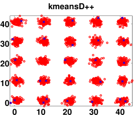
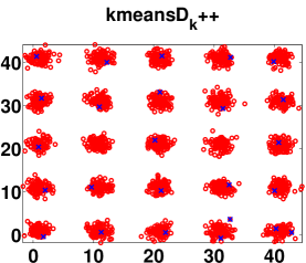
a) b) c)

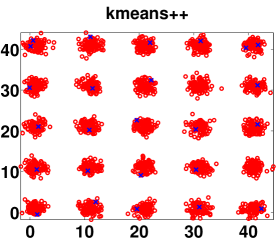
Figure 1: The seeds recovered by a) kmeansD++ b) kmeansD_k++ and c) kmeans++ initializers on a mixture of $25$ Gaussians.

kmeans++ versus kmeansD++

In this section we will show the fundamental difference between kmeans++ and kmeansD++ initializers. kmeans++ algorithm sampling the initial centroids (also called seeds) for the kmeans algorithm is summarized in Algorithm $1$. Here, $D(x)$ denotes the shortest Euclidean distance from a data point $x$ to the closest seed from among seeds already chosen ($S$). The kmeans++ initializer assigns the highest probability to the data point that is currently the furthest from its closest seed from among the set of seeds chosen already. kmeansD++ initializer chooses the seeds from among the points in the dataset using different probabilities of selecting a new member for set $S$. Before showing the algorithm, we will introduce notation. Let $K$ be the RBF kernel matrix with $(i,j)^{th}$ entrance equal to $K(i,j)=\exp(-\sigma\|x_{i}-x_{j}\|^{2})$ and $\sigma$ be a fixed positive constant (note that $K$ is of size $n\times n$ and is symmetric positive semi-definite), $K^{S}$ is a sub-matrix of matrix $K$ of size $|S|\times|S|$ defined by points from $S$, and $K^{S\cup\{x\}}$ is a sub-matrix of matrix $K$ of size $|S|+1\times|S|+1$ defined by points from $S\cup\{x\}$ (both sub-matrices are as well symmetric positive semi-definite). kmeansD++ algorithm is summarized in Algorithm $2$.

Input: dataset $\mathcal{X}$

1) $S=\emptyset$

2) Pick a point uniformly at random from $\mathcal{X}$ and add it to $S$.

3) for $i=1:1:k-1$:

a) choose data point $x\in\mathcal{X}$ at random with

probability $P(x|S)=\frac{D(x)^{2}}{\sum_{x^{{}^{\prime}}\in X}D(x^{{}^{\prime}})^{2}}$

b) $S=S\cup\{x\}$

Algorithm 1 kmeans++

Input: dataset $\mathcal{X}$
1, 2 and 4) as in kmeans++
3) for $i=1:1:k-1$:
choose data point $x\in\mathcal{X}$ at random with
probability $P(x|S)=\frac{det(K^{S\cup\{x\}})}{det(K^{S})}$

Algorithm 2 kmeansD++

kmeansD++ favors diversity by putting higher probability to sets of items that are diverse, which is the property that the kmeans++ initializer also has, however the former uses less aggressive initialization scheme, i.e. it does not necessarily put the highest probability to the data point that is currently the furthest from its closest seed from among the set of seeds chosen already. This can be shown by considering a simple example. Let $\mathcal{X}=\{x_{1},x_{2},x_{3}\}$ be the set of points on a $1D$ line, where $x_{1}$ was sampled first and then $x_{2}$ and $x_{3}$. We will consider two possible locations for $x_{3}$, that we will refer to as $x_{3}^{{}^{\prime}}$ and $x_{3}^{{}^{\prime\prime}}$, shown below:

a) $x_{1}$————–$0$————–$x_{2}$————–$x_{3}^{{}^{\prime}}$
b) $x_{1}$————–$0$————–$x_{2}$ and $x_{3}^{{}^{\prime\prime}}=0$

Let $\|x_{1}\|=\|x_{2}\|=D$ and $\|x_{3}^{{}^{\prime}}-x_{2}\|=D-\epsilon$ and let $D$ be fixed such that $D>\sqrt{\frac{\log 6}{4\sigma}}$. One can show that the DPP $k$-means initializer will put higher probability to select $x_{3}^{{}^{\prime}}$ then $x_{3}^{{}^{\prime\prime}}$, which is captured in Lemma 1. The proof is deferred to the appendix.

Lemma 1.

There exists $\epsilon\in(0,D)$ such that $P(x_{3}^{{}^{\prime}}|S)>P(x_{3}^{{}^{\prime\prime}}|S)$, thus kmeansD++ initializer can put the highest probability to the point which is not the furthest from the closest seed from among seeds already chosen.

Evaluation on synthetic datasets

$k_{t}$	4	9	16	25	36	100	Total
kmeansRand	1	3	6	8	14	31	63
kmeans++	0	1	2	2	2	9	16
kmeansDk++	0	1	1	2	4	10	18
kmeansD++	0	0	0	1	0	9	10
k	4	11	18	28	39	105

Table 1: Comparison of kmeansRand, kmeans++, kmeansD_k++ and kmeans++ initlializers on synthetic datasets. Number of clusters missed by each of the three algorithms. $k_{t}$ denotes the true number of clusters.

We compare kmeansRand, kmeans++, kmeansD++ and kmeansD_k++ initializers on standard synthetic data-sets. kmeansD_k++ refers to the kmeansD++ initializer run with pre-specified number of clusters ($k$). For these datasets we know the true number of clusters, denoted as $k_{t}$, and we well understand the geometry of the problem. We use mixture of well-separated Gaussians on a 2D grid. The variance of each Gaussian is $1$, the number of points in each of them is $100$ and the separation between them is $10$. The results are presented in Table 1 (for each experiment we report the median result over $50$ runs). For all the methods we report the number of missing clusters (missed). Furthermore, for the kmeansD++ initializer we report the number of clusters recovered automatically ($k)$. Additionally, in Figure 1 we show an exemplary result we obtained for a mixture of $25$ Gaussians. The results indicate that the performance of kmeansD++ and kmeans++ initializers are similar and furthermore kmeansD++ initializer is able to recover the true number of clusters underlying the data very accurately without having the number of clusters pre-specified (the correlation between $k_{t}$, the true $k$ and the $k$ predicted by kmeansD++ is 0.99). This highlights the ability of kmeansD++ to approximate the true $k$ – an ability that the kmeans++ initializer does not have.

Evaluation on real datasets

In this section, we compare the performance of the kmeans clustering algorithm initialized in two different ways, using the kmeansD++ initializer and using the kmeans++. The comparison is presented on three benchmark datasets: iris, ecoli and dermatology. The results are averaged over $50$ runs. Table 2 presents the F1-measures for clustering the three data-sets using kmeans++ and kmeansD_k++ (kmeansD++ with the number of clusters pre-specified). The results show that the F1-measures (considering the standard deviation) for the two clustering algorithms are comparable, which implies that kmeansD++ is empirically similar to kmeans++.

Datasets	$k_{t}$	kmeans++	kmeansDk++
iris	3	0.88$\pm$0.08	0.87$\pm$0.10
ecoli	8	0.56$\pm$0.06	0.63$\pm$0.06
dermatology	6	0.72$\pm$0.12	0.68$\pm$0.14

Table 2: F1-measure obtained by kmeans++ and kmeansD_k++ on benchmark datasets.

To highlight that kmeansD++ is able to automatically approximate the true $k$ while maintaining a good clustering performance, we compare the value of the kmeans clustering objective (called cost, lower is better) of kmeansD++ and kmeansD_k++. Note, we cannot report F1-measures for this evaluation since kmeansD++ automatically selects the number of clusters, which can be different from the true number of clusters.

Data	$k_{t}$	kmeansD++		kmeansDk++
		k	cost	cost
iris	3	3.80$\pm$0.41	62.60$\pm$9.19	92.94$\pm$27.16
ecoli	8	6.23$\pm$0.89	22.42$\pm$2.75	18.64$\pm$1.68
derm	6	32.63$\pm$0.52	2122.31$\pm$27.36	3824.52$\pm$282.51

Table 3: Performance of kmeansD++ and kmeansD_k++ on benchmark datasets. $k_{t}$ is the true number of clusters. $k$ is the number of clusters automatically approximated by kmeansD++. cost is the value of the kmeans objective.

Table 3 shows two results: 1) the $k$ predicted by kmeansD++ is close the true $k_{t}$ (columns 2 and 3) and 2) the quality of clustering in terms of the cost of kmeansD++ and kmeansD_k++ is comparable. The exception is the dermatology (derm) dataset, for which interestingly every feature has $34$ attributes which is very close to the number of clusters that kmeansD++ recovered. Since the DPP sampling algorithm uses the eigen-value decomposition, it seems that the sampler is mis-lead in thinking that data-set has $\sim 34$ classes. This behavior of the DPP sampler is interesting and requires further investigation (perhaps it is caused by weakly dependent features). Simultaneously, the $k$-means cost of the clusterings recovered by kmeansD++ on the dermatology dataset is significantly lower than the cost of kmeansD_k++. Note that it can be justified by the fact that when kmeansD++ resp. largely overestimates/underestimates $k$, the $k$-means cost of kmeansD++ should be resp. lower/higher than kmeansD_k++ because choosing resp. larger/smaller $k$ typically implies resp. smaller/larger average distance of a data point to its closest cluster center.

Evaluation on a Real Text Clustering Task

In Anonymous 2014, we introduced a novel task of automatically drawing xkcd movie narrative charts (right half of Figure 2) from textual screenplays (top left of Figure 2). We presented an end-to-end pipeline, employing algorithms from natural language processing, social network analysis and machine learning literature. The main focus of Anonymous 2014 was to present a novel task, its motivation, and a basic system pipeline. However, in this paper, we are only concerned with improving the key component of the pipeline – the text clustering module.

While for other text clustering tasks, heuristically setting $k$ may not be a major limitation, for the task at hand, it is critical that we have an automatic way of selecting (or approximating) $k$. This is because, in trying to cluster one data-set, it is well justified to use domain knowledge and human intuition to set $k$ or to refine $k$ by observing the output. However, for the task at hand, we need to find a clustering per movie. Since there are hundreds of movies, each with unique characteristics, heuristically setting $k$ is not feasible.

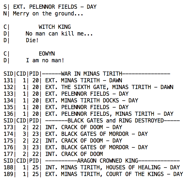
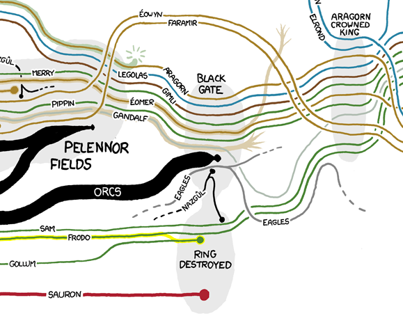
Figure 2: Right half: xkcd movie narrative chart for part of the movie Lord of the Rings. These charts show character interactions. The horizontal axis is time. The vertical grouping of lines indicates which characters are together at a given time. Source of image: http://xkcd.com/657/large/ Left top: snippet from the textual screenplay used as input for automatically creating the chart. Left bottom: scene boundaries and their scene identifier (SID), their cluster identifier (CID), and their plot identifier (PID).

Movie	# scenes (n)	# locations (gold $k$)	log(n)	$\sqrt{n}$	$k_{\textsc{kmeansD++}}$
Star Wars	137	35	2.13	11.7	41.98$\pm$3.30
The Last Crusade	148	57	2.17	12.16	47.72$\pm$3.50
Raiders of the Lost Ark	139	73	2.14	11.78	51.56$\pm$5.05
Pirates of the Caribbean	140	23	2.14	11.83	41.24$\pm$4.32
The Bourne Identity	160	74	2.20	12.64	61.98$\pm$5.03
Batman	209	77	2.32	14.45	71.42$\pm$5.14
Correlation with gold $k$	0.58	1	0.59	0.58	0.84

Table 4: List of movies, the number of scene boundaries, and the number of unique locations per movie in our test set (first three columns). Automatically selected $k$ by commonly used heuristic functions (next two columns). Automatically selected $k$ by using DPPs: mean and standard deviation over 50 runs (last two columns). Last row of the table shows the correlation between predicted $k$ and gold $k$.

Terminology and Task Definition

? (?) describe the structure of a movie screenplay. A screenplay is written using a strict formatting grammar. It has scene boundaries that textually separate scenes of a movie. Figure 2 shows some of the scene boundaries from the movie The Lord of the Rings. A scene boundary indicates whether the scene is to take place inside or outside (INT, EXT), the name of the location, and can potentially specify the time of day (e.g. DAY or NIGHT). The clustering task is to cluster scene boundaries (based on their lexical similarity) into $k$ clusters (with $k$ unknown). Since scene boundaries specify the location at which a scene is shot, the goal is to automatically determine the number and description of different scene locations in a movie (we remove tags INT./EXT., DAY/NIGHT before clustering).

Scene locations mentioned in scene boundaries are lexically similar, but not exactly the same. This is because a scene boundary, more often than not, describes a scene location, along with sub-location(s). For example, in Figure 2, the scene location Minas Tirith, which is a city, has multiple sub-locations such as “DOCKS” and “HOUSES OF HEALING”. Moreover, there are inconsistencies in the scene location descriptions. For example, some scene location descriptions for Pelennor Fields, which is a sub-location associated with Minas Tirith, are present as “PELENNOR FIELDS/MINAS TIRITH”, whereas others are present as “PELENNOR FIELDS”. As a consequence, a simple exact string matching algorithm is insufficient to find scene boundaries that belong to one location.

Data

To prepare a gold standard for this evaluation, we trained two human annotators to read a screenplay and mark all scenes (or scene boundaries) that belong to one location with a unique integer (which we refer to as cluster identifier). For example, in Figure 2, one of our annotators marked scene boundaries (sid) from 131 through 136 with cluster (or location) identifier (cid) 1. This means that all these scenes take place at one location, namely Minas Tirith. While performing the annotation task, the annotators used world knowledge that Pelennor Fields is a sub-location of Minas Tirith and thus should be marked with the same cluster identifier. Since we are clustering based on lexical similarity, to put lexically dissimilar strings Pelennor Fields and Minas Tirith together, our algorithm relies on the fact that they are mentioned together in a few scene boundaries (as is the case – see scene number 136).

After a few rounds of training we asked our annotators to fully annotate the screenplay for the movie Pirates of the Caribbean: Dead Man’s Chest. They achieved a high agreement of 0.86. We then asked our annotators to divide the remaining set of screenplays into half, each responsible for one half.

Table 4 gives the list of movies we annotated, along with the number of scenes and number of locations in each movie. We use these screenplays for evaluating our methodology.

Evaluation and Results

We calculate lexical (or string) similarity using a contiguous word kernel (?). We compare three ways of sampling the initial centroids for the kmeans algorithm: kmeansRand, kmeans++, and kmeansD++.

To set $k$ for kmeansRand, we employ common heuristics used in the literature: $k=\log(n)$ or $\sqrt{n}$, where $n$ is the number of data points. Table 4 presents the predicted number of $k$ using the functions $\log(n)$, $\sqrt{n}$. We run kmeansD++ 50 times and report the mean and standard deviation of the number of initial centroids selected by the DPP sampling algorithm automatically. The last row of table 4 shows the correlation of the predicted $k$ with the gold $k$ for the three methods. Deciding $k$ using DPPs has a significantly higher correlation with the gold $k$ (0.84) as compared to other standard methods (0.59 and 0.58). Note that the correlation of the number of scenes and the gold $k$ is low (0.58), so any monotonic function of the number of data-points will not have a much different correlation. This result shows that DPPs are well-suited for choosing $k$ for this data-set.

Next, we show that even if we provide the kmeans algorithm with the gold $k$, sampling using DPPs provides a better initialization, which results in a better clustering. Table 5 shows the macro-F1-measures for clustering obtained by three different ways of sampling the initial centroids. The numbers show that sampling using DPPs results in a significantly better clustering (higher F1-measure).

Movie	k	kmeansRand	kmeans++	kmeansDk++
Star Wars	35	0.61$\pm$0.04	0.62$\pm$0.02	0.63$\pm$0.04
Crusade	57	0.80$\pm$0.04	0.84$\pm$0.02	0.86$\pm$0.02
Raiders	73	0.68$\pm$0.03	0.76$\pm$ 0.02	0.77$\pm$ 0.02
Pirates	23	0.62$\pm$0.04	0.63$\pm$0.02	0.61$\pm$0.04
Bourne	74	0.64$\pm$0.03	0.69$\pm$0.03	0.68$\pm$0.05
Batman	77	0.62$\pm$0.03	0.63$\pm$0.02	0.66$\pm$0.03

Table 5: Mean and standard deviations of F1-measure on the test set.

Conclusion and Future Work

We conclude that kmeansD++ compares favorably to kmeans++ and performs better than kmeansRand with two additional advantages: it may be used in scenarios where explicit feature representation is absent and where the $k$ is unknown. In the future, we will attempt to prove approximation guarantees with respect to the $k$-means clustering objective for the kmeansD++ algorithm.

Appendix

First, we will show a useful lemma that we will use later.

Lemma 2.

There exists $\epsilon\in(0,D)$ such that

$$\exp(-2\gamma D^{2}(1\!-\!\frac{\epsilon}{D})^{2})-\exp(-2\gamma D^{2})\!<\!\frac{\exp(-2\gamma D^{2})}{2}$$ (1)

Proof.

For a fixed $D$ this result is straight-forward. ∎

Proof of Lemma 1.

$x_{1}$, $x_{2}$ and $x_{3}$ are respectively the first, second and third data point chosen by the kmeansD++ initializer. Thus we have that

$$P(x_{2}|S=x_{1})=\frac{det(K^{x_{2}\cup x_{1}})}{det(K^{x_{1}})}=1-\exp(-2\sigma\|x_{1}-x_{2}\|^{2})$$

and

$$P(x_{3}|S=x_{1}\cup x_{2})=\frac{det(K^{x_{1}\cup x_{2}\cup x_{3}})}{det(K^{x_{1}\cup x_{2}})}$$

$$=1-\frac{1}{1-\exp(-2\sigma\|x_{1}-x_{2}\|^{2})}\cdot\{\exp(-2\sigma\|x_{2}-x_{3}\|^{2})$$

$$+\exp(-2\sigma\|x_{1}-x_{3}\|^{2})$$

$$-2\exp(-\sigma(\|x_{1}-x_{2}\|^{2}+\|x_{2}-x_{3}\|^{2}+\|x_{1}-x_{3}\|^{2}))\}$$

Note that since $\|x_{1}-x_{2}\|=2D$, $\|x_{3}^{{}^{\prime}}-x_{2}\|=D-\epsilon$, $\|x_{3}^{{}^{\prime}}-x_{1}\|=3D-\epsilon$, $\|x_{3}^{{}^{\prime\prime}}-x_{2}\|=D$ and $\|x_{3}^{{}^{\prime\prime}}-x_{1}\|=D$, the following chain of inequlities are equivalent:

$$P(x_{3}^{{}^{\prime}}|S)>P(x_{3}^{{}^{\prime\prime}}|S)$$

$$\Longleftrightarrow\exp(-2\sigma(3D-\epsilon)^{2})+\exp(-2\sigma(D-\epsilon)^{2})$$

$$-2\exp(-\sigma(4D^{2}+(3D-\epsilon)^{2}+(D-\epsilon)^{2}))$$

$$\leq 2\exp(-2\sigma D^{2})-2\exp(-6\sigma D^{2})$$

$$\Longleftrightarrow\exp(-18\sigma D^{2}(1-\frac{\epsilon}{3D})^{2})+\exp(-2\sigma D^{2}(1-\frac{\epsilon}{D})^{2})$$

$$-2\exp(-\sigma(4D^{2}+(3D-\epsilon)^{2}+(D-\epsilon)^{2}))$$

$$\leq 2\exp(-2\sigma D^{2})-2\exp(-6\sigma D^{2})$$

We want to prove that the last inequality holds. We will show that by instead showing the series of stronger inequalities that hold and imply the above one. Note, that the inequality that implies the above one is given below

$$\exp(-18\sigma D^{2}(1-\frac{\epsilon}{3D})^{2})+\exp(-2\sigma D^{2}(1-\frac{\epsilon}{D})^{2})$$

$$\leq 2\exp(-2\sigma D^{2})-2\exp(-6\sigma D^{2})$$ (2)

This inequality can be rewritten as

$$2\exp(-6\sigma D^{2})+\exp(-18\sigma D^{2}(1-\frac{\epsilon}{3D})^{2})$$

$$+\exp(-2\sigma D^{2}(1-\frac{\epsilon}{D})^{2})\leq 2\exp(-2\sigma D^{2})$$

Recall that $\epsilon<D$ thus

$$1-\frac{\epsilon}{3D}>\frac{2}{3}\Longleftrightarrow\exp(-18\sigma D^{2}(1-\frac{\epsilon}{3D})^{2})<\exp(-8\sigma D^{2})$$

Thus, an even stronger inequality than the one in Equation 2 is the following one

$$2\exp(-6\sigma D^{2})+\exp(-8\sigma D^{2})$$

$$+\exp(-2\sigma D^{2}(1-\frac{\epsilon}{D})^{2})<2\exp(-2\sigma D^{2})$$ (3)

The inequality in Equation 3 implies the inequality in Equation 2. Note that $\exp(-8\sigma D^{2})\leq\exp(-6\sigma D^{2})$ thus one can construct an even stronger inequality given in Equation 4, than the one in Equation 3 that directly implies Equation 3 and therefore also Equation 2.

$$3\exp(\!-6\sigma D^{2})\!+\!\exp(\!-2\sigma D^{2}(1\!\!-\!\!\frac{\epsilon}{D})^{2})\!\leq\!2\exp(\!-2\sigma D^{2})$$ (4)

Recall that

$$D>\sqrt{\frac{\log 6}{4\sigma}}\Longleftrightarrow 3\exp(-6\sigma D^{2})<\frac{1}{2}\exp(-2\sigma D^{2})$$

Finally, we will below provide the last inequality, in Equation 5, which is the strongest from all discussed before as, if it holds, it directly implies the inequalities in Equation 4 and therefore also Equation 3 and 2.

$$\frac{\exp(-2\sigma D^{2})}{2}+\exp(-2\sigma D^{2}(1-\frac{\epsilon}{D})^{2})<2\exp(-2\sigma D^{2})$$ (5)

This equality can be equivalently rewritten as

$$\exp(-2\sigma D^{2}(1-\frac{\epsilon}{D})^{2})-\exp(-2\sigma D^{2})<\frac{\exp(-2\sigma D^{2})}{2},$$

where the last inequality holds by Lemma 1. ∎

References

- [Aggarwal, Deshpande, and Kannan 2009] Aggarwal, A.; Deshpande, A.; and Kannan, R. 2009. Adaptive sampling for k-means clustering. In APPROX.
- [Ailon, Jaiswal, and Monteleoni 2009] Ailon, N.; Jaiswal, R.; and Monteleoni, C. 2009. Streaming k-means approximation. In NIPS.
- [Aloise et al. 2009] Aloise, D.; Deshpande, A.; Hansen, P.; and Popat, P. 2009. Np-hardness of euclidean sum-of-squares clustering. Machine Learning 75(2):245–248.
- [Arthur and Vassilvitskii 2007] Arthur, D., and Vassilvitskii, S. 2007. k-means++: the advantages of careful seeding. In SODA.
- [Beygelzimer, Kakade, and Langford 2006] Beygelzimer, A.; Kakade, S.; and Langford, J. 2006. Cover trees for nearest neighbor. In ICML.
- [Bubeck, Meila, and von Luxburg 2012] Bubeck, S.; Meila, M.; and von Luxburg, U. 2012. How the initialization affects the stability of the k-means algorithm. ESAIM: Probability and Statistics 16:436–452.
- [Charikar et al. 1997] Charikar, M.; Chekuri, C.; Feder, T.; and Motwani, R. 1997. Incremental clustering and dynamic information retrieval. In STOC.
- [Choromanska and Monteleoni 2012] Choromanska, A., and Monteleoni, C. 2012. Online clustering with experts. In AISTATS.
- [Choromanska et al. 2013] Choromanska, A.; Jebara, T.; Kim, H.; Mohan, M.; and Monteleoni, C. 2013. Fast spectral clustering via the nyström method. In ALT.
- [Dempster, Laird, and Rubin 1977] Dempster, A. P.; Laird, N. M.; and Rubin, D. B. 1977. Maximum likelihood from incomplete data via the em algorithm. Journal of the Royal Statistical Society, Series B 39(1):1–38.
- [Guha et al. 2003] Guha, S.; Meyerson, A.; Mishra, N.; Motwani, R.; and O’Callaghan, L. 2003. Clustering data streams: Theory and practice. IEEE Trans. on Knowl. and Data Eng. 15(3):515–528.
- [Kang 2013] Kang, B. 2013. Fast determinantal point process sampling with application to clustering. In NIPS.
- [Kanungo et al. 2002] Kanungo, T.; Mount, D. M.; Netanyahu, N. S.; Piatko, C. D.; Silverman, R.; and Wu, A. Y. 2002. A local search approximation algorithm for k-means clustering. In Symposium on Computational Geometry, 10–18.
- [Kulesza and Taskar 2012] Kulesza, A., and Taskar, B. 2012. Determinantal point processes for machine learning. arXiv:1207.6083.
- [Kuncheva and Vetrov 2006] Kuncheva, L. I., and Vetrov, D. P. 2006. Evaluation of stability of k-means cluster ensembles with respect to random initialization. IEEE Transactions on Pattern Analysis and Machine Intelligence 28(11):1798–1808.
- [Liang and Klein 2009] Liang, P., and Klein, D. 2009. Online em for unsupervised models. In NAACL.
- [Lloyd 2006] Lloyd, S. 2006. Least squares quantization in pcm. IEEE Trans. Inf. Theor. 28(2):129–137.
- [Lodhi et al. 2002] Lodhi, H.; Saunders, C.; Shawe-Taylor, J.; Christianini, N.; and Watkins, C. 2002. Text classification using string kernels. The Journal of Machine Learning Research 2:419–444.
- [Rakhlin and Caponnetto 2006] Rakhlin, A., and Caponnetto, A. 2006. Stability of -means clustering. In NIPS.
- [Reichart and Korhonen 2013] Reichart, R., and Korhonen, A. 2013. Improved lexical acquisition through dpp-based verb clustering. In Proceedings of the 51st Annual Meeting of the Association for Computational Linguistics (Volume 1: Long Papers), 862–872. Sofia, Bulgaria: Association for Computational Linguistics.
- [Shamir and Tishby 2008] Shamir, O., and Tishby, N. 2008. Model selection and stability in k-means clustering. In COLT.
- [Turetsky and Dimitrova 2004] Turetsky, R., and Dimitrova, N. 2004. Screenplay alignment for closed-system speaker identification and analysis of feature films. In Multimedia and Expo, 2004. ICME’04. 2004 IEEE International Conference on, volume 3, 1659–1662.
- [von Luxburg 2007] von Luxburg, U. 2007. A tutorial on spectral clustering. Statistics and Computing 17(4):395–416.
- [von Luxburg 2010] von Luxburg, U. 2010. Clustering stability: An overview. Found. Trends Mach. Learn. 2(3):235–274.