Zeroth law and nonequilibrium thermodynamics for steady states in contact

Abstract

We ask what happens when two nonequilibrium systems in steady state are kept in contact and allowed to exchange a quantity, say mass, which is conserved in the combined system. Will the systems eventually evolve to a new stationary state where certain intensive thermodynamic variable, like equilibrium chemical potential, equalizes following zeroth law of thermodynamics and, if so, under what conditions is it possible? We argue that an equilibrium-like thermodynamic structure can be extended to nonequilibrium steady states having short-ranged spatial correlations, provided that the systems interact weakly to exchange mass with rates satisfying a balance condition - reminiscent of detailed balance condition in equilibrium. The short-ranged correlations would lead to subsystem factorization on a coarse-grained level and the balance condition ensures both equalization of an intensive thermodynamic variable as well as ensemble equivalence, which are crucial for construction of a well-defined nonequilibrium thermodynamics. This proposition is proved and demonstrated in various conserved-mass transport processes having nonzero spatial correlations.

I Introduction

Zeroth law is the cornerstone of equilibrium thermodynamics. It states that, if two systems are separately in equilibrium with a third one, they are also in equilibrium with each other Kardar . An immediate consequence of the zeroth law is the existence of state functions - a set of intensive thermodynamic variables (ITV) which equalize for two systems in contact. For example, if two systems are allowed to exchange a conserved quantity, say mass, they eventually achieve equilibrium where chemical potential becomes uniform throughout the combined systems. The striking feature of this thermodynamic structure is that all equilibrium systems form equivalence classes where each class is specified by a particular ITV. Then a system, an element of a particular class, is related to any other system in the class by a property that they have the same value of the ITV.

We ask whether a similar thermodynamic characterization is possible in general for systems having a nonequilibrium steady state (NESS). Can equalization of an ITV, governing “equilibration” between two steady-state systems in contact, be used to construct such equivalence classes? The answer is nontrivial; in fact, it is not even clear if such a formulation is at all possible Casas ; Eyink1996 ; Kurchan_PRE1997 ; OonoPaniconi ; Barrat_PRL2000 ; Baranyai_PRE2000 ; Behringer_Nature2002 ; HayashiSasa_PRE2003 ; SasaTasaki_JStatPhys2006 ; Sasa2014 ; Dickman_PRE2014 . In this paper, we find an affirmative answer to this question, which can lead to a remarkable thermodynamic structure where a vast class of systems having a NESS form equivalence classes, equilibrium systems of course included.

There have been extensive studies in the past to find a suitable statistical mechanical framework for systems having a NESS Casas ; Eyink1996 ; OonoPaniconi ; Bertini_PRL2001 ; HayashiSasa_PRE2003 ; SasaTasaki_JStatPhys2006 ; Sasa2014 ; Dickman_PRE2014 ; Sasa_PRL2008 ; Komatsu_PRL2008 ; Bertin_PRL2006 . Though the studies have not yet converged to a universal picture, it has been realized that suitably chosen mass exchange rates at the contact could possibly lead to proper formulation of a nonequilibrium thermodynamics SasaTasaki_JStatPhys2006 ; Sasa2014 ; Bertin_PRL2006 ; Bertin_PRE2007 ; Pradhan_PRL2010 ; Pradhan1_PRE2011 . An appropriate contact dynamics is crucial because, without it, properties of mass fluctuations in a system would be different, depending on whether the system is in contact (grandcanonical) or not in contact (canonical) with other system; in other words, without an appropriate contact dynamics, canonical and grand canonical ensembles would not be equivalent Pradhan1_PRE2011 ; Mukamel_PRL2012 . The situation is analogous to that in equilibrium where equivalence of ensembles, a basic tenet of equilibrium thermodynamics, is ensured by the mass exchange rates which satisfy detailed balance with respect to the Boltzmann distribution. However in nonequilibrium, in the absence of a priori knowledge of microscopic steady-state structure, the intriguing questions, (a) whether there indeed exist a class of exchange rates which could lead to the construction of a well- defined nonequilibrium thermodynamics and (b) how the rates could be determined, are still unsettled.

Previous studies addressed some of these issues. However, the exact studies (Bertin_PRL2006, ; Bertin_PRE2007, ) were mostly confined to a special class of models, called zero range processes. These models have product-measure or factorized steady state and therefore do not have any spatial correlations. In other studies, a class of lattice gas models with nonzero spatial correlations were considered SasaTasaki_JStatPhys2006 ; Pradhan_PRL2010 ; Dickman_PRE2014 ; Dickman2_PRE2014 ; Pradhan2_PRE2011 and, for some particular choice of mass exchange rates, zeroth law was found to be obeyed. However, the mass exchange rates, even in the limit of slow exchange, alters the fluctuation properties of the individual systems, leading to the breakdown of equivalence between canonical and grandcanonical ensembles.

In this paper, we formulate necessary and sufficient condition for which equilibrium thermodynamics can be consistently extended to weakly interacting nonequilibrium steady-state systems having nonzero spatial correlations. Under this condition, zeroth law is obeyed and “equilibration” between two systems (labeled by $\alpha={{1}},{{2}}$) in contact can be characterized by equalization of an intensive thermodynamic variable which is inherently associated with the respective isolated system. To obtain such a thermodynamic structure, we require the following condition: Mass exchange from one system to the other should occur weakly across the contact with the exchange rates satisfying

$$\frac{u_{{{1}}{{2}}}(\varepsilon)}{u_{{{2}}{{1}}}(\varepsilon)}=e^{-\Delta F},$$ (1)

a reminiscent of detailed balance condition in equilibrium. Here $u_{\alpha\alpha^{\prime}}(\varepsilon)$ is the rate with which a mass of size $\varepsilon$ is transferred from system $\alpha$ to $\alpha^{\prime}$, and $\Delta F$ is the change in a nonequilibrium canonical free energy of the contact regions. In the limit of weak interaction between systems, the mass exchange rates are not necessarily small, but only that the mass exchange process do not affect the dynamics in the individual systems and spatial correlations between the systems vanishes. Note that Eq. 1 requires a free energy function inherent to individual isolated system to exist, which, we argue, is the case in a system having short-ranged spatial correlations. This free energy function can in principle be obtained from a fluctuation-response relation, analogous to fluctuation-dissipation theorems in equilibrium.

The notion of weak interaction is crucial to construct a well-defined nonequilibrium thermodynamics. Also in equilibrium, one implicitly assumes weak interaction where interaction energy between systems is taken to be vanishingly small so that bulk dynamics in an individual system remain unaffected by the other system which may be put in contact with the former. Likewise, weakly interacting nonequilibrium systems imply that dynamics in the individual systems remain unaffected even when two systems are kept in contact. The weak interaction limit, which essentially demands vanishing of correlations between two systems across the contact, is however not guaranteed by mere slow exchange of masses and vice versa. We demonstrate how the weak interaction limit can actually be achieved.

The organization of the paper is as follows. In section II.A, we discuss why an additivity property as in Eq. 8 is required for constructing a well-defined thermodynamic structure for nonequilibrium systems. In section II.B, we show that the coarse-grained balance condition (see Eq. 1) on mass exchange rates ensures the desired additivity property. In section III, through various previously studied models and their variants, we illustrate how the mass exchange rates can be explicitly constructed so that the balance condition Eq. 1 is satisfied. In section IV, we discuss that generic mass exchange rates, even in the limit of slow exchange, leads to the breakdown of equivalence between canonical and grandcanonical ensembles. At the end, we summarize with a few concluding remarks and open issues.

II Theory

II.1 General considerations

Let us consider two systems $\alpha={{1}},{{2}}$ of size $V_{\alpha},$ having mass variables ${\bf m}_{\alpha}\equiv\{m_{i}\geq 0\}$ defined at the sites $i\in V_{\alpha}.$ Each of the systems, while not in contact with each other (we refer to the situation as canonical ensemble), has a nonequilibrium steady state distribution

$${\cal P}_{\alpha}({\bf m}_{\alpha})=\frac{\omega_{\alpha}({\bf m}_{\alpha})}{W_{\alpha}(M_{\alpha},V_{\alpha})}\delta\left(M_{\alpha}-\sum_{i\in V_{\alpha}}m_{i}\right)$$ (2)

where $\omega_{\alpha}({\bf m}_{\alpha})$ is the steady-state weight of a microscopic configuration ${\bf m}_{\alpha}$ and

$$W_{\alpha}(M_{\alpha},V_{\alpha})=\int d{{\bf m}_{\alpha}}\omega_{\alpha}({\bf m}_{\alpha})\delta\left(M_{\alpha}-\sum_{i\in V_{\alpha}}m_{i}\right),$$

is the partition sum ($\int d{{\bf m}_{\alpha}}$ implies integral over all mass variables $m_{i}$ with $i\in V_{\alpha}$). The delta function ensures conservation of mass $M_{\alpha}=\sum_{i\in V_{\alpha}}m_{i}$, or mass density $\rho_{\alpha}=M_{\alpha}/V_{\alpha}$, of individual systems. The microscopic weight $\omega_{\alpha}({\bf m}_{\alpha})$ is the time-independent solution of Master equation governing the time evolution of the system in the configuration space of ${\bf m}_{\alpha}$ and in most cases is not known. On the other hand, when the systems ${{1}}$ and ${{2}}$ are in contact, mass exchange from one system to the other at the contact region breaks conservation of $M_{{{1}},{{2}}}$ whereas the total mass $M=M_{{{1}}}+M_{{{2}}}$ of the combined system remains conserved. We refer this situation as a grand canonical ensemble.

To have a consistent thermodynamic structure, it is necessary that individual systems themselves have well defined canonical free energy functions, $F_{{{1}},{{2}}}$ for systems $\alpha={{1}}$ or ${{2}}$. Moreover, this free energy function should not change due to the contact between the two systems. That is, free energy of the combined system $F=F_{{1}}+F_{{2}}$ is obtained by adding the corresponding canonical free energies of the individual systems and the macrostate, or the maximum probable state, is obtained by minimizing the total free energy function. This additivity property has the following immediate consequences: (i) Equalization of an intensive thermodynamic variable, (ii) a fluctuation-response relation and (iii) zeroth law; all of them follows from standard statistical mechanics Kardar .

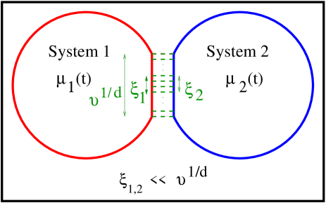
Figure 1: (Color online) Schematic representation: “Equilibration” of two steady-state systems in contact. Intensive thermodynamic variables $\mu_{1}(t)$ and $\mu_{2}(t)$, chemical potentials of systems $1$ and $2$ at time $t$, eventually equalize in the steady state, $\mu_{1}(t=\infty)=\mu_{2}(t=\infty)$. The size of the contact region $v^{1/d}$, $v$ the volume of the contact region in $d$ dimension, is much larger than the individual correlation length $\xi_{\alpha}$.

First we discuss the macroscopic properties of systems in canonical ensemble and how a free energy function can be defined consistently for nonequilibrium systems. We consider an individual system $\alpha$ divided into two subsystems, each of which being much larger than spatial correlation length $\xi_{\alpha}$ and total mass $M_{\alpha}$ being conserved. As subsystems much larger than the correlation lengths would be statistically independent in the thermodynamic limit, the steady state subsystem mass distribution can be written as product of some weight factors which depend only on mass of the individual subsystem Eyink1996 ; Bertin_PRL2006 . Thus, when $\xi_{{{1}},{{2}}}\ll v\ll V_{{{1}},{{2}}}$, we could view each individual system $\alpha$ composed of two statistically independent (apart from the constraint of total mass conservation provided by a delta function) macroscopically large subsystems - contact region (of size $v$ and mass $M_{\alpha}^{c}$) and the rest, i.e., the bulk (of size $V_{\alpha}-v$ and mass $M_{\alpha}^{b}=M_{\alpha}-M_{\alpha}^{c})$ - whose steady-state weights are factorized, i.e., product of two coarse-grained weights, as reflected in the partition sum

$$W_{\alpha}(M_{\alpha},V_{\alpha})\simeq\int dM^{c}_{\alpha}W_{\alpha}(M_{\alpha}-M^{c}_{\alpha})W_{\alpha}(M^{c}_{\alpha}).$$ (3)

Or equivalently, the joint probability distribution of subsystem masses will have a factorized form

$$P(M_{\alpha}^{c},M_{\alpha}^{b})\simeq\frac{W_{\alpha}(M_{\alpha}^{c})W_{\alpha}(M_{\alpha}^{b})}{W_{\alpha}(M_{\alpha},V_{\alpha})}\delta\left(M_{\alpha}-M_{\alpha}^{c}-M_{\alpha}^{b}\right)$$

$$=\frac{e^{-[F_{\alpha}(M_{\alpha}^{c})+F_{\alpha}(M_{\alpha}^{b})]}}{e^{-F_{\alpha}(M_{\alpha})}}\delta\left(M_{\alpha}-M_{\alpha}^{c}-M_{\alpha}^{b}\right),$$ (4)

which is maximized to obtain macrostate of the systems (i.e., the maximum probable state). These considerations immediately lead to the existence of a canonical free energy $F_{\alpha}\equiv-\ln W_{\alpha}$ in the steady state. The total steady-state free energy $F_{\alpha}(M_{\alpha},V_{\alpha})$ of the two subsystems is additive and is obtained by minimizing the sum of free energy of the bulk (of volume $V-v$) and that of the contact region (of volume $v$),

$$F_{\alpha}(M_{\alpha},V_{\alpha})={\rm inf}_{M_{\alpha}^{c}}[F_{\alpha}(M_{\alpha}^{c},v)+F_{\alpha}(M_{\alpha}-M_{\alpha}^{c},V_{\alpha}-v)].$$ (5)

The additivity property in Eq. 4 and the above minimization of total free energy implies existence of an intensive thermodynamic variable, called chemical potential,

$$\mu_{\alpha}(\rho_{\alpha})=\frac{\partial F_{\alpha}}{\partial M_{\alpha}}=\frac{\partial f_{\alpha}}{\partial\rho_{\alpha}}$$ (6)

which takes the same value for any subsystems (macroscopically large). In the above equation, we have defined a nonequilibrium free energy density function $f_{\alpha}(\rho_{\alpha})=F_{\alpha}/V_{\alpha}$.

Note that the nonequilibrium free energy function is defined in such a way that the principle of free energy minimization automatically holds. Interestingly, for a steady-state system having a conserved mass, this free energy function as well as chemical potential can be calculated from subsystem mass fluctuations (as illustrated later in various models) and therefore has practical importance, e.g., describing phase coexistence Pradhan2_PRE2011 ; Arghya , etc.

We next consider grandcanonical ensemble - a situation where mass exchange takes place between two systems through contact regions (see Fig. 1) each with volume $v$ (taken same for both systems for simplicity) which is much larger than finite spatial correlation length $\xi_{\alpha}$ but otherwise arbitrary. We demand that the canonical description where $M_{{1}}$ and $M_{2}$ are individually conserved, must be equivalent to the grand canonical ensemble where only total mass $M=M_{{{1}}}+M_{{{2}}}$ is conserved. That is, the microscopic weight of the combined system must be a product of the individual canonical microscopic weights and therefore the probability of a microscopic configuration of the combined system should be given by

$${\cal P}({\bf m}_{{{1}}},{\bf m}_{{{2}}})=\frac{\omega_{{{1}}}({\bf m}_{{{1}}})\omega_{2}({\bf m}_{2})}{W(M)}\delta\left(M-M_{{1}}-M_{{2}}\right),$$ (7)

with the the partition sum of the combined system being

$$W(M,V)=\int dM_{{{1}}}W_{{{1}}}(M_{1},V_{1})W_{{{2}}}(M-M_{1},V_{2}).$$

So the the joint distribution of individual system masses is also factorized and can be written as the product of the individual canonical weights,

$$P(M_{{{1}}},M_{{{2}}})=\frac{W_{{1}}(M_{{1}},V_{{1}})W_{{2}}(M_{{2}},V_{{2}})}{W(M,V)}$$

$$\times\delta\left(M-M_{{1}}-M_{{2}}\right),$$ (8)

and thus additivity is ensured for the combined systems. That is, total free energy $F(M,V)\equiv-\ln W(M,V)$ of the combined system in the steady state is given by

$$F(M,V)=\inf_{M_{{1}}}[F_{{1}}(M_{{1}},V_{{1}})+F_{{2}}(M-M_{{1}},V_{{2}})],$$

which is the sum of individual canonical free energies. This implies that the chemical potential equalizes upon contact, i.e., $\mu_{{1}}(\rho_{1})=\mu_{{2}}(\rho_{{2}})$.

II.2 Proof of the balance condition

Now we show how, in the weak interaction limit, the balance condition in Eq. 1 ensures additivity property in Eq. 8 - the main result of this paper. Let mass exchange occur at the contact with rate $u_{\alpha\alpha^{\prime}}(\varepsilon)$ where a mass $\varepsilon$ is transferred from system $\alpha$ to $\alpha^{\prime}$. The rate may depend on both the mass values at the two contact regions (the mass dependence not explicitly shown in $u_{\alpha\alpha^{\prime}}$). Mass conservation in the individual systems is then broken in this process ($M_{\alpha}\to M_{\alpha}-\varepsilon$ and $M_{\alpha^{\prime}}\to M_{\alpha^{\prime}}+\varepsilon$), generating a mass flow. To attain stationarity, average mass current $J_{{{1}}{{2}}}(\varepsilon)$ generated by all possible microscopic exchanges corresponding the rates $u_{{{1}}{{2}}}$, where the chipped off mass $\varepsilon$ flows from system ${{1}}$ to ${{2}}$, must be balanced by the reverse current $J_{{{2}}{{1}}}(\varepsilon)$. Note that, though the net steady-state current $|J_{\alpha\alpha^{\prime}}(\varepsilon)-J_{\alpha^{\prime}\alpha}(\varepsilon)|$ from one system to the other (across the contact) is exactly zero, the individual systems can still be far away from equilibrium and can have nonzero steady-state mass currents in the bulk.

Since the total mass $M=M_{{{1}}}+M_{{{2}}}$ of the combined system is conserved, the current balance condition $J_{{{1}}{{2}}}(\varepsilon)=J_{{{2}}{{1}}}(\varepsilon)$ can be written, using only one of the mass variables, say $M_{{{1}}}$, as

$$P(M_{{{1}}},M-M_{{{1}}})U_{{{1}}{{2}}}(M_{{1}},\varepsilon)=P(M_{{{1}}}-\varepsilon,M-M_{{{1}}}+\varepsilon)$$

$$\times U_{{{2}}{{1}}}(M-M_{{1}}+\varepsilon,\varepsilon).$$ (9)

Here $U_{\alpha\alpha^{\prime}}(x,y)$ is an effective rate with which mass $y$ is transferred from system $\alpha$, having mass $x$, to $\alpha^{\prime}$. The current balance, along with Eq. 8, gives

$$\frac{U_{{{1}}{{2}}}(M_{{1}},\varepsilon)}{U_{{{2}}{{1}}}(M-M_{{1}}+\varepsilon,\varepsilon)}=e^{-\Delta F}$$ (10)

where $\Delta F=\sum_{\alpha=1}^{2}(F_{\alpha}|_{final}-F_{\alpha}|_{initial}$) difference in free energy of the combined system. Or equivalently, we write the above ratio of effective exchange rates as

$$\frac{U_{{{1}}{{2}}}(M_{{1}},\varepsilon)}{U_{{{2}}{{1}}}(M-M_{{1}}+\varepsilon,\varepsilon)}=e^{(\mu_{\alpha}-\mu_{\alpha^{\prime}})\varepsilon},$$ (11)

where $\mu_{\alpha}=\partial F_{\alpha}/\partial M_{\alpha}$ is a nonequilibrium chemical potential (see Eq. 6) which is inherently associated with the individual system $\alpha$.

Next we obtain a condition on the actual microscopic exchange rate $u_{{{1}}{{2}}}(\varepsilon)$. We first use the expression of current $J_{\alpha\alpha^{\prime}}(\varepsilon)=\langle u_{\alpha\alpha^{\prime}}\rangle$ as the average mass transfer rate from system $\alpha$ to $\alpha^{\prime}$ and write $J_{{{1}}{{2}}}(\varepsilon)=\int\int d{\bf m}_{{1}}d{\bf m}_{{2}}{\cal P}({\bf m}_{{{1}}},{\bf m}_{{{2}}})u_{{{1}}{{2}}}(\varepsilon)$ as given below

$$J_{{{1}}{{2}}}(\varepsilon)=\left[\prod_{\alpha=1}^{2}\int d{\bf m}_{\alpha}\right]{\cal P}({\bf m}_{{{1}}},{\bf m}_{{{2}}})u_{{{1}}{{2}}}(\varepsilon)\delta(M-\sum_{\alpha=1}^{2}M_{\alpha})$$

$$=\frac{1}{W(M,V)}\int\int d{\bf m}_{{{1}}}d{\bf m}_{{{2}}}\omega_{{{1}}}({\bf m}_{{{1}}})\omega_{{{2}}}({\bf m}_{{{2}}})u_{{{1}}{{2}}}(\varepsilon)$$

$$\times\delta\left(M_{{{1}}}-\sum_{i\in V_{{{1}}}}m_{i}\right)\delta\left(M_{{{2}}}-\sum_{i\in V_{{{2}}}}m_{i}\right)\delta(M-\sum_{\alpha=1}^{2}M_{\alpha})$$

$$\simeq\frac{1}{W(M,V)}\int\int d{M^{c}_{{{1}}}}d{M^{c}_{{{2}}}}u_{{{1}}{{2}}}W_{{{1}}}(M^{c}_{{{1}}})W_{{{2}}}(M^{c}_{{{2}}})$$

$$\times W_{{{1}}}(M_{{{1}}}-M^{c}_{{{1}}},V_{{{1}}}-v)W_{{{2}}}(M_{{{2}}}-M^{c}_{{{2}}},V_{{{2}}}-v).\mbox{~{}~{}}$$ (12)

In the last step, we inserted an identity $\int d{M^{c}_{\alpha}}\delta(M^{c}_{\alpha}-\sum_{i\in v}m_{i})=1$, where $v$ being denoted here as the contact region in system $\alpha$, and then used the factorization property,

$$\int d{{\bf m}_{\alpha}}w_{\alpha}({\bf m}_{\alpha})\delta\left(M_{\alpha}-\sum_{i\in V_{\alpha}}m_{i}\right)\delta\left(M^{c}_{\alpha}-\sum_{i\in v}m_{i}\right)$$

$$\simeq W_{\alpha}(M^{c}_{\alpha},v)W_{\alpha}(M_{\alpha}-M^{c}_{\alpha},V_{\alpha}-v),$$

as in Eq. 3. As demonstrated later in various models in section III, the above factorization property is expected to be valid when the size of the contact region is much larger than the spatial correlation length $\xi_{\alpha}$ in system $\alpha$, i.e., when $v\gg(\xi_{\alpha})^{d}$ in $d$ dimension. Then, after some straightforward manipulations, we write $U_{{{1}}{{2}}}(M_{{1}},\varepsilon)=J_{{{1}}{{2}}}(\varepsilon)/P(M_{1},M_{2})$ as

$$U_{{{1}}{{2}}}(M_{{1}},\varepsilon)=\int_{\varepsilon}\int_{0}d{M_{{1}}^{c}}d{M_{{2}}^{c}}u_{{{1}}{{2}}}(\varepsilon)\prod_{\alpha=1}^{2}\frac{W_{\alpha}(M_{\alpha}^{c})e^{\mu_{\alpha}M_{\alpha}^{c}}}{{\cal Z}_{\alpha}},\mbox{~{}~{}}$$ (13)

by using Eq. 8 and using the following equality

$$W_{\alpha}(M^{c}_{\alpha})\frac{W_{\alpha}(M_{\alpha}-M^{c}_{\alpha},V_{\alpha}-v)}{W_{\alpha}(M_{\alpha},V_{\alpha})}=\frac{W_{\alpha}(M^{c}_{\alpha})e^{\mu_{\alpha}M^{c}_{\alpha}}}{{\cal Z}_{\alpha}}$$

where ${\cal Z}_{\alpha}=\int dM_{\alpha}^{c}~{}W_{\alpha}(M^{c}_{\alpha})~{}e^{\mu_{\alpha}M_{\alpha}^{c}}$. Similarly, the effective reverse exchange rate, corresponding to the transition $\{M^{c}_{{{1}}}-\varepsilon,M^{c}_{{{2}}}+\varepsilon\}\rightarrow\{M^{c}_{{{1}}},M^{c}_{{{2}}}\}$, can be written as

$$U_{{{2}}{{1}}}(M-M_{{1}}+\varepsilon,\varepsilon)=e^{(\mu_{{{2}}}-\mu_{{{1}}})\varepsilon}\int_{\varepsilon}\int_{0}d{M^{c}_{{{1}}}}d{M^{c}_{{{2}}}}u_{{{2}}{{1}}}(\varepsilon)$$

$$\times\frac{W_{{{1}}}(M^{c}_{{{1}}}-\varepsilon)e^{\mu_{{{1}}}M^{c}_{{{1}}}}}{{\cal Z}_{1}}\frac{W_{{{2}}}(M^{c}_{{{2}}}+\varepsilon)e^{\mu_{{{2}}}M^{c}_{{{2}}}}}{{\cal Z}_{2}}.~{}~{}$$ (14)

Now, substituting Eqs. 13 and 14 in Eq. 11 and then by equating the integrals which is valid for any functional form of weight factor $W_{\alpha}(m)$, we get the desired balance condition as in Eq. 1,

$$\frac{u_{{{1}}{{2}}}}{u_{{{2}}{{1}}}}=\frac{W_{{{1}}}(M^{c}_{{{1}}}-\varepsilon)}{W_{{{1}}}(M^{c}_{{{1}}})}\frac{W_{{{2}}}(M^{c}_{{{2}}}+\varepsilon)}{W_{{{2}}}(M^{c}_{{{2}}})}=e^{-\Delta F^{c}}=e^{-\Delta F}.~{}~{}$$ (15)

In the last step, we used the free energy of the contact region $F_{\alpha}^{c}(M_{\alpha}^{c})=-\ln W_{\alpha}(M^{c}_{\alpha})$ and equate the change in free energy at the contact $\Delta F^{c}=\sum_{\alpha=1}^{2}\Delta F_{\alpha}^{c}$ to the change in total free energy of the combined system $\Delta F$. This is so since the total free energy $F=\sum_{\alpha=1}^{2}(F^{c}_{\alpha}+F^{b}_{\alpha})$ can be written as a sum of bulk free energy $F^{b}_{\alpha}$ and contact free energy $F^{c}_{\alpha}$ where $\Delta F^{b}_{\alpha}=0$ (i.e., changes occur only at the contact regions). Note that the balance condition holds only at the contact regions for mass transfer from one system to the other. However, there is no detailed balancing in the bulk, except when both the systems are in equilibrium.

The balance condition in Eq. 15 is necessary and sufficient to ensure that the steady state has the required product form as in Eq. 7. This is because any contact dynamics which is constrained by the balance condition in Eq. 15 indeed satisfies Master equation in the steady state as the mass-current balance condition $J_{{{1}}{{2}}}(\varepsilon)=J_{{{2}}{{1}}}(\varepsilon)$, used for deriving the balance condition Eq. 1, is nothing but the balancing of configuration-space current occurring due to exchange of masses. This completes the proof.

Note that Eq. 15 does not uniquely specify the contact dynamics (CD); two simple choices which we discuss in this paper are given below,

$${\rm CD~{}I} : u_{\alpha\alpha^{\prime}}=u_{0}p(\varepsilon)\frac{W_{\alpha}^{c}(M^{c}_{\alpha}-\varepsilon)}{W_{\alpha}^{c}(M^{c}_{\alpha})},$$ (16)

$${\rm CD~{}II} : u_{\alpha\alpha^{\prime}}=u_{0}p(\varepsilon){\rm Min}\{1,e^{-\Delta F}\},$$ (17)

where $u_{0}$ an arbitrary constant (not necessarily small) and $p(\varepsilon)$ is a probability that mass $\varepsilon$ is chosen for exchange. Note that the limit $u_{0}\rightarrow 0$ implies slow exchange of masses. The case with $u_{0}=0$ implies no exchange of masses, i.e., the systems are kept isolated. The resemblance between the rate in Eq. 17 and the familiar Metropolis rate is indeed striking. In equilibrium, Eq. 15 reduces to the condition of detailed balance, albeit on a coarse- grained level. A similar notion of coarse-grained detailed balance was previously envisaged in Bertin_PRE2007 , though in the context of zero range processes which do not have any spatial correlations.

What still remains to be done is to explicitly specify the exchange rates satisfying Eq. 15. This requires calculation of the subsystem weight factor $W_{\alpha}(m,v)$ in a particular system of interest, which can be done following Ref. PRL2014 . Note that the Laplace transform $\tilde{W}_{\alpha}(s,v)=\int_{0}^{\infty}W_{\alpha}(M^{c}_{\alpha})\exp(-sM^{c}_{\alpha})dM^{c}_{\alpha}$ of the subsystem weight factor can be written in terms of the Laplace transform $\tilde{W}_{\alpha}(s,V_{\alpha})=\int_{0}^{\infty}W_{\alpha}(M_{\alpha},V_{\alpha})\exp(-sM_{\alpha})dM_{\alpha}$ of the individual canonical partition sum $W_{\alpha}(M_{\alpha},V_{\alpha})$ as

$$\tilde{W}_{\alpha}(s,v)=\left[\tilde{W}_{\alpha}(s,V_{\alpha})\right]^{v/V_{\alpha}},$$ (18)

in the limit $V_{\alpha}\gg v\gg\xi_{\alpha}^{d}$ (in $d$ dimensions). The partition sum $W_{\alpha}(M_{\alpha},V_{\alpha})$ can be calculated, as follows, from a canonical fluctuation-response relation. The subsystem mass fluctuation when calculated in canonical ensemble with $u_{0}=0$ is related to the change in density $\rho_{\alpha}$ in response to the change in chemical potential $\mu_{\alpha}$ (as in Eq. 6) as given below

$$\frac{d\rho_{\alpha}}{d\mu_{\alpha}}={\psi_{\alpha}(\rho_{\alpha})},$$ (19)

where, for subsystem volume $v\gg\xi_{\alpha}^{d}$, the function $\psi_{\alpha}(\rho_{\alpha})=\sigma^{2}_{v}/v$ with variance of subsystem mass $\sigma_{v}^{2}=\langle{(M_{\alpha}^{c})}^{2}\rangle-v^{2}\rho_{\alpha}^{2}$. The variance of subsystem mass in system $\alpha$ can be calculated from the knowledge of correlation function $c_{\alpha}(r)$ as $\sigma^{2}_{v}\simeq v\sum_{r=-\infty}^{r=\infty}c_{\alpha}(r)$ where $c_{\alpha}(r)=\langle m_{i}m_{i+r}\rangle-\rho_{\alpha}^{2}$ is the two-point correlation between masses at sites $i$ and $i+r$ PRL2014 . We assumed here that the correlation function $c_{\alpha}(r)$ is short-ranged or sufficiently rapidly decaying function so that it is integrable, which is usually the case when there is no long-ranged correlations in the systems. Therefore, once the functional dependence of $\psi_{\alpha}(\rho_{\alpha})$ on the respective density is known, the partition sum for individual system $W_{\alpha}(M_{\alpha},V_{\alpha})=\exp[-V_{\alpha}f_{\alpha}(\rho_{\alpha})]$, $f_{\alpha}(\rho_{\alpha})$ being nonequilibrium free energy density, can be obtained by first integrating the fluctuation-response relation Eq. 19 w.r.t. density $\rho_{\alpha}$ and then integrating chemical potential as given in Eq. 6. Then the subsystem weight factor $W_{\alpha}(m)$ can be obtained, via inverse Laplace transform, from Eq. 18.

We emphasize here that, even when the detailed microscopic weight $\omega_{\alpha}({\bf m}_{\alpha})$ is not known, the subsystem weight factor $W_{\alpha}(m,v)$ can still be obtained, either analytically or numerically, from the subsystem mass fluctuations or equivalently from the two-point spatial correlation functions; this makes our formulation work both in theory and in practice.

III Models and Illustrations

In this section, we illustrate our analytical results in nonequilibrium models studied extensively in the past as well as in their variants. For each of these models, we analytically obtain chemical potential $\mu(\rho_{\alpha})$ and the weight factor $W_{\alpha}(m)$ when the system is isolated (i.e., $u_{0}=0$), and then we explicitly construct the mass exchange rates $u_{\alpha\alpha^{\prime}}$ so that they satisfy the balance condition Eq. 15. Using these rates, we perform simulations (we use both the contact dynamics I and II). Our simulations demonstrate that, when two systems are kept in contact with unequal initial individual chemical potentials, they indeed “equilibrate” where the chemical potentials associated with the respective isolated systems equalize in the final steady state of the combined system.

III.1 Zero Range Processes

For completeness, we first consider zero range processes (ZRP) Haney2005 which have a factorized steady state (FSS). For ZRP, a well-defined thermodynamic structure has been previously constructed Bertin_PRE2007 . Consider two systems $\alpha={{1}},{{2}}$ where their steady-state weights

$$\omega_{\alpha}({\bf m}_{\alpha})=\prod_{i\in V_{\alpha}}h_{\alpha}(m_{i})$$

are simply product of factors $h_{\alpha}(m_{i})$, function of only single-site mass variable. The individual systems exactly satisfy Eq. 3 with weights of contact region (volume $v$) and the rest of system (volume $V_{\alpha}-v$) being $W_{\alpha}^{c}=(f_{\alpha})^{v}$ and $W_{\alpha}^{b}=(f_{\alpha})^{V_{\alpha}-v}$, respectively. When mass exchange occurs either with rate CD I (Eq. 16) or with rate CD II (Eq. 17), it is easy to check that the joint distribution, which satisfies Master equation, is given by

$${\cal P}({\bf m}_{1},{\bf m}_{2})\propto\prod_{\alpha}\prod_{i\in V_{\alpha}}\exp[-f_{\alpha}(m_{i})],$$

i.e., product of individual weight factors $\omega_{\alpha}({\bf m}_{\alpha})$ with $f_{\alpha}(m_{i})=-\ln h_{\alpha}(m_{i})$. Note that, for FSS, Eq. 15 indeed reduces to detailed balancing at the contact, as found in Bertin_PRE2007 .

III.2 Finite Range Processes

Now we consider a general situation - keeping in contact systems having nonzero spatial correlations. To this end, we introduce a broad class of analytically tractable models, for simplicity in one dimension, where a particle (or mass of size $\varepsilon$) is transferred stochastically from a site to one of its nearest-neighbours with rates depending on the discrete occupation numbers (or continuous mass variables) of $R$ neighbouring sites. These models are direct generalization of the zero range processes PRL2014 ; Amit and are called here finite range processes, with range $R$. These finite range mass transport processes have a clusterwise factorized steady state (CFSS) where each weight factor depends on the occupation numbers (or mass variables) $m_{i}$ ($i\in R$) of a cluster of size $R$. We consider two systems $\alpha={{1}},{{2}}$, for simplicity on two one dimensional periodic lattices of individual size $L_{\alpha}$, where each system having a CFSS of form

$$\omega_{\alpha}({\bf m}_{\alpha})=\prod_{i=1}^{L_{\alpha}}g_{\alpha}(m_{i},m_{i+1},\dots,m_{i+R})$$

where $g_{\alpha}$ a function of $R+1$ mass or occupation variables at consecutive $R+1$ sites. Clearly, $R=0$ corresponds to the factorized steady state (FSS) as in ZRP. The CFSS could arise in a variety of mass transport processes where mass chipping rate in the bulk satisfies certain conditions, details of which will be provided elsewhere Amit . Below, we consider only the continuous mass CFSS.

Unlike ZRP, the joint distribution of masses is not factorized on the single-site level as $g(m_{i},m_{i+1},\dots,m_{i+R})$ is function of masses at $R+1$ sites and therefore generates finite spatial correlations. In this paper, mainly due to analytical tractability, we consider a special form of $g_{\alpha}(m_{i},m_{i+1},\dots,m_{i+R})$ which is a homogeneous function,

$$g_{\alpha}(\Gamma m_{i},\Gamma m_{i+1},\dots,\Gamma m_{i+R})=\Gamma^{\delta}g_{\alpha}(m_{i},m_{i+1},\dots,m_{i+R})$$ (20)

with $\delta$ real. For this particular form, the two-point correlation function $c_{\alpha}(r)$ can be exactly calculated. By rescaling of mass variable $m_{k}=\rho_{\alpha}m^{\prime}_{k}$ in the individual isolated system with density $\rho_{\alpha}$, correlation of masses $\langle m_{i}m_{i+r}\rangle$ at sites $i$ and $i+r$ can be written, as $\langle m_{i}m_{i+r}\rangle=A_{\alpha}(r)\rho_{\alpha}^{2}$ where

$$A_{\alpha}(r)=\frac{\prod_{k}\left[\int_{0}^{\infty}dm^{\prime}_{k}g_{\alpha}^{(k)}(\{m^{\prime}_{k}\}_{{}_{R}})\right]m^{\prime}_{i}m^{\prime}_{i+r}\delta\left(\sum_{k}m^{\prime}_{k}-L_{\alpha}\right)}{\prod_{k}\left[\int_{0}^{\infty}dm^{\prime}_{k}g_{\alpha}^{(k)}(\{m^{\prime}_{k}\}_{{}_{R}})\right]\delta\left(\sum_{k}m^{\prime}_{k}-L_{\alpha}\right)},$$ (21)

$g_{\alpha}^{(k)}(\{m^{\prime}_{k}\}_{{}_{R}})\equiv\rho_{\alpha}^{-\delta}g_{\alpha}(m_{k},m_{k+1}\dots,m_{k+R})$ PRL2014 . The function $A_{\alpha}(r)$ depends on relative distance $r$, but is independent of density $\rho_{\alpha}$, and can be exactly calculated using a transfer matrix method Amit . Then, in an individual system $\alpha$, we obtain variance in a subsystem of size $v$ as $\sigma^{2}_{v}=v\rho_{\alpha}^{2}/\eta_{\alpha}$ with $\eta_{\alpha}^{-1}=\sum_{r=-\infty}^{\infty}[A_{\alpha}(r)-1]$. Now the subsystem weight factor $W_{\alpha}(m)$ can be exactly calculated, using the method outlined in the end of section II.B, to get a functional form of $W_{\alpha}(m)=m^{v\eta_{\alpha}-1}$.

In the case of nonzero spatial correlations, by considering a system in a coarse-grained level, one can have physical insights into the role of the balance condition Eq. 1. Let us divide a system $\alpha$ into $\nu_{\alpha}=V_{\alpha}/v$ number of almost statistically independent subsystems of equal volume $v$ with subsystem masses labelled by ${\bf\cal M}_{\alpha}\equiv\{{\cal M}_{\alpha,j}\}$, provided that the spatial correlation length $\xi_{\alpha}$ is much smaller than $v^{1/d}$ (in $d$ dimensions). Then the joint probability distribution of the subsystem masses of systems $\alpha$ are factorized:

$${\cal P}(\{{\bf\cal M}_{{{1}}},{\bf\cal M}_{{{2}}}\})\propto\prod_{\alpha}\prod_{j\in V_{\alpha}}\exp[-F^{(\alpha)}(\{{\cal M}_{\alpha,j}\})]$$

where free energy $F_{\alpha}=-\sum_{j}\ln W_{\alpha}({\cal M}_{\alpha,j})$ of system $\alpha$ is additive over the subsystems. Now let two such systems ${{1}}$ and ${{2}}$ be kept in contact such that mass from one specific subsystem of ${{1}}$ participate in a microscopic mass-exchange dynamics with its adjacent subsystem of ${{2}}$ with rates satisfying Eq. 15. In a coarse-grained level, as the subsystems could be considered as sites, the systems effectively become a set of sites with an “FSS”, where mass exchange occurs between two adjacent sites (here subsystems) with rates satisfying balance condition Eq. 15, and therefore the additivity property in Eq. 8 holds exactly in the limit of large subsystem volume $v\gg\xi_{{{1}},2}$.

Next, we discuss in detail a special case of the clusterwise factorized steady state with $R=1$.

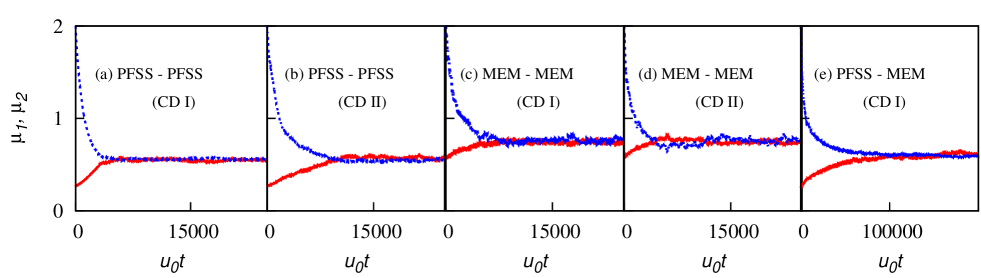
Figure 2: (Color online) “Equilibration” of steady states in contact: In (a)-(e), chemical potentials $\mu_{{1}}(t)$ and $\mu_{{2}}(t)$ of systems ${{1}}$ (red solid lines) and ${{2}}$ (blue dotted lines) vs. rescaled time $u_{0}t$. $\mu_{{1}}$ and $\mu_{{2}}$, initially chosen to be different, eventually equalize. Densities ($\rho_{{1}}$, $\rho_{{2}}$) in the final steady states are respectively ($3.60$, $5.40$) in (b), ($3.57$, $5.43$) in (c), ($5.31$, $2.69$) in (d), ($5.32,2.68$) in (e), and ($3.32$, $6.68$) in (f). In all cases, $p(\varepsilon)=p_{b}(\varepsilon)=\exp(-\varepsilon)$, $u_{0}=0.1$ and $v=10$ (except in (d) and (e) where $v=1$).

III.3 Pair Factorized Steady State (PFSS)

To demonstrate that our results are valid even in the presence of nonzero spatial correlations, we first consider two one-dimensional periodic lattices of $L_{\alpha}$ sites with continuous mass variable $m_{i}\geq 0$ at sites $i=1,2,\dots,L_{\alpha}.$ The following mass conserving dynamics in the bulk leads to a CFSS with $R=1$, usually called pair factorized steady state (PFSS) Evans_PRL2006 , where mass $\varepsilon$ chosen from a distribution $p_{b}(\varepsilon)$ is chipped off from a site $i$ and transferred to its right neighbor with rate

$$u_{\alpha}^{b}(\varepsilon)=p_{b}(\varepsilon)\frac{g_{\alpha}(m_{i-1},m_{i}-\varepsilon)}{g_{\alpha}(m_{i-1},m_{i})}\frac{g_{\alpha}(m_{i}-\varepsilon,m_{i+1})}{g_{\alpha}(m_{i},m_{i+1})},$$ (22)

which depends on the masses at the departure site and its nearest neighbors, and on the chipped-off mass $\varepsilon$. Since, in this case, mass-transfer happens in only one direction in the bulk, there are nonzero bulk currents present in the individual systems. We consider homogeneous $g_{\alpha}(x,y)=\Gamma^{-\delta}g_{\alpha}(\Gamma x,\Gamma y),$ for which one can exactly calculate $\psi_{\alpha}(\rho_{\alpha})=\rho_{\alpha}^{2}/\eta_{\alpha}$ and values of $\eta_{\alpha}$ for various microscopic parameters Amit . Then following the method outlined in section II.B, we analytically obtain $W_{\alpha}(m)=m^{v\eta_{\alpha}-1}$ and chemical potential $\mu_{\alpha}=-\eta_{\alpha}/\rho_{\alpha}$ where $\eta_{\alpha}$ depends on $\delta$. When two such systems are kept in contact, mass conservation in individual system is broken and both density $\rho_{\alpha}(t)$ and corresponding chemical potential $\mu_{\alpha}(t)$ evolve until a stationarity is reached where the net mass current from one system to another vanishes and densities are adjusted so that chemical potentials equalize. We simulate using $g_{\alpha}(x,y)=(x^{\delta}+y^{\delta}+cx^{\gamma}y^{\delta-\gamma})$ and allow the two PFSS with $\eta_{1}=2$ ($\delta=1$, $c=0$) and $\eta_{2}=3$ ($\delta=2$, $c=1$, $\gamma=3/2$) to exchange mass following CD I (and CD II in different simulations) with $u_{0}=0.1$, $p(\varepsilon)=p_{b}(\varepsilon)=exp(-\varepsilon)$ and $L_{{1}}=L_{{2}}=1000$. The contact volume $v=10$ is taken much larger than $\xi_{\alpha}$ which is here only about a couple of lattice spacings. Simulations in Figs. 2(a) and 2(b) demonstrate that, starting from arbitrary initial densities, the combined system reaches a stationary state where $\mu_{1}=\mu_{{2}}.$

The equalization of an ITV, i.e., the above mentioned chemical potential, indeed implies zeroth law which we verify next for three steady states having a PFSS: PFSS$1$ ($\delta=1$, $c=0$; $\eta_{1}=2$), PFSS$2$ ($\delta=3$, $c=0$; $\eta_{2}=4$) and PFSS$3$ ($\delta=2$, $c=1.0$, $\gamma=3/2$; $\eta_{3}=3$) with CD I. First, PFSS$1$ with density $\rho_{1}\simeq 3.60$ and PFSS$2$ with density $\rho_{2}\simeq 7.25$ are separately equilibrated with a third system PFSS$3$ with density $\rho_{3}\simeq 5.37$. Then, PFSS$1$ with density $\rho_{1}$ and PFSS$2$ with density $\rho_{2}$ are brought into contact. The two resulting densities after equilibration remain almost unchanged, confirming zeroth law. The zeroth law can be similarly verified for CD II.

III.4 Mass Exchange Models (MEM)

There are numerous examples MajumdarPRL1998 ; KrugGarcia2000 ; RajeshMajumdar2000 ; Zielen_JSP2002 ; Mohanty_JSTAT2012 , where nonequilibrium processes with a conserved mass show short-ranged spatial correlations, but the exact steady-state structures are not known. How does one find a contact dynamics which ensures Eq. 8 in these cases? We address the question in a class of widely studied nonequilibrium mass transport processes KMP1982 ; CC2000 ; Matthes-Toscani_JStatPhys2008 ; Yakovenko_RMP2009 , as another demonstration of how our formulation can be implemented in practice. In these models, we call them mass exchange models (MEM), in one dimension the continuous masses $m_{i}\geq 0$ and $m_{i+1}\geq 0$ at randomly chosen nearest neighbors $i$ and $i+1$ respectively are updated from time $t$ to $t+dt$ as

$$m_{i}(t+dt)=\lambda_{\alpha}m_{i}(t)+r(1-\lambda_{\alpha})m_{sum}(t),$$

$$m_{i+1}(t+dt)=\lambda_{\alpha}m_{i+1}(t)+(1-r)(1-\lambda_{\alpha})m_{sum}(t),$$

where, $m_{sum}=m_{i}+m_{i+1}$ is the sum of nearest neighbor masses, $r$ is a random number uniformly distributed in $[0,1]$, and $0<\lambda_{\alpha}<1$ a model dependent parameter. As the spatial correlations are nonzero but very small, the subsystem weight factor in the steady states of individual systems can be obtained, to a very good approximation, as $W_{\alpha}(m)=m^{v\eta_{\alpha}-1}$ with $\eta_{\alpha}=(1+2\lambda_{\alpha})/(1-\lambda_{\alpha})$ PRL2014 . In panels (c) and (d) of Fig. 2, we observe equalization of chemical potentials $\mu_{{1}}(t)=-\eta_{{1}}/\rho_{{1}}(t)$ and $\mu_{{2}}(t)=-\eta_{{2}}/\rho_{{2}}(t)$ (respective ITV in this case) of systems $1$ and $2$ respectively for both contact dynamics I and II and for $u_{0}=0.1$, $v=1$, $L_{{1}}=L_{{2}}=100$ and $p(\varepsilon)=p_{b}(\varepsilon)=\exp(-\varepsilon)$. The zeroth law can be readily verified for MEM as done in the case of PFSS.

There is no particular difficulty when systems having different kind of bulk dynamics are in contact; equilibration occurs as long as there is a common conserved quantity which is exchanged following Eq. 15. We demonstrate this in panel (e) of Fig. 2, taking two systems, PFSS and MEM, in contact where mass exchange dynamics at the contact is governed by CD I. In this case, chemical potentials $\mu_{{1}}(t)$ and $\mu_{{2}}(t)$ eventually equalize and zeroth law follows.

IV Equivalence of ensembles

In the previous section, we have demonstrated that, when two nonequilibrium systems with short-ranged correlation are allowed to exchange a conserved quantity following a contact dynamics conditioned by Eq. 1, they indeed evolve to a stationary state where an intensive thermodynamic variable (ITV), which is inherently associated with the respective isolated system, equalizes. In this thermodynamic construction, zeroth law is obeyed and, at the same time, equivalence of ensembles is also maintained. However, note that mere equalization of an intensive thermodynamic variable, or validity of zeroth law, does not guarantee the balance condition Eq. 1 and is not enough to construct a consistent nonequilibrium thermodynamics. This is because the ITV which equalizes for systems in grandcanonical ensemble is not necessarily the ITV defined (using additivity property Eq. 4) for individual isolated systems in canonical ensemble. To construct a well-defined thermodynamic structure, one must ensure that these two ITVs are indeed the same. That is, one requires that the combined system (grandcanonical ensemble) is statistically equivalent to the individual isolated systems (canonical ensemble).

The requirement of ensemble equivalence, which essentially demands that the contact dynamics must not alter the fluctuation properties in the individual systems, is nothing special in nonequilibrium scenario; it has been an essential ingredient in constructing equilibrium thermodynamics. The proposed balance condition Eq. 1 precisely ensures these two aspects - in one hand, it ensures equalization of an intensive thermodynamic variable and, on the other hand, it guarantees ensemble equivalence.

Note that, unlike in equilibrium, when two nonequilibrium systems are brought into contact, the final steady state of the combined system depends, in general, on the absolute values of mass exchange rates, even if the ratio between forward and reverse exchange rates remains unchanged. In these cases too, in the limit of slow mass exchange ($u_{0}\rightarrow 0$) and weak interaction, there could exist an ITV which equalizes upon contact. However, in spite of the equalization of an ITV, as we illustrate in the following subsections, the mass exchange rates which do not satisfy the balance condition Eq. 1 lead to the breakdown of ensemble equivalence. That is, mass fluctuation in the isolated systems can be different from that in the combined system and, in that case, an equilibrium-like thermodynamic structure cannot be formulated.

In the examples given below, we consider weakly interacting lattice gases (driven and nondriven both) which exchange masses infinitesimally slowly, i.e., $u_{0}\rightarrow 0$. The limit of slow exchange is useful in exactly calculating the mass fluctuations as the inhomogeneities which could occur in the contact regions of the individual systems is avoided and the weak interaction limit is also achieved.

IV.1 Lattice gases

We start with $d$-dimensional lattice gases with interacting particles, obeying hardcore exclusion (at most one particle at a site). We consider periodic boundaries, though the following analysis can be straightforwardly extended to other boundary conditions (e.g., reflecting boundary, discussed in the case of nearest-neighbour- exclusion lattice gases in section IV.B). Internal dynamics: Particles hop, from one site to its nearest neighbour, inside the individual systems according to some specified rates, e.g., rates satisfying local detailed balance KLS with respect to the Boltzmann distribution $\sim\exp(-\beta E)$ where $\beta$ inverse temperature, $E_{\alpha}$ energy function of system $\alpha$ and $E=E_{{1}}+E_{{2}}$ total energy. Mass exchange or contact dynamics: The rate with which a particle at the contact region (which could be localized, even a point or single-site contact or global contact) jumps from system $\alpha$ to $\alpha^{\prime}$, provided the contact site in $\alpha$ is occupied and the contact site in $\alpha^{\prime}$ is unoccupied, is simply a constant $u_{0}p_{\alpha}$. There is no additional constraint on these rates except that $u_{0}\rightarrow 0$ so that particle exchange occurs very slowly.

Since the transition rates overall do not satisfy detailed balance, the probability of a microscopic configuration of the combined system is not given by the Boltzmann distribution $\sim\exp(-\beta E)$. Note that the particle hopping rates inside the individual systems remain the same irrespective of two systems being in contact or not, which is necessary in realizing the weak interaction limit (which, for a finite $u_{0}$, is however not sufficient).

The joint probability distribution $P(M_{{1}},M_{{2}})$ of particle numbers $M_{{1}}$ and $M_{{2}}$ of individual systems, i.e., the large deviation function governing mass or particle-number fluctuations, can be exactly calculated using the general recursion relation Eq. 9, with setting $\varepsilon=1$ (i.e., one- particle transfer at a time), as

$$P(M_{{1}},M_{{2}})=P(0,M)\prod_{M_{{1}}}\frac{U_{{{2}}{{1}}}(M_{{2}}+1,1)}{U_{{{1}}{{2}}}(M_{{1}},1)}\delta(M-\sum_{\alpha=1}^{2}M_{\alpha})$$

$$=P(0,M)\left[e^{\sum_{M_{{1}}=0}^{M_{{1}}}(\ln U_{{{2}}{{1}}}-\ln U_{{{1}}{{2}}})}\right]\delta(M-\sum_{\alpha=1}^{2}M_{\alpha}).~{}~{}~{}$$ (23)

Now writing the effective mass exchange rates $U_{{{1}}{{2}}}=u_{0}p_{{1}}\rho_{{1}}(1-\rho_{2})$ and $U_{{{2}}{{1}}}=u_{0}p_{2}\rho_{{2}}(1-\rho_{1})$ and integrating over densities, the joint mass distribution can be exactly written in the form as given below,

$$P(M_{{1}},M_{{2}})\propto e^{-\left[V_{{1}}f_{{1}}+V_{{2}}f_{{2}}\right]}\delta(M-V_{{1}}\rho_{{1}}-V_{{2}}\rho_{{2}})$$ (24)

where free energy densities $f_{{1}}=\int_{0}^{\rho_{{1}}}\mu_{{1}}d\rho_{{1}}$ and $f_{{2}}=\int_{M/V_{1}}^{\rho_{{2}}}\mu_{{2}}d\rho_{{2}}$ with chemical potential given by

$$\mu_{\alpha}(\rho_{\alpha})=\ln p_{\alpha}+\ln\frac{\rho_{\alpha}}{1-\rho_{\alpha}}.$$ (25)

It is somewhat surprising that the joint mass distribution, as in Eq. 23 or 24, is actually independent of the internal dynamics in each systems. Moreover, the above free energy and chemical potential are nothing but those of a noninteracting hardcore lattice gas. The macrostate, or the maximum probable state, of the combined system with final steady-state densities in the individual systems can be obtained by minimizing the total free energy $F=V_{{1}}f_{{1}}+V_{2}f_{{2}}$, with the constraint $V_{{1}}\rho_{{1}}+V_{{2}}\rho_{{2}}={\rm constant}$. In other words, there exists an intensive thermodynamic variable, we call chemical potential, which indeed equalizes upon contact, i.e., $\mu_{{1}}(\rho_{{1}})=\mu_{{2}}(\rho_{{2}})$. The equalization of chemical potential essentially signifies the steady-state current balance between two systems across the contact as encoded in Eq. 9 and moreover this immediately leads to zeroth law under this particular contact dynamics.

However, in the above construction, clearly there is breakdown of equivalence between canonical and grandcanonical ensembles and, therefore thermodynamically, the construction is not well-defined. Note that, in this case, the free energy and chemical potential are not the same as those defined in canonical ensemble (see Eq. 4) when $u_{0}=0$. In fact, in the canonical ensemble, subsystem particle-number fluctuation in individual systems can have nontrivial properties due to the presence of inter-particle interactions. But, with the above contact dynamics, the particle-number fluctuation in the grand-canonical ensemble is governed by a chemical potential of a noninteracting hardcore lattice gas (see Eq. 25), which is so in spite of the presence of inter-particle interaction in the individual systems. The origin of the discrepancy in fluctuations in the two cases with $u_{0}=0$ and $u_{0}\rightarrow 0$ lies in the fact that mass exchange rates do not satisfy the balance condition Eq. 1, which drastically changes the fluctuation properties of the systems in grandcanonical ensembles. That is, unless the balance condition Eq. 1 is satisfied by the mass exchange rates, the cases with $u_{0}=0$ and $u_{0}\rightarrow 0$ are always different.

For example, inequivalence of ensembles arises in the previous studies SasaTasaki_JStatPhys2006 ; Pradhan_PRL2010 ; Pradhan2_PRE2011 where two driven lattice gases are allowed to exchange particles with some exchange rates, which were chosen on an ad hoc basis. To be specific, let us consider the systems studied in Pradhan2_PRE2011 , where two lattice gases - a nondriven lattice gas ${{1}}$ and a driven lattice gas ${{2}}$ (Katz- Lebowitz-Spohn model KLS ), are kept in contact. Particle hopping rates in the bulk as well as the particle exchange rates across the contact both satisfy a local detailed balance KLS . In the limit of slow mass exchange, the ratio of the effective transition rates was found, to a good approximation, to be Pradhan2_PRE2011

$$\frac{U_{{{1}}{{2}}}}{U_{{{2}}{{1}}}}=\frac{e^{\mu_{{1}}(\rho_{{1}})}}{e^{\mu_{{2}}(\rho_{2})}}$$

where $\mu_{{1}}(\rho_{1})$ and $\mu_{2}(\rho_{2})$ are functions of respective density. By substituting this ratio in Eq. 23 and then integrating over densities, one readily obtains the joint distribution $P(M_{{1}},M_{{2}})$ of particle numbers $M_{{1}}$ and $M_{{2}}$, which has exactly the same form as given in Eq. 24. Then, minimizing total free energy function, one can identify $\mu_{{1}}(\rho_{{1}})$ and $\mu_{{2}}(\rho_{{2}})$ as chemical potentials which equalize in the final steady state after the systems are brought into contact; the equalization of this chemical potential was indeed verified through simulations in Pradhan2_PRE2011 . However, the microscopic exchange rates $u_{\alpha\alpha^{\prime}}$ have not been derived from the canonical fluctuation-response relation Eq. 19 and therefore are not constrained by the balance condition Eq. 1. Consequently, as in the previous example, these exchange rates lead to the breakdown of ensemble equivalence. That is, free energy function and chemical potential for systems in grandcanonical ensemble are not the same as those for isolated systems in canonical ensemble.

IV.2 Lattice gases with nearest neighbour exclusion

Next we consider previously studied athermal hardcore lattice gases, in two dimensions, with nearest neighbour exclusion (NNE) Dickman_PRE2014 ; Dickman2_PRE2014 . We study the simplest case where particles can be exchanged through a single-site or point-wise contact ($v=1$) in each system, which can be readily generalized to other cases, e.g, when particles are exchanged globally ($v=V$) or in higher dimensions. The transition rates for particles hopping inside the individual systems (irrespective of that they are isolated or in contact with each other) can be chosen to be some specific nearest neighbour or next-nearest neighbour (or mixture of both) hopping rates in the presence of a driving field $D$; details of these rates, which can be found in Dickman_PRE2014 ; Dickman2_PRE2014 , are omitted here as they are not explicitly required in the following analysis as long as the systems exchange particles very slowly.

Let us keep two such lattice gases, systems $\alpha={{1}}$ and ${{2}}$, in contact with each other Dickman_PRE2014 ; Dickman2_PRE2014 where particles are exchanged as follows. A site is called open if the site as well as all its nearest neighbours are unoccupied. Provided the contact site, say in system ${{1}}$, is occupied and the contact site in system ${{2}}$ is open, the particle from system ${{1}}$ is transferred to system ${{2}}$ with rate $u_{0}\rightarrow 0$. The joint distribution $P(M_{{1}},M_{{2}})$ of masses $M_{{1}}$ and $M_{{2}}$ in the individual systems can be straightforwardly calculated by substituting $U_{\alpha\alpha^{\prime}}(M_{\alpha},\varepsilon)=\rho^{c}_{\alpha}\rho_{\alpha^{\prime}}^{\rm c,op}$ (with $\varepsilon=1$) in Eq. 23 where $\rho^{c}_{\alpha}$ and $\rho_{\alpha^{\prime}}^{\rm c,op}$ are probabilities that contact site is occupied in system $\alpha$ and open in system $\alpha^{\prime}$, respectively. Note that the probabilities $\rho^{c}_{\alpha}({\bf x_{c}},\rho_{\alpha})$ and $\rho_{\alpha}^{\rm c,op}({\bf x_{c}},\rho_{\alpha})$ are, in principle, functions of the location ${\bf x_{c}}$ of the contact site as well as of the global density $\rho_{\alpha}$ in system $\alpha$.

Then the joint distribution has the same form as given in Eq. 24 where free energy densities can be written as $f_{{1}}(\rho_{{1}})=\int_{0}^{\rho_{{1}}}\mu_{{1}}d\rho_{{1}}$ and $f_{{2}}(\rho_{{2}})=\int_{M/V_{1}}^{\rho_{{2}}}\mu_{{2}}d\rho_{{2}}$ with chemical potentials given by

$$\mu_{\alpha}(\rho_{\alpha})=\ln\left(\frac{\rho^{c}_{\alpha}}{\rho_{\alpha}^{\rm c,op}}\right).$$ (26)

The macrostate is obtained by minimizing total free energy function $F=V_{{1}}f_{{1}}(\rho_{{1}})+V_{{2}}f_{{2}}(\rho_{{2}})$ with the constraint $V_{{1}}\rho_{{1}}+V_{{2}}\rho_{{2}}={\rm constant}$, leading to the existence of an intensive thermodynamic variable, i.e., chemical potential, which indeed equalizes upon contact, $\mu_{{1}}(\rho_{{1}})=\mu_{{2}}(\rho_{2})$. However, the functional form of the chemical potentials do depend on the boundary conditions. Because, a particular boundary condition can make the density profile nonuniform and, consequently, the quantities $\rho^{c}_{\alpha}({\bf x_{c}},\rho_{\alpha})$ and $\rho_{\alpha}^{\rm c,op}({\bf x_{c}},\rho_{\alpha})$ not only depend on density $\rho_{\alpha}$ but also on the location ${\bf x_{c}}$ of the contact site.

For example, in the case of periodic boundary condition and uniform bulk hopping rates where the system remains homogeneous, chemical potential is given by

$$\mu_{\alpha}=\ln\left(\frac{\rho_{\alpha}}{\rho^{\rm op}_{\alpha}}\right),$$ (27)

where the density $\rho^{c}_{\alpha}({\bf x_{c}},\rho_{\alpha})=\rho_{\alpha}$ at the contact site ${\bf x_{c}}$ and the probability $\rho^{\rm c,op}_{\alpha}({\bf x_{c}},\rho_{\alpha})=\rho^{\rm c,op}_{\alpha}(\rho_{\alpha})$ of the contact site being open depends only on the bulk density $\rho_{\alpha}$, i.e., both $\rho^{c}_{\alpha}$ and $\rho^{\rm c,op}_{\alpha}$ do not depend on the location ${\bf x_{c}}$ of the contact. This is exactly the chemical potential which was found in Dickman_PRE2014 , using the concept of virtual exchange, for the pointwise (single-site contact with $v=1$) as well as for global exchanges ($v=V_{\alpha}=V_{\alpha^{\prime}}$).

On the other hand, for hard-wall or reflecting boundary condition (e.g., periodic boundary in $x$ direction and two hard walls placed along $x=1$ and $x=L$), the density profile becomes nonuniform and the chemical potential then depends on where the contact site is located. For example, if the contact site is located in the bulk, chemical potential has to be calculated with respect to the density and probability of open site in the bulk. That is, even in these cases of nonuniform systems, the existence of the above mentioned chemical potential would then apparently restore an equilibrium-like thermodynamic structure, as formulated in Dickman_PRE2014 ; Dickman2_PRE2014 where an ITV equalizes upon contact and zeroth law is obeyed.

In short, in all the above cases of weakly interacting NNE lattice gases with uniform or nonuniform density profiles, there indeed exists, in the limit of slow exchange, an ITV which equalizes upon contact and zeroth law is also obeyed. However, in each of these cases - depending on the boundary conditions and the location of contact site, the functional form of free energy and chemical potential of the individual systems in the grandcanonical ensembles are different. Of course, they are not the same as those defined for the individual isolated systems in canonical ensemble.

V Summary and Discussion

In this paper, we demonstrate that weakly interacting nonequilibrium systems, with short-ranged spatial correlations and having a common conserved quantity, e.g., mass which is exchanged upon contact between two systems, have an equilibrium-like thermodynamic structure in steady state, provided the rates of mass exchange between two systems satisfy a balance condition as given in Eq. 1. The size of the contact regions, otherwise arbitrary, should be much larger than correlation lengths, therefore making the contact regions effectively independent of the rest of the systems. The balance condition, reminiscent of equilibrium detailed balance on a coarse-grained level, leads to zeroth law of thermodynamics and fluctuation- response relations analogous to the equilibrium fluctuation- dissipation theorems. In other words, for mass exchange rates satisfying the balance condition, one can construct equivalence classes consisting of systems having a nonequilibrium steady state. The systems in each class are specified by the value of an intensive thermodynamic variable, inherently associated with the respective isolated systems, which does not change when any two systems in the class are allowed to exchange mass according to Eq. 1.

Following are the two most important aspects in the present study. Firstly, we constructed a well-defined thermodynamic structure, encompassing all (driven or nondriven) steady-state systems having nonzero, though short-ranged, spatial correlations. Secondly, we have identified the notion of weak interaction in constructing such a thermodynamic structure. Note the distinction between the limit of weak interaction and the limit of mere slow mass exchange; the former essentially implies vanishing of spatial correlations between two systems while in contact (ensuring that there is no inhomogeneities at the contact regions) and, moreover, leads to the additivity property as formulated in Eq. 8, provided that the balance condition Eq. 1 is satisfied.

In equilibrium, weak interaction directly translates into vanishingly small interaction energy between two systems in contact, i.e., sum of the internal energies of the individual systems equals to total internal energy of the combined system. However, in nonequilibrium, the microscopic weights are not determined by energy function and therefore even zero interaction energy could lead to nonzero spatial correlations between two systems while in contact, e.g., when mass exchange rates are finite or nonuniform. In principle, the weak-interaction limit can be achieved by keeping the bulk transition rates (i.e., the internal dynamics in the individual systems) unchanged, irrespective of whether the systems are in contact with each other or they are isolated. Weak interaction, which usually requires slow exchange of masses, is possible even when mass exchange rates are finite, e.g., when the balance condition Eq. 1 holds.

This thermodynamic construction, which is based on additivity property, may not be valid for the systems having a slow decaying long-ranged spatial correlation, e.g., two-point correlation function decaying as $1/r^{d}$ (or slower) in $d$ dimensions, which has been observed in a large class of driven systems Garrido ; Grinstein . In that case, the correlation function is not integrable and therefore the additivity property in Eq. 3 presumably breaks down, implying that the fluctuation-response relation in Eq. 19 may not exist. Nevertheless, as we demonstrated in this paper, the results will be applicable to a still wide class of driven systems which have short-ranged correlations. Moreover, even in the presence of long-ranged correlations when the strength of the correlations is weak, the additivity property, to a good approximation, could hold. This possibly explains why driven lattice gases, such as KLS models studied in Refs. HayashiSasa_PRE2003 ; SasaTasaki_JStatPhys2006 ; Pradhan_PRL2010 ; Dickman_PRE2014 , admit an approximate free energy and chemical potential, thus providing a quite good description of various steady state properties - including description of phase transitions Pradhan2_PRE2011 - albeit only in the limit of weak interaction.

It is important to note that slow exchange of masses does not necessarily imply weak interaction. For example, the nonuniformly driven athermal lattice gas studied in Dickman2_PRE2014 is one where the system is not actually weakly interacting, even when mass exchange rates are vanishingly small or slow. In a realistic scenario, finite interaction may be present between two systems while in contact. As an open issue, it remains to be seen whether, in the case of finite interaction, there exists an intensive thermodynamic variable which would equalize upon contact. Also, it would be interesting to explore the validity of additivity property in systems having boundary layers or hard walls, as their presence could alter the fluctuations in the bulk of a system which is otherwise isolated. A related important open question SasaTasaki_JStatPhys2006 is whether the thermodynamic structure based on additivity could be used to connect various physical observables, such as mechanical pressure on a wall Solon1 ; Solon2 or statistical forces on a probe Basu , to an intensive thermodynamic variable such as chemical potential. Though addressing the issue in full generality remains a formidable challenge, it would be worthwhile to identify a particular class of driven systems, if any, where connection between ‘mechanics’ and nonequilibrium thermodynamics could be established on a firmer ground.

We end the discussion with a concluding remark. The problem of constructing a well-defined thermodynamic structure in nonequilibrium, even when spatial correlations are short-ranged, is more subtle than that in equilibrium as, in nonequilibrium, zeroth law alone cannot ensure an equivalence class. Even when zeroth law holds, nonequilibrium ensembles (canonical and grandcanonical) may not be equivalent as the fluctuation properties of systems in grandcanonical ensemble depend on the details of contact dynamics as well as the boundary conditions - which gives insights into the conceptual difficulties in constructing a nonequilibrium thermodynamics, e.g., as attempted in SasaTasaki_JStatPhys2006 ; Dickman_PRE2014 ; Dickman2_PRE2014 ; Pradhan_PRL2010 ; Pradhan1_PRE2011 . In this scenario, our study provides a general prescription for dynamically generating different equivalent nonequilibrium ensembles and could thus help in formulating a well-defined nonequilibrium thermodynamics for driven systems in general.

VI Acknowledgement

SC acknowledges the financial support from the Council of Scientific and Industrial Research, India [Grant No. 09/575(0099)/2012-EMR-I]. PP and PKM acknowledge the financial support from the Science and Engineering Research Board (Grant No. EMR/2014/000719).

References

- (1) M. Kardar, Statistical Physics of Particles, Cambridge University Press (2007).
- (2) D. Jou, J. Casas-Vazquez and G. Lebon, Rep. Prog. Phys. 51, 1105 (1988). D. Jou and J. Casas-Vazquez, Phys. Rev. A 45, 8371 (1992).
- (3) G. L. Eyink, J. L. Lebowitz, H. Spohn, J. Stat. Phys 83, 385 (1996).
- (4) L. F. Cugliandolo, J. Kurchan, and L. Peliti, Phys. Rev. E 55, 3898 (1997).
- (5) Y. Oono and M. Paniconi, Prog. Theor. Phys. Suppl. 130, 29 (1998).
- (6) A. Barrat, J. Kurchan, V. Loreto, and M. Sellitto, Phys. Rev. Lett. 85, 5034 (2000).
- (7) A. Baranyai, Phys. Rev. E 62, 5989 (2000).
- (8) B. Behringer, Nature 415, 594 (2002).
- (9) K. Hayashi and S. Sasa, Phys. Rev. E 68, 035104 (2003).
- (10) S. Sasa and H. Tasaki, J. Stat. Phys. 125, 125 (2006).
- (11) T. S. Komatsu, N. Nakagawa, S. Sasa, and H. Tasaki, J. Stat. Phys. 159, 1237 (2015).
- (12) R. Dickman and R. Motai, Phys. Rev. E 89, 032134 (2014).
- (13) L. Bertini, A. De Sole, D. Gabrielli, G. Jona-Lasinio, C. Landim, Phys. Rev. Lett. 87, 040601 (2001). L. Bertini, A. De Sole, D. Gabrielli, G. Jona-Lasinio, C. Landim, J. Stat. Phys. 107, 635 (2002).
- (14) T. S. Komatsu, N. Nakagawa, S. Sasa, and H. Tasaki, Phys. Rev. Lett. 100, 230602 (2008).
- (15) T. S. Komatsu and N. Nakagawa, Phys. Rev. Lett. 100, 030601 (2008).
- (16) E. Bertin, O. Dauchot, and M. Droz, Phys. Rev. Lett. 96, 120601 (2006).
- (17) E. Bertin, K. Martens, O. Dauchot, and M. Droz, Phys. Rev. E 75, 031120 (2007).
- (18) P. Pradhan, C. P. Amann, and U. Seifert, Phys. Rev. Lett. 105, 150601 (2010).
- (19) P. Pradhan, R. Ramsperger, and U. Seifert, Phys. Rev. E 84, 041104 (2011).
- (20) O. Cohen and D. Mukamel, Phys. Rev. Lett. 108, 060602 (2012).
- (21) R. Dickman, Phys. Rev. E 90, 062123 (2014).
- (22) P. Pradhan, and U. Seifert, Phys. Rev. E 84, 051130 (2011).
- (23) A. Das, S. Chatterjee, P. Pradhan, and P. K. Mohanty, arXiv:1506.04647.
- (24) S. Chatterjee, P. Pradhan and P. K. Mohanty, Phys. Rev. Lett. 112, 030601 (2014).
- (25) M. R. Evans and T. Hanney, J. Phys. A 38, R195 (2005).
- (26) A. Chatterjee, P. Pradhan, and P. K. Mohanty, arXiv: 1505.05047.
- (27) M. R. Evans, T. Hanney, and S. N. Majumdar, Phys. Rev. Lett. 97, 010602 (2006).
- (28) S. N. Majumdar, S. Krishnamurthy, and M. Barma, Phys. Rev. Lett. 81, 3691–3694 (1998).
- (29) J. Krug and J. Garcia, J. Stat. Phys. 99, 31 (2000).
- (30) R. Rajesh and S. N. Majumdar, J. Stat. Phys. 99, 943 (2000).
- (31) F. Zielen and A. Schadschneider, J. Stat. Phys. 106, 173 (2002).
- (32) S. Bondyopadhyay and P. K. Mohanty, J. Stat. Mech. (2012) P07019.
- (33) C. Kipnis, C. Marchioro, and E. Presutti, J. Stat. Phys. 27, 65 (1982).
- (34) A. Chakraborti and B. K. Chakrabarti, Eur. Phys. J. B 17, 167 (2000).
- (35) D. Matthes and G. Toscani, J. Stat. Phys. 130, 1087 (2008).
- (36) V. M. Yakovenko and J. B. Rosser, Rev. Mod. Phys. 81, 1703 (2009).
- (37) S. Katz, J. L. Lebowitz, and H. Spohn, J. Stat. Phys. 34, 497 (1984).
- (38) Pedro L. Garrido, Joel L. Lebowitz, Christian Maes, and Herbert Spohn, Phys. Rev. A 42, 1954 (1990).
- (39) G. Grinstein, D.-H. Lee, and S. Sachdev, Phys. Rev. Lett. 64, 1927 (1990).
- (40) A. P. Solon, J. Stenhammar, R. Wittkowski, M. Kardar, Y. Kafri, M. E. Cates, J. Tailleur, Phys. Rev. Lett. 114, 198301 (2015).
- (41) A. P. Solon, Y. Fily, A. Baskaran, M. E. Cates, Y. Kafri, M. Kardar and J. Tailleur, Nat. Phys. (2015); arXiv:1412.3952.
- (42) U. Basu, C. Maes, K. Netocny, Phys. Rev. Lett. 114, 250601 (2015).