A provable SVD-based algorithm for learning topics in dominant admixture corpus

Abstract

Topic models, such as Latent Dirichlet Allocation (LDA), posit that documents are drawn from admixtures of distributions over words, known as topics. The inference problem of recovering topics from such a collection of documents drawn from admixtures, is NP-hard. Making a strong assumption called separability, [4] gave the first provable algorithm for inference. For the widely used LDA model, [6] gave a provable algorithm using clever tensor-methods. But [4, 6] do not learn topic vectors with bounded $l_{1}$ error (a natural measure for probability vectors).

Our aim is to develop a model which makes intuitive and empirically supported assumptions and to design an algorithm with natural, simple components such as SVD, which provably solves the inference problem for the model with bounded $l_{1}$ error. A topic in LDA and other models is essentially characterized by a group of co-occurring words. Motivated by this, we introduce topic specific Catchwords, a group of words which occur with strictly greater frequency in a topic than any other topic individually and are required to have high frequency together rather than individually. A major contribution of the paper is to show that under this more realistic assumption, which is empirically verified on real corpora, a singular value decomposition (SVD) based algorithm with a crucial pre-processing step of thresholding, can provably recover the topics from a collection of documents drawn from Dominant admixtures. Dominant admixtures are convex combination of distributions in which one distribution has a significantly higher contribution than the others. Apart from the simplicity of the algorithm, the sample complexity has near optimal dependence on $w_{0}$, the lowest probability that a topic is dominant, and is better than [4]. Empirical evidence shows that on several real world corpora, both Catchwords and Dominant admixture assumptions hold and the proposed algorithm substantially outperforms the state of the art [5].

1 Introduction

Topic models [1] assume that each document in a text corpus is generated from an ad-mixture of topics, where, each topic is a distribution over words in a Vocabulary. An admixture is a convex combination of distributions. Words in the document are then picked in i.i.d. trials, each trial has a multinomial distribution over words given by the weighted combination of topic distributions. The problem of inference, recovering the topic distributions from such a collection of documents, is provably NP-hard. Existing literature pursues techniques such as variational methods [2] or MCMC procedures [3] for approximating the maximum likelihood estimates.

Given the intractability of the problem one needs further assumptions on topics to derive polynomial time algorithms which can provably recover topics. A possible (strong) assumption is that each document has only one topic but the collection can have many topics. A document with only one topic is sometimes referred as a pure topic document. [7] proved that a natural algorithm, based on SVD, recovers topics when each document is pure and in addition, for each topic, there is a set of words, called primary words, whose total frequency in that topic is close to 1. More recently, [6] show using tensor methods that if the topic weights have Dirichlet distribution, we can learn the topic matrix. Note that while this allows non-pure documents, the Dirichlet distribution gives essentially uncorrelated topic weights.

In an interesting recent development [4, 5] gave the first provable algorithm which can recover topics from a corpus of documents drawn from admixtures, assuming separability. Topics are said to be separable if in every topic there exists at least one Anchor word. A word in a topic is said to be an an Anchor word for that topic if it has a high probability in that topic and zero probability in remaining topics. The requirement of high probability in a topic for a single word is unrealistic.

Our Contributions:

Topic distributions, such as those learnt in LDA, try to model the co-occurrence of a group of words which describes a theme. Keeping this in mind we introduce the notion of Catchwords. A group of words are called Catchwords of a topic, if each word occurs strictly more frequently in the topic than other topics and together they have high frequency. This is a much weaker assumption than separability. Furthermore we observe, empirically, that posterior topic weights assigned by LDA to a document often have the property that one of the weights is significantly higher than the rest. Motivated by this observation, which has not been exploited by topic modeling literature, we suggest a new assumption. It is natural to assume that in a text corpus, a document, even if it has multiple themes, will have an overarching dominant theme. In this paper we focus on document collections drawn from dominant admixtures. A document collection is said to be drawn from a dominant admixture if for every document, there is one topic whose weight is significantly higher than other topics and in addition, for every topic, there is a small fraction of documents which are nearly purely on that topic. The main contribution of the paper is to show that under these assumptions, our algorithm, which we call TSVD , indeed provably finds a good approximation in total $l_{1}$ error to the topic matrix. We prove a bound on the error of our approximation which does not grow with dictionary size $d$, unlike [5] where the error grows linearly with $d$.

Empirical evidence shows that on semi-synthetic corpora constructed from several real world datasets, as suggested by [5], TSVD substantially outperforms the state of the art [5]. In particular it is seen that compared to [5] TSVD gives $27$% lower error in terms of $L_{1}$ recovery on $90$% of the topics.

Problem Definition:

$d,k,s$ will denote respectively, the number of words in the dictionary, number of topics and number of documents. $d,s$ are large, whereas, $k$ is to be thought of as much smaller. Let ${\cal S}_{k}=\{x=(x_{1},x_{2},\ldots,x_{k}):x_{l}\geq 0;\sum_{l}x_{l}=1\}$. For each topic, there is a fixed vector in ${\cal S}_{k}$ giving the probability of each word in that topic. Let ${\bf M}$ be the $d\times k$ matrix with these vectors as its columns.

Documents are picked in i.i.d. trials. To pick document $j$, one first picks a $k-$ vector $W_{ij},W_{2j},\ldots,W_{kj}$ of topic weights according to a fixed distribution on ${\cal S}_{k}$. Let $P_{\cdot,j}={\bf M}W_{\cdot,j}$ be the weighted combination of the topic vectors. Then the $m$ words of the document are picked in i.i.d. trials; each trial picks a word according to the multinomial distribution with $P_{\cdot,j}$ as the probabilities. All that is given as data is the frequency of words in each document, namely, we are given the $d\times s$ matrix ${\bf A}$, where  $A_{ij}=\frac{\text{Number of occurrences of word $i$ in Document $j$}}{m}.$ Note that $E({\bf A}|{\bf W})={\bf P}$, where, the expectation is taken entry-wise.

In this paper we consider the problem of finding ${\bf M}$ given ${\bf A}$.

2 Previous Results

In this section we review literature related to designing provable algorithms for topic models. For an overview of topic models we refer the reader to the excellent survey[1]. Provable algorithms for recovering topic models was started by [7]. Latent Semantic Indexing(LSI) [8] remains a successful method for retrieving similar documents by using SVD. [7] showed that one can recover ${\bf M}$ from a collection of documents, with pure topics, by using SVD based procedure under the additional Primary Words Assumption. [6] showed that in the admixture case, if one assumes Dirichlet distribution for the topic weights, then, indeed, using tensor methods, one can learn ${\bf M}$ to $l_{2}$ error provided some added assumptions on numerical parameters like condition number are satisfied.

The first provably polynomial time algorithm for admixture corpus was given in [4, 5]. For a topic $l$, a word $i$ is an anchor word if $M_{i,l}\geq p_{0}\quad;\quad M_{i,l^{\prime}}=0\quad\forall l^{\prime}\not=l.$

Theorem 2.1

[4] If every topic has an anchor word, there is a polynomial time algorithm that returns an $\hat{M}$ such that with high probability,

$$\sum_{l=1}^{k}\sum_{i=1}^{d}|\hat{M}_{il}-M_{il}|\leq\;d\varepsilon\;\;\text{ provided }\;s\geq\text{Max}\left\{O\left(\frac{k^{6}\log d}{a^{4}\varepsilon^{2}p_{0}^{6}\gamma^{2}m}\right),O\left(\frac{k^{4}}{\gamma^{2}a^{2}}\right)\right\},$$

where, $\gamma$ is the condition number of $E(WW^{T})$, $a$ is the minimum expected weight of a topic and $m$ is the number of words in each document.

Note that the error grows linearly in the dictionary size $d$, which is often large. Note also the dependence of $s$ on parameters $p_{0}$, which is, $1/p_{0}^{6}$ and on $a$, which is $1/a^{4}$. If, say, the word “run” is an anchor word for the topic “baseball” and $p_{0}=0.1$, then the requirement is that every 10 th word in a document on this topic is “run”. This seems too strong to be realistic. It would be more realistic to ask that a set of words like - “run”, “hit”, “score”, etc. together have frequency at least 0.1 which is what our catchwords assumption does.

3 Learning Topics from Dominant Admixtures

Informally, a document is said to be drawn from a Dominant Admixture if the document has one dominant topic. Besides its simplicity, we show empirical evidence from real corpora to demonstrate that topic dominance is a reasonable assumption. The Dominant Topic assumption is weaker than the Pure Topic assumption. More importantly SVD based procedures proposed by [7] will not apply. Inspired by the Primary words assumption we introduce the assumption that each topic has a set of Catchwords which individually occur more frequently in that topic than others. This is again a much weaker assumption than both Primary Words and Anchor Words assumptions and can be verified experimentally. In this section we establish that by applying SVD on a matrix, obtained by thresholding the word-document matrix, and subsequent $k$ means clustering can learn topics having Catchwords from a Dominant Admixture corpus.

3.1 Assumptions: Catchwords and Dominant admixtures

Let $\alpha,\beta,\rho,\delta,\varepsilon_{0}$ be non-negative reals satisfying:

$$\beta+\rho \leq(1-\delta)\alpha.$$ (1)

$$\alpha+2\delta \leq 0.5\quad;\quad\delta\leq 0.08.$$ (2)

Dominant topic Assumption (a) For $j=1,2,\ldots,s$, document $j$ has a dominant topic $l(j)$ such that $W_{l(j),j}\geq\alpha\text{ and }W_{l^{\prime}j}\leq\beta,\;\;\forall l^{\prime}\not=l(j).$

(b)For each topic $l$, there are at least $\varepsilon_{0}w_{0}s$ documents in each of which topic $l$ has weight at least $1-\delta$.

Catchwords Assumption: There are $k$ disjoint sets of words - $S_{1},S_{2},\ldots,S_{k}$ such that with $\varepsilon$ defined in (9)

$$\forall i\in S_{l},\;\forall l^{\prime}\not=l,\;M_{il^{\prime}}\leq\rho M_{il}$$ (3)

$$\sum_{i\in S_{l}}M_{il}\geq p_{0}$$ (4)

$$\forall i\in S_{l},m\delta^{2}\alpha M_{il}\geq 8\ln\left(\frac{20}{\varepsilon w_{0}}\right).$$ (5)

Part (b.) of the Dominant Topic Assumption is in a sense necessary for “identifiability” - namely for the model to have a set of $k$ document vectors so that every document vector is in the convex hull of these vectors. The Catchwords assumption is natural to describe a theme as it tries to model a unique group of words which is likely to co-occur when a theme is expressed. This assumption is close to topics discovered by LDA like models, which try to model of co-occurence of words. If $\alpha,\delta\in\Omega(1)$, then, the assumption (5) says $M_{il}\in\Omega^{*}(1/m)$. In fact if $M_{il}\in o(1/m)$, we do not expect to see word $i$ (in topic $l$), so it cannot be called a catchword at all.

A slightly different (but equivalent) description of the model will be useful to keep in mind. What is fixed (not stochastic) are the matrices ${\bf M}$ and the distribution of the weight matrix ${\bf W}$. To pick document $j$, we can first pick the dominant topic $l$ in document $j$ and condition the distribution of $W_{\cdot,j}$ on this being the dominant topic. One could instead also think of $W_{\cdot,j}$ being picked from a mixture of $k$ distributions. Then, we let $P_{ij}=\sum_{l=1}^{k}M_{il}W_{lj}$ and pick the $m$ words of the document in i.i.d multinomial trials as before. We will assume that

$$T_{l}=\{j:l\text{ is the dominant topic in document }j\}\text{ satisfies }|T_{l}|=w_{l}s,$$

where, $w_{l}$ is the probability of topic $l$ being dominant. This is only approximately valid, but the error is small enough that we can disregard it.

For $\zeta\in\{0,1,2,\ldots,m\}$, let $p_{i}(\zeta,l)$ be the probability that $j\in T_{l}$ and $A_{ij}=\zeta/m$ and $q_{i}(\zeta,l)$ the corresponding “empirical probability”:

$$p_{i}(\zeta,l) =\int_{W_{\cdot,j}}{m\choose\zeta}P_{ij}^{\zeta}(1-P_{ij})^{m-\zeta}\text{Prob}(W_{\cdot,j}\;|\;j\in T_{l})\;\text{Prob}(j\in T_{l}),\text{ where, }P_{\cdot,j}={\bf M}W_{\cdot,j}.$$ (6)

$$q_{i}(\zeta,l) =\frac{1}{s}\left|\{j\in T_{l}:A_{ij}=\zeta/m\}\right|.$$ (7)

Note that $p_{i}(\zeta,l)$ is a real number, whereas, $q_{i}(\zeta,l)$ is a random variable with $E(q_{i}(\zeta,l))=p_{i}(\zeta,l)$. We need a technical assumption on the $p_{i}(\zeta,l)$ (which is weaker than unimodality).

No-Local-Min Assumption: We assume that $p_{i}(\zeta,l)$ does not have a local minimum, in the sense:

$$p_{i}(\zeta,l)\;>\;\text{Min}(p_{i}(\zeta-1,l),p_{i}(\zeta+1,l))\;\forall\;\zeta\in\{1,2,\ldots,m-1\}.$$ (8)

The justification for the this assumption is two-fold. First, generally, Zipf’s law kind of behaviour where the number of words plotted against relative frequencies declines as a power function has often been observed. Such a plot is monotonically decreasing and indeed satisfies our assumption. But for Catchwords, we do not expect this behaviour - indeed, we expect the curve to go up initially as the relative frequency increases, then reach a maximum and then decline. This is a unimodal function and also satisfies our assumption. Indeed, we have empirically observed, see EXPTS, that these are essentially the only two behaviours.

Relative sizes of parameters Before we close the section we discuss the values of the parameters are in order. Here, $s$ is large. For asymptotic analysis, we can think of it as going to infinity. $1/w_{0}$ is also large and can be thought of as going to infinity. [In fact, if $1/w_{0}\in O(1)$, then, intuitively, we see that there is no use of a corpus of more than constant size - since our model has i.i.d. documents, intuitively, the number of samples we need should depend mainly on $1/w_{0}$]. $m$ is (much) smaller, but need not be constant.

$c$ refers to a generic constant independent of $m,s,1/w_{0},\varepsilon,\delta$; its value may be different in different contexts.

3.2 The TSVD Algorithm

Existing SVD based procedures for clustering on raw word-document matrices fail because the spread of frequencies of a word within a topic is often more (at least not significantly less) than the gap between the word’s frequencies in two different topics. Hypothetically the frequency for the word run, in the topic Sports, may range from say 0.01 on up. But in other topics, it may range from 0 to 0.005 say. The success of the algorithm will lie on correctly identifying the dominant topics such as sports by identifying that the word run has occurred with high frequency. In this example, the gap (0.01-0.005) between Sports and other topics is less than the spread within Sports (1.0-0.01), so a 2-clustering approach (based on SVD) will split the topic Sports into two. While this is a toy example, note that if we threshold the frequencies at say 0.01, ideally, sports will be all above and the rest all below the threshold, making the succeeding job of clustering easy.

There are several issues in extending beyond the toy case. Data is not one-dimensional. We will use different thresholds for each word; word $i$ will have a threshold $\zeta_{i}/m$. Also, we have to compute $\zeta_{i}/m$. Ideally we would not like to split any $T_{l}$, namely, we would like that for each $l$ and and each $i$, either most $j\in T_{l}$ have $A_{ij}>\zeta_{i}/m$ or most $j\in T_{l}$ have $A_{ij}\leq\zeta_{i}/m$. We will show that our threshold procedure indeed achieves this. One other nuance: to avoid conditioning, we split the data ${\bf A}$ into two parts ${\bf A^{(1)}}$ and ${\bf A^{(2)}}$, compute the thresholds using ${\bf A^{(1)}}$ and actually do the thresholding on ${\bf A^{(2)}}$. We will assume that the intial ${\bf A}$ had $2s$ columns, so each part now has $s$ columns. Also, $T_{1},T_{2},\ldots,T_{k}$ partitions the columns of ${\bf A}^{(1)}$ as well as those of ${\bf A}^{(2)}$. The columns of thresholded matrix ${\bf B}$ are then clustered, by a technique we call Project and Cluster, namely, we project the columns of ${\bf B}$ to its $k-$dimensional SVD subspace and cluster in the projection. The projection before clustering has recently been proven [9] (see also [10]) to yield good starting cluster centers. The clustering so found is not yet satisfactory. We use the classic Lloyd’s $k$-means algorithm proposed by [12]. As we will show, the partition produced after clustering, $\{R_{1},\ldots,R_{k}\}$ of ${\bf A}^{(2)}$ is close to the partition induced by the Dominant Topics, $\{T_{1},\ldots,T_{k}\}$. Catchwords of topic $l$ are now (approximately) identified as the most frequently occurring words in documents in $R_{l}$. Finally, we identify nearly pure documents in $T_{l}$ (approximately) as the documents in which the catchwords occur the most. Then we get an approximation to $M_{\cdot,l}$ by averaging these nearly pure documents. We now describe the precise algorithm.

3.3 Topic recovery using Thresholded SVD

Threshold SVD based K-means (TSVD)

$$\varepsilon=\text{Min }\left(\frac{1}{900c_{0}^{2}}\frac{\alpha p_{0}}{k^{3}m}\;,\;\frac{\varepsilon_{0}\sqrt{\alpha p_{0}}\delta}{640m\sqrt{k}}\;,\;\right).$$ (9)

1. Randomly partition the columns of ${\bf A}$ into two matrices ${\bf A}^{(1)}$ and ${\bf A}^{(2)}$ of $s$ columns each.

2. Thresholding

   1. Compute Thresholds on ${\bf A}^{(1)}$ For each $i$, let $\zeta_{i}$ be the highest value of $\zeta\in\{0,1,2,\ldots,m\}$ such that $|\{j:A^{(1)}_{ij}>\frac{\zeta}{m}\}|\geq\frac{w_{0}}{2}s$;  $|\{j:A^{(1)}_{ij}=\frac{\zeta}{m}\}|\leq 3\varepsilon w_{0}s.$

   2. Do the thresholding on ${\bf A}^{(2)}$:  $B_{ij}=\begin{cases}\sqrt{\zeta_{i}}&\mbox{ if }A^{(2)}_{ij}>\zeta_{i}/m\mbox{ and }\zeta_{i}\geq 8\ln(20/\varepsilon w_{0})\\ 0&\mbox{ otherwise }\end{cases}.$

3. SVD Find the best rank $k$ approximation ${\bf B}^{(k)}$ to ${\bf B}$.

4. Identify Dominant Topics

   1. Project and Cluster Find (approximately) optimal $k-$ means clustering of the columns of ${\bf B}^{(k)}$.

   2. Lloyd’s Algorithm Using the clustering found in Step 4(a) as the starting clustering, apply Lloyd’s algorithm $k$ means algorithm to the columns of ${\bf B}$ (${\bf B}$, not ${\bf B}^{(k)}$).

   3. Let $R_{1},R_{2},\ldots,R_{k}$ be the $k-$partition of $[s]$ corresponding to the clustering after Lloyd’s. //*Will prove that $R_{l}\approx T_{l}$*//

5. Identify Catchwords

   1. For each $i,l$, compute $g(i,l)=$ the $\lfloor\varepsilon_{0}w_{0}s/2\rfloor)$ th highest element of $\{A^{(2)}_{ij}:j\in R_{l}\}$.

   2. Let $J_{l}=\left\{i:g(i,l)>\text{Max}\left(\frac{4}{m\delta^{2}}\ln(20/\varepsilon w_{0}),\text{Max}_{l^{\prime}\not=l}\gamma\;g(i,l^{\prime})\right)\right\},$ where, $\gamma=\frac{1-2\delta}{(1+\delta)(\beta+\rho)}$.

6. Find Topic Vectors Find the $\lfloor\varepsilon_{0}w_{0}s/2\rfloor$ highest $\sum_{i\in J_{l}}A_{ij}^{(2)}$ among all $j\in[s]$ and return the average of these $A_{\cdot,j}$ as our approximation $\hat{M}_{\cdot,l}$ to $M_{\cdot,l}$.

Theorem 3.1

Main Theorem Under the Dominant Topic, Catchwords and No-Local-Min assumptions, the algorithm succeeds with high probability in finding an $\hat{M}$ so that

$$\sum_{i,l}|M_{il}-\hat{M}_{il}|\in O(k\delta),\text{ provided }s\in\Omega^{*}\left(\frac{1}{w_{0}}\left(\frac{k^{6}m^{2}}{\alpha^{2}p_{0}^{2}}+\frac{m^{2}k}{\varepsilon_{0}^{2}\delta^{2}\alpha p_{0}}+\frac{d}{\varepsilon_{0}\delta^{2}}\right)\right).$$

A note on the sample complexity is in order. Notably, the dependence of $s$ on $w_{0}$ is best possible (namely $s\in\Omega^{*}(1/w_{0})$) within logarithmic factors, since, if we had fewer than $1/w_{0}$ documents, a topic which is dominant with probability only $w_{0}$ may have none of the documents in the collection. The dependence of $s$ on $d$ needs to be at least $d/\varepsilon_{0}w_{0}\delta^{2}$: to see this, note that we only assume that there are $r=O(\varepsilon_{0}w_{0}s)$ nearly pure documents on each topic. Assuming we can find this set (the algorithm approximately does), their average has standard deviation of about $\sqrt{M_{il}}/\sqrt{r}$ in coordinate $i$. If topic vector $M_{\cdot,l}$ has $O(d)$ entries, each of size $O(1/d)$, to get an approximation of $M_{\cdot,l}$ to $l_{1}$ error $\delta$, we need the per coordinate error $1/\sqrt{dr}$ to be at most $\delta/d$ which implies $s\geq d/\varepsilon_{0}w_{0}\delta^{2}$. Note that to get comparable error in [4], we need a quadratic dependence on $d$.

There is a long sequence of Lemmas to prove the theorem. The Lemmas and the proofs are given in Appendix. The essence of the proof lies in proving that the clustering step correctly identifies the partition induced by the dominant topics. For this, we take advantage of a recent development on the $k-$means algorithm from [9] [see also [10]], where, it is shown that under a condition called the Proximity Condition, Lloyd’s $k$ means algorithm starting with the centers provided by the SVD-based algorithm, correctly identifies almost all the documents’ dominant topics. We prove that indeed the Proximity Condition holds. This calls for machinery from Random Matrix theory (in particular bounds on singular values). We prove that the singular values of the thresholded word-document matrix are nicely bounded. Once the dominant topic of each document is identified, we are able to find the Catchwords for each topic. Now, we rely upon part (b.) of the Dominant Topic assumption : that is there is a small fraction of nearly Pure Topic-documents for each topic. The Catchwords help isolate the nearly pure-topic documents and hence find the topic vectors. The proofs are complicated by the fact that each step of the algorithm induces conditioning on the data- for example, after clustering, the document vectors in one cluster are not anymore independent.

4 Experimental Results

We compare the thresholded SVD based k-means (TSVD) algorithm 3.2 with the algorithms of [5], Recover-KL and Recover-L2, using the code made available by the authors. We first provide empirical support for the algorithm assumptions in Section 3.1, namely the dominant topic and the catchwords assumption. Then we show on 4 different semi-synthetic data that TSVD provides as good or better recovery of topics than the Recover algorithms. Finally on real-life datasets, we show that the algorithm performs as well as [5] in terms of perplexity and topic coherence.

Implementation Details:

TSVD parameters ($w_{0},\;\varepsilon,\;\varepsilon_{0},\;\gamma$) are not known in advance for real corpus. We tested empirically for multiple settings and the following values gave the best performance. Thresholding parameters used were: $w_{0}=\frac{1}{k}$, $\varepsilon=\frac{1}{6}$. For finding the catchwords, $\gamma=1.1,\varepsilon_{0}=\frac{1}{3}$ in step 5. For finding the topic vectors (step 6), taking the top 50% ($\varepsilon_{0}w_{0}=\frac{1}{k}$) gave empirically better results. The same values were used on all the datasets tested. The new algorithm is sensitive to the initialization of the first k-means step in the projected SVD space. To remedy this, we run 10 independent random initializations of the algorithm with K-Means++ [13] and report the best result.

Datasets: We use four real word datasets in the experiments. As pre-processing steps we removed standard stop-words, selected the vocabulary size by term-frequency and removed documents with less than 20 words. Datasets used are: (1) NIPS: Consists of 1,500 NIPS full papers, vocabulary of 2,000 words and mean document length 1023. (2) NYT: Consists of a random subset of 30,000 documents from the New York Times dataset, vocabulary of 5,000 words and mean document length 238. (3) Pubmed: Consists of a random subset of 30,000 documents from the Pubmed abstracts dataset, vocabulary of 5,030 words and mean document length 58. (4) 20NewsGroup (20NG): Consist of 13,389 documents, vocabulary of 7,118 words and mean document length 160.

4.1 Algorithm Assumptions

To check the dominant topic and catchwords assumptions, we first run 1000 iterations of Gibbs sampling on the real corpus and learn the posterior document-topic distribution ($\{W_{.,j}\}$) for each document in the corpus (by averaging over 10 saved-states separated by 50 iterations after the 500 burn-in iterations). We will use this posterior document-topic distribution as the document generating distribution to check the two assumptions.

Dominant topic assumption: Table 1 shows the fraction of the documents in each corpus which satisfy this assumption with $\alpha=0.4$ (minimum probability of dominant topic) and $\beta=0.3$ (maximum probability of non-dominant topics). The fraction of documents which have almost pure topics with highest topic weight at least 0.95 ($\delta=0.05$) is also shown. The results indicate that the dominant topic assumption is well justified (on average 64% documents satisfy the assumption) and there is also a substantial fraction of documents satisfying almost pure topic assumption.

Catchwords assumption: We first find a $k$-clustering of the documents $\{T_{1},\ldots,T_{k}\}$ by assigning all documents which have highest posterior probability for the same topic into one cluster. Then we use step 5 of TSVD (Algorithm 3.2) to find the set of catchwords for each topic-cluster, i.e. $\{S_{1},\ldots,S_{k}\}$, with the parameters: $\epsilon_{0}w_{0}=\frac{1}{3k}$, $\gamma=2.3$ (taking into account constraints in Section 3.1, $\alpha=0.4,\beta=0.3,\delta=0.05,\rho=0.07$). Table 1 reports the fraction of topics with non-empty set of catchwords and the average per topic frequency of the catchwords. Results indicate that most topics on real data contain catchwords (Table 1, second-last column). Moreover, the average per-topic frequency of the group of catchwords for that topic is also quite high (Table 1, last column).

No-Local-Min Assumption: To provide support and intuition for the local-min assumption we consider the quantity $q_{i}(\zeta,l)$, in (7). Recall that $\mathbb{E}[q_{i}(\zeta,l)]=p_{i}(\zeta,l)$, we will analyze the behavior of $q_{i}(\zeta,l)$ as a function of $\zeta$ for some topics $l$ and words $i$. As defined, we need a fixed $m$ to check this assumption and so we generate semi-synthetic data with a fixed $m$ from LDA model trained on the real NYT corpus (as explained in Section 4.2.1). We find catchwords and the sets $\{T_{l}\}$ as in the catchwords assumption above and plot $q_{i}(\zeta,l)$ separately for some random catchwords and non-catchwords by fixing some random $l\in[k]$. Figure 1 shows the plots. As explained in 3.1, the plots are monotonically decreasing for non-catchwords and satisfy the assumption. On the other hand, the plots for catchwords are almost unimodal and also satisfy the assumption.

Corpus	$s$	$k$	% s with Dominant	% s with Pure	% Topics	CW Mean
			Topics ($\alpha=0.4$)	Topics ($\delta=0.05$)	with CW	Frequency
NIPS	1500	50	56.6%	2.3%	96%	0.05
NYT	30000	50	63.7%	8.5%	98%	0.07
Pubmed	30000	50	62.2%	5.1%	78%	0.05
20NG	13389	20	74.1%	39.5%	85%	0.06

Table 1: Algorithm Assumptions. For dominant topic assumption, fraction of documents with satisfy the assumption for $(\alpha,\beta)=(0.4,0.3)$ are shown. % documents with almost pure topics ($\delta=0.05$, i.e. $95\%$ pure) are also shown. Last two columns show results for catchwords (CW) assumption.

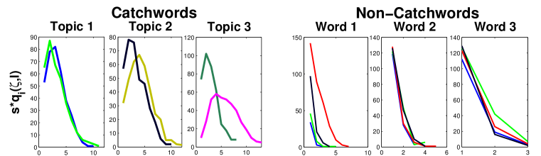
Figure 1: Plot of $q_{i}(\zeta,l)$ for some random catchwords (left) and non-catchwords (right). Each of three plots for catchword is for one topic ($l$) with two random catchwords ($i$) for each topic and each plot on right is for one non-catchword ($i$) with curves for multiple topics ($l$).

4.2 Empirical Results

4.2.1 Topic Recovery on Semi-Synthetic Data

Semi-synthetic Data: Following [5], we generate semi-synthetic corpora from LDA model trained by MCMC, to ensure that the synthetic corpora retain the characteristics of real data. Gibbs sampling is run for 1000 iterations on all the four datasets and the final word-topic distribution is used to generate varying number of synthetic documents with document-topic distribution drawn from a symmetric Dirichlet with hyper-parameter 0.01. For NIPS, NYT and Pubmed we use $k=50$ topics, for 20NewsGroup $k=20$, and mean document lengths of 1000, 300, 100 and 200 respectively. Note that the synthetic data is not guaranteed to satisfy dominant topic assumption for every document (on average about 80% documents satisfy the assumption for value of $(\alpha,\beta)$ tested in Section 4.1)

Topic Recovery: We learn the word-topic distributions ($\hat{M}$) for the semi-synthetic corpora using TSVD and the Recover algorithms of [5]. Given these learned topic distributions and the original data-generating distributions ($M$), we align the topics of $M$ and $\hat{M}$ by bipartite matching and rearrange the columns of $\hat{M}$ in accordance to the matching with $M$. Topic recovery is measured by the average of the $l_{1}$ error across topics (called reconstruction error [5]), $\Delta(M,\hat{M})$, defined as: $\Delta(M,\hat{M})=\frac{1}{k}\sum_{l=1}^{k}\sum_{i=1}^{d}|M_{il}-\hat{M}_{il}|$.

We report reconstruction error in Table 2 for TSVD and the Recover algorithms, Recover-L2 and Recover-KL. TSVD has smaller error on most datasets than the Recover-KL algorithm. We observed performance of TSVD to be always better than Recover-L2. Best performance is observed on NIPS which has largest mean document length, indicating that larger $m$ leads to better recovery. Results on 20NG are slightly worse than Recover-KL for small sample size (though better than Recover-L2), but the difference is small. While the values in Table 2 are averaged values, Figure 2 shows that TSVD algorithm achieves much better topic recovery (27% improvement in $l_{1}$ error over Recover-KL) for majority of the topics ($>$90%) on most datasets.

Corpus	Documents	Recover-L2	Recover-KL	TSVD	% Improvement
NIPS	40,000	0.342	0.308	0.115	62.7%
	50,000	0.346	0.308	0.145	52.9%
	60,000	0.346	0.311	0.131	57.9%
Pubmed	40,000	0.388	0.332	0.288	13.3%
	50,000	0.378	0.326	0.280	14.1%
	60,000	0.372	0.328	0.284	13.4%
20NG	40,000	0.126	0.120	0.124	-3.3%
	50,000	0.118	0.114	0.113	0.9%
	60,000	0.114	0.110	0.106	3.6%
NYT	40,000	0.214	0.208	0.195	6.3%
	50,000	0.211	0.206	0.185	10.2%
	60,000	0.205	0.200	0.194	3.0%

Table 2: L1 reconstruction error on various semi-synthetic datasets. Last column is percent improvement over Recover-KL (best performing Recover algorithm).

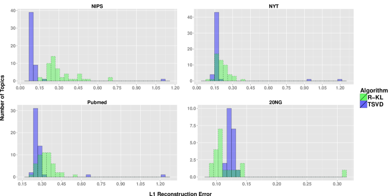
Figure 2: Histogram of $l_{1}$ error across topics for 40,000 synthetic documents. TSVD (blue, solid border) gets better recovery on most topics ($>90\%$) for most datasets (leaving small number of outliers) than Recover-KL (green, dashed border).

4.2.2 Topic Recovery on Real Data

Perplexity:

A standard quantitative measure used to compare topic models and inference algorithms is perplexity [2]. Perplexity of a set of $D$ test documents, where each document $j$ consists of $m_{j}$ words, denoted by $\textbf{w}_{j}$, is defined as: $perp(D_{test})=exp\left\{-\frac{\sum_{j=1}^{D}\log p(\textbf{w}_{j})}{\sum_{j=1}^{D}m_{j}}\right\}$. To evaluate perplexity on real data, the held-out sets consist of 350 documents for NIPS, 10000 documents for NYT and Pubmed, and 6780 documents for 20NewsGroup. Table 3 shows the results of perplexity on the 4 datasets. TSVD gives comparable perplexity with Recover-KL, results being slightly better on NYT and 20NewsGroup which are larger datasets with moderately high mean document lengths.

Topic Coherence:

[11] proposed Topic Coherence as a measure of semantic quality of the learned topics by approximating user experience of topic quality on top $d_{0}$ words of a topic. Topic coherence is defined as $TC(d_{0})=\sum_{i\leq d_{0}}\sum_{j<i}\log\frac{D(w_{i},w_{j})+e}{D(w_{j})}$, where $D(w)$ is the document frequency of a word $w$, $D(w_{i},w_{j})$ is the document frequency of $w_{i}$ and $w_{j}$ together, and $e$ is a small constant. We evaluate TC for the top 5 words of the recovered topic distributions and report the average and standard deviation across topics. TSVD gives comparable results on Topic Coherence (see Table 3).

Topics on Real Data:

Table LABEL:tab:topics shows the top 5 words of all 50 matched pair of topics on NYT dataset for TSVD, Recover-KL and Gibbs sampling. Most of the topics recovered by TSVD are more closer to Gibbs sampling topics. Indeed, the total average $l_{1}$ error with topics from Gibbs sampling for topics from TSVD is 0.034, whereas for Recover-KL it is 0.047 (on the NYT dataset).

Corpus	Perplexity			Topic Coherence
	R-KL	R-L2	TSVD	R-KL	R-L2	TSVD
NIPS	754	749	835	-86.4 $\pm\;$24.5	-88.6 $\pm\;$22.7	-65.2 $\pm\;$29.4
NYT	1579	1685	1555	-105.2 $\pm\;$25.0	-102.1 $\pm\;$28.2	-107.6 $\pm\;$25.7
Pubmed	1188	1203	1307	-94.0 $\pm\;$22.5	-94.4 $\pm\;$22.5	-84.5 $\pm\;$28.7
20NG	2431	2565	2390	-93.7 $\pm\;$13.6	-89.4 $\pm\;$20.7	-90.4 $\pm\;$27.0

Table 3: Perplexity and Topic Coherence. R-KL is Recover-KL, R-L2 is Recover-L2. Standard deviation for topic coherence across topics is also shown.

Summary: We evaluated the proposed algorithm, TSVD, rigorously on multiple datasets with respect to the state of the art (Recover), following the evaluation methodology of [5]. In Table 2 we show that the L1 reconstruction error for the new algorithm is small and on average 19.6% better than the best results of the Recover algorithms [5]. We also demonstrate that on real datasets the algorithm achieves comparable perplexity and topic coherence to Recover (Table 3. Moreover, we show on multiple real datasets that the algorithm assumptions are well justified in practice.

Conclusion

Real world corpora often exhibits the property that in every document there is one topic dominantly present. A standard SVD based procedure will not be able to detect these topics, however TSVD, a thresholded SVD based procedure, as suggested in this paper, discovers these topics. While SVD is time-consuming, there have been a host of recent sampling-based approaches which make SVD easier to apply to massive corpora which may be distributed among many servers. We believe that apart from topic recovery, thresholded SVD can be applied even more broadly to similar problems, such as matrix factorization, and will be the basis for future research.

Table 4: Top 5 words of matched topic pairs for TSVD, Recover-KL and Gibbs sampling. Catchwords and anchor words in top 5 words are highlighted for TSVD and Recover-KL

TSVD	Recover-KL	Gibbs
zzz_elian zzz_miami boy father zzz_cuba	zzz_elian boy zzz_miami father family	zzz_elian zzz_miami boy father zzz_cuba
cup minutes add tablespoon oil	cup minutes tablespoon add oil	cup minutes add tablespoon oil
game team yard zzz_ram season	game team season play zzz_ram	team season game coach zzz_nfl
book find british sales retailer	book find school woman women	book find woman british school
run inning hit season game	run season game inning hit	run season game hit inning
church zzz_god religious jewish christian	pope church book jewish religious	religious church jewish jew zzz_god
patient drug doctor cancer medical	patient drug doctor percent found	patient doctor drug medical cancer
music song album musical band	black reporter zzz_new_york zzz_black show	music song album band musical
computer software system zzz_microsoft company	web www site cookie cookies	computer system software technology mail
house dog water hair look	room show look home house	room look water house hand
zzz_china trade zzz_united_states nuclear official	zzz_china zzz_taiwan government trade zzz_party	zzz_china zzz_united_states zzz_u_s zzz_clinton zzz_american
zzz_russian war rebel troop military	zzz_russian zzz_russia war zzz_vladimir_putin rebel	war military zzz_russian soldier troop
officer police case lawyer trial	zzz_ray_lewis police case officer death	police officer official case investigation
car driver wheel race vehicles	car driver truck system model	car driver truck vehicle wheel
show network zzz_abc zzz_nbc viewer	con zzz_mexico son federal mayor	show television network series zzz_abc
com question information zzz_eastern sport	com information question zzz_eastern sport	com information daily question zzz_eastern
book author writer com reader	zzz_john_rocker player team right braves	book word writer author wrote
zzz_al_gore zzz_bill_bradley campaign president democratic	zzz_al_gore zzz_bill_bradley campaign president percent	zzz_al_gore campaign zzz_bill_bradley president democratic
actor film play movie character	goal play team season game	film movie award actor zzz_oscar
school student teacher district program	school student program million children	school student teacher program children
tax taxes cut billion plan	zzz_governor_bush tax campaign taxes plan	tax plan billion million cut
percent stock market fund investor	million percent tax bond fund	stock market percent fund investor
team player season coach zzz_nfl	team season player coach zzz_cowboy	team player season coach league
family home friend room school	look gun game point shot	family home father son friend
primary zzz_mccain voter zzz_john_mccain zzz_bush	zzz_john_mccain zzz_george_bush campaign republican voter	zzz_john_mccain zzz_george_bush campaign zzz_bush zzz_mccain
zzz_microsoft court company case law	zzz_microsoft company computer system software	zzz_microsoft company window antitrust government
company million percent shares billion	million company stock percent shares	company million companies business market
site web sites com www	web site zzz_internet company com	web site zzz_internet online sites
scientist human cell study researcher	dog quick jump altered food	plant human food product scientist
baby mom percent home family	mate women bird film idea	women look com need telegram
point game half shot team	point game team season zzz_laker	game point team play season
zzz_russia zzz_vladimir_putin zzz_russian zzz_boris_yeltsin zzz_moscow	zzz_clinton government zzz_pakistan zzz_india zzz_united_states	government political election zzz_vladimir_putin zzz_russia
com zzz_canada www fax information	chocolate food wine flavor buy	www com hotel room tour
room restaurant building fish painting	zzz_kosovo police zzz_serb war official	building town area resident million
loved family show friend play	film show movie music book	film movie character play director
prices percent worker oil price	percent stock market economy prices	percent prices economy market oil
million test shares air president	air wind snow shower weather	water snow weather air scientist
zzz_clinton flag official federal zzz_white_house	zzz_bradley zzz_al_gore campaign zzz_gore zzz_clinton	zzz_clinton president gay mayor zzz_rudolph_giuliani
files article computer art ball	show film country right women	art artist painting museum show
con percent zzz_mexico federal official	official zzz_iraq government zzz_united_states oil	zzz_mexico drug government zzz_united_states mexican
involving book film case right	test women study student found	plane flight passenger pilot zzz_boeing
zzz_internet companies company business customer	company companies deal zzz_internet zzz_time_warner	media zzz_time_warner television newspaper cable
zzz_internet companies company business customer	newspaper zzz_chronicle zzz_examiner zzz_hearst million	million money worker company pay
goal play games king game	zzz_tiger_wood shot tournament tour player	zzz_tiger_wood tour tournament shot player
zzz_american zzz_united_states zzz_nato camp war	zzz_israel zzz_lebanon peace zzz_syria israeli	zzz_israel peace palestinian talk israeli
team season game player play	team game point season player	race won win fight team
reporter zzz_earl_caldwell zzz_black black look	corp group list oil meeting	black white zzz_black hispanic reporter
campaign zzz_republican republican zzz_party primary	zzz_bush zzz_mccain campaign republican voter	gun bill law zzz_congress legislation
zzz_bush zzz_mccain campaign primary republican	flag black zzz_confederate right group	flag zzz_confederate zzz_south_carolina black zzz_south
zzz_john_mccain campaign zzz_george_bush zzz_bush republican	official government case officer security	court law case lawyer right

Table 4: Top 5 words of matched topic pairs for TSVD, Recover-KL and Gibbs sampling. Catchwords and anchor words in top 5 words are highlighted for TSVD and Recover-KL

Appendix A Line of Proof

We describe the Lemmas we prove to establish the result. The detailed proofs are in the Section B.

A.1 General Facts

We start with a consequence of the no-local-minimum assumption. We use that assumption solely through this Lemma.

Lemma A.1

Let $p_{i}(\zeta,l)$ be as in (6). If for some $\zeta_{0}\in\{0,1,\ldots,m\}$ and $\nu\geq 0$, $\sum_{\zeta\geq\zeta_{0}}p_{i}(\zeta,l)\geq\nu$ and also $\sum_{\zeta\leq\zeta_{0}}p_{i}(\zeta,l)\geq\nu$ then, $p_{i}(\zeta_{0},l)\geq\frac{\nu}{m}$.

Next, we state a technical Lemma which is used repeatedly. It states that for every $i,\zeta,l$, the empirical probability that $A_{ij}=\zeta/m$ is close to the true probability. Unsurprisingly, we prove it using H-C. But we will state a consequence in the form we need in the sequel.

Lemma A.2

Let $p_{i}(\zeta,l)$ and $q_{i}(\zeta,l)$ be as in (6) and (7). We have

$$\forall i,l,\zeta:\text{Prob}\left(\left|p_{i}(\zeta,l)-q_{i}(\zeta,l)\right|\geq\frac{\varepsilon}{2}\sqrt{w_{0}}\sqrt{p_{i}(\zeta,l)}+\frac{\varepsilon^{2}w_{0}}{2}\right)\quad\leq\;2\exp(-\varepsilon^{2}sw_{0}/8).$$

From this it follows that with probability at least $1-2\exp(-\varepsilon^{2}w_{0}s/8)$,

$$\frac{1}{2}q_{i}(\zeta,l)-\varepsilon^{2}w_{0}\quad\leq\;p_{i}(\zeta,l)\quad\leq\;2q_{i}(\zeta,l)+2\varepsilon^{2}w_{0}.$$

A.1.1 Properties of Thresholding

Say that a threshold $\zeta_{i}$ “splits” $T_{l}^{(2)}$ if $T_{l}^{(2)}$ has a significant number of $j$ with $A_{ij}>\zeta_{i}/m$ and also a significant number of $j$ with $A_{ij}\leq\zeta_{i}/m$. Intuitively, it would be desirable if no threshold splits any $T_{l}$, so that, in ${\bf B}$, for each $i,l$, either most $j\in T_{l}^{(2)}$ have $B_{ij}=0$ or most $j\in T_{l}^{(2)}$ have $B_{ij}=\sqrt{\zeta_{i}}$. We now prove that this is indeed the case with proper bounds. We henceforth refer to the conclusion of the Lemma below by the mnemonic “no threshold splits any $T_{l}$”.

Lemma A.3

(No Threshold Splits any $T_{l}$) For a fixed $i,l$, with probability at least $1-2\exp(-\varepsilon^{2}w_{0}s/8)$, the following holds:

$$\text{Min}\;\left(\text{Prob}(A^{(2)}_{ij}\leq\frac{\zeta_{i}}{m}\;;j\in T_{l}^{(2)}),\quad\text{Prob}(A^{(2)}_{ij}>\frac{\zeta_{i}}{m}\;;j\in T_{l}^{(2)})\right)\quad\leq 4m\varepsilon w_{0}.$$

Let $\mu$ be a $d\times s$ matrix whose columns are given by

$$\forall j\in T_{l}^{(2)}\;,\;\mu_{.,j}=E(B_{.,j}\;|\;j\in T_{l}).$$

$\mu$ ’s columns corresponding to all $j\in T_{l}$ are the same. The entries of the matrix $\mu$ are fixed (real numbers) once we have ${\bf A}^{(1)}$ (and the thresholds $\zeta_{i}$ are determined). Note: We have “integrated out $W$”, i.e.,

$$\mu_{ij}=\int_{W_{\cdot,j}}\text{Prob}(W_{.,j}|j\in T_{l})E(B_{ij}|W_{.,j}).$$

(So, think of $W_{\cdot,j}$ for ${\bf A}^{(1)}$ ’s columns being picked first from which $\zeta_{i}$ is calculated. $W_{\cdot,j}$ for columns of ${\bf A}^{(2)}$ are not yet picked until the $\zeta_{i}$ are determined.) But $\mu_{ij}$ are random variables before we fix ${\bf A}^{(1)}$. The following Lemma is a direct consequence of “no threshold splits any $T_{l}$”.

Lemma A.4

Let $\zeta_{i}^{\prime}=\text{Max}(\zeta_{i},8\ln(20/\varepsilon w_{0}))$. With probability at least $1-4kd\exp(-\varepsilon^{2}sw_{0}/8)$ (over the choice of ${\bf A}^{(1)}$):

$$\forall l,\forall j\in T_{l},\forall i: \mu_{ij}\leq\varepsilon_{l}\sqrt{\zeta_{i}^{\prime}}\text{ OR }\mu_{ij}\geq\sqrt{\zeta_{i}^{\prime}}(1-\varepsilon_{l})$$

$$\forall l,\forall i, \text{Var}(B_{ij})\leq 2\varepsilon_{l}\zeta_{i}^{\prime},$$ (10)

where, $\varepsilon_{l}=4m\varepsilon w_{0}/w_{l}$.

So far, we have proved that for every $i$, the threshold does not split any $T_{l}$. But this is not sufficient in itself to be able to cluster (and hence identify the $T_{l}$), since, for example, this alone does not rule out the extreme cases that for most $j$ in every $T_{l}$, $A_{ij}^{(2)}$ is above the threshold (whence $\mu_{ij}\geq(1-\varepsilon_{l})\sqrt{\zeta_{l}^{\prime}}$ for almost all $j$) or for most $j$ in no $T_{l}$ is $A_{ij}^{(2)}$ above the threshold, whence, $\mu_{ij}\leq\varepsilon_{l}\sqrt{\zeta_{i}^{\prime}}$ for almost all $j$. Both these extreme cases would make us loose all the information about $T_{l}$ due to thresholding; this scenario and milder versions of it have to be proven not to occur. We do this by considering how thresholds handle catchwords. Indeed we will show that for a catchword $i\in S_{l}$, a $j\in T_{l}$ has $A_{ij}^{(2)}$ above the threshold and a $j\notin T_{l}$ has $A_{ij}^{(2)}$ below the threshold. Both statements will only hold with high probability, of course and using this, we prove that $\mu_{.,j}$ and $\mu_{.,j^{\prime}}$ are not too close for $j,j^{\prime}$ in different $T_{l}$ ’s. For this, we need the following Lemmas.

Lemma A.5

For $i\in S_{l}$, and $l^{\prime}\not=l$, we have with $\eta_{i}=\big{\lfloor}\;M_{il}(\alpha+\beta+\rho)m/2\;\big{\rfloor}$,

$$\text{Prob}(A_{ij}\leq\eta_{i}/m\;|\;j\in T_{l})\leq\varepsilon w_{0}/20,\;\;\text{Prob}(A_{ij}\geq\eta_{i}/m\;|\;j\in T_{l^{\prime}})\leq\varepsilon w_{0}/20.$$

Lemma A.6

With probability at least $1-8mdk\exp(-\varepsilon^{2}w_{0}s/8)$, we have

$$\hbox{ for }j\in T_{l},j^{\prime}\notin T_{l},\;|\mu_{\cdot,j}-\mu_{\cdot,j^{\prime}}|^{2}\geq\frac{2}{9}\alpha p_{0}m.$$

A.1.2 Proximity

Next, we wish to show that clustering as in TSVD identifies the dominant topics correctly for most documents, i.e., that $R_{l}\approx T_{l}$ for all $l$. For this, we will use a theorem from [9] [see also [10]] which in this context says:

Theorem A.7

If all but a $f$ fraction of the the $B_{\cdot,j}$ satisfy the “proximity condition”, then TSVD identifies the dominant topic in all but $c_{1}f$ fraction of the documents correctly after polynomial number of iterations.

To describe the proximity condition, first let $\sigma$ be the maximum over all directions $v$ of the square root of the mean-squared distance of $B_{.,j}$ to $\mu_{.,j}$, i.e.,

$$\sigma^{2}=\text{Max}_{\|v\|=1}\frac{1}{s}|v^{T}({\bf B}-\mu)|^{2}=\frac{1}{s}\|{\bf B}-\mu\|^{2}.$$

The parameter $\sigma$ should remind the reader of standard deviation, which is indeed what this is, since $E({{\bf B}}|T_{1},T_{2},\ldots,T_{l})=\mu$. Our random variables $B_{.,j}$ being $d-$ dimensional vectors, we take the maximum standard deviation in any direction.

• ${\bf B}$ is said to satisfy the proximity condition with respect to $\mu$, if for each $l$ and each $j\in T_{l}$ and and each $l^{\prime}\not=l$ and $j^{\prime}\in T_{l^{\prime}}$, the projection of $B_{.,j}$ onto the line joining $\mu_{.,j}$ and $\mu_{.,j^{\prime}}$ is closer to $\mu_{.,j}$ by at least

  $$\Delta=\frac{c_{0}k}{\sqrt{w_{0}}}\sigma,$$

  than it is to $\mu_{.,j^{\prime}}$. [Here, $c_{0}$ is a constant.]

To prove proximity, we need to bound $\sigma$. This will be the task of the subsection B.1 which relies heavily on Random Matrix Theory.

Appendix B Proofs of Correctness

We start by recalling the Höffding-Chernoff (H-C) inequality in the form we use it.

Lemma B.1

Höffding-Chernoff If $X$ is the average of $r$ independent random variables with values in $[0,1]$ and $E(X)=\mu$, then, for an $t>0$,

$$\text{Prob}(X\geq\mu+t)\leq\exp\left(-\frac{t^{2}r}{2(\mu+t)}\right)\;;\;\text{Prob}(X\leq\mu-t)\leq\exp\left(-\frac{t^{2}r}{2\mu}\right).$$

• (of Lemma A.1) Abbreviate $p_{i}(\cdot,l)$ by $f(\cdot)$. We claim that either (i) $f(\zeta)\geq f(\zeta-1)\forall 1\leq\zeta\leq\zeta_{0}$ or (ii) $f(\zeta+1)\leq f(\zeta)\forall m-1\geq\zeta\geq\zeta_{0}.$ To see this, note that if both (i) and (ii) fail, we have $\zeta_{1}\leq\zeta_{0}$ and $\zeta_{2}\geq\zeta_{0}$ with $f(\zeta_{1})-f(\zeta_{1}-1)<0<f(\zeta_{2}+1)-f(\zeta_{2})$. But then there has to be a local minimum of $f$ between $\zeta_{1}$ and $\zeta_{2}$. If (i) holds, clearly, $f(\zeta_{0})\geq f(\zeta)\forall\zeta<\zeta_{0}$ and so the lemma follows. So, also if (ii) holds.

• (of Lemma A.2) Note that $q_{i}(\zeta,l)=\frac{1}{s}\left|\{j\in T_{l}:A_{ij}=\zeta/m\}\right|=\frac{1}{s}\sum_{j=1}^{s}X_{j},$ where, $X_{j}$ is the indicator variable of $A_{ij}=\zeta/m\;\wedge\;j\in T_{l}$. $\frac{1}{s}\sum_{j}E(X_{j})=p_{i}(\zeta,l)$ and we apply H-C with $t=\frac{1}{2}\varepsilon\sqrt{w_{0}}\sqrt{p_{i}(\zeta,l)}+\frac{1}{2}\varepsilon^{2}w_{0}$ and $\mu=p_{i}(\zeta,l)$. We have $\frac{t^{2}}{\mu+t}\geq\varepsilon^{2}w_{0}/4$, as is easily seen by calculating the roots of the quadratic $t^{2}-\frac{1}{4}t\varepsilon^{2}w_{0}-\frac{1}{4}\varepsilon^{2}w_{0}\mu=0$. Thus we get the claimed for $T_{l}$. Note that the same proof applies for $T_{l}^{(1)}$ as well as $T_{l}^{(2)}$.

  To prove the second assertion, let $a=q_{i}(\zeta,l)$ and $b=\sqrt{p_{i}(\zeta,l)}$, then, $b$ satisfies the quadratic inequalities:

  $$b^{2}-\frac{1}{2}\varepsilon\sqrt{w_{0}}b-(a+\frac{1}{2}\varepsilon^{2}w_{0})\leq 0\;;\;b^{2}+\frac{1}{2}\varepsilon\sqrt{w_{0}}b-(a-\frac{1}{2}\varepsilon^{2}w_{0})\geq 0.$$

  By bounding the roots of these quadratics, it is easy to see the second assertion after some calculation.

• (of Lemma A.3) Note that $\zeta_{i}$ is a random variable which depends only on $A^{(1)}$. So, for $j\in T_{l}^{(2)}$, $A_{ij}$ are independent of $\zeta_{i}$. Now, if

  $$\text{Prob}(A_{ij}\leq\frac{\zeta_{i}}{m}\;;j\in T_{l}^{(2)})>4m\varepsilon w_{0}\;\text{ and }\text{Prob}(A_{ij}>\frac{\zeta_{i}}{m}\;;j\in T_{l}^{(2)})>4m\varepsilon w_{0},$$

  by Lemma (A.1), we have

  $$\text{Prob}(A_{ij}=\frac{\zeta_{i}}{m};j\in T_{l}^{(2)})>4\varepsilon w_{0}.$$

  Since $\text{Prob}(A_{ij}=\zeta/m;j\in T_{l}^{(1)})=\text{Prob}(A_{ij}=\zeta/m;j\in T_{l}^{(2)})$ for all $\zeta$, we also have

  $$\text{Prob}(A_{ij}=\frac{\zeta_{i}}{m};j\in T_{l}^{(1)})=p_{i}(\zeta_{i},l)>4\varepsilon w_{0}.$$ (11)

  Pay a failure probability of $2\exp(-\varepsilon^{2}sw_{0}/8)$ and assume the conclusion of Lemma (A.2) and we have:

  $$\frac{1}{s}\left|\{j\in T_{l}^{(1)}:A_{ij}=\frac{\zeta_{i}}{m}\}\right|=q_{i}(\zeta_{i},l)\geq p_{i}(\zeta_{i},l)-\frac{\varepsilon}{2}\sqrt{w_{0}p_{i}(\zeta_{i},l)}-\frac{\varepsilon^{2}}{2}w_{0}.$$

  Now, it is easy to see that $p_{i}(\zeta,l)-\frac{\varepsilon}{2}\sqrt{w_{0}p_{i}(\zeta,l)}$ increases as $p_{i}(\zeta,l)$ increases subject to (11). So,

  $$p_{i}(\zeta,l)-\frac{\varepsilon}{2}\sqrt{w_{0}p_{i}(\zeta,l)}-\frac{\varepsilon^{2}}{2}w_{0}>(4\varepsilon-\varepsilon^{3/2}-\frac{1}{2}\varepsilon^{2})w_{0}\geq 3\varepsilon w_{0},$$

  contradicting the definition of $\zeta_{i}$ in the algorithm. This completes the proof of the Lemma.

• (of Lemma A.4): After paying a failure probability of $4kd\exp(-\varepsilon^{2}sw_{0}/8)$, assume no threshold splits any $T_{l}$. [The factors of $k$ and $d$ come in because we are taking the union bound over all words and all topics.] Then,

  $$\text{Prob}(A_{ij}^{(2)}\leq\frac{\zeta_{i}}{m}\;|\;j\in T_{l}^{(2)}) =\sum_{\zeta=0}^{\zeta_{i}}p_{i}(\zeta,l)/\text{Prob}(j\in T_{l})\leq 4m\varepsilon\frac{w_{0}}{w_{l}}$$

  $$\text{ or }\text{Prob}(A_{ij}^{(2)}>\frac{\zeta_{i}}{m}\;|\;j\in T_{l}^{(2)}) =\sum_{\zeta=\zeta_{i}+1}^{m}p_{i}(\zeta,l)/\text{Prob}(j\in T_{l})\leq 4m\varepsilon\frac{w_{0}}{w_{l}}.$$

  Wlg, assume that $\text{Prob}(A_{ij}\leq\zeta_{i}/m\;|\;j\in T_{l})\leq\varepsilon_{l}$. Then, with probability, at least $1-\varepsilon_{l}$, $A_{ij}^{(2)}>\zeta_{i}/m$. Now, either $\zeta_{i}<8\ln(20/\varepsilon w_{0})$ and all $B_{ij},j\in T_{l}$ are zero and then $\mu_{ij}=0$, or $\zeta_{i}\geq 8\ln(20/\varepsilon w_{0})$, whence, $E(B_{ij}|j\in T_{l})\in[(1-\varepsilon_{l})\sqrt{\zeta_{i}^{\prime}},\sqrt{\zeta_{i}^{\prime}}]$. So, $\mu_{ij}\geq(1-\varepsilon_{l})\sqrt{\zeta^{\prime}_{i}}$ and $\text{Prob}(B_{ij}=0)\leq\varepsilon_{l}$. So,

  $$\text{Var}(B_{ij}^{2}|j\in T_{l})\leq(\sqrt{\zeta_{i}^{\prime}}-(1-\varepsilon_{l})\sqrt{\zeta_{i}^{\prime}})^{2}\text{Prob}(B_{ij}=\sqrt{\zeta_{i}^{\prime}}|j\in T_{l})+(\sqrt{\zeta_{i}^{\prime}}-0)^{2}\text{Prob}(B_{ij}=0|j\in T_{l})\leq 2\varepsilon_{l}\zeta_{i}^{\prime}.$$

  This proves the lemma in this case. The other case is symmetric.

• (of Lemma A.5) Recall that $P_{ij}=\sum_{l}M_{il}W_{lj}$ is the probability of word $i$ in document $j$ conditioned on ${\bf W}$. Fix an $i\in S_{l}$. From the dominant topic assumption,

  $$\forall j\in T_{l},P_{ij}=\sum_{l_{1}}M_{il_{1}}W_{l_{1},j}\geq M_{il}W_{lj}\geq M_{il}\alpha.$$ (12)

  The $P_{ij}$ are themselves random variables. Note that (12) holds with probability 1. From Catchword assumption and (1), we get that

  $$M_{il}\alpha-(\eta_{i}/m)\geq M_{il}\alpha-M_{il}((\alpha+\beta+\rho)/2)\geq M_{il}\alpha\delta/2.$$

  Now, we will apply H-C with $\mu-t=\eta_{i}/m$ and $\mu\geq M_{il}\alpha$ for the $m$ independent words in a document. By Calculus, the probability bound from H-C of $\exp(-t^{2}w_{l}s/2\mu)=\exp(-(\mu-(\eta_{i}/m))/2\mu)$ is highest subject to the constraints $\mu\geq M_{il}\alpha;\eta_{i}\leq mM_{il}(\alpha+\beta+\rho)/2$, when $\mu=M_{il}\alpha$ and $\eta_{i}=mM_{il}(\alpha+\beta+\rho)/2$, whence, we get

  $$\text{Prob}(A_{ij}\leq\eta_{i}/m\;|\;j\in T_{l})\leq\exp(-M_{il}\alpha\delta^{2}m/8)\leq\varepsilon w_{0}/20,$$

  using (5). Now, we prove the second assertion of the Lemma.

  $$\forall j\in T_{l^{\prime}},l^{\prime}\not=l,\sum_{l_{1}}M_{il_{1}}W_{l_{1},j}=M_{il}W_{lj}+\sum_{l_{1}\not=l}M_{il_{1}}W_{l_{1},j}$$

  $$\leq M_{il}W_{lj}+\left(\text{Max}_{l_{1}\not=l}M_{il_{1}}\right)(1-W_{lj})$$

  $$\leq M_{il}(\beta+\rho).$$ (13)

  $$\frac{\eta_{i}}{m}-M_{il}(\beta+\rho)\geq\frac{M_{il}(\alpha+\beta+\rho)}{2}-M_{il}(\beta+\rho)-\frac{1}{m}\geq\frac{3M_{il}\alpha\delta}{8},$$

  using (5) and (1). Applying the first inequality of Lemma (B.1) with $\mu+t=\eta_{i}/m$ and $\mu\leq M_{il}(\beta+\rho)$ and again using (5),

  $$\text{Prob}(A_{ij}\geq\eta_{i}/m\;|\;j\in T_{l^{\prime}})\leq\exp\left(-9M_{il}\alpha\delta^{2}m/64\right)\leq\varepsilon w_{0}/20.$$

Lemma B.2

For $i\in S_{l}$, $\text{Prob}(\zeta_{i}<\eta_{i})\leq 3mke^{-\varepsilon^{2}sw_{0}/8}$, with $\eta_{i}$ as defined in Lemma A.5.

• Fix attention on $i\in S_{l}$. After paying the failure probability of $3mke^{-\varepsilon^{2}sw_{0}/8}$, assume the conclusions of Lemma (A.2) hold for all $\zeta,l$. It suffices to show that

  $$\left|\{j:A_{ij}^{(1)}>\eta_{i}/m\}\right|\geq\frac{w_{0}s}{2}\;\;,\;\;\left|\{j:A_{ij}^{(1)}=\frac{\eta_{i}}{m}\}\right|<3w_{0}\varepsilon s,$$

  since, $\eta_{i}$ is an integer and $\zeta_{i}$ is the largest integer satisfying the inequalities. The first statement follows from first assertion of Lemma A.5. The second statement is slightly more complicated. Using both the first and second assertions of Lemma A.5, we get that for all $l^{\prime}$ (including $l^{\prime}=l$), we have

  $$\text{Prob}(A_{ij}=\eta_{i}/m|j\in T_{l^{\prime}}^{(1)})\leq\varepsilon w_{0}/20.$$

  $$\left|\{j\in T_{l^{\prime}}^{(1)}:A_{ij}=\eta_{i}/m\}\right|\leq\varepsilon w_{0}w_{l^{\prime}}s/20+\frac{\varepsilon}{2}\sqrt{w_{0}/w_{l^{\prime}}}\sqrt{\varepsilon w_{0}/20}w_{l^{\prime}}s+\frac{\varepsilon^{2}w_{0}w_{l^{\prime}}}{2}$$

  $$\leq\frac{\varepsilon w_{0}s}{8}\left(w_{l^{\prime}}+\sqrt{\varepsilon w_{l^{\prime}}}\right)+\frac{\varepsilon^{2}w_{0}s}{2}.$$

  Now, adding over all $l^{\prime}$ and using $\sum_{l^{\prime}}\sqrt{w_{l^{\prime}}}\leq\sqrt{k}\sqrt{\sum_{l^{\prime}}w_{l^{\prime}}}=\sqrt{k}$, we get

  $$\left|\{j:A_{ij}^{(1)}=\eta_{i}/m\}\right|\leq\varepsilon w_{o}s,$$

  since $\varepsilon\leq 1/k$.

Lemma B.3

Define $I_{l}=\{i\in S_{l}:\zeta_{i}\geq\eta_{i}\}$. With probability at least $1-8mdk\exp(-\varepsilon^{2}w_{0}s/8)$, we have for all $l$,

$$\sum_{i\in I_{l}}\zeta_{i}^{\prime}\geq m\alpha p_{0}/2.$$

• After paying the failure probability, we assume the conclusion of Lemma A.2 holds for all $i,\zeta,l$. Now, by Lemma B.2, we have (with ${\bf 1}$ denoting the indicator function)

  $$E\left(\sum_{i\in S_{l}}M_{il}{\bf 1}(\zeta_{i}<\eta_{i})\right)\leq 3mk\exp(-\varepsilon^{2}sw_{0}/8)\sum_{i\in S_{l}}M_{il},$$

  which using Markov inequality implies that with probability at least $1-6mk\exp(-\varepsilon^{2}sw_{0}/8)$,

  $$\sum_{i\in I_{l}}M_{il}\geq\frac{1}{2}\sum_{i\in S_{l}}M_{il}\geq p_{0}/2,$$ (14)

  using (4). Note that by (5), no catchword has $\zeta_{i}^{\prime}$ set to zero. So,

  $$\sum_{i\in I_{l}}\zeta_{i}^{\prime}=\sum_{i\in I_{l}}\zeta_{i}\geq\sum_{i\in I_{l}}\eta_{i}\geq\sum_{I_{l}}mM_{il}\alpha/2\geq\alpha p_{0}m/2.$$

• (of Lemma A.6) For this proof, $i$ will denote an element of $I_{l}$. By Lemma A.5,

  $$\forall i\in I_{l},l^{\prime}\not=l,\text{Prob}(A_{ij}>\frac{\zeta_{i}}{m}|j\in T_{l^{\prime}}^{(1)})\leq\text{Prob}(A_{ij}>\eta_{i}/m|j\in T_{l^{\prime}}^{(1)})\leq\frac{\varepsilon w_{0}}{20}.$$ (15)

  This implies by Lemma A.2, for $l^{\prime}\not=l$,

  $$\left|\{j\in T_{l^{\prime}}^{(1)}:A_{ij}>\frac{\zeta_{i}}{m}\}\right|\leq w_{l^{\prime}}s\left(\frac{\varepsilon w_{0}}{20}+\varepsilon\sqrt{w_{0}/w_{l^{\prime}}}\sqrt{\varepsilon w_{0}}/4\right)+w_{0}\varepsilon^{2}s/2.$$ (16)

  Summing over all $l^{\prime}\not=l$, we get (using $\sum_{l^{\prime}}\sqrt{w_{l^{\prime}}}\leq\sqrt{\sum w_{l^{\prime}}}\sqrt{k}\leq 1/\sqrt{\varepsilon}$ by (9))

  $$\sum_{l^{\prime}\not=l}\left|\{j\in T_{l^{\prime}}^{(1)}:A_{ij}>\frac{\zeta_{i}}{m}\}\right|\leq\varepsilon w_{0}s.$$

  Now the definition of $\zeta_{i}$ in the algorithm implies that:

  $$\sum_{\zeta>\zeta_{i}}q_{i}(\zeta,l)=\left|\{j\in T_{l}^{(1)}:A_{ij}>\frac{\zeta_{i}}{m}\}\right|\geq\left(\frac{w_{0}}{2}-\varepsilon w_{0}\right)s\geq w_{0}s/4.$$

  So, by Lemma A.2,

  $$\text{Prob}(j\in T_{l};A_{ij}>\zeta_{i}/m)=\sum_{\zeta>\zeta_{i}}p_{i}(\zeta,l)\geq\frac{1}{2}\sum_{\zeta>\zeta_{i}}q_{i}(\zeta,l)-\varepsilon^{2}w_{0}m$$

  $$\geq\frac{w_{0}}{8}-\varepsilon^{2}w_{0}m\geq w_{0}/9,$$

  using (9). Next let $\tilde{p}=\text{Prob}(A_{ij}=\zeta_{i}/m;j\in T_{l})$. Since $|\{j\in T_{l}^{(1)}:A_{ij}=\zeta_{i}/m\}|\leq 3\varepsilon w_{0}s$, by the definition of $\zeta_{i}$ in the algorithm, we get by a similar argument

  $$\tilde{p}\leq 2q_{i}(\zeta_{i},l)+2\varepsilon^{2}w_{0}\leq 7\varepsilon w_{0}.$$ (17)

  Now, by Lemma A.1, we have

  $$\tilde{p}\geq\text{Min}\left(\frac{w_{0}}{9m}\;,\;\frac{1}{m}\text{Prob}(A_{ij}\leq\zeta_{i}/m;j\in T_{l}^{(2)})\right).$$

  By (9), $7\varepsilon w_{0}<w_{0}/9m$ and so we get:

  $$\text{Prob}(A_{ij}\leq\zeta_{i}/m;j\in T_{l}^{(2)})\leq 7\varepsilon mw_{0}.$$

  Noting that by (5), no catchword has $\zeta_{i}^{\prime}$ set to zero, $\text{Prob}(B_{ij}=0|j\in T_{l}^{(2)})\leq 7\varepsilon mw_{0}/w_{l}\leq 1/6$, by (9). This implies

  $$\mu_{ij}\geq\frac{5}{6}\sqrt{\zeta_{i}^{\prime}}.$$

  Now, by (15), we have for $j^{\prime}\notin T_{l}$,

  $$\mu_{ij^{\prime}}\leq\sqrt{\zeta_{i}^{\prime}}/6.$$

  So, we have

  $$\left|\mu_{\cdot,j}-\mu_{\cdot,j^{\prime}}\right|^{2}\geq\sum_{i\in I_{l}}(\mu_{ij}-\mu_{ij^{\prime}})^{2}\geq(4/9)\sum_{i\in I_{l}}\zeta_{i}^{\prime}.$$

  Now Lemma (B.3) implies the current Lemma.

B.1 Bounding the Spectral norm

Theorem B.4

Fix an $l$. For $j\in T_{l}$, let $R_{.,j}=B_{.,j}-\mu_{.,j}$. [The $R_{.,j},j\in T_{l}$ are vector-valued random variables which are independent, even conditioned on the partition $T_{1},T_{2},\ldots,T_{k}$.] With probability at least $1-10mdk\exp(-\varepsilon^{2}w_{0}s/8)$, we have $||R||^{2}\leq ckw_{0}\varepsilon sm^{2}.$ Thus,

$$||{\bf B}-\mu||^{2}\leq c\varepsilon w_{0}sm^{2}k^{2}.$$

We will apply Random Matrix Theory, in particular the following theorem, to prove Theorem B.4.

Theorem B.5

[15, Theorem 5.44] Suppose $R$ is a $d\times r$ matrix with columns $R_{\cdot,j}$ which are independent identical vector-valued random variables. Let $U=E(R_{\cdot,j}R_{\cdot,j}^{T})$ be the inertial matrix of $R_{\cdot,j}$. Suppose $|R_{\cdot,j}|\leq\nu$ always. Then, for any $t>0$, with probability at least $1-de^{-ct^{2}}$, we have

$$||R||\leq||U||^{1/2}\sqrt{r}+t\nu.$$

We need the following Lemma first.

Lemma B.6

With probability at least $1-\exp(-s\varepsilon w_{0}/3)$, we have

$$\zeta_{0}\leq 4m\lambda\;\;;\;\;\sum_{i}\zeta_{i}^{\prime}\leq 4km$$ (18)

• The probability of word $i$ in document $j$, is given by: $P_{ij}=\sum_{l}M_{il}W_{lj}\leq\lambda_{i}$ (where, $\lambda_{i}=\max_{l}M_{il}$). If $\lambda_{i}<\frac{1}{m}\ln(20/\varepsilon w_{0})$, then, $\text{Prob}(A_{ij}>(8/m)\ln(20/\varepsilon w_{0}))\leq\varepsilon w_{0}$ by H-C (since $A_{ij}$ is the average of $m$ i.i.d. trials). Let $X_{j}$ be the indicator function of $A_{ij}>(8/m)\ln(20/\varepsilon w_{0})$. $X_{j}$ are independent and so using H-C, we see that with probability at least $1-\exp(-\varepsilon w_{0}s/3)$, less than $w_{0}s/2$ of the $A_{ij}$ are greater $(8/m)\ln(20/\varepsilon w_{0})$, whence, $\zeta_{i}^{\prime}=0$. So we have (using the union bound over all words):

  $$\text{Prob}\left(\sum_{i:\lambda_{i}<(1/m)\ln(20/\varepsilon w_{0})}\zeta_{i}^{\prime}>0\right)\leq d\exp(-\varepsilon w_{0}s/3).$$

  If $\lambda_{i}\geq(1/m)\ln(20/\varepsilon w_{0})$, then

  $$\text{Prob}(A_{ij}>4\lambda_{i})\leq e^{-\lambda_{i}m}\leq\varepsilon w_{0}/2,$$

  which implies by the same $X_{j}$ kind of argument that with probability at least $1-\exp(-\varepsilon w_{0}s/4)$, for a fixed $i$, $\zeta_{i}\leq 4\lambda_{i}m$. Using the union bound over all words and adding all $i$, we get that with probability at least $1-2d\exp(-\varepsilon w_{0}s/4)$,

  $$\sum_{i}\zeta_{i}^{\prime}\leq 4m\sum_{i}\lambda_{i}\leq 4m\sum_{i,l}M_{il}\leq 4km.$$

  Now we prove the bound on $\zeta_{0}$. For each fixed $i,j$, we have $\text{Prob}(A_{ij}\geq 4\lambda)\leq e^{-m\lambda}\leq\varepsilon w_{0}$. Now, let $Y_{j}$ be the indicator variable of $A_{ij}\geq 4\lambda$. The $Y_{j},j=1,2,\ldots,s$ are independent (for each fixed $i$). So, $\text{Prob}(\zeta_{i}\geq 4m\lambda)\leq\text{Prob}(\sum_{j}Y_{j}\geq w_{0}s/2)\leq e^{-\varepsilon w_{o}s/3}$. Using an union bound over all words, we get that $\text{Prob}(\zeta_{0}>4m\lambda)\leq de^{-\varepsilon w_{0}/3}$ by H-C.

• (of Theorem B.4) First,

  $$||U||=\text{Max}_{|v|=1}E(v^{T}R_{\cdot,j})^{2}\leq E(|R_{\cdot,j}|^{2})\leq 2\varepsilon_{l}\sum_{i}\zeta_{i}^{\prime}\leq 8\varepsilon_{l}km,$$

  by Lemma (B.6) and Lemma (A.4). We can also take $\nu=2\sqrt{km}$ in Theorem B.5 and with $t=\sqrt{\varepsilon mw_{0}s}$, the first statement of the current theorem follows (noting $r=w_{l}s$). The second statement follows by just paying a factor of $k$ for the $k$ topics.

B.2 Proving Proximity

From Theorem (B.4), the $\sigma$ in definition A.1.2 is $\sqrt{c\varepsilon w_{0}m^{2}k^{2}}$. So, the $\Delta$ in definition A.1.2 is $cc_{0}\sqrt{\varepsilon}k^{2}m$. So it suffices to prove:

Lemma B.7

For $j\in T_{l}$ and $j^{\prime}\in T_{l^{\prime}},l^{\prime}\not=l$, let $\hat{B}_{.,j}$ be the projection of $B_{.,j}$ onto the line joining $\mu_{.,j}$ and $\mu_{.,j^{\prime}}$. The probability that $|\hat{B}_{.,j}-\mu_{.,j^{\prime}}|\leq|\hat{B}_{.,j}-\mu_{.,j}|+cc_{0}k^{2}\sqrt{\varepsilon}m$ is at most $c\varepsilon mw_{0}\sqrt{k}/\sqrt{\alpha p_{0}}$. Hence, with probability at least $1-cmdk\exp(-cw_{0}\varepsilon^{2}s)$, the number of $j$ for which $B_{.,j}$ does not satisfy the proximity condition is at most $c\varepsilon_{0}w_{0}\delta s/10c_{1}$.

• After paying the failure probability of $cmdk\exp(-w_{0}s\varepsilon^{2}/8)$, of Lemmas (B.6) and (A.6), assume that $\zeta_{0}\leq 4m\lambda$ , $|\mu_{.,j}-\mu_{.,j^{\prime}}|^{2}\geq 2\alpha mp_{0}/9$ and $\sum_{i}\zeta_{i}^{\prime}\leq 4km$.

  Let $X=(B_{\cdot,j}-\mu_{\cdot,j})\cdot(\mu_{\cdot,j^{\prime}}-\mu_{\cdot,j})$. $X$ is a random variable, whose expectation is 0 conditioned on $j\in T_{l}^{(2)}$.

  Since $\text{Prob}(B_{ij}=\sqrt{\zeta_{i}^{\prime}}|j\in T_{l})=\mu_{ij}/\sqrt{\zeta_{i}^{\prime}}$, we have:

  $$E|X| \leq E\sum_{i}|B_{ij}-\mu_{ij}|\;|\mu_{ij^{\prime}}-\mu_{ij}|$$

  $$=\sum_{i}\left[(\sqrt{\zeta_{i}^{\prime}}-\mu_{ij})\frac{\mu_{ij}}{\sqrt{\zeta_{i}^{\prime}}}+(1-\frac{\mu_{ij}}{\sqrt{\zeta_{i}^{\prime}}})\mu_{ij}\right]|\mu_{ij}-\mu_{ij^{\prime}}|$$

  $$\leq 2\varepsilon_{l}\sum_{i}\sqrt{\zeta_{i}^{\prime}}|\mu_{ij}-\mu_{ij^{\prime}}|\quad\text{ by Lemma \ref{define-R}}$$

  $$\leq 2\varepsilon_{l}\left(\sum_{i}\zeta_{i}^{\prime}\right)^{1/2}|\mu_{.,j}-\mu_{.,j^{\prime}}|\leq 4\varepsilon_{l}\sqrt{km}|\mu_{.,j}-\mu_{.,j^{\prime}}|.$$

  Now apply Markov inequality to get

  $$\text{Prob}(|X|\geq\frac{1}{8}|\mu_{.,j}-\mu_{.,j^{\prime}}|^{2})\leq 32\varepsilon_{l}\sqrt{km}/|\mu_{.,j}-\mu_{.,j^{\prime}}|\leq 80\varepsilon_{l}\sqrt{k/\alpha p_{0}}.$$

  If $|X|\leq|\mu_{.,j}-\mu_{.,j^{\prime}}|^{2}/8$, then, $|\hat{B}_{.,j}-\mu_{.,j^{\prime}}|\geq|\hat{B}_{.,j}-\mu_{.,j}|+3|\mu_{.,j}-\mu_{.,j^{\prime}}|/4\geq|\hat{B}_{.,j}-\mu_{.,j}|+cc_{0}k^{2}\sqrt{\varepsilon}m$, by (9). This proves the first assertion of the Lemma.

  The second statement of Lemma follows by applying H-C to the random variable $\sum_{j}Z_{j}/s$, where, $Z_{j}$ is the indicator random variable of $B_{.,j}$ not satisfying the proximity condition (and using (9).)

The last Lemma implies that the algorithm TSVD correctly identifies the dominant topic in all but at most $\varepsilon_{0}w_{0}/10$ fraction of the documents by Theorem (A.7).

Lemma B.8

With probability at least $1-\exp(-w_{0}s\varepsilon^{2}/8)$, TSVD correctly identifies the dominant topic in all but at most $\varepsilon_{0}w_{0}\delta/10$ fraction of documents in each $T_{l}$.

B.3 Identifying Catchwords

Recall the definition of $J_{l}$ from Step 5a of the algorithm. The two lemmas below are roughly converses of each other which prove roughly that $J_{l}$ consists of those $i$ for which $M_{il}$ is strictly higher than $M_{il^{\prime}}$. Using them, Lemma B.11 says that almost all the $\varepsilon_{0}w_{0}s/2$ documents found in Step 6 of the algorithm are $1-\delta$ pure for topic $l$.

Lemma B.9

Let $\nu=\gamma(1-2\delta)/(1+\delta)$. If $i\in J_{l}$, then for all $l^{\prime}\not=l$, $M_{il}\geq\nu M_{il^{\prime}}$ and $M_{il}\geq\frac{3}{m\delta^{2}}\ln(20/\varepsilon w_{0})$.

• It is easy to check that the assumptions (2) and (1)imply $\nu\geq 2$. Let $i\in J_{l}$. By the definition of $J_{l}$ in the algorithm, $g(i,l)\geq(4/m\delta^{2})\ln(20/\varepsilon w_{0}).$ Note that $P_{ij}\leq\text{Max}_{l_{1}}M_{il_{1}}$ for all $j$. So,

  $$\max_{l_{1}}M_{il_{1}}\geq\frac{3}{m\delta^{2}}\ln(20/\varepsilon w_{0}).$$ (19)

  If the Lemma is false, then, for $l^{\prime}$ attaining Max${}_{l_{1}\not=l}M_{il_{1}}$, we have $M_{il}<\nu M_{il^{\prime}}$. Recall $R_{l^{\prime}}$ defined in Step 4c of the algorithm. Let

  $$\hat{T}_{l^{\prime}}=R_{l^{\prime}}\cap\;(\text{ the set of $1-\delta$ pure documents in }T_{l^{\prime}}).$$

  Since all but $\varepsilon_{0}w_{0}s/10$ documents in $T_{l^{\prime}}$ belong to $R_{l^{\prime}}$, we have $|\hat{T}_{l^{\prime}}|\geq 0.9\varepsilon_{0}w_{0}s$. For $j\in\hat{T}_{l^{\prime}}$, $P_{ij}\geq M_{il^{\prime}}W_{l^{\prime}j}\geq(1-\delta)M_{il^{\prime}}$. So, $\text{Prob}(A_{ij}<M_{il^{\prime}}(1-2\delta))\leq\exp(-m\delta^{2}M_{il^{\prime}}/3)\leq\varepsilon w_{0}/4$ using (19). Thus the number of documents in $R_{l^{\prime}}$ for which $A_{ij}\geq M_{il^{\prime}}(1-2\delta)$ is at least $0.9\varepsilon_{0}w_{0}s-3\varepsilon w_{0}s\geq.6\varepsilon_{0}w_{0}s$. This implies that with probability at least $1-\exp(-c\varepsilon^{2}sw_{0})$, $g(i,l^{\prime})\geq M_{il^{\prime}}(1-2\delta)$.

  Now, for $j\in T_{l}$, $P_{ij}\leq\text{Max}(M_{il},M_{il^{\prime}})\leq\nu M_{il^{\prime}}$. So, $\text{Prob}(A_{ij}>M_{il^{\prime}}\nu(1+\delta))\leq\varepsilon w_{0}/4$, again using (19). At most $\varepsilon_{0}w_{0}s/10$ documents of other $T_{l_{1}}$, $l_{1}\not=l$ are in $R_{l}$ (by Lemma B.8). So, whp, $g(i,l)\leq M_{il^{\prime}}\nu(1+\delta)$ and so we have

  $$g(i,l)\leq\frac{\nu(1+\delta)}{1-2\delta}g(i,l^{\prime}),$$

  contradicting the definition of $J_{l}$. So, we must have that $M_{il}\geq\nu M_{il^{\prime}}$ for all $l^{\prime}\not=l$. The second assertion of the Lemma now follows from (19).

Lemma B.10

If $M_{il}\geq\text{Max}\left(\frac{5}{m\delta^{2}}\ln(20/\varepsilon w_{0}),\text{Max}_{l^{\prime}\not=l}\frac{1}{\rho}\;M_{il^{\prime}}\right)$, then, with probability at least $1-\exp(-c\varepsilon^{2}w_{0}s)$, we have that $i\in J_{l}$. So, $S_{l}\subseteq J_{l}$.

• Let $\hat{T}_{l}=R_{l}\cap$ (set of $1-\delta$ pure documents in $T_{l}$). For $j\in\hat{T}_{l}$, $P_{ij}\geq M_{il}(1-\delta)$ which implies that whp, (since $|\hat{T}_{l}|\geq 0.9\varepsilon_{0}s$, again by Lemma B.8)

  $$g(i,l)\geq M_{il}(1-2\delta)$$ (20)

  On the other hand, for $j\in T_{l^{\prime}}$ and for $l^{\prime}\not=l$, $i:M_{il^{\prime}}\leq\rho M_{il}$ (hypothesis of the Lemma), $P_{ij}\leq M_{il}W_{lj}+\rho M_{il}(1-W_{lj})\leq M_{il}(\beta+\rho)$. So whp,

  $$g(i,l^{\prime})\leq M_{il}(\beta+\rho)(1+\delta).$$ (21)

  From (20) and (21) and hypothesis of the Lemma, it follows that

  $$g(i,l)\geq\text{Max}\left(\frac{4}{m\delta^{2}}\ln(1/\varepsilon w_{0}),\frac{(1-2\delta)}{(1+\delta)(\beta+\rho)}\;g(i,l^{\prime})\right).$$

  So, $i\in J_{l}$ as claimed. It only remains to check that $i$ in $S_{l}$ satisfies the hypothesis of the Lemma which is obvious.

Lemma B.11

Let $\nu_{l}=\sum_{i\in J_{l}}M_{il}$ and let $L$ be the set of $\lfloor(s\varepsilon_{0}w_{0}/2)\rfloor$ $A_{.,j}$ ’s whose average is returned in Step 6 of the TSVD Algorithm as $\hat{M}_{.,l}$. With probability at least $1-c\exp(-c\varepsilon^{2}w_{0}s)$, we have:

$$\left|\frac{1}{|L|}\sum_{j\in L}(A_{.,j}-M_{.,l})\right|_{1}\leq O(\delta).$$ (22)

• The proof needs care since $J_{l}$ is itself a random set dependent on $A^{(2)}$. To understand the proof intuitively, if we pretend that there is no conditioning of $J_{l}$ on $A^{(2)}$, then, basically, our arguments in Lemma B.9 would yield this Lemma. However, we have to work harder to avoid conditioning effects. Define

  $$K_{l}=\{i:M_{il}\geq\nu M_{il^{\prime}}\forall l^{\prime}\not=l;M_{il}\geq(3/m\delta^{2})\ln(20/\varepsilon w_{0})\}.$$

  Note that $K_{l}$ is not a random set; it does not depend on $A$, just on $M$ which is fixed. Lemma B.9 proved that $J_{l}\subseteq K_{l}$. Since $\sum_{i}M_{il}=1$, we have $|K_{l}|\leq m\delta^{2}/3$. The probability bounds given here will be after conditioning on ${\bf W}$. [In other words, we prove statements of the form $\text{Prob}({\cal E}|{\bf W})\leq a$ which is (the usual) shorthand for: for each possible value $w$ of the matrix $W$, $\text{Prob}({\cal E}\;|\;{\bf W}=w)\leq a$.] This will be possible, since, even after fixing $W$, the $A_{.,j}$ are independent, though certainly not identically distributed now, since the $W_{.,j}$ may differ.

For $i\in K_{l}$, we have for all $j$, $P_{ij}=\sum_{l^{\prime}}M_{il^{\prime}}W_{l^{\prime}j}\leq M_{il}$, since, $M_{il^{\prime}}\leq M_{il}/\nu\leq M_{il}/2$ for $l^{\prime}\not=l$. For any $x\leq M_{il}$,

$$\text{Prob}(|A_{ij}^{(2)}-P_{ij}|\geq\delta M_{il}\;|\;W,P_{ij}=x)\leq 2\exp\left(-\frac{\delta^{2}M_{il}^{2}m}{2(1+\delta)x}\right)\leq 2\exp\left(-\frac{m\delta^{2}M_{il}}{3}\right).$$

Noting that $m\delta^{2}M_{il}\geq 3\ln(20/\varepsilon w_{0})$ for $i\in K_{l}$, we get

$$\text{Prob}(|A_{ij}^{(2)}-P_{ij}|\geq\delta M_{il}\;|\;W)\leq\varepsilon w_{0}/20.$$

Using the union bound over all $i\in K_{l}$ yields (for each $j\in[s]$),

$$\text{Prob}(\exists i\in K_{l}:|A_{ij}^{(2)}-P_{ij}|\geq\delta M_{il}\;|\;W)\leq\frac{m\delta^{2}\varepsilon w_{0}}{20}\leq\frac{\varepsilon_{0}w_{0}\delta^{2}}{20},$$

by (9). Let

$$BAD=\{j:\exists i\in K_{l}:|A_{ij}^{(2)}-P_{ij}|\geq\delta M_{il}\}.$$

Using the independence of $A_{.,j}$, (even conditioned on $W$), apply H-C to get that for the event

$${\cal E} :|BAD|\geq\frac{s\varepsilon_{0}w_{0}\delta}{10}$$

$$\text{Prob}({\cal E}\;|\;W) \leq 2\exp(-c\varepsilon w_{0}s).$$ (23)

After paying the failure probability, for the rest of the proof, assume that $\neg{\cal E}$ holds. Let $U_{l}=\{j:W_{lj}\geq 1-\delta\}$. By the dominant topic assumption, we know that $|U_{l}|\geq\varepsilon_{0}w_{0}s$. So, $|U_{l}\setminus BAD|\geq 4\varepsilon_{0}w_{0}s/5$ and we get (using (9)):

$$\forall N_{l}\subseteq K_{l},\left|\{j:W_{lj}\geq 1-\delta\;;\;\sum_{i\in N_{l}}A_{ij}^{(2)}\geq(1-2\delta)\sum_{i\in N_{l}}M_{il}\}\right|\geq 4\varepsilon_{0}w_{0}s/5.$$ (24)

Now consider $j:W_{lj}\leq(1-6\delta)$ and $i\in K_{l}$.

$$P_{ij}\leq M_{il}W_{lj}+\sum_{l^{\prime}\not=l}M_{il^{\prime}}W_{l^{\prime}j}\leq M_{il}(1-6\delta)+\frac{M_{il}}{\nu}6\delta\leq M_{il}(1-3\delta),$$

since by (2) and (1), we have that $\nu\geq 2$. So, for a $j$ with $W_{lj}\leq 1-6\delta$ to have $\sum_{i\in J_{l}}A_{ij}^{(2)}\geq(1-2\delta)\nu_{l}$, $j$ must be in $BAD$. This gives us

$$\forall N_{l}\subseteq K_{l},\left|\{j:W_{lj}\leq(1-6\delta)\;;\;\sum_{i\in N_{l}}A_{ij}^{(2)}\geq(1-2\delta)\sum_{i\in N_{l}}M_{il}\}\right|\leq\varepsilon_{0}w_{0}\delta s/10.$$ (25)

Let $L$ be the set of $\lfloor\varepsilon_{0}w_{0}s/2\rfloor$ $j$ achieving the highest $\sum_{i\in J_{l}}A_{ij}^{(2)}$. By the above, $L$ contains at most $\varepsilon_{0}\delta s/5$ $j$’s with $W_{lj}<1-6\delta$, the rest being $j$ with $W_{lj}\geq 1-6\delta$. So are we finished with the proof - i.e., does this prove (22)? The answer is unfortunately, no. We can show from the above that $\sum_{i\in J_{l}}|A_{ij}-M_{il}|\leq O(\delta)$ for most $j\in L$ and so the average of $A_{.,j},j\in L$ is close to $M_{.,l}$ when we restrict only to $i\in J_{l}$. But, on words not in $J_{l}$, we have not proved that the average of $A_{ij}^{(2)},j\in L$ is close to $M_{.,l}$. We will do so presently, but first note that this is not a trivial task. For example, if say, $M_{il}=\Omega(1/d)$ for all $i\notin K_{l}$ (or for a fraction of them) so that $\sum_{i\notin K_{l}}M_{il}\in\Omega(1)$, then an individual $A_{.,j}$ could have $O(m)$ of the $A_{ij},i\notin K_{l}$ set to $1/m$. [One copy of each of $O(m)$ words picked to be in the document.] But then we would have $|A_{.,j}-M_{.,l}|_{1}\in\Omega(1)$ which is too much error. We will show that since we are taking the average over $L$ and not just a single document, this will not happen. But the proof is again tricky because of conditioning: both $J_{l}$ and $L$ depend on the data. So, to argue that the average over $L$ behaves well, we have to prove it for each possible $L$. There are at most ${s\choose\lfloor(\varepsilon_{0}w_{0}s/2)\rfloor}\leq(2/\varepsilon_{0}w_{0}s)^{\varepsilon_{0}w_{0}s/2}$ possible $L$ ’s and we will be able to take the union bound over all of them.

Claim B.1

With probability at least $1-cmdk\exp(-c\varepsilon^{2}w_{0}s)$, we have for each $L\subseteq[s]$ with $|L|=\lfloor(\varepsilon_{0}w_{0}s/2)\rfloor$:

$$\left|\frac{1}{|L|}\sum_{j\in L}(A_{\cdot,j}-P_{\cdot,j})\right|_{1}\leq O(\delta).$$

• Let $X=\left|\frac{1}{|L|}\sum_{j\in L}(A_{\cdot,j}-P_{\cdot,j})\right|_{1}$. Each $A_{\cdot,j}$ is itself the average of $m$ independent choices of words. So

  $$X=\left|\frac{1}{m|L|}\sum_{j\in L}\sum_{r=1}^{m}(A_{\cdot,j}^{(r)}-P_{\cdot,j})\right|_{1}.$$

  So, $X$ is a function of $m|L|$ independent random variables. Changing any one of these arbitrarily changes $X$ by at most $1/m|L|$.

  Recall the Bounded Difference inequality [14]:

  Lemma B.12

  Let $z_{1},\ldots,z_{n},z_{i}^{\prime}$ are  $(n+1)$ independent random variables each taking values in ${\mathcal{Z}}$ and $h$ be a measurable function from ${\mathcal{Z}}^{n}$ to $\mathbb{R}$ with constants $r_{i}\geq 0,i\in[n]$ such that

  $$max_{z_{1},\ldots,z_{n},z_{i}^{\prime}\in{\mathcal{Z}}}|h(z_{1},\ldots,z_{n})-h(z_{1},\ldots,z_{i}^{\prime},\ldots,z_{n})|\leq r_{i}$$

  If $E(h)$ is the expectation of $h$ then $\text{Prob}\left(|h-E(h)|\geq t\right)\leq 2\exp\left(-\frac{t^{2}}{\sum_{i=1}^{n}r_{i}^{2}}\right).$

  Using this we get

  $$\text{Prob}(|X-EX|\geq c\delta)\leq\exp(-c\delta^{2}\varepsilon_{0}w_{0}sm).$$

  The “extra” $m$ in the exponent helps kill the upper bound of $(2/\varepsilon_{0}w_{0}s)^{\varepsilon_{0}w_{0}s/2}$ on the number of $L$ ’s and gives us

  $$|X-EX|\leq O(\delta)\forall L.$$

  We still have to bound $EX$. By Jenson’s inequality,

  $$EX\leq\frac{1}{|L|}\sum_{i}\left(E\left((\sum_{j\in L}(A_{ij}-P_{ij}))\;^{2}\right)\right)^{1/2}\leq\frac{1}{|L|}\sum_{i}\sqrt{\sum_{j\in L_{l}}P_{ij}}\leq\sqrt{d}/\sqrt{|L|},$$

  where, we have used the independence of $A_{\cdot,j}$ and the fact that $E(A_{ij}-P_{ij})^{2}=\text{Var}(A_{ij})$. This proves the claim.

We now bound $\left|\frac{1}{|L|}\sum_{j\in L}(P_{.,j}-M_{.,l})\right|_{1}$. Note that by (24) and (25), all but at most $\varepsilon_{0}w_{0}\delta s/10$ of the $j$ ’s in $L$ have $W_{lj}\geq 1-6\delta$, whence, we get $|P_{.,j}-M_{,l}|_{1}\leq 6\delta$ for these $j$. For the $j$ with $W_{lj}<1-6\delta$, we just use $|P_{.,j}-M_{.,l}|_{1}\leq 2$. So

$$\left|\frac{1}{|L|}\sum_{j\in L}(P_{.,j}-M_{.,l})\right|_{1}\leq 6\delta+\frac{0.2\varepsilon_{0}w_{0}\delta s}{10|L_{l}|}\in O(\delta).$$

This finishes the proof of (22).

References

- [1] Blei, D. Introduction to probabilistic topic models. Communications of the ACM, pp. 77–84, 2012.
- [2] Blei, D., Ng, A., and Jordan, M. Latent Dirichlet allocation. Journal of Machine Learning Research, pp. 3:993–1022, 2003. Preliminary version in Neural Information Processing Systems 2001.
- [3] Griffiths, T. L. and Steyvers, M. Finding scientific topics. Proceedings of the National Academy of Sciences, 101:5228–5235, 2004.
- [4] Arora, S., Ge, R., and Moitra, A. Learning topic models – going beyond SVD. In Foundations of Computer Science, 2012b.
- [5] Arora, S., Ge, R., Halpern, Y., Mimno, D., Moitra, A., Sontag, D., Wu, Y., and Zhu M. A practical algorithm for topic modeling with provable guarantees. In Internation Conference on Machine Learning, 2013
- [6] Anandkumar, A., Foster, D., Hsu, D., Kakade, S., and Liu, Y. A Spectral Algorithm for Latent Dirichlet Allocation In Neural Information Processing Systems, 2012.
- [7] Papadimitriou, C., Raghavan, P., Tamaki H., and Vempala S. Latent semantic indexing: a probabilistic analysis. Journal of Computer and System Sciences, pp. 217–235, 2000. Preliminary version in PODS 1998.
- [8] Deerwester, S., Dumais, S., Landauer, T., Furnas, G., and Harshman, R. Indexing by latent semantic analysis. Journal of the American Society for Information Science, pp. 391–407, 1990.
- [9] Kumar, A., and Kannan, R. Clustering with spectral norm and the k-means algorithm. In Foundations of Computer Science, 2010
- [10] Awashti, P., and Sheffet, O. Improved spectral-norm bounds for clustering. In Proceedings of Approx/Random, 2012.
- [11] Mimno, D., Wallach, H., Talley, E., Leenders, M. and McCallum, A. Optimizing semantic coherence in topic models. In Empirical Methods in Natural Language Processing, pp. 262–272, 2011.
- [12] Lloyd, Stuart P. Least squares quantization in PCM, IEEE Transactions on Information Theory 28 (2): 129–137,1982.
- [13] Arthur, D., and Vassilvitskii, S. K-means++: The advantages of careful seeding. In Proceedings of ACM-SIAM symposium on Discrete algorithms, pp. 1027–1035, 2007
- [14] McDiarmid, C. On the method of Bounded Differences. Surveys in Combinatorics: London Math. Soc. Lecture Note Series 141. Cambridge University Press., 1989.
- [15] Vershynin R. Introduction to non-asymptotic analysis of random matrices. In ArXiv:1011.3027v6 [math.PR] 4 Oct 2011