Abstract

We analyze the problem of regression when both input covariates and output responses are functions from a nonparametric function class. Function to function regression (FFR) covers a large range of interesting applications including time-series prediction problems, and also more general tasks like studying a mapping between two separate types of distributions. However, previous nonparametric estimators for FFR type problems scale badly computationally with the number of input/output pairs in a data-set. Given the complexity of a mapping between general functions it may be necessary to consider large data-sets in order to achieve a low estimation risk. To address this issue, we develop a novel scalable nonparametric estimator, the Triple-Basis Estimator (3BE), which is capable of operating over datasets with many instances. To the best of our knowledge, the 3BE is the first nonparametric FFR estimator that can scale to massive datasets. We analyze the 3BE’s risk and derive an upperbound rate. Furthermore, we show an improvement of several orders of magnitude in terms of prediction speed and a reduction in error over previous estimators in various real-world data-sets.

1 Introduction

Modern data-sets are not only growing in quantity of instances but the instances themselves are growing in complexity and dimensionality. The goal of this paper is to perform regression with data-sets that are massive not only in terms of the number of instances but also in terms of the complexity of instances; specifically we consider functional data. We study function to function regression (FFR) where one aims to learn a mapping $f$ that takes in a general input functional covariate $p:\mathbb{R}^{l}\mapsto\mathbb{R}$ and outputs a functional response $q=f(p):\mathbb{R}^{k}\mapsto\mathbb{R}$. In general, functions are infinite dimensional objects; hence, the problem of FFR is not immediately solvable by traditional regression methods on finite vectors. Furthermore, unlike with typical regression problems, neither the covariate nor the response will be directly observed (since it is infeasible to directly observe functions). Previous nonparametric estimators for FFR do not scale computationally to large data-sets. However, large data-sets are often needed to achieve a low risk; to mitigate this issue we introduce the Triple-Basis Estimator (3BE).

The FFR framework is quite general and includes many interesting problems. For instance, one may consider input/output functions that are probability distribution functions (pdfs). An example of a financial domain related FFR problem with density functions is learning the mapping that takes in the pdf of stock prices in a specific industry and outputs the pdf of stock prices in another industry. Additionally, in cosmology one may be interested in regressing a mapping that takes in the pdf of simulated particles from a computationally inexpensive but inaccurate simulation and outputs the corresponding pdf of particles from a computationally expensive but accurate simulation. In essence, one would be enhancing the inaccurate simulation using previously seen data from accurate simulations. There are also many non-distributional FFR problems. For example, one may view foreground/background segmentation as a FFR problem that maps an image’s $p$ function to a segmentation’s $q$ function, where $p(x,y)$ is a function that takes in a pixel’s $(x,y)$ position and outputs the corresponding pixel’s intensity, and $q(x,y)$ is function that takes in a pixel’s position and outputs $1$ if the pixel is in the foreground and $0$ otherwise.

(a) Forward Prediction

(b) Co-occurring Series

Figure 1: (a) One may consider trying to predict a later portion of a time-series when given the prior portion of a time-series as a FFR problem. (b) One may try to predict one co-occurring time-series when given another.

Moreover, several time-series tasks may be posed in the FFR framework (see Figure 1). Suppose, for example, that one is interested in predicting the next unit interval of a time-series given the previous unit interval; then, one may frame this as a FFR problem by letting input functions $p:[0,1]\mapsto\mathbb{R}$ be the function representing the time-series during the first unit interval and output functions $q:[0,1]\mapsto\mathbb{R}$ be the function representing the time-series during the next unit interval (Figure 1(a)). A related problem is that of predicting co-occurring functions (Figure 1(b)). An interesting application of predicting co-occurring functions is with motion capture data, where one may be interested in predicting the movement of joints that are occluded given the movement of observed joints.

As stated previously, the problem of FFR boils down to the study of a mapping between infinite dimensional objects. Thus, the regression task would benefit greatly from learning on data-sets with a large number of input/output pairs. However, many nonparametric estimators for regression problems do not scale well in the number of instances in a data-set. Thus, if the number of instances is in the many thousands, millions, or even more, then it will be infeasible to use such an estimator. This leads to a paradox: one wants many instances in a data-set in order to effectively learn the FFR mapping, but one also wants a low number of instances in order to avoid a high computational cost. We resolve this issue through the 3BE, which we will show can perform FFR in a scalable manner.

The data-sets we consider are as follows. Since general functions are infinite dimensional we cannot work over a data-set $\bar{\mathcal{D}}=\{(p_{i},q_{i})\}_{i=1}^{N}$ where $q_{i}=f(p_{i})$. Instead we shall work with a data-set of instances that are (inexact) observation pairs from input/output functions $\mathcal{D}=\{(P_{i},Q_{i})\}_{i=1}^{N}$ where $P_{i}$, and $Q_{i}$ are some form of empirical observations from $p_{i}$ and $q_{i}$ (see Figure 2). For example, one may consider the functional observations to be a set of $n$ noisy function evaluations at uniformly distributed points, or a sample of $n$ points drawn from $p$ and $q$ respectively (when $p,q$ are distributions). Using $\mathcal{D}$ we will make an estimate of $\bar{\mathcal{D}}$ as $\tilde{\mathcal{D}}=\{(\tilde{p}_{i},\tilde{q}_{i})\}_{i=1}^{N}$ where $\tilde{p}_{i},\tilde{q}_{i}$ are functional estimates created using $P_{i},Q_{i}$ respectively. The task then is to estimate $q_{0}=f(p_{0})$ as $\hat{q}_{0}=\hat{f}(\tilde{p}_{0})$ when given a functional observation, $P_{0}$, of an unseen function $p_{0}$.

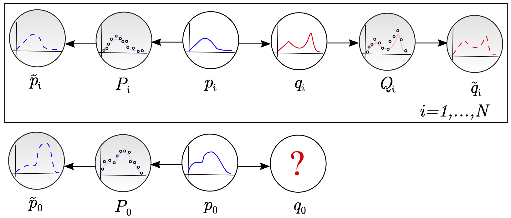
Figure 2: We observe a data-set of input/output functional observation pairs $\{(P_{i},Q_{i})\}_{i=1}^{N}$, where $P_{i}$, $Q_{i}$ are some inexact observations of functions $p_{i}$ and $q_{i}$ such as a set of noisy function evaluations at uniformly distributed points. $P_{i}$, $Q_{i}$ then are used to make function approximations $\tilde{p}_{i},\tilde{q}_{i}$, which in turn are used to predict the response $q_{0}$ for a unseen query input function $p_{0}$.

Our approach will be as follows. First, we convert the infinite dimensional task of estimating the output function $q_{0}$ into a finite dimensional problem by projecting $q_{0}$ into a finite number of basis functions (focusing on the crucial characteristics of $q_{0}$, roughly speaking). Then, to estimate the projections onto the basis functions we embed the input functions into a nonlinear space where linear operations are approximately evaluations of a nonlinear mapping $f$ in a broad function class. Finally, $f$ is estimated by empirically minimizing the risk of a linear operation in the nonlinear embedding of input functions for predicting the basis projections of output functions in a dataset.

Our Contribution

We develop the Triple-Basis Estimator (3BE), a novel nonparametric estimator for FFR that scales to large data-sets. The 3BE is the first estimator of its kind, allowing one to regress functional responses given functional covariates in massive data-sets. Furthermore, we analyze the $L_{2}$ risk of the 3BE under nonparametric assumptions. Lastly, we show an improvement of several orders of magnitude over existing estimators in terms of prediction time as well as a reduction in error in various real-world data-sets.

2 Related Work

A previous nonparametric FFR estimator was proposed in [4]. [4] attempts to perform FFR on a functional RKHS. That is, if we consider $\mathcal{F}$ as a functional Hilbert space, where $f\in\mathcal{F}$ is such that $f:\mathcal{G}_{x}\mapsto\mathcal{G}_{y}$, then $f$ is estimated by $f^{*}=\operatorname*{arg\,min}_{\hat{f}}\sum_{i=1}^{N}\lVert q_{i}-\hat{f}(p_{i})\rVert^{2}_{\mathcal{G}_{y}}+\lambda\lVert f\rVert^{2}_{\mathcal{F}}.$ However, when each function is observed though $n$ noisy function evaluations this estimator will require the inversion of a $Nn\times Nn$ matrix, which will be computationally infeasible for data-sets of even a modest size.

In addition, [8] provides an estimator for doing FFR for the special case where both input and output functions are probability distribution functions. The estimator, henceforth referred to as the linear smoother estimator (LSE), works as follows when given a training data-sets of $\mathcal{D}=\{(P_{i},Q_{i})\}_{i=1}^{N}$ of empirical functional observations and $\tilde{\mathcal{D}}=\{(\tilde{p}_{i},\tilde{q}_{i})\}_{i=1}^{N}$ of function estimates and a function estimate $\tilde{p}_{0}$ of a new query input function:

$$\hat{f}(\tilde{p}_{0}) =\sum_{i=1}^{N}W(\tilde{p}_{i},\tilde{p}_{0})\tilde{q}_{i}\ \mathrm{where}\$$ (1)

$$W(\tilde{p}_{i},\tilde{p}_{0}) =\begin{cases}\frac{K(D(\tilde{p}_{i},\tilde{p}_{0}))}{\sum\limits_{j=1}^{N}K(D(\tilde{p}_{j},\tilde{p}_{0}))}&\mbox{if }\sum_{j}K(D(\tilde{p}_{j},\tilde{p}_{0}))>0\\ 0&\mbox{otherwise }.\end{cases}$$ (2)

Here $K:\mathbb{R}\rightarrow[0,\infty)$ is taken to be a symmetric kernel with bounded support, and $D$ is some metric over functions. However, while such an estimator is useful for smaller FFR problems, it may not be used in larger data-sets. Clearly, the LSE must perform a kernel evaluation with all input distributions in one’s data-set to produce a prediction, leading to a total computational cost of $\Omega(Nn)$ when considering the cost of computing metrics $D(\tilde{p}_{j},\tilde{p}_{0})$ when $|P_{i}|\asymp|Q_{i}|\asymp n$. This implies, for example, that obtaining estimates for each training instance scales as $\Omega(nN^{2})$, which will be prohibitive for big data-sets.

Previous work for nonparametric estimation in large data-sets with functional inputs includes [7]. There an estimator was proposed for scalable learning of a distribution input covariate to real-value output response regression problem. We note however that it is not immediately clear how to achieve a scalable estimator for regression functional responses with functional covariates, nor how to analyze such an estimator’s risk since general functional responses are infinite dimensional.

We note further that work has been done in linear models for FFR (e.g. [11, 9]). However, such models work over a strong assumption on the linearity of the mapping $f$, and will not be able to capture non-linear mappings. Moreover, FFR is a specific case of general functional analysis [11, 1, 12].

3 Model

We expound upon our model of input/output functions and the mapping between them. Later, we introduce the 3BE and its risk for the case when one has a data-set of pairs of input/output functional observations that are a set of noisy function evaluations at uniformly distributed points. However, the following is generalizable for the case where one observes function evaluations at a fixed grid of points or function observations of samples from distributions. In short, we assume smooth input/output functions that are well approximated by a finite number of basis functions. Further, we consider a nonparametric mapping between them, where the projection of the output function onto each basis function may be written as an infinite linear combination of RBF kernel evaluations between the input function and unknown functions (see below).

We take our data-set to be input/output empirical function observation pairs:

$$\mathcal{D} =\{(P_{i},Q_{i})\}_{i=1}^{N}\ \mathrm{where}\$$ (3)

$$P_{i} =\left\{p_{i}(u_{ij})+\epsilon_{ij}\right\}_{j=1}^{n_{i}},\ Q_{i}=\left\{q_{i}(v_{ij})+\xi_{ij}\right\}_{j=1}^{m_{i}},$$ (4)

with sample points $u_{ij}\overset{iid}{\sim}\operatorname*{Unif}([0,1]^{l})$, $v_{ij}\overset{iid}{\sim}\operatorname*{Unif}([0,1]^{k})$, and noise $\epsilon_{ij}\overset{iid}{\sim}\Xi_{\epsilon}$, $\xi_{ij}\overset{iid}{\sim}\Xi_{\xi}$. With error distributions $\Xi_{\xi},\Xi_{\epsilon}$, s.t. $\mathbb{E}\left[\epsilon_{ij}\right]=\mathbb{E}\left[\xi_{ij}\right]=0$, $\operatorname*{Var}\left[\epsilon_{ij}\right],\operatorname*{Var}\left[\xi_{ij}\right]\leq\varsigma<\infty$. Furthermore, $p_{i}\in\mathcal{I}$, $p_{i}:[0,1]^{l}\mapsto\mathbb{R}$, $q_{i}\in\mathcal{O}$, $q_{i}:[0,1]^{k}\mapsto\mathbb{R}$, $q_{j}=f(p_{j})$, and $p_{i}\overset{iid}{\sim}\Phi$ where $\mathcal{I}$ and $\mathcal{O}$ are some class of input/output functions and $\Phi$ is some measure over $\mathcal{I}$. Furthermore, we shall assume that $n_{i}\asymp n$ and $m_{i}\asymp m$. We shall use $\mathcal{D}$ to make estimates of the true input/output functions $\tilde{D}=\{(\tilde{p}_{i},\tilde{q}_{i})\}_{i=1}^{N}$, which will then be used to estimate the output function $q_{0}$ corresponding to an unseen input function $p_{0}$.

3.1 Basis Functions and Projections

Let $\{\varphi_{i}\}_{i\in\mathbb{Z}}$ be an orthonormal basis for $L_{2}([0,1])$. Then, the tensor product of $\{\varphi_{i}\}_{i\in\mathbb{Z}}$ serves as an orthonormal basis for $L_{2}([0,1]^{d})$; that is, the following is an orthnormal basis for $L_{2}([0,1]^{d})$

$$\{\varphi_{\alpha}\}_{\alpha\in\mathbb{Z}^{d}}\quad\mathrm{where}\quad\varphi_{\alpha}(x)=\prod_{i=1}^{d}\varphi_{\alpha_{i}}(x_{i}),\ x\in[0,1]^{d}.$$

So we have that $\forall\alpha,\rho\in\mathbb{Z}^{d},\ \langle\varphi_{\alpha},\varphi_{\rho}\rangle=I_{\{\alpha=\rho\}}$. Let $h\in L_{2}([0,1]^{d})$, then

$$h(x) =\sum_{\alpha\in\mathbb{Z}^{d}}a_{\alpha}(h)\varphi_{\alpha}(x)\quad\mathrm{where}$$ (5)

$$\quad a_{\alpha}(h) =\langle\varphi_{\alpha},h\rangle=\int_{[0,1]^{d}}\varphi_{\alpha}(z)h(z)\mathrm{d}z\ \in\mathbb{R}.$$ (6)

As previously mentioned, a data-set of estimated input/output function pairs, $\tilde{\mathcal{D}}=\{(\tilde{p}_{i},\tilde{q}_{i})\}_{i=1}^{N}$, will be constructed from the data-set of input/output function evaluation sets $\mathcal{D}=\{(P_{i},Q_{i})\}_{i=1}^{N}$. Suppose function $h$ has a corresponding set of evaluations $H=\{y_{j}=h(u_{j})+\epsilon_{j}\}_{j=1}^{r}$ where $u_{j}\overset{iid}{\sim}\operatorname*{Unif}([0,1]^{d})$ and $\mathbb{E}\left[\epsilon_{j}\right]=0$, $\mathbb{E}\left[\epsilon_{j}^{2}\right]<\infty$. Then, $\tilde{h}$, the estimate of $h$, will be as follows:

$$\tilde{h}(x) =\sum_{\alpha\in M}a_{\alpha}(H)\varphi_{\alpha}(x)\quad\mathrm{where}$$ (7)

$$a_{\alpha}(H) =\frac{1}{r}\sum_{j=1}^{r}y_{j}\varphi_{\alpha}(u_{j}),$$ (8)

and $M$ is a finite set of indices for basis functions.

3.1.1 Cross-validation

In practice, one would choose indices $M$ in (8) through cross-validation. The number of projection coeffients one chooses will depend on the smoothness of the function $h$ aswell as the number of points in $H$. Typically, a larger $|i|$ will correspond to a higher frequency 1-dimensional basis function $\varphi_{i}$; thus, a natural way of selecting $M$ is to consider sets

$$M_{t}=\{\alpha\in\mathbb{Z}^{d}:\lVert\alpha\rVert_{2}\leq t\}$$ (9)

with $t\in(0,\infty)$. One would then choose the value of $t$ (setting $M=M_{t}$) that minimizes a loss, such as the mean squared error between $\tilde{h}(u_{i})$ and $y_{i}$. We shall see below that considering $M_{t}$ in this manner corresponds to a smoothness assumption on the class of input/output functions.

3.2 Function to Function Mapping

Let $p\sim\Phi$, $q=f(p)$, as in (32), we have that

$$q(x)=[f(p)](x) =\sum_{\alpha\in\mathbb{Z}^{k}}a_{\alpha}(f(p))\varphi_{\alpha}(x)$$ (10)

$$=\sum_{\alpha\in\mathbb{Z}^{k}}f_{\alpha}(p)\varphi_{\alpha}(x)$$ (11)

where $f_{\alpha}(p)=a_{\alpha}(f(p))$. Hence we may think of $f:\mathcal{I}\mapsto\mathcal{O}$ as consisting of countably many functions $\{f_{\alpha}\ |\ f_{\alpha}:\mathcal{I}\mapsto\mathbb{R},\ \alpha\in\mathbb{Z}^{k}\}$, where each $f_{\alpha}$ is responsible for the mapping of $p$ to the projection of $q$ on to $\varphi_{\alpha}$. We take $f_{\alpha}$ functions to be a nonparametric linear smoother on a possibly infinite set of functions weighted by a kernel:

$$f_{\alpha}(p)=\sum_{i=1}^{\infty}\theta_{\alpha i}K_{\sigma}(g_{\alpha i},p)\ \mathrm{where}$$ (12)

$$\theta_{\alpha i}\in\mathbb{R},\ g_{\alpha i}\in\mathcal{I}$$ (13)

We shall consider the following class of functions:

$$\mathcal{F}_{\sigma} =\{f\ :\ \forall\alpha\in\mathbb{Z}^{k}\ \lVert\theta_{\alpha}\rVert_{1}\leq B_{\alpha},f_{\alpha}\text{ as in }\eqref{eq:q_form}\}.$$ (14)

4 Triple-Basis Estimator

If the tail-frequency behavior of output functions are controlled, then we may effectively estimate output functions using a finite number of projection coefficients; thus, we only need to estimate a finite number of the $f_{\alpha}$ functions. The 3BE consists of two orthonormal bases for estimating input and output functions respectively and a random basis to estimate the mapping between them. To efficiently estimate the $f_{\alpha}$ functions, we shall use random basis functions from Random Kitchen Sinks (RKS) [10]. We shall show that to approximate $f_{\alpha}$, we need only estimate a linear mapping in the random RKS features. [10] shows that if one has a shift-invariant kernel $K$ (in particular we consider the RBF kernel $K(x)=\exp(-x^{2}/2)$), then for fixed $\omega_{i}\stackrel{{\scriptstyle iid}}{{\sim}}\mathcal{N}(0,\sigma^{-2}I_{d})$, $b_{i}\stackrel{{\scriptstyle iid}}{{\sim}}\operatorname*{Unif}([0,2\pi])$, we have that for each $x,y\in\mathbb{R}^{d}$:

$$K(\left\lVert x-y\right\rVert_{2}/\sigma)\approx z(x)^{T}z(y),\ \mathrm{where}$$ (15)

$$z(x)\equiv\sqrt{\tfrac{2}{D}}\left[\cos(\omega_{1}^{T}x+b_{1})\cdots\cos(\omega_{D}^{T}x+b_{D})\right]^{T},$$ (16)

and $D$ is the number of random basis functions (see [10] for approximation quality) . Let $U$ and $V$ be a set of indices for basis functions to project input and output functions respectively:

$$U=\{\alpha_{1},\ldots,\alpha_{s}\},V=\{\beta_{1},\ldots,\beta_{r}\}.$$ (17)

In practice one would choose $U$ and $V$ through cross-validation (see $\S$3.1.1). First note that:

$$\langle\tilde{p}_{i},\tilde{p}_{j}\rangle =\left\langle\sum_{\alpha\in U}a_{\alpha}(P_{i})\varphi_{\alpha},\sum_{\alpha\in U}a_{\alpha}(P_{j})\varphi_{\alpha}\right\rangle$$ (18)

$$=\sum_{\alpha\in U}\sum_{\beta\in U}a_{\alpha}(P_{i})a_{\beta}(P_{j})\left\langle\varphi_{\alpha},\varphi_{\beta}\right\rangle$$ (19)

$$= \sum_{\alpha\in U}a_{\alpha}(P_{i})a_{\alpha}(P_{j})=\left\langle\vec{a}_{U}(P_{i}),\vec{a}_{U}(P_{j})\right\rangle,$$ (20)

where $\vec{a}_{U}(P_{i})=(a_{\alpha_{1}}(P_{i}),\ldots,a_{\alpha_{s}}(P_{i}))^{T}$. Thus, $\left\lVert\tilde{p}_{i}-\tilde{p}_{j}\right\rVert_{2}=\left\lVert\vec{a}_{U}(P_{i})-\vec{a}_{U}(P_{j})\right\rVert_{2},$ where the norm on the LHS is the $L_{2}$ norm and the $\ell_{2}$ on the RHS.

Consider a fixed $\sigma$, and let $\omega_{i}\stackrel{{\scriptstyle iid}}{{\sim}}\mathcal{N}(0,\sigma^{-2}I_{s})$, $b_{i}\stackrel{{\scriptstyle iid}}{{\sim}}\operatorname*{Unif}[0,2\pi]$, be fixed. Then

$$f_{\alpha}(p_{0}) =\sum_{i=1}^{\infty}\theta_{\alpha i}K_{\sigma}(\lVert g_{\alpha i}-p_{0}\rVert_{2})$$ (21)

$$\approx\sum_{i=1}^{\infty}\theta_{\alpha i}K_{\sigma}(\lVert\vec{a}_{U}(g_{\alpha i})-\vec{a}_{U}(P_{0})\rVert_{2})$$ (22)

$$\approx\sum_{i=1}^{\infty}\theta_{\alpha i}z(\vec{a}_{U}(g_{\alpha i}))^{T}z(\vec{a}_{U}(P_{0}))$$ (23)

$$=\hskip 2.84526pt\psi_{\alpha}^{T}z(\vec{a}_{U}(P_{0}))$$ (24)

where $\psi_{\alpha}=\sum_{i=1}^{\infty}\theta_{\alpha i}z(\vec{a}_{U}(g_{\alpha i}))\in\mathbb{R}^{s}$. Hence, by (24) $f_{\alpha}$ is approximately linear in $z(\vec{a}_{U}(\cdot))$; so, we consider linear estimators in the non-linear space induced by $z(\vec{a}_{U}(\cdot))$. In particular, we take the OLS estimator using the data-set $\{(z(\vec{a}_{U}(P_{i})),a_{\alpha}(Q_{i}))\}_{i=1}^{N}$, and for each $f_{\alpha}$ we estimate :

$$\hat{f}_{\alpha}(P_{0}) \equiv\hat{\psi}^{T}_{\alpha}z(\vec{a}_{U}(P_{0}))\quad\mathrm{where}$$ (25)

$$\hat{\psi}_{\alpha} \equiv\operatorname*{arg\,min}_{\beta}\lVert\vec{A}_{\alpha}-{\bf{Z}}\beta\rVert_{2}^{2}=({\bf{Z}}^{T}{\bf{Z}})^{-1}{\bf{Z}}^{T}\vec{A}_{\alpha}$$ (26)

for $\vec{A}_{\alpha}=(a_{\alpha}(Q_{1}),\ldots,a_{\alpha}(Q_{N}))^{T}$, and ${\bf{Z}}$ the $N\times D$ matrix ${\bf{Z}}=[z(\vec{a}_{U}(P_{1}))\cdots z(\vec{a}_{U}(P_{N}))]^{T}$. Suppose that the indices of basis functions we project output function onto is $V$ (as in (17)), then the set of functions we estimate is $\{\hat{f}_{\alpha}\ :\ \alpha\in V\}$. Let $\hat{f}_{1:r}(P_{0})=(\hat{f}_{\alpha_{1}}(P_{0}),\ldots,\hat{f}_{\alpha_{r}}(P_{0}))^{T}$, ${\bf{A}}_{1:r}=[\vec{A}_{\alpha_{1}},\ldots,\vec{A}_{\alpha_{r}}]\in\mathbb{R}^{N\times r}$:

$$\hat{f}_{1:r}(P_{0}) =\hat{\Psi}^{T}z(\vec{a}_{U}(P_{0}))\quad\mathrm{where}$$ (27)

$$\hat{\Psi} =({\bf{Z}}^{T}{\bf{Z}})^{-1}{\bf{Z}}^{T}{\bf{A}}_{1:r}.$$ (28)

4.1 Evaluation Computational Complexity

We see that after computing $\hat{\Psi}$, evaluating the estimated projection coefficients for a new function $p_{0}$ amounts to performing a matrix multiplication of a $r\times D$ matrix with a $D\times 1$ vector. Including the time required for computing $z(\vec{a}_{U}(P_{0}))$, the computation required for the evaluation, (28), is: 1) the time for evaluating the projection coefficients $\vec{a}_{U}(P_{0})$, $O(sn)$; 2) the time to compute the RKS features $z(\cdot)$, $O(Ds)$; 3) the time to compute the matrix multiplication, $\hat{\Psi}^{T}z(\vec{a}_{U}(P_{0}))$, $O(rD)$. Hence, the total time is $O(rD+Ds+sn)$.

We’ll see that we may choose $D=O(n\log(n))$, $s=O(n)$, and $r=O(m)$. If we assume further that $m\asymp n$, the total runtime for evaluating $\hat{f}(\tilde{p}_{0})$ is $O(n^{2}\log(n))$. Since we are considering data-sets where the number of instances $N$ far outnumbers the number of points per sample set $n$, $O(n^{2}\log(n))$ is a substantial improvement over $\Omega(Nn)$ for the LSE; indeed, the LSE requires a metric evaluation with every training-set input function (2) where the 3BE does not. Furthermore, the space complexity is much improved for the 3BE since we only need to store the $O(n^{2}\log(n))$ matrix $\Psi$ and the $O(n^{2}\log(n))$ total space for the RKS basis functions $\{(\omega_{i},b_{i})\}$. Contrast this with the space required for the LSE, $\Omega(Nn)$, which is much larger for our case of $n\ll N$. Lastly, note that to evaluate $\hat{q}_{0}(x)=[\hat{f}(P_{0})](x)$ once one has computed $\hat{f}_{1:r}(P_{0})$, one only needs to compute $\hat{q}_{0}(x)=\langle\hat{f}_{1:r}(P_{0}),\vec{\varphi}_{1:r}(x)\rangle$ where $\vec{\varphi}_{1:r}(x)=(\varphi_{\alpha_{1}}(x),\ldots,\varphi_{\alpha_{r}}(x))$.

Triple-Basis Estimator

We note that a straightforward extension to the 3BE is to use a ridge regression estimate on features $z(\vec{a}_{t}(\cdot))$ rather than a OLS estimate. That is, for $\lambda\geq 0$ let

$$\hat{\psi}_{\alpha\lambda} \equiv\operatorname*{arg\,min}_{\beta}\lVert\vec{A}_{\alpha}-{\bf{Z}}\beta\rVert_{2}^{2}+\lambda\lVert\beta\rVert_{2}^{2}$$ (29)

$$=({\bf{Z}}^{T}{\bf{Z}}+\lambda I)^{-1}{\bf{Z}}^{T}\vec{A}_{\alpha}.$$ (30)

The Ridge-3BE is still evaluated via a matrix multiplication, and our complexity analysis holds.

4.2 Algorithm

We summarize the basic steps for training the 3BE in practice given a data-set of empirical functional observations $\mathcal{D}=\{(P_{i},Q_{i})\}_{i=1}^{N}$, parameters $\sigma$ and $D$ (which may be cross-validated), and an orthonormal basis $\{\varphi_{i}\}_{i\in\mathbb{Z}}$ for $L_{2}([0,1])$.

1. Determine the sets of basis functions $U$ and $V$ (17) for approximating $p$, and $q$ respectively. For each $j$ in a subset $J\subseteq\{1,\ldots,N\}$ one can select a set $M_{t_{j}}$ (9) to estimate $p_{j}$ by cross-validating a loss as described in $\S$ 3.1.1. One may then set $U=M_{\bar{t}}$ where $\bar{t}=\frac{1}{|J|}\sum_{j\in J}t_{j}$. Similarly, one may set $V=M_{\bar{c}}$ by cross-validating $M_{c_{j}}$’s for $q_{j}$’s.

2. Let $s=|U|$, draw $\omega_{i}\stackrel{{\scriptstyle iid}}{{\sim}}\mathcal{N}(0,\sigma^{-2}I_{s})$, $b_{i}\stackrel{{\scriptstyle iid}}{{\sim}}\operatorname*{Unif}[0,2\pi]$ for $i\in\{1,\ldots,D\}$; keep the set $\{(\omega_{i},b_{i})\}_{i=1}^{D}$ fixed henceforth.

3. Let $\{\alpha_{1},\ldots,\alpha_{r}\}=V$. Generate the data-set of random kitchen sink features, output projection coefficient vector pairs $\{(z(\vec{a}_{U}(P_{i})),\vec{a}_{V}(Q_{i}))\}_{i=1}^{N}$. Let $\hat{\Psi}=({\bf{Z}}^{T}{\bf{Z}})^{-1}{\bf{Z}}^{T}{\bf{A}}_{1:r}\in\mathbb{R}^{D\times r}$ where ${\bf{Z}}=[z(\vec{a}_{U}(P_{1}))\cdots z(\vec{a}_{U}(P_{N}))]^{T}\in\mathbb{R}^{N\times D}$, ${\bf{A}}_{1:r}=[\vec{A}_{\alpha_{1}},\ldots,\vec{A}_{\alpha_{r}}]\in\mathbb{R}^{N\times r}$. Note that ${\bf{Z}}^{T}{\bf{A}}_{1:r}$ and ${\bf{Z}}^{T}{\bf{Z}}$ can be computed efficiently using parallelism.

4. For all future query input functional observations $P_{0}$, estimate the projection coefficients of the corresponding output function as $\hat{f}_{1:r}(P_{0})=\hat{\Psi}^{T}z(\vec{a}_{U}(P_{0}))$.

5 Theory

We analyze the $L_{2}$ risk for the 3BE estimator below. We assume that input/output functions belong to a Sobolev Ellipsoid function class and that the mapping between input and output functions is in $\mathcal{F}_{\sigma}$ (14).

5.1 Assumptions

5.1.1 Sobolev Ellipsoid Function Classes

We shall make a Sobolev ellipsoid assumption for classes $\mathcal{I}$ and $\mathcal{O}$. Let $a(h)\equiv\{a_{\alpha}(h)\}_{\alpha\in\mathbb{Z}^{d}}$. Suppose that the projection coefficients $a(p)=\{a_{\alpha}(p)\}_{\alpha\in\mathbb{Z}^{l}}$ and $a(q)=\{a_{\alpha}(q)\}_{\alpha\in\mathbb{Z}^{k}}$ are as follows for $p\in\mathcal{I}$, $q\in\mathcal{O}$:

$$\mathcal{I} =\{p:a(p)\in\Theta_{l}(\nu_{\scriptscriptstyle\mathcal{I}},\gamma_{\scriptscriptstyle\mathcal{I}},A_{\scriptscriptstyle\mathcal{I}}),\lVert p\rVert_{\infty}\leq A_{\scriptscriptstyle\mathcal{I}}\}$$ (31)

$$\mathcal{O} =\{q:a(q)\in\Theta_{k}(\nu_{\scriptscriptstyle\mathcal{O}},\gamma_{\scriptscriptstyle\mathcal{O}},A_{\scriptscriptstyle\mathcal{O}}),\lVert q\rVert_{\infty}\leq A_{\scriptscriptstyle\mathcal{O}}\}$$ (32)

where $\nu_{\scriptscriptstyle\mathcal{I}},\gamma_{\scriptscriptstyle\mathcal{I}}\in\mathbb{R}_{++}^{l}$, $\nu_{\scriptscriptstyle\mathcal{O}},\gamma_{\scriptscriptstyle\mathcal{O}}\in\mathbb{R}_{++}^{k}$, $A_{\scriptscriptstyle\mathcal{I}},A_{\scriptscriptstyle\mathcal{O}}\in\mathbb{R}_{++}$, $\mathbb{R}_{++}=(0,\infty)$, and

$$\Theta_{d}(\nu,\gamma,A) =\Big{\{}\{a_{\alpha}\}_{\alpha\in\mathbb{Z}^{d}}:\sum_{\alpha\in\mathbb{Z}^{d}}a_{\alpha}^{2}\kappa_{\alpha}^{2}(\nu,\gamma)<A\Big{\}}$$ (33)

$$\kappa_{\alpha}^{2}(\nu,\gamma) =\sum_{i=1}^{d}(\nu_{i}|\alpha_{i}|)^{2\gamma_{i}}\ \mathrm{for}\ \nu_{i},\gamma_{i},A>0.$$ (34)

See [3, 5] for other work using similar Sobolev elipsoid assumptions. The assumption in (32) will control the tail-behavior of projection coefficients and allow one to effectively estimate $p\in\mathcal{I}$ and $q\in\mathcal{O}$ using a finite number of projection coefficients on the empirical functional observation.

Suppose as before that function $h$ is such that $a(h)\in\Theta_{d}(\nu,\gamma,A)$ has a corresponding set of evaluations $H=\{y_{j}=h(u_{j})+\epsilon_{j}\}_{j=1}^{r}$ where $u_{j}\overset{iid}{\sim}\operatorname*{Unif}([0,1]^{d})$ and $\mathbb{E}\left[\epsilon_{j}\right]=0$, $\mathbb{E}\left[\epsilon_{j}^{2}\right]<\infty$. Then, $\tilde{h}$, the estimate of $h$, is:

$$\tilde{h}(x) =\sum_{\alpha\ :\ \kappa_{\alpha}(\nu,\gamma)\leq t}a_{\alpha}(H)\varphi_{\alpha}(x)\quad\mathrm{where}$$ (35)

$$a_{\alpha}(H) =\frac{1}{r}\sum_{j=1}^{r}y_{j}\varphi_{\alpha}(u_{j}).$$ (36)

Choosing $t$ optimally can be shown to lead to $\mathbb{E}[\lVert\tilde{h}-h\rVert_{2}^{2}]=O(r^{-\frac{2}{2+\gamma^{-1}}})$, where $\gamma^{-1}=\sum_{j=1}^{d}\gamma_{j}^{-1}$, $r\rightarrow\infty$. Thus, we can represent $h$ using a finite number of projection coefficients $\vec{a}_{t}(H)=(a_{\alpha}(H):\kappa_{\alpha}(\nu,\gamma)\leq t)^{T}$; this allows one to approximate the FFR problem as a regression problem over finite vectors $\vec{a}_{t}(p)$ and $\vec{a}_{t^{\prime}}(q)$. Note that our choice of sets $M_{t}$ (9) in $\S$3.1.1 corresponds to the estimator in (36) with $\nu,\gamma=\vec{1}$. Varying $t$ in this case will still be adaptive to the smoothness of $h$, and the number of points in $H$.

5.1.2 Function to Funcion Mapping

Recall that we take output functions to be:

$$q(x)=[f(p)](x) =\sum_{\alpha\in\mathbb{Z}^{k}}f_{\alpha}(p)\varphi_{\alpha}(x)$$

where $f_{\alpha}(p)=a_{\alpha}(f(p))$. An our assumption of the class of mappings is:

$$\mathcal{F}_{\sigma} =\{f\ :\ \forall\alpha\in\mathbb{Z}^{k}\ \lVert\theta_{\alpha}\rVert_{1}\leq B_{\alpha},f_{\alpha}\text{ as in }\eqref{eq:q_form}\}$$

Suppose further that:

$$\sum_{\alpha\in\mathbb{Z}^{k}}B_{\alpha}^{2}\kappa_{\alpha}^{2}(\nu_{\scriptscriptstyle\mathcal{O}},\gamma_{\scriptscriptstyle\mathcal{O}})\leq A_{\scriptscriptstyle\mathcal{O}}.$$ (37)

Hence, if $f\in\mathcal{F}_{\sigma}$ then $q=f(p)\implies q\in\mathcal{O}$ since $|f_{\alpha}(p)|\leq\lVert\theta_{\alpha}\rVert_{1}\leq B_{\alpha}$ and (37) holds.

5.2 Risk Upperbound

Below we state our main theorem, upperbounding the risk of the 3BE.

Theorem 5.1.

Let a small constant $\delta>0$ be fixed. Suppose that $\hat{q}_{0}(x)=\sum_{\alpha\in M^{\scriptscriptstyle\mathcal{O}}_{u}}\hat{f}_{\alpha}(P_{0})\varphi_{\alpha}(x)$, $\hat{f}_{\alpha}(P_{0})$ given by (26). Furthermore, suppose that (32) holds and $f\in\mathcal{F}_{\sigma}$ as in (37). Moreover, assume that (4) holds and $n_{i},m_{i}\asymp n$. Also, assume that the number of RKS features $D$ (16) is taken to be $D\asymp n\log(n)$. Then,

$$\mathbb{E}\left[\lVert q_{0}-\hat{q}_{0}\rVert^{2}_{2}\right]$$ (38)

$$\leq O\left(\left(n^{-1/(2+\gamma_{\scriptscriptstyle\mathcal{I}}^{-1})}+\frac{n\log(n)\log(N)}{N}\right)^{2/(2+\gamma_{\scriptscriptstyle\mathcal{O}}^{-1})}\right)$$ (39)

$$\text{with probability at least }1-\delta.$$

See appendix for proof. The rate (39) yields consistency for our estimator if $n\log(n)=o(N/\log(N))$; that is, so long as one is in the large data-set domain where the number of instances is larger than the number of points in function observations. Note that the first summand in (39) is similar to typical functional estimation rates, and it stems from our approximation with bases; the second summand is akin to a linear regression rate, and it stems from our OLS estimation (26).

6 Experiments

Below we show the improvement of the 3BE over previous FFR approaches in several real-world data-sets. Empirically, the 3BE proves to be the most general, quickest, and effective estimator. Unlike previous time-series FFR approaches, the 3BE easily lends itself to working over distributions. Moreover, unlike previous nonparametric FFR estimators the 3BE does not need to compute pairwise kernel evaluations, making it much more scalable. All differences in MSE were statistically significant ($p<0.05$) using paired t-tests.

6.1 Rectifying 2LPT Simulations

Numerical simulations have become an essential tool to study cosmological structure formation. Astrophysics use N-body simulations [15] to study the gravitational evolution of collisionless particles like dark matter particles. Unfortunately, N-body simulations require forces among particles to be recomputed over multiple time intervals, leading to a large magnitude of time steps to complete a single simulation. In order to mitigate the large computational costs of running N-body simulations, often simulations based on Second Order Lagrange Perturbation Theory (2LPT) [13] are used.

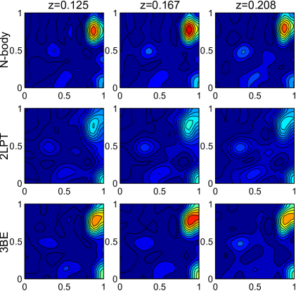
Figure 3: Slices of particle pdfs.

Although 2LPT simulations are several orders of magnitude faster, they prove to be inaccurate, especially at smaller scales. In this experiment we bridge the gap between the speed of 2LPT simulations and the accuracy of N-body simulations using FFR and the 3BE. Namely, we regress the mapping between a distribution of particles in an area coming from a 2LPT simulation and the distribution of the particles in the same area under an equivalent N-body simulation.

Method	MSE	MPT
3BE	4.958	0.009
LSE	6.816	4.977
2LPT	6.424	NA
AD	9.289	NA

Table 1: MSE and MPT(s) results.

We regress the distribution of 3d (spatial) N-body simulation particles in $16\ \mathrm{Mpc}^{3}$ cubes when given the distribution of particles of the 2LPT simulation in the same cube (note that each distribution is estimated through the set of particles in each cube). A training-set of over 900K pairs of 2LPT cube sample-set/N-body cube sample-set instance was used, along with a test-set of 5K pairs. The number of projection coefficients used to represent input and output distributions was 365/401 respectively, chosen by cross-validating the density estimates. We chose the number of RKS features to be 15K based on rules-of-thumb. We cross-validated the $\sigma$ and $\lambda$ parameters of the ridge variant 3BE (30) and the smoothing parameter of the LSE and reported back the MSE and mean prediction time (MPT, in seconds) of our FFR estimates to the distributions truly coming directly through N-body simulation (Table 1); we also report the MSE of predicting the average output distribution (AD).

We see that the 3BE is about $500\times$ faster than the LSE in terms of prediction time and achieved an improvement in $R^{2}$ of over $50\%$ over using the distribution coming directly from the 2LPT simulation (2LPT). Note also that the LSE does not achieve an improvement in MSE over 2LPT.

6.2 Time-series Data

We compared the performance of the 3BE in time-series prediction problems to using the LSE and widely used time-series prediction methods like Dynamics Mining with Missing values (DynaMMo) [6] and Kernel Embedded HMMs (SHMM) [14]. DynaMMo is a latent-variable probabilistic model trained with EM aimed at predicting data that is missing in chunks and not just in a single time-step (as we also attempt with our functional responses).

6.2.1 Forward Prediction with Music Data

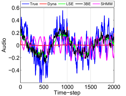
Figure 4: Example audio predictions; segments separated with vertical lines.

Music data presents a particularly interesting application of forward prediction for time-series. That is, given a short segment of audio data from a piece of music, can we predict the audio data in the short segment that follows? Uses for forward prediction with music include compression and music similarity.

In this experiment, we use a 30 second clip, sampled at 44.1 kHz from the song “I Turn To You” by the artist Melanie C. We extract a mono signal of the sound clip and use the first $85\%$ for training and hold-out, and the final $15\%$ for testing. To perform forward prediction in the test set, we take a $500$ time-step segment of the (true) music time-series as input and use it to predict the following $500$ time-steps. We repeat this sequentially over consecutive disjoint segments in the test set until we have made predictions for the entire test set. In total our data-set consisted of about $2,200$ training instances. For audio prediction with the 3BE we use the ridge variant (30). We use 150 trigonometric basis functions for both input and output functions, and 5000 RKS basis functions (both quantities chosen via rules of thumb). We then cross-validate the bandwidth and $\lambda$ penalty parameters.

Method	MSE
3BE	0.0327
LSE	0.0351
Dyna	0.0492
SHMM	0.1082

Table 2: Audio MSE.

We cross-validated the number of dimensions for hidden-states for DynaMMo, and the bandwidth parameter for the LSE. The mean squared error (MSE) on the test-set is reported in Table 2 for each method. The 3BE achieves the lowest estimation error. Furthermore, looking at Figure 4 it is apparent that the 3BE outperforms the other methods in terms of capturing the structure of the audio data. The quality of the audio predicted with the 3BE is also superior to the other methods (hear predicted sound clips in supplemental materials). Furthermore, DynaMMo takes over 4 hours to learn a model given a fixed hidden state dimensionality with no missing data (and even longer if also predicting missing data), where as the 3BE takes only about 2 minutes to cross-validate and perform predictions (a speed-up of over $7000\times$). Similarly the 3BE was over $5000\times$ faster than SHMM for predictions. Additionally, even though the data-set is of a smaller scale, the 3BE still enjoys a $3\times$ speedup over LSE for prediction time.

6.2.2 Co-occurring Predictions with Joint Motion Capture Data

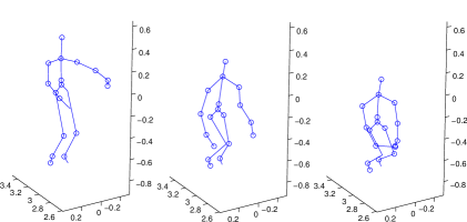
Figure 5: Example “duck” frames.

Next, we explore predicting co-occurring time-series with motion capture (MoCap) data. We use the MSRC-12 Data-set [2]. The 3d positions are provided for 20 total joints. We look to predict the time-series of the position of an unobserved joint over a $T$ time-step segment given time-series data (one function for each joint’s x, y, or z position) for $R$ observed joints for the segment.

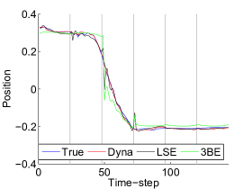
Figure 6: Occluded joint predictions.

We performed co-occurring time-series prediction with MoCap data of a subject performing the gesture “duck” (Figure 5). We randomly chose 10 joints to designate as occluded, and used the other 10 as our non-occluded joints. We then solved 30 separate FFR problems, where each of the problems had one of the missing joints’ time-series as the output response function (e.g. missing joint 1’s y position or missing joint 4’s x position). In each of the problems, the 30 functions corresponding to the time-series for non-occluded joint spatial positions were used as inputs (by concatenating the projection coefficients of each input function) . We considered segments of 24 time-steps for time-series functions. In total we used a training set of about 1100 instances. The number of projection coefficients for functions was taken to be 10 while the number of RKS features was 250. The same parameters for all estimators were cross validated as before.

Method	MSE
3BE	7.78E-4
LSE	1.3E-3
Dyna	2.40E-4

Table 3: MoCap MSE.

DynaMMo performs the best (Table 3), which is perhaps not surprising given that MoCap occlusion prediction was a point of emphasis for DynaMMo. However, the differences in prediction qualities among the different methods is not as pronounced in this data-set (Figure 6). We again see a speed up of over 1000x using 3BE over DynaMMo, also there was a speed up of over $30\times$ in prediction time over LSE.

7 Conclusion

In conclusion, this paper presents a new estimator, the Triple Basis Estimator (3BE), for performing function to function regression in a scalable manner. Since functional data is complex, it is important to have an estimator that is capable of using massive data-sets in order to achieve a low estimation risk. To the best of our knowledge, the 3BE is the first nonparametric FFR estimator that is capable to scaling to big data-sets. The 3BE achieves this through the use of a basis representation of input and output functions and random kitchen sink basis functions. We analyzed the risk of the 3BE given non-parametric assumptions. Furthermore, we showed an improvement of several orders of magnitude for prediction speed and a reduction in error over previous estimators in various real-world data-sets.

Appendix

Multidimensional Projection Series Functional Estimation

Let $y_{ij}=p_{i}(u_{ij})+\epsilon_{ij}$. Given $P_{i}$ as in (4) our estimator for $p_{i}\in\mathcal{I}$ (32) will be:

$$\tilde{p}_{i}(x)= \sum_{\alpha\ :\ \kappa_{\alpha}(\nu,\gamma)\leq t}a_{\alpha}(P_{i})\varphi_{\alpha}(x)\quad\mathrm{where}$$ (40)

$$a_{\alpha}(P_{i})= \frac{1}{n_{i}}\sum_{j=1}^{n_{i}}y_{ij}\varphi_{\alpha}(u_{ij}).$$ (41)

For readability let $(\nu,\gamma,A)=(\nu_{\scriptscriptstyle\mathcal{I}},\gamma_{\scriptscriptstyle\mathcal{I}},A_{\scriptscriptstyle\mathcal{I}})$. First, note that:

$$\mathbb{E}\left[\lVert p_{i}-\tilde{p}_{i}\rVert_{2}^{2}\right]$$ (42)

$$= \mathbb{E}\left[\left\lVert\sum_{\alpha\in\mathbb{Z}}a_{\alpha}(p_{i})\varphi_{\alpha}-\sum_{\alpha\in M^{\scriptscriptstyle\mathcal{I}}_{t}}a_{\alpha}(P_{i})\varphi_{\alpha}\right\rVert_{2}^{2}\right]$$

$$= \mathbb{E}\Bigg{[}\int_{\Lambda^{l}}\Bigg{(}\sum_{\alpha\in M^{\scriptscriptstyle\mathcal{I}}_{t}}(a_{\alpha}(p_{i})-a_{\alpha}(P_{i}))\varphi_{\alpha}(x)$$

$$+\sum_{\alpha\in(M^{\scriptscriptstyle\mathcal{I}}_{t})^{c}}a_{\alpha}(p_{i})\varphi_{\alpha}(x)\Bigg{)}^{2}\mathrm{d}x\Bigg{]}$$

$$= \mathbb{E}\Bigg{[}\int_{\Lambda^{l}}\sum_{\alpha\in M^{\scriptscriptstyle\mathcal{I}}_{t}}\sum_{\rho\in M^{\scriptscriptstyle\mathcal{I}}_{t}}(a_{\alpha}(p_{i})-a_{\alpha}(P_{i}))$$

$$\qquad\quad(a_{\rho}(p_{i})-a_{\rho}(P_{i}))\varphi_{\alpha}(x)\varphi_{\rho}(x)\mathrm{d}x\Bigg{]}$$

$$+2\mathbb{E}\Bigg{[}\int_{\Lambda^{l}}\sum_{\alpha\in M^{\scriptscriptstyle\mathcal{I}}_{t}}\sum_{\rho\in(M^{\scriptscriptstyle\mathcal{I}}_{t})^{c}}(a_{\alpha}(p_{i})-a_{\alpha}(P_{i}))$$

$$\qquad\qquad a_{\rho}(p_{i})\varphi_{\alpha}(x)\varphi_{\rho}(x)\mathrm{d}x\Bigg{]}$$

$$+\mathbb{E}\Bigg{[}\int_{\Lambda^{l}}\sum_{\alpha\in(M^{\scriptscriptstyle\mathcal{I}}_{t})^{c}}\sum_{\rho\in(M^{\scriptscriptstyle\mathcal{I}}_{t})^{c}}$$

$$\qquad\qquad a_{\alpha}(p_{i})a_{\rho}(p_{i})\varphi_{\alpha}(x)\varphi_{\rho}(x)\mathrm{d}x\Bigg{]}$$

$$= \mathbb{E}\left[\sum_{\alpha\in M^{\scriptscriptstyle\mathcal{I}}_{t}}(a_{\alpha}(p_{i})-a_{\alpha}(P_{i}))^{2}\right]+\mathbb{E}\left[\sum_{\alpha\in(M^{\scriptscriptstyle\mathcal{I}}_{t})^{c}}a_{\alpha}^{2}(p_{i})\right],$$ (43)

where the last line follows from the orthonormality of $\{\varphi\}_{\alpha\in\mathbb{Z}}$. Furthermore, note that $\forall p_{i}\in\mathcal{I}$:

$$\sum_{\alpha\in(M^{\scriptscriptstyle\mathcal{I}}_{t})^{c}}a_{\alpha}^{2}(p_{i})= \frac{1}{t^{2}}\sum_{\alpha\in(M^{\scriptscriptstyle\mathcal{I}}_{t})^{c}}t^{2}a_{\alpha}^{2}(p_{i})$$ (44)

$$\leq \frac{1}{t^{2}}\sum_{\alpha\in\mathbb{Z}}\kappa^{2}_{\alpha}(\nu,\gamma)a_{\alpha}^{2}(p_{i})\leq\frac{A}{t^{2}}.$$ (45)

Also,

$$\mathbb{E}\left[(a_{\alpha}(p_{i})-a_{\alpha}(P_{i}))^{2}\right]= \left(\mathbb{E}\left[a_{\alpha}(P_{i})\right]-a_{\alpha}(p_{i})\right)^{2}$$

$$+\operatorname*{Var}\left[a_{\alpha}(P_{i})\right].$$

We may see that $a_{\alpha}(P_{i})$ is unbiased. Let $u\sim U([0,1]^{l})$, then:

$$a_{\alpha}(p_{i})$$

$$=\int_{\Lambda^{l}}\varphi_{\alpha}(z)p_{i}(z)(1)\mathrm{d}z=\mathbb{E}\left[\varphi_{\alpha}(u)p_{i}(u)\right]$$

$$=\mathbb{E}\left[\frac{1}{n_{i}}\sum_{j=1}^{n_{i}}p(u_{ij})\varphi_{\alpha}(u_{ij})\right]$$

$$=\mathbb{E}\left[\frac{1}{n}\sum_{j=1}^{n}p(u_{ij})\varphi_{\alpha}(u_{ij})\right]+\mathbb{E}\left[\frac{1}{n}\sum_{j=1}^{n}\epsilon_{ij}\varphi_{\alpha}(u_{ij})\right]$$

$$=\mathbb{E}\left[\frac{1}{n_{i}}\sum_{j=1}^{n_{i}}y_{ij}\varphi_{\alpha}(u_{ij})\right]=\mathbb{E}\left[a_{\alpha}(P_{i})\right]$$

Also,

$$\operatorname*{Var}\left[a_{\alpha}(P_{i})\right]= \frac{1}{n_{i}^{2}}\sum_{j=1}^{n_{i}}\operatorname*{Var}\left[y_{ij}\varphi_{\alpha}(u_{ij})\right]$$

$$\leq \frac{1}{n_{i}^{2}}\sum_{j=1}^{n_{i}}\mathbb{E}\left[(y_{ij}\varphi_{\alpha}(u_{ij}))^{2}\right]$$

$$\leq \frac{\varphi_{\mathrm{max}}}{n_{i}^{2}}\sum_{j=1}^{n_{i}}\mathbb{E}\left[(p_{i}(u_{ij})+\epsilon_{ij})^{2}\right]$$

$$= \frac{\varphi_{\mathrm{max}}}{n_{i}^{2}}\sum_{j=1}^{n_{i}}\mathbb{E}\left[p_{i}(u_{ij})^{2}+2p_{i}(u_{ij})\epsilon_{ij}+\epsilon_{ij}^{2}\right]$$

$$\leq \frac{\varphi_{\mathrm{max}}(A^{2}+\varsigma^{2})n_{i}}{n_{i}^{2}}=O(n_{i}^{-1}),$$

where $\varphi_{\mathrm{max}}\equiv\max_{\alpha\in\mathbb{Z}^{l}}\lVert\varphi_{\alpha}\rVert_{\infty}$. Thus,

$$\mathbb{E}\left[\lVert p_{i}-\tilde{p}_{i}\rVert_{2}^{2}\right]\leq\frac{C_{1}|M^{\scriptscriptstyle\mathcal{I}}_{t}|}{n_{i}}+\frac{C_{2}}{t^{2}}.$$

First note that if we have a bound $\forall\alpha\in M^{\scriptscriptstyle\mathcal{I}}_{t},\ |\alpha_{i}|\leq c_{i}$ then $|M^{\scriptscriptstyle\mathcal{I}}_{t}|\leq\prod_{i=1}^{l}(2c_{i}+1)$, by a simple counting argument. Let $\lambda=\mathrm{argmin}_{i}\nu_{i}^{2\gamma_{i}}$. For $\alpha\in M^{\scriptscriptstyle\mathcal{I}}_{t}$ we have:

$$\sum_{i=1}^{l}|\alpha_{i}|^{2\gamma_{i}}\leq\frac{1}{\nu_{\lambda}^{2\gamma_{\lambda}}}\sum_{i=1}^{l}(\nu_{i}|\alpha_{i}|)^{2\gamma_{i}}=\frac{\kappa^{2}_{\alpha}(\nu,\gamma)}{\nu_{\lambda}^{2\gamma_{\lambda}}}\leq\frac{t^{2}}{\nu_{\lambda}^{2\gamma_{\lambda}}},$$ (46)

and

$$|\alpha_{i}|^{2\gamma_{i}}\leq\sum_{i=1}^{l}|\alpha_{i}|^{2\gamma_{i}}\leq{t^{2}}{\nu_{\lambda}^{-2\gamma_{\lambda}}}\implies|\alpha_{i}|\leq\nu_{\lambda}^{-\frac{\gamma_{\lambda}}{\gamma_{i}}}t^{\frac{1}{\gamma_{i}}}.$$ (47)

Thus, $|M^{\scriptscriptstyle\mathcal{I}}_{t}|\leq\prod_{i=1}^{l}(2\nu_{\lambda}^{-\frac{\gamma_{\lambda}}{\gamma_{i}}}t^{\frac{1}{\gamma_{i}}}+1)$. Thus, $|M^{\scriptscriptstyle\mathcal{I}}_{t}|=O\left(t^{\gamma^{-1}}\right)$ where $\gamma^{-1}=\sum_{j=1}^{l}\gamma_{j}^{-1}$. Hence,

$$\frac{\partial}{\partial t}\left[\frac{C_{1}t^{\gamma^{-1}}}{n_{i}}+\frac{C_{2}}{t^{2}}\right]=\frac{C_{1}^{\prime}t^{\gamma^{-1}-1}}{n_{i}}-C_{2}^{\prime}t^{-3}=0\implies$$

$$t=Cn^{\frac{1}{2+\gamma^{-1}}}\implies$$

$$\mathbb{E}\left[\lVert p_{i}-\tilde{p}_{i}\rVert_{2}^{2}\right]\leq\frac{C_{1}|M^{\scriptscriptstyle\mathcal{I}}_{t}|}{n_{i}}+\frac{C_{2}}{t^{2}}=O\left(n_{i}^{-\frac{2}{2+\gamma^{-1}}}\right).$$

A similar result may be reached for $\tilde{q}_{i}$ functions.

Theory

Assumptions

1. Sobolev Input/Output Functions. Suppose that (31) (32) hold.

2. FFR Mapping. We shall assume that $f\in\mathcal{F}_{\sigma}$ as in (14), (37).

3. Functional Observations Suppose that (4) holds and $n_{i},m_{i}\asymp n$.

4. RKS Features Suppose that the number of RKS features $D$ (16) is taken to be $D\asymp n\log(n)$.

Lemma 7.1.

Let $\hat{q}_{0}(x)=\sum_{\alpha\in M^{\scriptscriptstyle\mathcal{O}}_{u}}\hat{f}_{\alpha}(P_{0})\varphi_{\alpha}(x)$. If $\forall\alpha\in\mathbb{Z}^{k}$, $\mathbb{E}\left[(a_{\alpha}(q_{0})-\hat{f}_{\alpha}(P_{0}))^{2}\right]=O(\mathcal{R}(N,n))$, then $\mathbb{E}\left[\lVert q_{0}-\hat{q}_{0}\rVert_{2}^{2}\right]=O\left(\mathcal{R}(N,n)^{2/2+\gamma_{\scriptscriptstyle\mathcal{O}}^{-1}}\right)$, where $\gamma_{\scriptscriptstyle\mathcal{O}}^{-1}=\sum_{j=1}^{k}(\gamma_{\scriptscriptstyle\mathcal{O}})_{j}^{-1}$.

Proof.

Let $M^{\scriptscriptstyle\mathcal{O}}_{u}$ be defined as in (17), note that:

$$\lVert q_{0}-\hat{q}_{0}\rVert_{2}^{2}= \sum_{\alpha\in M^{\scriptscriptstyle\mathcal{O}}_{u}}(a_{\alpha}(q_{0})-\hat{f}_{\alpha}(P_{0}))^{2}$$ (48)

$$+\sum_{\alpha\in(M^{\scriptscriptstyle\mathcal{O}}_{u})^{c}}a_{\alpha}^{2}(p_{i}),$$ (49)

by the orthonormality of $\{\varphi_{\alpha}\}_{\alpha\in\mathbb{Z}}$ (see above). Then,

$$\mathbb{E}\left[\lVert q_{0}-\hat{q}_{0}\rVert_{2}^{2}\right]\leq \sum_{\alpha\in M^{\scriptscriptstyle\mathcal{O}}_{u}}\mathbb{E}\left[(a_{\alpha}(q_{0})-\hat{f}_{\alpha}(P_{0}))^{2}\right]$$ (50)

$$+\mathbb{E}\left[\sum_{\alpha\in(M^{\scriptscriptstyle\mathcal{O}}_{u})^{c}}a_{\alpha}^{2}(q_{0})\right].$$ (51)

Furthermore, since $q_{0}\in\Theta_{k}(\nu_{\scriptscriptstyle\mathcal{O}},\gamma_{\scriptscriptstyle\mathcal{O}},A_{\scriptscriptstyle\mathcal{O}})$,

$$\sum_{\alpha\in(M^{\scriptscriptstyle\mathcal{O}}_{u})^{c}}a_{\alpha}^{2}(q_{0})= \frac{1}{u^{2}}\sum_{\alpha\in(M^{\scriptscriptstyle\mathcal{O}}_{u})^{c}}u^{2}a_{\alpha}^{2}(q_{0})$$ (52)

$$\leq\frac{1}{u^{2}}\sum_{\alpha\in\mathbb{Z}}\kappa^{2}_{\alpha}(\nu_{\scriptscriptstyle\mathcal{O}},\gamma_{\scriptscriptstyle\mathcal{O}})a_{\alpha}^{2}(q_{0})\leq\frac{A_{\scriptscriptstyle\mathcal{O}}^{2}}{u^{2}}.$$ (53)

Thus, $\mathbb{E}\left[\lVert q_{0}-\hat{q}_{0}\rVert_{2}^{2}\right]=O\left(\mathcal{R}(N,n)|M^{\scriptscriptstyle\mathcal{O}}_{u}|+\frac{A_{\scriptscriptstyle\mathcal{O}}^{2}}{u^{2}}\right).$

For simplicity of notation let $(\nu,\gamma,A)=(\nu_{\scriptscriptstyle\mathcal{O}},\gamma_{\scriptscriptstyle\mathcal{O}},A_{\scriptscriptstyle\mathcal{O}})$. By an argument similar to (46) and (47) we have that $|M^{\scriptscriptstyle\mathcal{O}}_{u}|=O\left(u^{\gamma^{-1}}\right)$ where $\gamma^{-1}=\sum_{j=1}^{l}\gamma_{j}^{-1}$. Hence choosing $u\asymp\mathcal{R}(N,n)^{-1/(2+\gamma^{-1})}$ yields $\mathbb{E}\left[\lVert q_{0}-\hat{q}_{0}\rVert_{2}^{2}\right]=O\left(\mathcal{R}(N,n)^{2/2+\gamma_{\scriptscriptstyle\mathcal{O}}^{-1}}\right).$ ∎

Lemma 7.2.

Let a small constant $\delta>0$ be fixed. Suppose that $\hat{f}_{\alpha}(P_{0})$ is given by (26). Then, asymptotically $\forall\alpha\in\mathbb{Z}^{k}$,

$$\mathbb{E}\left[(f_{\alpha}(p)-\hat{f}_{\alpha}(P_{0}))^{2}\right]=$$

$$O\left(n^{-1/(2+\gamma_{\scriptscriptstyle\mathcal{I}}^{-1})}+\max(\nicefrac{{1}}{{n}},B_{\alpha})\frac{n\log(n)\log(N)}{N}\right)$$

$$\text{with probability at least }1-\delta.$$

Proof.

Note that $\hat{f}_{\alpha}(P_{0})$ is a function to real estimator attempting to estimate the mapping $p_{0}\mapsto f_{\alpha}(p_{0})$. Note that $a_{\alpha}(q_{i})=a_{\alpha}(Q_{i})+\epsilon_{\alpha i}$, where $\mathbb{E}\left[\epsilon_{\alpha}\right]=0$ and $\operatorname*{Var}[\epsilon_{\alpha}]=O(\nicefrac{{1}}{{n}})$ (see above). Also, $\hat{f}_{\alpha}(P_{0})$ is trained using a data-set $\mathcal{D}_{\alpha}=\{(P_{i},a_{\alpha}(Q_{i}))\}_{i=1}^{N}=\{(P_{i},a_{\alpha}(q_{i})+\epsilon_{\alpha i})\}_{i=1}^{N}$. Thus, a straightforward analogue (using general functions rather than distributions) of the rate derived in [7] yields the result. ∎

Theorem 7.3.

Let a small constant $\delta>0$ be fixed. Suppose that $\hat{q}_{0}(x)=\sum_{\alpha\in M^{\scriptscriptstyle\mathcal{O}}_{u}}\hat{f}_{\alpha}(P_{0})\varphi_{\alpha}(x)$, $\hat{f}_{\alpha}(P_{0})$ given by (26). Furthermore, suppose that (32) holds and $f\in\mathcal{F}_{\sigma}$ as in (37). Moreover, assume that (4) holds and $n_{i},m_{i}\asymp n$. Also, assume that the number of RKS features $D$ (16) is taken to be $D\asymp n\log(n)$. Then,

$$\mathbb{E}\left[\lVert q_{0}-\hat{q}_{0}\rVert^{2}_{2}\right]$$

$$\leq O\left(\left(n^{-1/(2+\gamma_{\scriptscriptstyle\mathcal{I}}^{-1})}+\frac{n\log(n)\log(N)}{N}\right)^{2/(2+\gamma_{\scriptscriptstyle\mathcal{O}}^{-1})}\right)$$

$$\text{with probability at least }1-\delta.$$

Proof.

Follows from Lemmas 7.1 and 7.2. ∎

References

• [1] F. Ferraty and P. Vieu. Nonparametric functional data analysis: theory and practice. Springer, 2006.
• [2] Simon Fothergill, Helena Mentis, Pushmeet Kohli, and Sebastian Nowozin. Instructing people for training gestural interactive systems. In Proceedings of the 2012 ACM annual conference on Human Factors in Computing Systems, pages 1737–1746. ACM, 2012.
• [3] Y. Ingster and N. Stepanova. Estimation and detection of functions from anisotropic sobolev classes. Electronic Journal of Statistics, 5:484–506, 2011.
• [4] Hachem Kadri, Emmanuel Duflos, Philippe Preux, Stéphane Canu, Manuel Davy, et al. Nonlinear functional regression: a functional rkhs approach. In JMLR Workshop and Conference Proceedings, volume 9, pages 374–380, 2010.
• [5] B. Laurent. Efficient estimation of integral functionals of a density. The Annals of Statistics, 24(2):659–681, 1996.
• [6] Lei Li, James McCann, Nancy S Pollard, and Christos Faloutsos. Dynammo: Mining and summarization of coevolving sequences with missing values. In Proceedings of the 15th ACM SIGKDD international conference on Knowledge discovery and data mining, pages 507–516. ACM, 2009.
• [7] Junier B Oliva, Willie Neiswanger, Barnabas Poczos, Jeff Schneider, and Eric Xing. Fast distribution to real regression. AISTATS, 2014.
• [8] Junier B Oliva, Barnabás Póczos, and Jeff Schneider. Distribution to distribution regression. ICML, 2013.
• [9] Junier B Oliva, Barnabas Poczos, Timothy Verstynen, Aarti Singh, Jeff Schneider, Fang-Cheng Yeh, and Wen-Yih Tseng. Fusso: Functional shrinkage and selection operator. AISTATS, 2014.
• [10] Ali Rahimi and Benjamin Recht. Random features for large-scale kernel machines. In Advances in neural information processing systems, pages 1177–1184, 2007.
• [11] James O Ramsay and B.W. Silverman. Functional data analysis. Wiley Online Library, 2006.
• [12] J.O. Ramsay and B.W. Silverman. Applied functional data analysis: methods and case studies, volume 77. Springer New York:, 2002.
• [13] Roman Scoccimarro. Transients from initial conditions: a perturbative analysis. Monthly Notices of the Royal Astronomical Society, 299(4):1097–1118, 1998.
• [14] Le Song, Byron Boots, Sajid M Siddiqi, Geoffrey J Gordon, and Alex J Smola. Hilbert space embeddings of hidden markov models. In Proceedings of the 27th international conference on machine learning (ICML-10), pages 991–998, 2010.
• [15] Hy Trac and Ue-Li Pen. Out-of-core hydrodynamic simulations for cosmological applications. New Astronomy, 11(4):273–286, 2006.