Taking the Band Function Too Far: A Tale of Two $\alpha$’s

Abstract

The long standing problem of identifying the emission mechanism operating in gamma-ray bursts (GRBs) has produced a myriad of possible models that have the potential of explaining the observations. Generally, the empirical Band function is fit to the observed gamma-ray data and the fit parameters are used to infer which radiative mechanisms are at work in GRB outflows. In particular, the distribution of the Band function’s low-energy power law index, $\alpha$, has led to the so-called synchrotron “line-of-death” (LOD) which is a statement that the distribution cannot be explained by the simplest of synchrotron models alone. As an alternatively fitting model, a combination of a blackbody in addition to the Band function is used, which in many cases provide a better or equally good fit. It has been suggested that such fits would be able to alleviate the LOD problem for synchrotron emission in GRBs. However, these conclusions rely on the Band function’s ability to fit a synchrotron spectrum within the observed energy band. In order to investigate if this is the case, we simulate synchrotron and synchrotron+blackbody spectra and fold them through the instrumental response of the $\it Fermi$ Gamma-ray Burst Monitor (GBM). We then perform a standard data analysis by fitting the simulated data with both Band and Band+blackbody models. We find two important results: the synchrotron LOD is actually more severe than the original predictions: $\alpha_{\bf LOD}\sim-0.8$. Moreover, we find that intrinsic synchrotron+blackbody emission is insufficient to account for the entire observed $\alpha$ distribution. This implies that some other emission mechanism(s) are required to explain a large fraction of observed GRBs.

1 Introduction

While gamma-ray bursts (GRBs) are intrinsicly the brightest and most energetic events in the Universe since the Big Bang, they are equally one of the most ill understood. From energetics, the possible progenitors, the collapse of supermassive population III stars or the merger of two compact objects, can be heuristically argued for (Chevalier & Li, 1999; Ramirez-Ruiz, Lazzati & Blain, 2002; Woosley & Heger, 2006; Meszaros & Rees, 2010), but the pulse structure, observed spectra, and spectral evolution lack a self-consistent theoretical explanation that can be bourne out by the data (e.g. Preece et al., 2014). A key part of this problem is the reliance on the fitted spectral parameters of the empirical Band function (Band, Matteson & Ford, 1993), a smoothly broken power law used to fit GRB spectral data, to infer the validity of their models. However, the Band function lacks a physical origin and therefore deriving physical implications from the fits relies on inferring what the various spectral fit parameters are indicative of (Preece et al., 1998; Ghirlanda, Celotti & Ghisellini, 2003; Baring & Braby, 2004; Daigne, Bošnjak & Dubus, 2011). In general, the Band function can mimic several thermal and non-thermal physical emissivities. The most commonly invoked example is relating the Band function to the emission of optically-thin synchrotron by relativistic electrons accelerated in the outflow of GRBs by magnetic reconnection or shocks. The low-energy slope of synchrotron approaches asymptotic values based on how fast the electrons are cooled by their emission as they gyrate in a magnetic field. This can be separated into two classes: fast-cooling (FCS) and slow-cooling (SCS) synchrotron with low-energy photon number indices of $-3/2$ and $-2/3$ respectively (Sari, Piran & Narayan, 1998). With this consideration, the distribution of low-energy slopes from GRB spectra, that have been fit with the Band function, can be compared to the predicted low-energy slopes and it can easily be seen that almost $1/3$ of all indices are inconsistent with SCS and the nearly all are inconsistent with FCS which has created the problem of the so-called “lines-of-death” (LOD) (Crider et al., 1998; Preece et al., 1998; Kaneko et al., 2006; Goldstein et al., 2012) (see Figure 1).

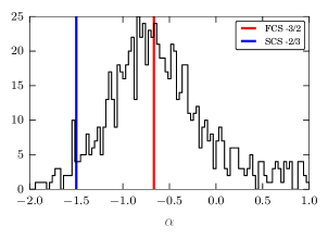
Figure 1: The GBM spectral catalog’s $\alpha$ distribution (Goldstein et al., 2012) with the two standard LODs superimposed.

Such comparisons of Band’s $\alpha$ index to various models have been a primary focus of modeling in the field. The GRB spectral catalog shows a peak in the $\alpha$ distribution of $\sim-1$ and many models try to achieve this central value (Pe’er & Waxman, 2004; Pe’er & Zhang, 2006; Medvedev et al., 2007; Beloborodov, 2010; Daigne, Bošnjak & Dubus, 2011; Uhm & Zhang, 2014). Though, there is a substantial amount of spread in the $\alpha$ distribution and no one model has made predictions that can explain all observed values. Such predictions are essential if it is expected that there is a universal process that occurs in GRB jets. It may be that several types of emission processes are active and vary from burst to burst. However, the current lack of self-consistent simulations from progenitor to radiation production limit such a global assessment. Within the standard fireball model, it is very probable that several emission components can be present in the observed spectrum (Meszaros & Rees, 2000), in particular emission from the photosphere and optically-thin regions could be superimposed upon one another.

Recently, a trend has therefore evolved with the possibility of reconciling synchrotron emission with the Band $\alpha$ distribution which consists of fitting a blackbody (non-dissipative photosphere) in combination with the typically fitted Band function to spectra observed by GBM (Guiriec et al., 2011; Axelsson et al., 2012; Iyyani et al., 2013; Preece et al., 2014). This is a natural continuation of the fitting of a blackbody and a power law that occurred during the BATSE era (Ryde, 2004, 2005; Ryde & Pe’er, 2009) however, with the expanded high-energy bandpass of GBM, the Band function and blackbody appear to be a more correct picture according to the data. The addition of the blackbody in some cases can change the $\alpha$ that was obtained by fitting the Band function alone to a value that is closer to what is expected from synchrotron. This is not, however, a universal observation (for example, see the $\alpha$ values from Axelsson et al., 2012). Still, the changing of $\alpha$ values has the potential to alleviate the problem of the LOD by implying that the measured values of $\alpha$ from Band only fits are actually incorrect measurements and the spectral data should be fitted with a Band+blackbody model which will infer that the emission is actually a combination of synchrotron and a blackbody.

There do exist predictions of emission coming from GRBs that have this non-thermal+blackbody spectrum which sufficiently motivates the fitting of Band+blackbody (Meszaros & Rees, 2000; Daigne & Mochkovitch, 2002). The significance of the observed blackbody has been calculated in many spectra (e.g. Axelsson et al., 2012) and been shown to be quite high. It is also possible that the blackbody found in the spectra could arise from summing together the evolving spectrum of a single non-thermal emission mechanism. Burgess & Ryde (2014) showed that it is possible for an evolving Band function to introduce a blackbody into spectral fits if too long of a duration of the evolution is summed together in the fit and that time-resolved analysis is required to check for the existence of a blackbody in the spectral data. However, in any case, it is important ask what a spectrum that consists of either fast or slow-cooling synchrotron that has been folded through the GBM response looks like when fitted by the Band function.

Herein, we investigate what the shape of the fitted Band function is when the intrinsic spectra consist of either fast or slow cooled synchrotron both with and without a blackbody by sythesizing these photon spectra and folding them through the GBM detector response and then fitting them with both Band and Band+blackbody photon functions. We are not primarily concerned about the quality of the fits but rather if the parameter distributions and values obtained from Band fits to actual physical photon models coincide with our assumptions. The article is divided as follows: in Section 2 we simulate fast and slow-cooling synchrotron with $\nu F_{\nu}$ peaks sampled from the GBM peak flux catalog (Goldstein et al., 2012) to investigate the effect that the detector bandpass has on measuring the low-energy index of the synchrotron spectrum. In Section 3 we simulate synchrotron spectra along with a blackbody where the synchrotron is held fixed and the blackbody flux is varied in $kT$ and flux to examine what the derived $\alpha$’s from Band fits would be under different scenarios.

We stress that we are not addressing whether or not synchrotron and synchrotron+blackbody can arise in the GRB spectra from physical principles. Rather, we are testing the assertions that the parameter distributions from Band and Band+blackbody fits can be directly used to infer conclusions on the various underlying emission scenarios at work in GRB outflows.

2 Testing the “line-of-death”

While the LOD is a strong motivator for model development in the field of GRBs, it has not been tested directly by actually simulating what the GRB spectral catalogs would look like if the spectra observed actually came from either FCS or SCS emission. What we aim to test is how the bandpass of the detector affects the measured Band $\alpha$ for the synchrotron models. Since the Band function’s curvature around the $\nu F_{\nu}$ peak differs from synchrotron and the synchrotron function curves continuously below the $\nu F_{\nu}$ peak, then it is likely that fitting a Band function to these physical spectra will have an effect on $\alpha$ as the $\nu F_{\nu}$ peak approaches the low-energy edge of the instrument’s bandpass.

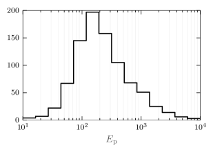
Figure 2: The GBM catalog $E_{\rm p}$ distribution.

To examine this question, we sample the $E_{\rm p}$ distribution (see Figure 2) of the $\it Fermi$ Gamma-ray Burst Monitor (GBM) peak flux catalog (Goldstein et al., 2012) and use those values to simulate synchrotron emission from fast- and slow-cooling electron distributions (see Equations 1 and 2). For SCS, we assume that the electrons are distributed as a power law in energy such that

$$n_{\rm e}^{\rm slow}(\gamma)\propto\gamma^{-p}\;:\;\gamma_{\rm min}\leq\gamma$$ (1)

where $p$ is the electron spectral index and $\gamma_{\rm min}$ is the injection energy of the process that accelerates the electrons. The spectrum of FCS arises when the electrons in the power law have cooled quickly compared to the dynamical timescale via synchrotron emission and pile up below the injection energy. This forms a broken power law distribution of the electrons in energy of the form

$$n_{\rm e}^{\rm fast}(\gamma)\propto\left\{\begin{array}[]{ll}\gamma^{-2}&:\;\gamma_{\rm cool}<\gamma\leq\gamma_{\rm min}\\ \gamma^{1-p}&:\;\gamma<\gamma_{\rm min}\end{array}\right.$$ (2)

where $\gamma_{\rm cool}$ is the energy to which the electrons cool after a characteristic cooling time (for a review on synchrotron cooling see Sari, Piran & Narayan, 1998; Burgess et al., 2014). To compute the synchrotron emission from these electron distributions, we convolve them with the standard synchrotron kernel (Blumenthal & Gould, 1970). For each sampled $E_{\rm p}$ from the GBM catalog, we use the relation $E_{\rm p}\propto\Gamma B\gamma_{\rm min}^{2}$, where $\Gamma$ and $B$ are the bulk Lorentz factor and magnetic field strength respectively, to scale the $\nu F_{\nu}$ peak of the synchrotron spectrum. For the electron index, $p$ we assume $p=3.5$ for slow-cooling and $p=2.5$ for fast-cooling to recover the average observed value of the Band function’s high-energy index, $\beta\sim-2.2$.

With the derived photon spectra, we use detector responses from GBM to produce count spectra for two Sodium-Iodide (NaI) and one Bismuth-Germanante (BGO) detectors. Each simulated source spectrum has a synthetic background added such that the signal-to-noise ratio is 30. The photon distribution of the background spectrum is a decreasing power law in energy. In total, 1000 spectra are created for each of the SCS and FCS models and then they are fit with the Band function and their parameters recorded.

Examining the distribution of $\alpha$’s found by simulating SCS, it is clear that only a small portion of GBM spectra can be explained by the model. We note that the LOD is actually worse than what was derived in (Crider et al., 1998; Preece et al., 1998) because the SCS $\alpha$ distribution peaks at $\sim-.8$ as shown in Figure 3. This leaves the harder half of the GBM distribution unreachable. The tail of the distribution stretches towards more negative values. The spread in the values of $\alpha$ derived from the Band fits to the SCS and FCS synthetic spectra is attributed to the different values of $E_{\rm p}$ alone as can be seen in Figure 4. For the distribution of $\alpha$’s from FCS, the LOD at $-3/2$ holds true and the width of the distribution is narrow and stretches towards negative values. This is because the FCS is very broad and its asymptotic power law behavior is well approximated by a Band fit at low energies. Clearly, the two standard synchrotron emission scenarios cannot account for the GBM spectral catalog’s $\alpha$ distribution.

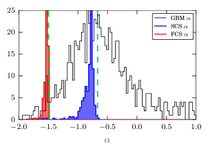
Figure 3: The $\alpha$ distributions of the GBM peak flux spectral catalog with the $\alpha$ distributions from fast- and slow-cooling synchrotron superimposed. The green lines indicate the LODs.

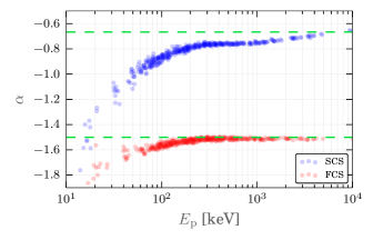
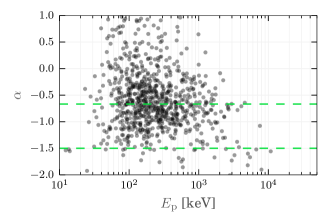
Figure 4: $E_{\rm p}$ and $\alpha$ correlation for the FCS and SCS simulations. The left panel demonstrates how the FCS (red) and SCS (blue) models would have $\alpha$ measured if they were the intrinsic spectra. The right panel is the actual GBM spectral catalog $E_{\rm p}$-$\alpha$ correlation. In both panels, the LODs are shown by the green lines.

Preece et al. (1998) assumed the low-energy data was poorly described by $\alpha$ because the Band function did not always approach their asymptotic power law behavior if $E_{\rm p}$ was too close to the low-energy bandpass of the detector. Therefore, they used the tangent slope of the Band function at some fiducial value near the window to define an effective power law slope ($\alpha_{\rm eff}$) that the authors claimed was a better measure of the low-energy behavior of the data. This is however, not what we are testing herein and the correlation observed in Figure 4 is due to spectral curvature. We are testing how the Band function fit is affected by the fact that synchrotron has a broader curvature than Band and this will be sampled differently when the $\nu F_{\nu}$ peak of the spectrum is near the low-energy bandpass of the detector.

Nevertheless, the effect in Preece et al. (1998) could play an important role in determining the low-energy behavior of the data. We therefore test the ability of Band function fits to measure this behavior. We simulate a Band function with $E_{\rm p}\in\left\{20;1000\right\}$ keV with $\alpha=-1$ and $\beta=-2.2$ and then fit them with the Band function. We find that the $\alpha$ of the data is recovered from the data regardless of the value of $E_{\rm p}$ (see Figure 5). Moreover, were we to use $\alpha_{\rm eff}$, we would artificially soften the spectrum. Therefore, we concluded that the Band function’s natural $\alpha$ value is a appropriate to use for our purposes.

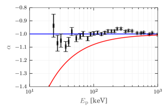
Figure 5: The effect of $E_{\rm p}$ being close to the low-energy bandpass on $\alpha$ is demonstrated. The simulated value of $\alpha$ is shown in blue and the recovered values from Band fits are shown in black. The $\alpha_{\rm eff}$ curve introduced in Preece et al. (1998) is shown in red. It clearly would artificially soften the correctly recovered $\alpha$.

3 Can a blackbody fix the “line-of-death”?

The spectrum of a blackbody is uniquely set apart among astrophysical emissivities by having a hard low-energy slope and the narrowest $\nu F_{\nu}$ peak. Regardless of the physical implications of having emission from GRBs in the form of synchrotron+blackbody, the addition of a blackbody below the $\nu F_{\nu}$ peak of synchrotron affords the opportunity to explain the harder values of $\alpha$ in the GBM spectral catalog. There are reasons to take caution with using the value of $\alpha$ to infer a emission mechanism. Burgess et al. (2014), for example, showed that even if $\alpha$ from a Band fit to real GRB data has a value that corresponds to FCS emission, a FCS photon model cannot fit the data because the data around the $\nu F_{\nu}$ peak are too narrow for the broad curvature of FCS. The point being that the curvature of the spectrum is as important as the values of its asymptotic power law indices.

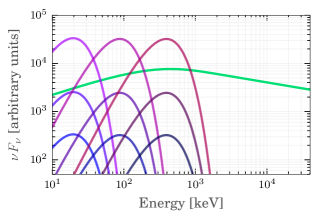
Figure 6: Demonstrating the grid of synthesized blackbodies (blue to purple) with FCS (green) superimposed.

With curvature in mind, it is important to assess not only how adding a blackbody component to the synchrotron would affect the $\alpha$ of a Band fit to both components combined, but also whether or not the combined curvature of the two components can be fit by the much narrower curvature of the Band function. This is essential to understanding if the model of synchrotron+blackbody can account for the observed spectra. To investigate this problem, we simulate both FCS and SCS held at a constant $E_{\rm p}$ and then add on a blackbody in a grid of the blackbody temperature, $kT$ and the ratio of blackbody energy flux ($F_{\rm BB}$) to total energy flux ($F_{\rm tot}$) defined such that when $R\equiv F_{\rm BB}/F_{\rm tot}=1$, the blackbody accounts for the entire flux of the spectrum. The grid of both $kT\in\{5;100\}$ keV and $R\in\{0.01;0.5\}$ (see Figure 6) span ranges that more than cover what has been observed in the data (Guiriec et al., 2011; Axelsson et al., 2012; Iyyani et al., 2013; Burgess et al., 2014). For each grid of blackbody parameters and each of the synchrotron models we pick two values of fixed $E_{\rm p}$ for the synthesized synchrotron photon spectra: $E_{\rm p}=300$ keV that represents the average observed value in the data and $E_{\rm p}=1$ MeV to examine in greater detail what happens below the $\nu F_{\nu}$ peak when a blackbody is added. In total, there are four grids each with 900 synthetic spectra for all variations of the blackbody parameters.

3.1 Synthetic Slow-cooling Synchrotron + Blackbody

Due to its prolific use as an inference parameter for emission models, we first examine the value of $\alpha$ obtained from Band only fits to the synchrotron+blackbody simulations. Figure 7a and Figure 8a show the behavior of $\alpha$ as a function of the blackbody parameters ($R$, $kT$) for $E_{\rm p}=300$ keV and $1$ MeV respectively. For this grid, it is obvious that obtaining values of $\alpha\geq 0$ requires low temperature blackbodies that must account for a substantial fraction of the total energy flux. The key change between the two values of simulated synchrotron $E_{\rm p}$ is that the harder values of $\alpha$ are achieved for lower $R$ and higher $kT$ when $E_{\rm p}$ is greater.

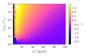
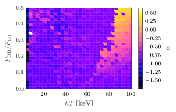
Figure 7: The $\alpha$ distribtuions from the fits of Band (left) and Band+blackbody (right) to SCS+blackbody simulations with $E_{\rm p}=300$ keV.

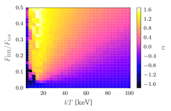
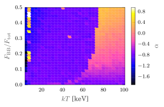
Figure 8: Same as Figure 7 but with $E_{\rm p}=1$ MeV.

Figure 7b and Figure 8b demonstrate the behavior of $\alpha$ when the Band+blackbody model is fit the simulated spectra. As expected, the value of $\alpha$ shifts to a more SCS-like (-2/3) value except for high values of $kT$ due to the fact that at high $kT$, the blackbody $\nu F_{\nu}$ peak coincides with synchrotron peak. This makes it very hard for the fitting engine to fit both components at their simulated values and lowers the value of $kT$ while increasing the value of $\alpha$, i.e., if a true blackbody in the data has a temperature that causes its $\nu F_{\nu}$ peak to coincide with the peak of synchrotron (or perhaps any other non-thermal emissivity), it is unlikely that a Band+blackbody fit will find values that are indicative of the actual physical spectrum (see Figures 9 and 10).

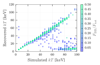
Figure 9: The simulated $kT$ of the blackbody vs. the $kT$ recovered when the spectrum is fitted by Band+blackbody when the simulated non-thermal spectrum is SCS with an $E_{\rm p}=300$ keV.

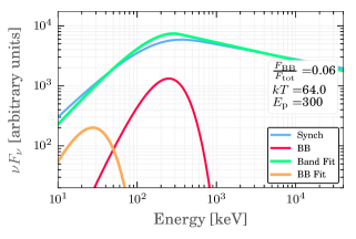
Figure 10: An example spectrum demonstrating the difference in the simulated blackbody and the one recovered in a Band+blackbody fit when the blackbody $\nu F_{\nu}$ peak coincides with the synchrotron $\nu F_{\nu}$ peak.

To understand how the combined curvature of the simulated SCS+blackbody spectrum affects the fit of Band only to the data, we examine how the high-energy power law index of the Band function ($\beta$) is affected by the addition of the blackbody. Figure 11 shows the recovered value of $\beta$ for the different blackbody parameters. Very hard values ($\beta\geq-2.$) are found for values of the blackbody typically observed in the data ($kT\simeq 30$ keV and $R\simeq 0.1$). This is due to the broad curvature of the SCS+blackbody spectrum that cannot be fit with the narrower Band function. To compensate, the Band function $E_{\rm p}$ is lowered and $\beta$ increased (see Figure 12). Such values of $\beta$ are rare in the spectral catalog (see Figure 13).

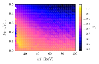
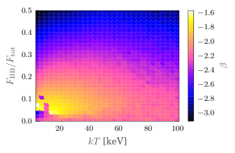
Figure 11: The values of $\beta$ recovered for the different blackbody parameters with $E_{\rm p}=300$ keV (left) and $E_{\rm p}=1$MeV (right).

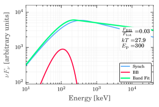
Figure 12: An example spectrum demonstrating the Band function’s inability to properly fit the broad curvature of the simulated SCS+blackbody spectrum. The Band function adjusts by lowering $E_{\rm p}$ and increasing $\beta$ to values not typically found in the GBM catalog.

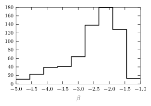
Figure 13: The GBM catalog $\beta$ distribution.

Finally, the behavior of $E_{\rm p}$ is examined. When fitting Band only to the synthetic spectra where the synchrotron $E_{\rm p}=300$ keV, Figure 14a shows the Band $E_{\rm p}$ is sensitive to the blackbody $kT$ except when $R$ is very low. However, when the synchrotron $E_{\rm p}$ is increased to 1 MeV, Figure 14b shows the recovered Band $E_{\rm p}$ to be sensitive to $kT$ nearly independent of $R$. Next, the shift in the Band $E_{\rm p}$ when the Band+blackbody model is fitted appears to be more correlated with $kT$ than $R$ (see Figurea 15 and 16). For lower values of $kT$ (similar to values recovered in the real observations) $E_{\rm p}$ shifts systematically to lower values while for high values of $kT$, the shift of $E_{\rm p}$ is to higher values. It is important to notice that for both low and high $kT$ the value of $E_{\rm p}$ recovered by the Band+blackbody fit is not always accurate and can vary greatly from the simulated values.

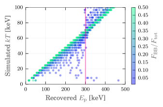
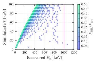
Figure 14: The value of the recovered Band $E_{\rm p}$ as a function of the simulated blackbody $kT$ when the simulated SCS spectrum has an $E_{\rm p}=300$ keV (left) and $E_{\rm p}=1$ MeV (right). The pink line indicates the simulated value of the synchrotron $E_{\rm p}$.

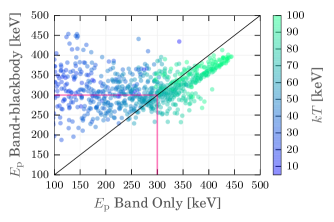
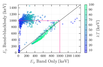
Figure 15: The shift in recovered $E_{\rm p}$ as a function of $kT$ when fitting Band+blackbody to the SCS+blackbody simulations when the simulated SCS spectrum has an $E_{\rm p}=300$ keV (left) and $E_{\rm p}=1$ MeV (right). The pink lines indicate the simulated value of the synchrotron $E_{\rm p}$. Points above the black line shift to higher $E_{\rm p}$ values when fit with Band+blackbody as opposed to Band.

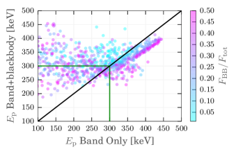
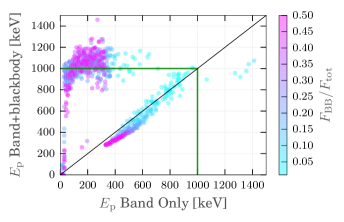
Figure 16: Same as Figure 15 but showing how the $E_{\rm p}$ shift is affected by $R$. The green lines indicate the simulated value of the synchrotron $E_{\rm p}$.

3.2 Synthetic Fast-cooling Synchrotron + Blackbody

The FCS+blackbody simulations exhibit many of the same features found for SCS with minor adjustments for the values of $\alpha$ found in the Band only fits with respect to the simulated blackbody parameters (see Figures 17 and 18). As with SCS, achieving values of $\alpha>-0.8$ requires $kT\lesssim 60$ keV and $R\gtrsim.1$, which does not coincide with observations of blackbodies in GRB spectra. However, when the spectra are fit with the Band+blackbody model, the measured $\alpha$ shifts to what is expected for FCS unless the blackbody $\nu F_{\nu}$ peak coincides with the FCS $E_{\rm p}$. This can be seen just as with SCS via Figure 19 and 20.

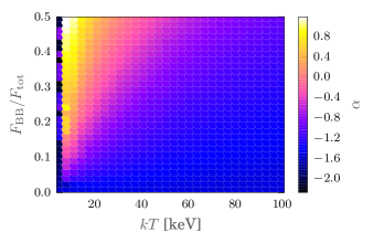
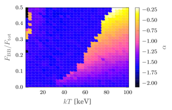
Figure 17: The $\alpha$ distribtuions from the fits of Band (left) and Band+blackbody (right) to FCS+blackbody simulations with $E_{\rm p}=300$ keV.

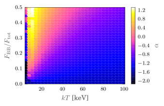
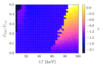
Figure 18: Same as Figure 17 but with $E_{\rm p}=1$ MeV.

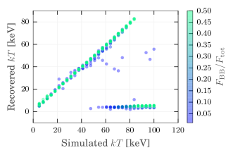
Figure 19: The simulated $kT$ of the blackbody vs. the $kT$ recovered when the spectrum is fitted by Band+blackbody when the simulated non-thermal spectrum is FCS with an $E_{\rm p}=1$ MeV.

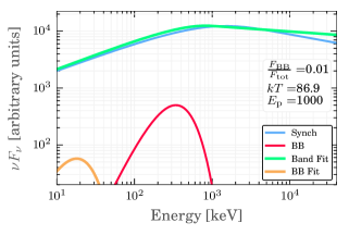
Figure 20: An example spectrum demonstrating the difference in the simulated blackbody and the one recovered in a Band+blackbody fit when the blackbody $\nu F_{\nu}$ peak coincides with the synchrotron $\nu F_{\nu}$ peak.

The behavior of the recovered value of $\beta$ from the simulations is slightly altered from what is observed with SCS+blackbody as shown in Figures 21 and 22. Whereas high $kT$ and low $R$ result in acceptable $\beta$ values for SCS+blackbody, the value of $\beta$ for FCS+blackbody is mostly sensitive to $R$. The already broad curvature of FCS is not affected so much by where the blackbody $\nu F_{\nu}$ peak appears in energy as it is affected by the blackbody’s flux. Still, the curvature is too wide for the Band function to fit the spectrum without increasing $\beta$ to typically unobserved, higher values.

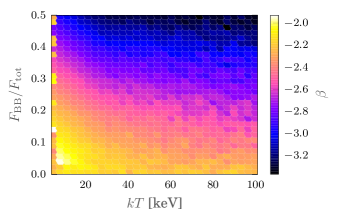
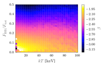
Figure 21: The values of $\beta$ recovered for the different blackbody parameters with $E_{\rm p}=300$ keV (left) and $E_{\rm p}=1$MeV (right). The pink line indicates the simulated value of the synchrotron $E_{\rm p}$.

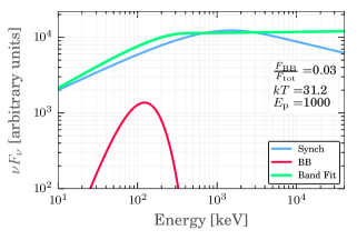
Figure 22: An example spectrum demonstrating the Band function’s inability to properly fit the broad curvature of the simulated FCS+blackbody spectrum. The Band function adjust by lowering $E_{\rm p}$ and increasing $\beta$ to values not typically found in the GBM catalog.

The value of $E_{\rm p}$ from Band only fits is always affected by the $kT$ regardless of the flux of the blackbody as is shown in Figure 23. Again, this is an effect of the broad curvature of the FCS spectrum. Figures 24 and 25 show a similar behavior as with SCS for the shift in the recovered $E_{\rm p}$ when fitting with Band or Band+blackbody but is slightly more sensitive to the flux of the simulated blackbody though the overall dependence is still from changing $kT$.

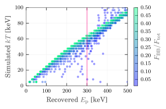
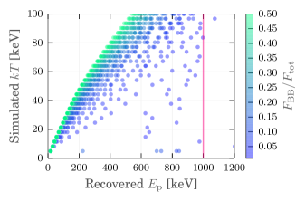
Figure 23: The value of the recovered Band $E_{\rm p}$ as a function of the simulated blackbody $kT$ when the simulated FCS spectrum has an $E_{\rm p}=300$ keV (left) and $E_{\rm p}=1$ MeV (right). The pink line indicates the simulated value of the synchrotron $E_{\rm p}$.

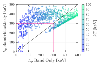
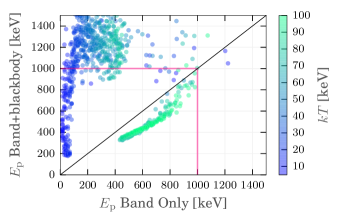
Figure 24: The shift in recovered $E_{\rm p}$ as a function of $kT$ when fitting Band+blackbody to the FCS+blackbody simulations when the simulated SCS spectrum has an $E_{\rm p}=300$ keV (left) and $E_{\rm p}=1$ MeV (right). The pink line indicates the simulated value of the synchrotron $E_{\rm p}$. Points above the black line shift to higher $E_{\rm p}$ values when fit with Band+blackbody as opposed to Band.

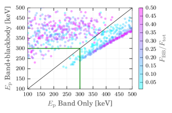
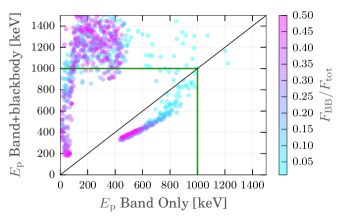
Figure 25: Same as Figure 24 but showing how the $E_{\rm p}$ shift is affected by $R$. The green line indicates the simulated value of the synchrotron $E_{\rm p}$.

Overall, we find similar behaviors for the fits of Band and Band+blackbody to the simulated SCS and FCS photons models. The main change occurs in the values of $\alpha$ and $\beta$ recovered as a function of the blackbody parameters. The relationships found in the test all have similar dependencies with the magnitudes of the effect changed due to the different curvature of the SCS and FCS spectra.

4 Discussion

Herein, we have investigated the ability of both optically-thin synchrotron emission in the form of slow-cooling and fast-cooling as well as synchrotron emission with an additional blackbody (photosphere) to explain the observed Band parameter distributions in the GBM spectral catalogs. Additionally, we have investigated in detail the properties one would observe if the true observed spectrum is synchrotron+blackbody and is fit with a Band+blackbody photon model. We confirm the original conclusion of Crider et al. (1998); Preece et al. (1998) that neither SCS or FCS alone can explain the entire catalogs. Moreover, we find that if the true observed spectrum is SCS then the “line-of-death” should actually be at $\alpha_{\rm LOD}\simeq-0.8$ rather than the originally stated -2/3 owing to the fact that synchrotron asymptotically approaches a power law shape and continuously curves below its $\nu F_{\nu}$ peak. This causes a fit with the Band function to recover an $\alpha$ that is dependent on the location of the $\nu F_{\nu}$ peak with respect to the GBM low energy bandpass. Furthermore, we conclude that it is difficult to recover the parameter distributions of the GBM spectral catalog by adding on a blackbody to synchrotron emission if past fits to observations represent an actual sample of the typical blackbody parameters. If GBM observations typically contain a blackbody with $kT\simeq 30$ keV and $R\simeq 0.1$ then values of $\alpha>-2/3$ would not be found when fitting these spectra with a Band function alone. Also, much harder values of Band’s $\beta$ would be observed for the typically found parameters of the blackbody. This is due to the broad total curvature introduced by the combined synchrotron+blackbody spectrum which is too broad for the narrower Band function to fit.

To explain the hardest $\alpha$-values in the catalog, we need to observe blackbodies with a higher value of $R$ and the blackbody would dominate the spectrum unlike what is observed. This finding indicates that while fits to these GBM spectra with Band+blackbody are to be statistically better descriptions of the data, the resulting Band function is very different from a synchrotron function ($\alpha$ too hard and the spectral width is too narrow.) We have checked the preliminary GBM time-resolved spectral catalog (Yu et al., 2014a) for spectra with hard $\alpha$ and $\beta$ which these simulations indicate could contain a bright blackbody component. However, out of $\sim 1800$ spectra, very few have both hard $\alpha$ and $\beta$ and those that do contain no statistically significant blackbody.

The $E_{\rm p}$ recovered from the Band+blackbody fits to the multicomponent simulations is not always accurate and can differ from the simulated true value. This, combined with the fact that the fitted flux and $kT$ of the blackbody in these synthetic data are not always accurate means that using the fitted Band function $E_{\rm p}$ in multicomponent fits to infer properties about the GRB or to examine flux-luminosity relations should be done with caution. The Band function is simply too flexible and the free parameters work together to fit the curvature of the data in the best way possible without regard for physics.

There are other forms of synchrotron emission and processes that can result in different spectral shapes. For example, Klein-Nishina losses can significantly alter the low-energy spectrum of synchrotron emission (Daigne, Bošnjak & Dubus, 2011). Additionally, Uhm & Zhang (2014) have shown that altering the magnetic field structure along the radial direction of the outflow can also modify the low-energy slope. However, it is not clear if these processes alter the spectral curvature of synchrotron resulting in a narrower $\nu F_{\nu}$ peak more consistent with the Band function. If that is the case, then it is possible that the combination of this narrower synchrotron emission produced in Poynting flux jets (Giannios & Spruit, 2004; Zhang & Yan, 2011) and a blackbody could explain the GBM catalog; therefore, such emission mechanism should be tested in a similar way as what is done here (see however Bégué & Pe’er, 2014, where a problem with Poynting flux jets and photospheric emission is discussed).

One should also note that the few studies that have attempted to numerically simulate spectra composed of synchrotron emission and a photospheric blackbody. For example, Hascoet, Daigne & Mochkovitch (2013); Gao & Zhang (2014) use the Band function with an $\alpha=-3/2$ as a proxy for the actual synchrotron emission. This artificially imposes a narrower curvature on the simulated spectra and guarantees that the spectra will mimic the shape observed in the data. It will therefore be difficult to use these simulations to assess the physical validity of Band+blackbody fits to observed data. However, when these simulations advance to the point that both the thermal and non-thermal components are realistic physical representations of the theorized emission, a similar assessment to what is done here can proceed.

Studies where a physical synchrotron photon model is used to replace the Band function in spectral fits have shown that it is possible to fit some GRB spectra with synchrotron or synchrotron+blackbody (Burgess et al., 2014; Yu et al., 2014b). However, these works find that only SCS can fit the data accurately due mainly to the curvature of the data around the $\nu F_{\nu}$ peak. However, calling these spectra SCS could be misleading. Beniamini & Piran (2013) point out that when $\gamma_{\min}$ and $\gamma_{\rm cool}$ are close to each other, the electron distribution is in a marginally fast-cooling state but still mimics the shape of SCS. Additionally, the narrowness of the $\nu F_{\nu}$ peak in the data can be fit with thermal emissivities related to sub-photospheric dissipation (Iyyani & Ryde, 2014). All of these findings indicate that spectral curvature must be considered when trying to infer physics from fits to GRB spectra. There is a tendency in theoretical modeling to aim for a single value of $\alpha$ as a mark of success in explaining the emission process in GRBs. Obviously, as we have shown, many factors such as curvature, detector bandpass, and the limited shape of the Band function should be considered as well as the peak of the $\alpha$ distribution when assessing the predictive power of a model. Beloborodov (2013) points out that synchrotron faces a problem of more than just the LOD. One must consider the narrowness of the $\nu F_{\nu}$ peak and the clustering of $E_{\rm p}$ which is not easily reconciled with the current knowledge of electron acceleration processes and astrophysical magnetic fields. In fact, Axelsson et al. (2014) study the width of spectral curvature in the GBM catalogs and find that nearly half of the spectra are far too narrow to be explained by synchrotron emission. It is possible that this corresponds to our finding that only half of $\alpha$ distribution can be explained by synchrotron or synchrotron+blackbody.

In conclusion, optically-thin synchrotron emission with or without a blackbody accounting for emission from a non-dissipative photosphere is insufficient to explain the entire GBM spectral catalog. Both scenarios can account for little more than half the observed spectra. This implies that at least a large fraction of the catalog GRBs have another origin such as emission from the photosphere including subphotospheric-dissipation (Rees & Meszaros, 2005; Pe’er, Meszaros & Rees, 2005; Beloborodov, 2010) and structured jets Goodman (1986); Lundman, Pe’er & Ryde (2014).

References

- Axelsson et al. (2012) Axelsson M. et al., 2012, ApJL, 757, L31
- Axelsson et al. (2014) Axelsson M., et al., 2014, In preparartion
- Band, Matteson & Ford (1993) Band D., Matteson J., Ford L., 1993, ApJ, 413, 281
- Baring & Braby (2004) Baring M. G., Braby M., 2004, ApJ
- Bégué & Pe’er (2014) Bégué D., Pe’er A., 2014, preprint (arXiv:1410.2730)
- Beloborodov (2010) Beloborodov A. M., 2010, MNRAS, 407, 1033
- Beloborodov (2013) Beloborodov A. M., 2013, ApJ, 764, 157
- Beniamini & Piran (2013) Beniamini P., Piran T., 2013, ApJ, 769, 69
- Blumenthal & Gould (1970) Blumenthal G. R., Gould R. J., 1970, Reviews of Modern Physics
- Burgess et al. (2014) Burgess J. M. et al., 2014, ApJ, 784, 17
- Burgess & Ryde (2014) Burgess J. M., Ryde F., 2014, submitted
- Chevalier & Li (1999) Chevalier R. A., Li Z.-Y., 1999, ApJL, 520, L29
- Crider et al. (1998) Crider A., Liang E. P., Preece R. D., Briggs M. S., Pendleton G. N., Paciesas W. S., Band D. L., Matteson J. L., 1998, American Astronomical Society, 193, 1380
- Daigne, Bošnjak & Dubus (2011) Daigne F., Bošnjak Ž., Dubus G., 2011, A&A, 526, 110
- Daigne & Mochkovitch (2002) Daigne F., Mochkovitch R., 2002, MNRAS, 336, 1271
- Gao & Zhang (2014) Gao H., Zhang B., 2014, preprint (arXiv:1409.3584)
- Ghirlanda, Celotti & Ghisellini (2003) Ghirlanda G., Celotti A., Ghisellini G., 2003, A&A, 406, 879
- Giannios & Spruit (2004) Giannios D., Spruit H., 2004, A&AS
- Goldstein et al. (2012) Goldstein A. et al., 2012, ApJS, 199, 19
- Goodman (1986) Goodman J., 1986, ApJ, 308, L47
- Guiriec et al. (2011) Guiriec S. et al., 2011, ApJL, 727, L33
- Hascoet, Daigne & Mochkovitch (2013) Hascoet R., Daigne F., Mochkovitch R., 2013, A&A, 551, 124
- Iyyani & Ryde (2014) Iyyani S., Ryde F., 2014, In preperation
- Iyyani et al. (2013) Iyyani S. et al., 2013, MNRAS, 433, 2739
- Kaneko et al. (2006) Kaneko Y., Preece R. D., Briggs M. S., Paciesas W. S., Meegan C. A., Band D. L., 2006, ApJS, 166, 298
- Lundman, Pe’er & Ryde (2014) Lundman C., Pe’er A., Ryde F., 2014, MNRAS, 440, 3292
- Medvedev et al. (2007) Medvedev M., Lazzati D., Morsony B., Workman J., 2007, ApJ, 666, 339
- Meszaros & Rees (2000) Meszaros P., Rees M. J., 2000, ApJ, 530, 292
- Meszaros & Rees (2010) Meszaros P., Rees M. J., 2010, ApJ, 715, 967
- Pe’er, Meszaros & Rees (2005) Pe’er A., Meszaros P., Rees M. J., 2005, ApJ
- Pe’er & Waxman (2004) Pe’er A., Waxman E., 2004, ApJ, 613, 448
- Pe’er & Zhang (2006) Pe’er A., Zhang B., 2006, ApJ, 653, 454
- Preece et al. (2014) Preece R. et al., 2014, Science, 343, 51
- Preece et al. (1998) Preece R. D., Briggs M. S., Mallozzi R. S., Pendleton G. N., Paciesas W. S., Band D. L., 1998, ApJ, 506, L23
- Ramirez-Ruiz, Lazzati & Blain (2002) Ramirez-Ruiz E., Lazzati D., Blain A. W., 2002, ApJL, 565, L9
- Rees & Meszaros (2005) Rees M. J., Meszaros P., 2005, ApJ, 628, 847
- Ryde (2004) Ryde F., 2004, ApJ, 614, 827
- Ryde (2005) Ryde F., 2005, ApJL, 625, L95
- Ryde & Pe’er (2009) Ryde F., Pe’er A., 2009, ApJ, 702, 1211
- Sari, Piran & Narayan (1998) Sari R., Piran T., Narayan R., 1998, ApJL, 497, L17
- Uhm & Zhang (2014) Uhm Z. L., Zhang B., 2014, Nature, 10, 351
- Woosley & Heger (2006) Woosley S. E., Heger A., 2006, ApJ, 637, 914
- Yu et al. (2014a) Yu H. F., et al., 2014a, In preparartion
- Yu et al. (2014b) Yu H. F., et al., 2014b, A&A, in press
- Zhang & Yan (2011) Zhang B., Yan H., 2011, ApJ, 726, 90