Quantization conditions and functional equations in ABJ(M) theories

Abstract

The partition function of ABJ(M) theories on the three-sphere can be regarded as the canonical partition function of an ideal Fermi gas with a non-trivial Hamiltonian. We propose an exact expression for the spectral determinant of this Hamiltonian, which generalizes recent results obtained in the maximally supersymmetric case. As a consequence, we find an exact WKB quantization condition determining the spectrum which is in agreement with numerical results. In addition, we investigate the factorization properties and functional equations for our conjectured spectral determinants. These functional equations relate the spectral determinants of ABJ theories with consecutive ranks of gauge groups but the same Chern-Simons coupling.

1 Introduction

In the last years, there has been a lot of progress in understanding ABJ(M) theory abjm ; abj . In kwy the partition function of ABJ(M) theory on the three-sphere was reduced to a matrix integral which turned out to be closely related to topological strings on local $\mathbb{P}^{1}\times\mathbb{P}^{1}$ mpabjm . In dmp the connection with topological strings was used to compute recursively the full ’t Hooft $1/N$ expansion, which by the AdS/CFT correspondence corresponds to the genus expansion of a dual type IIA superstring theory. In order to understand the M-theory lifting of this result, one has to study ABJM theory in a different regime, usually called the M-theory regime or M-theory expansion, in which $N$ is large but the coupling constant is fixed. The study of the matrix models computing partition functions of Chern–Simons–matter theories in the M-theory regime was initiated in hkpt , where the strict large $N$ limit was solved for a large class of theories.

In mp , a different approach was proposed to study the M-theory regime of ABJM theory and related models. In this approach, the partition function of ABJ(M) is interpreted as the partition function of an ideal Fermi gas. The M-theory limit corresponds to the thermodynamic limit of this gas, and the coupling constant of ABJM theory becomes Planck’s constant. The Fermi gas formulation of ABJM theory has been intensively studied in mp ; hmo ; py ; hmo2 ; cm ; hmo3 ; hmmo , leading to an exact expression for the the partition function of ABJ(M) theory which resums the ’t Hooft expansion and includes as well non-perturbative, large $N$ instanton corrections dmpnp .

An important aspect of the Fermi gas approach is that, since we are dealing with an ideal gas, all the physics of the problem is encoded in the spectrum of the one-particle Hamiltonian. Therefore one should be able to reproduce the results of hmmo by studying the spectral problem associated to the Fermi gas of ABJ(M) theory. Conversely, the exact expression for the partition function should encode all the information about the spectrum of the Fermi gas. In km ; kallen , a WKB quantization condition for ABJ(M) theory has been proposed by studying the relation between the spectrum of the Hamiltonian and the thermodynamics of the Fermi gas. This condition turns out to be exact in the cases in which the theory has maximal supersymmetry cgm , but it needs additional corrections in the general case, as it was recently pointed out in huang (see also hw ) by a detailed numerical analysis.

One of the key results of cgm is that, in the maximally supersymmetric cases, one can write an explicit expression for the grand canonical partition function of the Fermi gas, which is nothing but the spectral determinant of the Hamiltonian. This expression involves a Jacobi theta function, and the spectrum can be read from the vanishing locus of this theta function. In this paper we generalize the results of cgm to ABJ(M) theories with ${\cal N}=6$ supersymmetry. We write a general formula for the spectral determinant of these theories, which involves now a generalization of the theta function. In particular, we derive an exact WKB quantization condition for the spectrum. The quantization condition proposed in km ; kallen is only an approximation to the exact quantization condition, and in general it receives corrections that we can compute analytically in this paper. Our general result explains why the quantization conditions of km ; kallen are valid in the maximally supersymmetric cases. It reproduces the corrections found numerically in the case of ABJM theory in huang , and we also test these corrections in detail against explicit calculations of the spectrum in both ABJM theory and ABJ theory.

As it was emphasized in the companion paper ghm , where we studied the implications of these ideas for topological string theory, the quantization condition is obtained as a corollary of a stronger result, namely a conjectural exact expression for the spectral determinant. This expression was tested in detail in cgm in the maximally supersymmetric case, where it was shown that it reproduces the values for the partition functions calculated in hmo ; py ; abj-moriyama ; honda-o . In the general case with ${\cal N}=6$ supersymmetry our conjecture for the spectral determinant is more difficult to verify, since this involves a resummation of the Gopakumar–Vafa expansion of the topological string free energy gv . However, we are able to perform this resummation in one special case (ABJM theory with $k=4$), and we obtain a generating functional for the partition functions of this theory in full agreement with existing calculations hmo2 .

In exactly solvable cases, spectral determinants enjoy very interesting properties. They can be factorized according to the parity of the eigenfunctions, and they satisfy functional equations (see for example voros ; dt ). In this paper, we initiate the study of such properties in the spectral problem of ABJ(M) theory. We find for example an explicit factorization of the spectral determinant in the maximally supersymmetric case $k=1$, as well as conjectural functional equations akin to those found in voros ; dt in Quantum Mechanics. These functional equations relate the spectral determinants of ABJ theories with consecutive ranks of gauge groups. In particular, if the Chern-Simons levels are odd, these equations determine all the ABJ spectral determinants from the ABJM ones via the Seiberg-like duality of ABJ theory abj .

This paper is organized as follows. In section 2 we review some general aspects of the Fermi gas formalism. In section 3 we introduce the spectral determinant and the generalized theta function associated to the ABJ(M) grand potential, and we deduce the exact quantization condition for the energy levels by looking at the zeros of this generalized theta function. We also give strong numerical evidence in support of our computations. In section 4 we study an example with $\mathcal{N}=6$ supersymmetry and we show that the full genus expansion can be resummed into an explicit function on the moduli space. In section 5 we discuss the factorization of the spectral determinant according to the parity of the energy levels and in section 6 we give evidence for some functional identities. In section 7 we draw some conclusions. There are also three appendices. In appendix A and B we give some details for computations appearing in section 4 and in section 5. In appendix C we explain the numerical technique used to compute the spectrum.

2 The Fermi gas approach to ABJ(M) Theory

The ABJ(M) theory abjm ; abj is an $\mathcal{N}=6$ superconformal Chern-Simons-matter theory with gauge group $U(N_{1})_{k}\times U(N_{2})_{-k}$. It consists in two Chern-Simons nodes, with couplings $k$ and $-k$, respectively, together with four hypermultiplets in the bifundamental representation. By using localization techniques it is possible to reduce the ABJ(M) partition function on $\mathbb{S}^{3}$ to the following matrix integral kwy :

$$Z(N_{1},N_{2},k)$$ (2.1)

$$={{\rm i}^{-\frac{1}{2}(N_{1}^{2}-N_{2}^{2})}\over N_{1}!N_{2}!}\int\prod_{i=1}^{N_{1}}{{\rm d}\mu_{i}\over 2\pi}\prod_{j=1}^{N_{2}}{{\rm d}\nu_{j}\over 2\pi}{\prod_{i<j}\left(2\sinh\left({\mu_{i}-\mu_{j}\over 2}\right)\right)^{2}\left(2\sinh\left({\nu_{i}-\nu_{j}\over 2}\right)\right)^{2}\over\prod_{i,j}\left(2\cosh\left({\mu_{i}-\nu_{j}\over 2}\right)\right)^{2}}{\rm e}^{-{{\rm i}k\over 4\pi}\left(\sum_{i}\mu_{i}^{2}-\sum_{j}\nu_{j}^{2}\right)}.$$

When $N_{1}=N_{2}=N$ the above matrix integral can be also written as kwytwo ; mp

$$Z(N,k)={1\over N!}\int\prod_{i=1}^{N}{{\rm d}x_{i}\over 4\pi k}{1\over 2\cosh{x_{i}\over 2}}\prod_{i<j}\left(\tanh\left({x_{i}-x_{j}\over 2k}\right)\right)^{2}.$$ (2.2)

These matrix integrals can be studied in the conventional ’t Hooft expansion mpabjm ; dmp . In mp it was pointed out that, to fully understand the non-perturbative effects, one has to go beyond the ’t Hooft $1/N$ expansion and study the M-theory regime of (2.1). In this regime, the ranks of the gauge groups are large but the coupling $k$ is fixed. To study this regime it is convenient to use the Fermi gas approach mp in which we rewrite the matrix integral as the canonical partition function of a one-dimensional ideal Fermi gas. In this approach, the Chern-Simons coupling $k$ plays the role of the Planck constant:

$$\hbar=2\pi k.$$ (2.3)

The Fermi gas formulation of the ABJ matrix integral was proposed in ahs ; honda where (2.1) was written as

$$Z(N,N+M,k)={\rm e}^{{\rm i}\vartheta(N,M,k)}Z_{\rm CS}(M,k)\hat{Z}(N,k;M),$$ (2.4)

and we used the notation

$$N=N_{1},\quad M=N_{2}-N_{1}.$$ (2.5)

In the following we will suppose that

$$k\geq 0,\quad M\geq 0.$$ (2.6)

The phase factor appearing in (2.4) is given by

$${\rm e}^{{\rm i}\vartheta(N,M,k)}={\rm i}^{NM}{\rm e}^{-{{\rm i}\pi\over 6k}M(M^{2}-1)},$$ (2.7)

and $Z_{\rm CS}(M,k)$ is the $U(M)$ Chern-Simon partition function on $\mathbb{S}^{3}$ witten-cs :

$$Z_{\rm CS}(M,k)=k^{-\frac{M}{2}}\prod_{s=1}^{M-1}\left(2\sin{\frac{\pi s}{k}}\right)^{M-s}.$$ (2.8)

The factor $\hat{Z}(N,k;M)$ has the form,

$$\hat{Z}(N,k;M)={1\over N!}\sum_{\sigma\in S_{N}}\int{\rm d}^{N}x\prod_{i=1}^{N}\rho(x_{i},x_{\sigma(i)}).$$ (2.9)

The function $\rho(x_{1},x_{2})$ is given as

$$\rho(x_{1},x_{2})={1\over 2\pi k}{V_{M}^{1/2}(x_{1})V_{M}^{1/2}(x_{2})\over 2\cosh\left({x_{1}-x_{2}\over 2k}\right)},$$ (2.10)

where the function $V_{M}(x)$ is given by

$$V_{M}(x)={1\over{\rm e}^{x/2}+(-1)^{M}{\rm e}^{-x/2}}\prod_{s=-{M-1\over 2}}^{M-1\over 2}\tanh{x+2\pi{\rm i}s\over 2k}.$$ (2.11)

One can verify that this function is real and positive. When $M=0$, the ABJ partition function becomes the partition function of ABJM theory given in (2.2):

$$Z(N,N,k)=\hat{Z}(N,k;0)=Z(N,k).$$ (2.12)

The function (2.10) can be interpreted as a canonical density matrix,

$$\langle x_{1}|\hat{\rho}|x_{2}\rangle=\rho(x_{1},x_{2}),\qquad\hat{\rho}={\rm e}^{-\hat{H}},$$ (2.13)

where $\hat{H}$ is the one-particle Hamiltonian. In this picture, (2.9) is then the canonical partition function of an ideal Fermi gas of $N$ particles with Hamiltonian $\hat{H}$. Mathematically, the density matrix (2.10) is given by a positive-definite, Hilbert-Schmidt integral kernel. The spectrum $E_{n}$ of the associated Hamiltonian $\hat{H}$ is then determined by the integral equation

$$\int_{-\infty}^{\infty}\rho(x_{1},x_{2})\phi_{n}(x_{2})\text{d}x_{2}={\rm e}^{-E_{n}}\phi_{n}(x_{1}),\quad n\geq 0,$$ (2.14)

where we have ordered the eigenvalues as

$$E_{0}<E_{1}<E_{2}<\cdots$$ (2.15)

Figure 1: The standard Airy contour ${\cal C}$ used to compute the canonical partition function from the modified grand potential.

As it is well-known, ideal quantum gases are better studied in the grand canonical ensemble. The grand canonical partition function is defined by

$$\Xi(\kappa,k,M)=\det\left(1+\kappa\hat{\rho}\right)=\prod_{n=0}^{\infty}\left(1+\kappa{\rm e}^{-E_{n}}\right),$$ (2.16)

where

$$\kappa={\rm e}^{\mu}$$ (2.17)

is the fugacity. We will use the notation $\Xi(\kappa,k,M)$ and $\Xi(\mu,k,M)$ interchangably. When $M=0$ we will write

$$\Xi(\kappa,k)=\Xi(\kappa,k,0).$$ (2.18)

The grand canonical partition function can be also interpreted as the spectral determinant (or Fredholm determinant) of the operator $\hat{\rho}$. Since this operator is positive-definite and Hilbert–Schmidt, it is of trace class and therefore its spectral determinant is well-defined. It has two important properties that we will use later on. The first one is that $\Xi(\kappa,k,M)$ is an entire function of the the fugacity simon , and the second one is that one can read off the physical energy spectrum by looking at the zeros of (2.16). Indeed it is easy to see from the definition (2.16) that

$$\Xi({E+{\rm i}\pi},k,M)$$ (2.19)

has simple zeros for

$$E=E_{n}.$$ (2.20)

The spectral determinant can be also regarded as a generating function for the partition functions $\hat{Z}(N,k,M)$:

$$\Xi(\kappa,k,M)=1+\sum_{N\geq 1}\hat{Z}(N,k,M)\kappa^{N}.$$ (2.21)

The grand potential is defined by the usual formula,

$$\mathcal{J}(\mu,k,M)=\log\Xi(\kappa,k,M).$$ (2.22)

Its power series expansion around $\kappa=0$

$$\mathcal{J}(\mu,k,M)=\sum_{\ell\geq 1}{(-1)^{\ell-1}\over\ell}Z_{\ell}\kappa^{\ell}$$ (2.23)

involves the spectral traces of the canonical density matrix,

$$Z_{\ell}=\mathop{\rm Tr}\nolimits\,\hat{\rho}^{\ell}=\sum_{n\geq 0}{\rm e}^{-\ell E_{n}}.$$ (2.24)

In the context of ABJ(M) theory it is convenient to use the modified grand potential $J(\mu,k,M)$, which was introduced in hmo2 . It is related to the partition function by

$$\hat{Z}(N,k,M)=\int_{\mathcal{C}}{\rm{d}\mu\over 2\pi{\rm i}}{\rm e}^{J(\mu,k,M)-N\mu},$$ (2.25)

where $\mathcal{C}$ is the standard Airy contour shown in Figure 1. The standard and the modified grand potentials are related via

$${\rm e}^{\mathcal{J}(\mu,k,M)}=\sum_{n\in\mathbb{Z}}{\rm e}^{J(\mu+2\pi{\rm i}n,k,M)}.$$ (2.26)

The modified grand potential of ABJM theory was determined in a series of works mp ; hmo ; hmo2 ; cm ; hmo3 ; hmmo , and it can be written down in terms of the standard and refined topological strings on local $\mathbb{P}^{1}\times\mathbb{P}^{1}$. This result was extended to ABJ theory in honda-o ; abj-moriyama . One has the following result:

$$J(\mu,k,M)=J^{(\rm p)}(\mu_{\rm eff},k,M)+J^{\rm WS}(\mu_{\rm eff},k,M)+\mu_{\rm eff}\widetilde{J}_{b}(\mu_{\rm eff},k,M)+\widetilde{J}_{c}(\mu_{\rm eff},k,M).$$ (2.27)

The perturbative piece $J^{(\rm p)}$ is a cubic polynomial in $\mu$:

$$J^{(\rm p)}(\mu,k,M)={C(k)\over 3}\mu^{3}+B(k,M)\mu+A(k,M),$$ (2.28)

where

$$C(k)={2\over\pi^{2}k},\qquad B(k,M)={1\over 3k}-{k\over 12}+{k\over 2}\left({M\over k}-{1\over 2}\right)^{2}.$$ (2.29)

The constant term is given by

$$A(k,M)=-\log{|Z_{\rm CS}(M,k)|}+\frac{2\zeta(3)}{\pi^{2}k}\left(1-\frac{k^{3}}{16}\right)+\frac{k^{2}}{\pi^{2}}\int_{0}^{\infty}{\rm d}x\frac{x}{{\rm e}^{kx}-1}\log(1-{\rm e}^{-2x})$$ (2.30)

where $Z_{\rm CS}(M,k)$ is the same as in (2.8). In particular for $M=0$ we have

$$Z_{\rm CS}(0,k)=1,$$ (2.31)

and we recover the constant map contribution of ABJM theory hanada ; hatsuda-o . The exact values of this constant map contribution for arbitrary integral $k$ are found in hatsuda-o . The effective chemical potential $\mu_{\rm eff}$ was introduced in hmo3 to take into account bound states of worldsheet instantons and membrane instantons. It is given by

$$\mu_{\rm eff}=\mu-\frac{1}{2}\sum_{\ell=1}^{\infty}(-1)^{M\ell}\hat{a}_{\ell}(k){\rm e}^{-2\ell\mu}.$$ (2.32)

In hmmo , it was shown that the coefficients $\hat{a}_{\ell}(k)$ are determined by the coefficients of the so-called quantum mirror map of local ${\mathbb{P}}^{1}\times{\mathbb{P}}^{1}$, introduced in acdkv . For the first few terms we have

$$\hat{a}_{1}(k) =2(q^{1/2}+q^{-1/2}),$$ (2.33)

$$\hat{a}_{2}(k) =5(q+q^{-1})+8,$$

$$\hat{a}_{3}(k) =2(q^{5/2}+q^{-5/2})+\frac{62}{3}(q^{3/2}+q^{-3/2})+44(q^{1/2}+q^{-1/2}),$$

and we denoted

$$q={\rm e}^{{\rm i}\pi k}.$$ (2.34)

When $k$ is an integer, the effective chemical potential can be written in closed form honda-o

$$\mu_{\rm eff}=\left\{\begin{matrix}\mu-2(-1)^{\frac{k}{2}-M}{\rm e}^{-2\mu}\ _{4}F_{3}\left(1,1,\frac{3}{2},\frac{3}{2},2,2,2;(-1)^{\frac{k}{2}-M}16\,{\rm e}^{-2\mu}\right),\quad\text{if $k$ is even}\cr\cr\mu+{\rm e}^{-4\mu}\ _{4}F_{3}\left(1,1,\frac{3}{2},\frac{3}{2},2,2,2;-16\,{\rm e}^{-4\mu}\right),\hskip 102.43008pt\text{if $k$ is odd}.\cr\end{matrix}\right.$$ (2.35)

The membrane part of the grand potential consists of two functions $\widetilde{J}_{b}(\mu_{\rm eff},k,M)$ and $\widetilde{J}_{c}(\mu_{\rm eff},k,M)$, whose large $\mu$ expansion reads:

$$\widetilde{J}_{b}(\mu_{\rm eff},k,M)=\sum_{\ell=1}^{\infty}\widetilde{b}_{\ell}(k)(-1)^{M\ell}{\rm e}^{-2\ell\mu_{\rm eff}},\qquad\widetilde{J}_{c}(\mu_{\rm eff},k,M)=\sum_{\ell=1}^{\infty}\widetilde{c}_{\ell}(k)(-1)^{M\ell}{\rm e}^{-2\ell\mu_{\rm eff}}.$$ (2.36)

The coefficients $\widetilde{b}_{\ell}(k)$ are related to the quantum B-period of local $\mathbb{P}^{1}\times\mathbb{P}^{1}$ hmmo , and can be expressed in terms of the refined BPS invariants $N^{d_{1},d_{2}}_{j_{L},j_{R}}$ of this CY gv ; ikv ; ckk , as

$$\widetilde{b}_{\ell}(k)=-\frac{\ell}{2\pi}\sum_{j_{L},j_{R}}\sum_{\ell=dw}\sum_{d_{1}+d_{2}=d}N^{d_{1},d_{2}}_{j_{L},j_{R}}q^{\frac{w}{2}(d_{1}-d_{2})}\frac{\sin\frac{\pi kw}{2}(2j_{L}+1)\sin\frac{\pi kw}{2}(2j_{R}+1)}{w^{2}\sin^{3}\frac{\pi kw}{2}}.$$ (2.37)

The particular combination of invariants appearing here involves only the so-called Nekrasov–Shatashvili limit ns of the topological string free energy. The coefficients $\widetilde{c}_{\ell}(k)$ can be computed from the $\widetilde{b}_{\ell}(k)$ by using the relation conjectured in hmo3

$$\widetilde{c}_{\ell}(k)=-k^{2}\frac{\partial}{\partial k}\left(\frac{\widetilde{b}_{\ell}(k)}{2\ell k}\right).$$ (2.38)

The worldsheet part of the grand potential $J^{\rm WS}(\mu,k)$ takes the following form

$$J^{\rm WS}(\mu,k,M)=\sum_{m\geq 1}(-1)^{m}d_{m}(k,M){\rm e}^{-4m\mu/k},$$ (2.39)

where the coefficient $d_{m}(k,M)$ can be expressed in terms of the Gopakumar–Vafa invariants $n_{g}^{d_{1},d_{2}}$ of local ${\mathbb{P}}^{1}\times{\mathbb{P}}^{1}$ gv . It reads (see also kallen )

$$d_{m}(k,M)=\sum_{g\geq 0}\sum_{dn=m}\sum_{d_{1}+d_{2}=d}n_{g}^{d_{1},d_{2}}\beta^{{d_{2}-d_{1}\over d}m}\left(2\sin{2\pi n\over k}\right)^{2g-2}{1\over n},$$ (2.40)

where

$$\beta={\rm e}^{-2\pi{\rm i}M/k}.$$ (2.41)

These coefficients can also be expressed in terms of BPS invariants of local $\mathbb{P}^{1}\times\mathbb{P}^{1}$

$$d_{m}(k,M)=\sum_{j_{L},j_{R}}\sum_{dn=m}\sum_{d_{1}+d_{2}=d}\frac{2j_{R}+1}{\sin^{2}\frac{2\pi n}{k}}\frac{\sin(\frac{4\pi n}{k}(2j_{L}+1))}{n\sin\frac{4\pi n}{k}}N_{j_{L},j_{R}}^{d_{1},d_{2}}\beta^{{d_{2}-d_{1}\over d}m}.$$ (2.42)

Notice that both the worldsheet instanton contributions (2.39) and the membrane instanton contributions (2.36) have poles at rational value of $k$. However, as noted in honda-o , the HMO cancellation mechanism of ABJM theory hmo2 ; hmmo extends to ABJ theory, and these poles cancel in the total sum. As a result, the modified grand potential is a well defined and finite quantity for any value of $k$.

3 Spectral determinant and quantization conditions

The physical information on the ABJ(M) Fermi gas can be encoded in many different ways: in the spectrum of the Hamiltonian, in the spectral determinant, and in the modified grand potential. It is clear that these three objects are equivalent, but their relationship is not trivial. The purpose of this paper is to use the explicit answer for the modified grand potential of ABJ(M) theory in order to find a useful expression for the spectral determinant and to solve the spectral problem of the Hamiltonian.

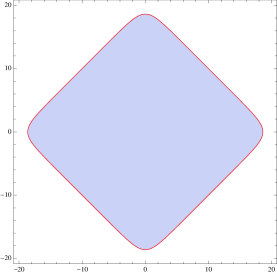
Figure 2: The region of phase space (3.1) for ABJM theory, at large energy.

A natural starting point to find the spectrum is to use the Bohr–Sommerfeld approximation, which in this generalized setting goes as follows. Let ${\rm{Vol}}_{\rm cl}(E,M)$ be the classical phase space volume, i.e. the volume of the region

$$\mathcal{R}_{\rm cl}(E)=\left\{\left(x,p\right)\in\mathbb{R}^{2}:\rho_{\rm cl}(x,p)\leq{\rm e}^{-E}\right\}.$$ (3.1)

Here we denoted by $\rho_{\rm cl}(x,p)$ the classical limit of the quantum operator $\hat{\rho}$, which is given by

$$\rho_{\rm cl}(x,p)={\rm e}^{-T(p)-U(x,M)},$$ (3.2)

where

$$T(p)=\log\left(2\cosh{p\over 2}\right),\quad U(x,M)=-\log\left(V_{M}(x)\right).$$ (3.3)

The Bohr–Sommerfeld quantization condition reads

$$\text{Vol}_{\rm cl}(E,k,M)=2\pi\hbar\left(n+{1\over 2}\right),\qquad n=0,1,2,\cdots$$ (3.4)

For large values of the energy one finds

$$\text{Vol}_{\rm cl}(E,k,M)\approx 8E^{2},$$ (3.5)

as shown for instance in Figure 2. Notice that the region $\mathcal{R}_{\rm cl}(E)$ has a finite volume, corresponding to the fact that the operator $\hat{\rho}$ has a discrete spectrum. In mp it was pointed out that the classical volume receives two types of quantum corrections, perturbative and non perturbative in $\hbar$, and there should be a fully “quantum” version of the classical function $\text{Vol}_{\rm cl}(E,k,M)$ incorporating these corrections, which we will denote by $\text{Vol}(E,k,M)$. It is convenient to write the quantum volume as in km ,

$$\text{Vol}(E,k,M)=\text{Vol}_{\rm{p}}(E,k,M)+\text{Vol}_{{\rm{np}}}(E,k,M),$$ (3.6)

where $\text{Vol}_{\rm{p}}(E,k,M)$ contains the full series of perturbative corrections in $\hbar$, while $\text{Vol}_{{\rm{np}}}(E,k,M)$ contains the non-perturbative corrections in $\hbar$. The Bohr–Sommerfeld quantization condition should be promoted to an exact WKB quantization condition of the form

$$\text{Vol}(E,k,M)=2\pi\hbar\left(n+{1\over 2}\right),\qquad n=0,1,2,\cdots$$ (3.7)

similar to what happens in some problems in ordinary Quantum Mechanics zj .

Our goal is to extract the exact quantum volume from our knowledge of the exact grand potential. A first attempt to do this was presented in km . Although the strategy of km leads to the correct result in the case of $k=1,2$, it involves many technical difficulties in the study of the non-perturbative sector. Here we overcome these difficulties by using the approach of cgm , where the quantum volume and the spectrum are computed by studying the zeros of the spectral determinant . Therefore, we will first find a convenient expression for the spectral determinant of these theories.

In the case of maximally supersymmetric theories, it was shown in cgm that the sum appearing in (2.26) can be written in terms of Jacobi theta functions. It is easy to see, by a computation similar to the one presented in ghm , that the spectral determinant for ABJ(M) theory (2.26) is given by

$$\Xi(\mu,k,M)={\rm e}^{J(\mu,k,M)}\Theta(\mu,k,M),$$ (3.8)

where

$$\Theta(\mu,k,M)=\sum_{n\in{\mathbb{Z}}}\exp\biggl{\{} -4\pi^{2}n^{2}C(k)\mu_{\rm eff}+2\pi{\rm i}n\left(C(k)\mu_{\rm eff}^{2}+B(k,M)+\widetilde{J}_{b}(\mu_{\rm eff},k,M)\right)$$ (3.9)

$$+J_{\rm WS}(\mu_{\rm eff}+2\pi{\rm i}n,k,M)-J_{\rm WS}(\mu_{\rm eff},k,M)-{8\pi^{3}{\rm i}n^{3}\over 3}C(k)\biggr{\}}.$$

We will call this function a generalized theta function.

As we noted in (2.19), the spectrum of energies in (2.14) can be obtained by looking at the zeros of the spectral determinant, by setting

$$\mu=E+\pi{\rm i}.$$ (3.10)

As it was found in cgm ; ghm , this involves looking at the zeros of the (generalized) theta function, and leads to a quantization condition of the form (3.7) which incorporates all the perturbative and non-perturbative corrections to the Bohr–Sommerfeld condition (3.4). It is easy to see that

$$\Theta(E+\pi{\rm i},k,M)={\rm e}^{\zeta}\sum_{n\in{\mathbb{Z}}}\exp\biggl{\{} -4\pi^{2}(n+1/2)^{2}C(k)E_{\rm eff}-{8\pi^{3}{\rm i}(n+1/2)^{3}\over 3}C(k)$$ (3.11)

$$+2\pi{\rm i}(n+1/2)\left(C(k)E_{\rm eff}^{2}+B(k,M)+\tilde{J}_{b}(E_{\rm eff}+\pi{\rm i},k,M)\right)$$

$$+f_{\rm WS}(E_{\rm eff}+\pi{\rm i},n)-{1\over 2}f_{\rm WS}(E_{\rm eff}+\pi{\rm i},-1)\ \biggr{\}}.$$

In this equation we have introduced, in analogy with (2.32), the “effective” energy

$$E_{\rm eff}=E-\frac{1}{2}\sum_{\ell=1}^{\infty}(-1)^{M\ell}\hat{a}_{\ell}(k){\rm e}^{-2\ell E}.$$ (3.12)

In addition, we have

$$f_{\rm WS}(\mu,n) =\sum_{m\geq 1}d_{m}(k,M)\left({\rm e}^{-8\pi{\rm i}mn/k}-1\right)(-1)^{m}{\rm e}^{-4m\mu/k},$$ (3.13)

so that

$$f_{\rm WS}(E_{\rm eff}+\pi{\rm i},-1)=2{\rm i}\sum_{m\geq 1}d_{m}(k,M)\sin{4\pi m\over k}(-1)^{m}{\rm e}^{-4mE_{\rm eff}/k}.$$ (3.14)

We also have that

$$\zeta ={2\over k}E_{\rm eff}-\pi{\rm i}\left({2\over\pi^{2}k}E_{\rm eff}^{2}+B(k,M)+\tilde{J}_{b}(E_{\rm eff}+\pi{\rm i},k,M)\right)$$ (3.15)

$$+{1\over 2}f_{\rm WS}(E_{\rm eff}+\pi{\rm i},-1)+{2\pi{\rm i}\over 3k}.$$

Note that, if we just take into account in the generalized theta function (3.11) the terms with $n=0,-1$, we obtain the quantization condition

$$\cos\left(\pi\Omega(E,k,M)\right)=0,$$ (3.16)

where

$$\Omega(E,k,M) =C(k)E_{\rm eff}^{2}+B(k,M)-{\pi^{2}C(k)\over 3}+\sum_{\ell=1}^{\infty}\widetilde{b}_{\ell}(k)(-1)^{M\ell}{\rm e}^{-2\ell E_{\rm eff}}$$ (3.17)

$$\quad-{1\over\pi}\sum_{m\geq 1}(-1)^{m}d_{m}(k,M)\sin\left({4\pi m\over k}\right){\rm e}^{-4mE_{\rm eff}/k}.$$

This is precisely the quantization condition proposed in km ; kallen . However, there will be in general corrections to this condition, due to the remaining terms in (3.11). In order to take them into account systematically, let us call this correction $\lambda(E)$ and write the exact quantization condition as

$$\Omega(E,k,M)+\lambda(E)=s+{1\over 2},\quad s=0,1,2,\dots.$$ (3.18)

A straightforward calculation shows that $\lambda(E)$, which is non-perturbative in $k$ (i.e. in $\hbar$), is determined by the following equation ghm

$$\sum_{n\geq 0}{\rm e}^{-\frac{8n(n+1)}{k}E_{\rm eff}}(-1)^{n}{\rm e}^{f_{\text{c}}(n)}\sin\left(\frac{8\pi n(n+1)(2n+1)}{3k}+f_{\text{s}}(n)+2\pi\left(n+\frac{1}{2}\right)\lambda(E)\right)=0,$$ (3.19)

where

$$f_{\text{c}}(n) =\sum_{m\geq 1}(-1)^{m}d_{m}(k,M)\biggl{[}\cos\left(\frac{4\pi m(2n+1)}{k}\right)-\cos\left(\frac{4\pi m}{k}\right)\biggr{]}{\rm e}^{-\frac{4m}{k}E_{\rm eff}},$$ (3.20)

$$f_{\text{s}}(n) =\sum_{m\geq 1}(-1)^{m}d_{m}(k,M)\biggl{[}\sin\left(\frac{4\pi m(2n+1)}{k}\right)-(2n+1)\sin\left(\frac{4\pi m}{k}\right)\biggr{]}{\rm e}^{-\frac{4m}{k}E_{\rm eff}}.$$

We also conclude from this analysis that the exact quantum volume is given by

$${\rm Vol}(E,k,M)=2\pi\hbar\left(\Omega(E,k,M)+\lambda(E)\right).$$ (3.21)

Note that the perturbative part of this quantum volume is given precisely by the all-orders WKB perturbative contribution, encoded in the quantum B-period,

$${1\over 2\pi\hbar}{\rm Vol}_{\rm p}(E,k,M)=C(k)E_{\rm eff}^{2}+B(k,M)-{\pi^{2}C(k)\over 3}+\sum_{\ell=1}^{\infty}\widetilde{b}_{\ell}(k)(-1)^{M\ell}{\rm e}^{-2\ell E_{\rm eff}},$$ (3.22)

while the non-perturbative contribution is given by

$${1\over 2\pi\hbar}{\rm Vol}_{\rm np}(E,k,M)=-{1\over\pi}\sum_{m\geq 1}(-1)^{m}d_{m}(k,M)\sin\left({4\pi m\over k}\right){\rm e}^{-4mE_{\rm eff}/k}+\lambda(E).$$ (3.23)

The perturbative and the non-perturbative part are separately divergent when $k$ is rational, as noted in km , but the total quantum volume (3.21) is smooth, since the singularities cancel as a consequence of the HMO mechanism (indeed, the quantum volume is obtained from the modified grand potential, which is singularity-free). The non-perturbative part is then needed to cancel the singularities in the WKB perturbative expansion, and it contains crucial information on the spectrum. For example, as shown in appendix A, when $k$ is an integer, the finite part of $\tilde{J}_{b}(E_{\rm eff}+\pi{\rm i},k,M)$ vanishes and the quantum volume is largely determined by the worldsheet instanton contribution.

The correction $\lambda(E)$ can be computed analytically, in a series expansion in ${\rm e}^{-4E_{\rm eff}/k}$. It is easy to see that $\lambda(E)$ is of the form

$$\lambda(E)=\sum_{\ell\geq 1}\lambda_{\ell}\,{\rm e}^{-\frac{4\ell+12}{k}E_{\rm eff}},$$ (3.24)

where the first few terms are explicitly given by

$$\lambda_{1} =\frac{1}{\pi}\sin(16x),$$ (3.25)

$$\lambda_{2} =\frac{4}{\pi}\sin^{2}(4x)\sin(20x)d_{1},$$

$$\lambda_{3} =\frac{8}{\pi}\sin^{2}(4x)\sin(24x)[\sin^{2}(4x)d_{1}^{2}-2\cos^{2}(4x)d_{2}],$$

$$\lambda_{4} =\frac{4}{3\pi}\sin^{2}(4x)\sin(28x)[3(d_{1}^{3}-2d_{1}d_{2}+3d_{3})-4\cos(8x)(d_{1}^{3}-3d_{3})$$

$$\quad+\cos(16x)(d_{1}^{3}+6d_{1}d_{2}+6d_{3})]$$

with

$$d_{1} =d_{1}(k,M)=-\cos\left(2Mx\right)\csc^{2}\left(2x\right),$$ (3.26)

$$d_{2} =d_{2}(k,M)=-\csc^{2}\left(2x\right)-\frac{1}{2}\cos\left(4Mx\right)\csc^{2}\left(4x\right),$$

$$d_{3} =d_{3}(k,M)=-3\cos\left(2Mx\right)\csc^{2}\left(2x\right)-\frac{1}{3}\cos\left(6Mx\right)\csc^{2}\left(6x\right),$$

and we have denoted

$$x={\pi\over k}.$$ (3.27)

Note that, when $k=1,2,4$, we have that $f_{\rm s}(n)=0$, and the first term in the argument of the sine in (3.19) is always a multiple of $\pi$. Therefore, the solution to (3.19) is $\lambda(E)=0$, i.e. the correction vanishes and the quantization condition of km ; kallen is exact.

	Energy levels for $k=3,M=0$
Order	$E_{0}$	$E_{1}$
${\rm e}^{-4E/3}$	${\underline{2.65}297702084083921}$	4.68940459079460092512108986442
${\rm e}^{-12E/3}$	${\underline{2.65156}164019289190}$	4.68940134450544960666103687122
${\rm e}^{-24E/3}$	${\underline{2.65156833}993530136}$	4.68940134457031678330042507336
${\rm e}^{-32E/3}$	${\underline{2.65156833716}940289}$	4.68940134457031677561757482976
${\rm e}^{-40E/3}$	${\underline{2.651568337168}75544}$	4.68940134457031677561753154101
${\rm e}^{-52E/3}$	${\underline{2.651568337168857}61}$	4.68940134457031677561753154681
Numerical value	2.65156833716885755	4.68940134457031677561753154681

Table 1: The first two energy levels for $k=3$ and $M=0$ calculated analytically from (3.18). In the last line numerical values evaluated by the method in appendix C are given. At each order of the approximation, we underline the digits which agree with the numerical result.

	Energy levels for $k=5,M=0$
Order	$E_{0}$	$E_{1}$
${\rm e}^{-4E/5}$	${\underline{3.0}475013693}$	5.79353763401508120749977
${\rm e}^{-16E/5}$	${\underline{3.0724}584475}$	5.79369469126135544218070
${\rm e}^{-32E/5}$	${\underline{3.072435}9155}$	5.79369469107338173784939
${\rm e}^{-48E/5}$	${\underline{3.07243583}57}$	5.79369469107338158412549
Numerical value	3.0724358360	5.79369469107338158412559

	Energy levels for $k=6,M=0$
Order	$E_{0}$	$E_{1}$
${\rm e}^{-4E/6}$	${\underline{3.2}1322311}$	6.23111654150891713732
${\rm e}^{-16E/6}$	${\underline{3.23}510192}$	6.23141999560231213049
${\rm e}^{-32E/6}$	${\underline{3.23464}705}$	6.23141998018954896785
${\rm e}^{-48E/6}$	${\underline{3.234644}06}$	6.23141998018953286312
Numerical value	3.23464413	6.23141998018953286330

Table 2: The first two energy levels for $k=5,6$ and $M=0$ calculated analytically from (3.18).

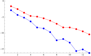
Figure 3: The difference $\Delta_{0}^{(k)}(m)$ (3.30) as a function of $m$, the number of instantons included in the computation. The line on the bottom (in blue) gives $\Delta_{0}^{(3)}(m)$, while the line on the top (in red) gives $\Delta_{0}^{(5)}(m)$.

	Energy levels for $k=3,M=1$
Order	$E_{0}$	$E_{1}$
${\rm e}^{-8E/3}$	${\underline{3.48669}71392036144}$	5.190229102060787166657584
${\rm e}^{-12E/3}$	${\underline{3.4866953}311076197}$	5.190229100088979204304574
${\rm e}^{-20E/3}$	${\underline{3.4866953293248}867}$	5.190229100088834784550474
${\rm e}^{-28E/3}$	${\underline{3.48669532933487}93}$	5.190229100088834796616934
Numerical value	3.4866953293348782	5.190229100088834796616924

Table 3: The first two energy levels for $k=3,M=1$ calculated analytically from (3.18).

	Energy levels for $k=5,M=2$
Order	$E_{0}$	$E_{1}$
${\rm e}^{-8E/3}$	${\underline{4.8544}694530582}$	6.95012371466050570772
${\rm e}^{-12E/3}$	${\underline{4.854453}3648860}$	6.95012364154401512072
${\rm e}^{-20E/3}$	${\underline{4.854453651}9209}$	6.95012364179272664768
${\rm e}^{-28E/3}$	${\underline{4.85445365153}25}$	6.95012364179271448721
Numerical value	4.8544536515315	6.95012364179271448613

Table 4: The first two energy levels for $k=5,M=2$ calculated analytically from (3.18).

Let us now give some concrete results for the correction series (3.24). In the case of ABJM theory, with $M=0$, the first few corrections read

$$\lambda_{1} =\frac{1}{\pi}\sin\left(16x\right),$$ (3.28)

$$\lambda_{2} =-\frac{4}{\pi}\sin^{2}(4x)\sin(20x)\csc^{2}(2x),$$

$$\lambda_{3} =\frac{8}{\pi}\sin(24x)\csc^{2}(2x)\left(3\sin^{2}(4x)\sin^{2}(6x)+\sin^{2}(2x)\sin^{2}(8x)+\sin^{2}(10x)\right),$$

$$\lambda_{4} =-\frac{8}{\pi}\sin^{2}(4x)\sin(28x)\csc^{2}(2x)\bigl{(}23+22\cos(4x)+19\cos(8x)+4\cos(12x)+3\cos(16x)\bigr{)}.~{}~{}$$

The results for $\lambda_{1},\lambda_{2}$ and $\lambda_{3}$ are in perfect agreement with the results of huang based on numerical fitting. We can check as well the higher order corrections by performing a detailed numerical analysis. First of all, we compute the first two energy levels in (2.14), with high precision. To do this, we follow a procedure inspired by the analysis of hmo and summarized in Appendix C. On the other hand, we use (3.19) to compute the corrections to the quantum volume up to

$$\lambda_{10}{\rm e}^{-{52\over k}E_{\rm eff}}.$$ (3.29)

The results are shown in tables 1 and 2, for $k=3,5,6$. As expected, the more instanton corrections we include in the analytic computation, the better we approach the numerical value. This can be seen in detail by considering the quantity

$$\Delta_{0}^{(k)}(m)=\log_{10}\left|E^{\rm num}_{0}(k)-E^{(m)}_{0}(k)\right|,$$ (3.30)

where $E^{\rm num}_{0}$ is the numerical value of the ground state energy, and $E^{(m)}_{0}$ is the value computed from (3.19) by including the first $m$ instanton corrections. As shown in Fig. 3, $E^{(m)}_{0}$ converges to $E^{\rm num}_{0}$ as $m$ grows. However, it does not converge monotonically, in contrast to what happened in the numerical analysis of km for $k=1,2$ and $M=0$. In tables 3, 4 we give additional numerical evidence for the validity of the quantization condition in the ABJ case with $M\neq 0$.

4 A case study with $\mathcal{N}=6$ supersymmetry

As emphasized in ghm , the quantization condition studied in the previous section is a consequence of a stronger result, namely our explicit formula (3.8) for the spectral determinant. In principle, using this formula, one can compute the canonical partition functions by performing an expansion around $\kappa=0$ as in (2.21). In cgm this was checked in detail in the maximally supersymmetric cases, by using the computations of the partition functions in py ; hmo ; hmo2 ; honda-o ; abj-moriyama . In the case with maximal supersymmetry, the generalized theta function becomes a standard Jacobi theta function, and the higher genus contribution to the modified grand potential vanish, so the analysis of the spectral determinant is relatively straightforward.

In this section we analyze in detail a case with ${\cal N}=6$ supersymmetry, namely ABJM theory with $k=4$. This case is slightly richer than the maximally supersymmetric cases because the grand potential involves the all genus worldsheet instantons. However, the generalized theta function of this theory becomes a conventional theta function, as in the maximally supersymmetric cases. Therefore this case is not the most generic one, but it is a good starting point to start exploring the spectral determinants of theories with ${\cal N}=6$ supersymmetry.

It follows from (2.27) that the grand potential of ABJM theory with $k=4$ is given by

$$J(\mu,4)=J^{({\rm p})}(\mu_{\rm eff},4)+J^{\rm WS}(\mu_{\rm eff},4)+\mu_{\rm eff}\widetilde{J}_{b}(\mu_{\rm eff},4)+\widetilde{J}_{c}(\mu_{\rm eff},4).$$ (4.1)

To calculate this quantity we have to take the limit $k\rightarrow 4$ in the general expression and be careful with the poles, as in cgm . These however cancel, as we recalled above, so we can compute (4.1) by considering only its finite part. In particular $\widetilde{J}_{b}(\mu_{\rm eff},4)$ has no finite part, as shown in appendix A, while the finite part of $\widetilde{J}_{c}(\mu_{\rm eff},4)$ is

$${1\over 12}\left(-\log\left(1-16y^{2}\right)+\tilde{\varpi}_{1}(-y^{2})\right),\quad y={\rm e}^{-\mu},$$ (4.2)

where

$$\tilde{\varpi}_{1}(z)=-4z\,_{4}F_{3}\left(1,1,\frac{3}{2},\frac{3}{2};2,2,2;-16z\right).$$ (4.3)

Let us now look at the worldsheet instanton part. For general $k$ and $M=0$ the expression (2.39) reads

$$J^{\rm WS}(\mu,k)=\sum_{g\geq 0}\sum_{w,d\geq 1}{1\over w}(-1)^{dw}n_{g}^{d}\left(2\sin{2\pi w\over k}\right)^{2g-2}{\rm e}^{-4dw\mu/k}.$$ (4.4)

It is convenient to split the sum over $w$ into even and odd part. This leads to

$$J^{\rm WS}(\mu,k) =\sum_{g\geq 0}\sum_{w,d\geq 1}{1\over 2w}n_{g}^{d}\left(2\sin{2\pi w\over(k/2)}\right)^{2g-2}{\rm e}^{-4dw\mu/(k/2)}$$ (4.5)

$$\quad+\sum_{g\geq 0}\sum_{w,d\geq 1}{1\over 2w-1}(-1)^{d}n_{g}^{d}\left(2\sin{2\pi(2w-1)\over k}\right)^{2g-2}{\rm e}^{-4d(2w-1)\mu/k}.$$

When $k=4$, the first part is (up to a factor $1/2$) precisely the worldsheet instanton part of the modified grand potential for the maximally supersymmetric theory $(k,M)=(2,1)$ analyzed in cgm . The second part is a non trivial quantity which contains all genus contributions. We can then write the worldsheet instanton part of (4.1) as

$$J^{\rm WS}(\mu_{\rm eff},4)={1\over 2}J^{\rm WS}(\mu_{\rm eff},2,1)+I(\mu_{\rm eff}).$$ (4.6)

The first term was computed in cgm and reads

$$J^{\rm WS}(\mu,2,1)={\mu_{\rm eff}^{2}\over 2\pi^{2}}\partial^{2}_{t}F^{\rm inst}_{0}(t)-{\mu_{\rm eff}\over 2\pi^{2}}\partial_{t}F^{\rm inst}_{0}(t)+{1\over 4\pi^{2}}F^{\rm inst}_{0}(t)+F_{1}^{\rm inst}(t).$$ (4.7)

Here we used $t=2\mu_{\rm eff}$ and

$$F^{\rm inst}_{0}(t)=\sum_{d,w}n_{0}^{d}{1\over w^{3}}{\rm e}^{-dwt},\quad F^{\rm inst}_{1}(t)=\sum_{d,w}\left({n_{0}^{d}\over 12}+n_{1}^{0}\right){\rm e}^{-dwt}.$$ (4.8)

The second part of $J^{\rm WS}$ contains contributions at all genera and can be written as

$$I(\mu_{\rm eff})=\sum_{g\geq 0}\sum_{w,d\geq 1}{(-1)^{d}n_{g}^{d}\over 2w-1}4^{g-1}{\rm e}^{-d(2w-1)\mu_{\rm eff}}=\sum_{g\geq 0}\sum_{d\geq 1}4^{g-1}(-1)^{d}n^{d}_{g}\tanh^{-1}\left({\rm e}^{-d\mu_{\rm eff}}\right).$$ (4.9)

By looking at the small $y$ expansion of this quantity we conjecture that it can be resummed in closed form in terms of an elliptic integral of the first kind,

$$I(\mu_{\rm eff})=-\frac{1}{4}\log\left(\frac{2K\left(16y^{2}\right)}{\pi}\right)+{1\over 4}\tanh^{-1}\left(4y\right).$$ (4.10)

We have checked the above equality order by order in a series expansion at small $y$, but we do not have a general proof of it. However, we will see that this conjecture reproduces the correct $Z(N,4)$ appearing in the large $y$ expansion of the spectral determinant (2.25). This strongly suggests that (4.10) is a true identity. The existence of an identity like this is remarkable, since it resums the all-genus Gopakumar–Vafa expansion of the free energy. This resummation is needed if we want to reproduce the canonical partition functions: this requires an expansion around $y\rightarrow\infty$, while the original Gopakumar–Vafa expansion only holds at large radius, i.e. for $y\rightarrow 0$.

By using (4.10) one finds

$$J(\mu,4) =A(4,0)+F_{1}(t)+F_{1}^{\rm NS}(t)+{\mu\over 4}+\frac{1}{4}\tanh^{-1}\left(4{\rm e}^{-\mu}\right)$$ (4.11)

$$\quad+{1\over 8\pi^{2}}\left(F_{0}(t)-t\partial_{t}F_{0}(t)+{1\over 2}t^{2}\partial_{t}^{2}F_{0}(t)\right),$$

where

$$F_{0}(t) ={t^{3}\over 6}+F_{0}^{\rm inst}(t),$$ (4.12)

$$F_{1}(t) =-{1\over 12}\log\left[64y^{2}(1-16y^{2})\right]-{1\over 2}\log\left({K(16y^{2})\over\pi}\right),$$

$$F_{1}^{\rm NS}(t) =-{1\over 24}\log{(1-16y^{2})\over y^{4}}.$$

The constant $A(4,0)$ is the standard constant map contribution of ABJM, whose exact value is given by

$$A(4,0)=-\frac{\zeta(3)}{4\pi^{2}}-\frac{\log(2)}{2}.$$ (4.13)

The derivative of the grand potential takes the following closed form,

$$\partial_{\mu}J(\mu,k=4)=\frac{\mu_{\rm eff}^{2}}{8\left(1-16y^{2}\right)K\left(16y^{2}\right)^{2}}-\frac{E\left(16y^{2}\right)}{2\left(16y^{2}-1\right)K\left(16y^{2}\right)}+\frac{1-2y}{8y-2}+{1\over 4}.$$ (4.14)

The large $\mu$ expansion of (4.11) reads

$$J(\mu,4) =\frac{\mu^{3}}{6\pi^{2}}+\frac{\mu}{4}-\frac{\zeta(3)}{4\pi^{2}}-\frac{\log(2)}{2}+y+\frac{\left(-4\mu^{2}-2\mu-1\right)y^{2}}{2\pi^{2}}$$ (4.15)

$$\quad+\frac{16y^{3}}{3}+\frac{\left(-208\mu^{2}-4\mu+32\pi^{2}-9\right)y^{4}}{16\pi^{2}}+\frac{256y^{5}}{5}+\mathcal{O}(y^{6}).$$

Once we know the modified grand potential, we can use (2.22) and (2.26) to obtain the grand canonical partition function or spectral determinant:

$$\Xi(\kappa,4)={\rm e}^{J(\mu,4)}\vartheta_{3}\left({1\over 2}\left(\xi-{\tau\over 4}-{1\over 12}\right),{\tau\over 2}\right),$$ (4.16)

where

$$\tau={2{\rm i}\over\pi}\partial_{t}^{2}F_{0}(t),\quad\xi={1\over 2\pi}\left(t\partial_{t}^{2}F_{0}(t)-\partial_{t}F_{0}(t)\right).$$ (4.17)

Note that, although this theory is not maximally supersymmetric, the generalized theta function becomes in this case a Jacobi theta function. As explained in cgm ; ghm the spectrum is determined by the zeros of the theta function, and we find the exact quantization condition

$${\xi}-{\tau\over 4}-{1\over 12}=2n+1,\quad n=0,1,2,\cdots$$ (4.18)

Interestingly, the quantum volume for $k=4$ is exactly related to that for $k=2$ and $M=1$

$$\text{Vol}(E,k=4)={1\over 2}\left({\xi}-{\tau\over 4}-{1\over 12}\right){16\pi^{2}}=\text{Vol}(E,k=2,M=1)+4\pi^{2},$$ (4.19)

where $\text{Vol}(E,k=2,M=1)$ is the quantum volume for the maximally supersymmetric theory with $k=2$, $M=1$ obtained in cgm . Notice that, as we mentioned before, in this case the approximate quantization condition of km is exact and does not need additional corrections.

By following the arguments of cgm , we can now use modular properties and analytic continuation to write the special determinant (4.16) in the orbifold frame, i.e. in the region $\mu\rightarrow-\infty$, where we make contact with the expansion (2.21). This will allow us to compute the exact values of $Z(N,4)$ for finite $N$, which provides a check of the formula (3.8). In order to proceed we introduce the orbifold periods dmp :

$$\lambda ={\rm i}{\kappa\over 8\pi}{~{}}_{3}F_{2}\left(\frac{1}{2},\frac{1}{2},\frac{1}{2};1,\frac{3}{2};\frac{\kappa^{2}}{16}\right),$$ (4.20)

$$\partial_{\lambda}{\cal F}_{0}(\lambda) ={\rm i}{\kappa\over 4}G^{2,3}_{3,3}\left(\begin{array}[]{ccc}{1\over 2},&{1\over 2},&{1\over 2}\\ 0,&0,&-{1\over 2}\end{array}\biggl{|}{\kappa^{2}\over 16}\right)-{\pi^{2}\kappa\over 2}{~{}}_{3}F_{2}\left(\frac{1}{2},\frac{1}{2},\frac{1}{2};1,\frac{3}{2};\frac{\kappa^{2}}{16}\right).$$

Here, ${\cal F}_{0}(\lambda)$ is the genus zero free energy in the orbifold frame, normalized in such a way that is expansion around $\lambda=0$ is given by

$${\cal F}_{0}(\lambda)=-4\pi^{2}\lambda^{2}\left(\log(2\pi\lambda)-\frac{3}{2}-\log(4)\right)+\cdots$$ (4.21)

Using modular properties of the periods and analytic continuation we find

$$\Xi(\kappa,4) =\exp\biggl{[}\frac{1}{4}\tanh^{-1}\left(\frac{{\rm e}^{\mu}}{4}\right)+{\mu\over 4}-{1\over 2\pi^{2}}\left({\cal F}_{0}(\lambda)-\lambda\partial_{\lambda}{\cal F}_{0}(\lambda)+{1\over 2}\lambda^{2}\partial^{2}_{\lambda}{\cal F}_{0}(\lambda)\right)\biggr{]}$$ (4.22)

$$\times\exp\biggl{[}{\cal F}_{1}+F_{1}^{\rm NS}-{{\rm i}\pi\over 8}+\biggl{]}\vartheta_{3}\left(\bar{\xi}-{1\over 4},2{\bar{\tau}}\right),$$

where

$$\bar{\tau}=-{1\over 8\pi^{3}{\rm i}}\partial_{\lambda}^{2}{\cal F}_{0}(\lambda),\qquad\bar{\xi}={{\rm i}\over 4\pi^{3}}\left(\lambda\partial_{\lambda}^{2}{\cal F}_{0}(\lambda)-\partial_{\lambda}{\cal F}_{0}(\lambda)\right).$$ (4.23)

The genus one free energy in the orbifold frame is given by

$${\cal F}_{1}=-\log\eta\left(2\bar{\tau}\right)-{1\over 2}\log 2.$$ (4.24)

The small $\kappa$ expansion of (4.16) is now straightforward and one finds

$${\cal F}_{1}+F_{1}^{\rm NS}(t)-{{\rm i}\pi\over 8}+\frac{1}{4}\tanh^{-1}\left(\frac{{\rm e}^{\mu}}{4}\right)+{\mu\over 4} =\frac{\kappa}{16}+\frac{\kappa^{3}}{768}+\frac{\kappa^{4}}{32768}+\mathcal{O}(\kappa^{5}),$$ (4.25)

$$-{1\over 2\pi^{2}}\left({\cal F}_{0}(\lambda)-\lambda\partial_{\lambda}{\cal F}_{0}(\lambda)+{1\over 2}\lambda^{2}\partial^{2}_{\lambda}{\cal F}_{0}(\lambda)\right) =-\frac{\kappa^{2}}{64\pi^{2}}-\frac{\kappa^{4}}{3072\pi^{2}}+\mathcal{O}(\kappa^{5}),$$

$$\vartheta_{3}\left(\bar{\xi}-{1\over 4},2{\bar{\tau}}\right) =1-\frac{\kappa^{3}}{256\pi}+\mathcal{O}(\kappa^{5}).$$

Hence we have

$$\Xi(\kappa,4)=1+{\kappa\over 16}+\frac{\pi^{2}-8}{512\pi^{2}}\kappa^{2}+\mathcal{O}(\kappa^{3}),$$ (4.26)

which reproduces the computation of the very first $Z(N,4)$ in hmo2 . Of course we can push the computation at higher order in $\kappa$ and reproduce all known $Z(N,4)$ for higher $N$.

5 Factorization of the spectral determinant

Since the potential $V_{M}(x)$ appearing in the ABJ(M) spectral problem is even, the eigenfunctions $\phi_{n}(x)$ (2.14) can be classified according to their parity, as in ordinary one-dimensional quantum-mechanical problems. The even energy levels correspond to even eigenfunctions, while the odd energy levels correspond to odd eigenfunctions. Therefore, we can split the spectral determinant (2.16) according to the parity of the eigenfunctions, and we define

$$\Xi_{+}(\kappa,k,M)=\prod_{n=0}^{\infty}(1+\kappa{\rm e}^{-E_{2n}}),\qquad\Xi_{-}(\kappa,k,M)=\prod_{n=0}^{\infty}(1+\kappa{\rm e}^{-E_{2n+1}}).$$ (5.1)

If we introduce the operators with even/odd parity

$$\rho_{\pm}(x_{1},x_{2})=\frac{\rho(x_{1},x_{2})\pm\rho(x_{1},-x_{2})}{2},$$ (5.2)

the spectral determinants can be also written as

$$\Xi_{\pm}(\kappa,k,M)=\det(1+\kappa\hat{\rho}_{\pm})=\exp\left[-\sum_{n=1}^{\infty}\frac{(-\kappa)^{n}}{n}\mathop{\rm Tr}\nolimits\hat{\rho}_{\pm}^{n}\right].$$ (5.3)

Notice that by construction, one immediately gets

$$\Xi(\kappa,k,M)=\Xi_{+}(\kappa,k,M)\Xi_{-}(\kappa,k,M).$$ (5.4)

In this section we present an exact expression for the spectral determinants (5.1) in the case of $k=1,M=0$. We do not have a first principles derivation of such expressions, so we postulate a form that can be subsequently verified in detail. The expressions we propose are the following,

$$\Xi_{+}(\kappa,1) =e^{J_{+}(\mu,1)}\vartheta_{3}\left(\frac{1}{2}\left(\frac{\xi}{2}+\frac{5}{24}\right),\frac{\tau}{2}\right),$$ (5.5)

$$\Xi_{-}(\kappa,1) =e^{J_{-}(\mu,1)}\vartheta_{4}\left(\frac{1}{2}\left(\frac{\xi}{2}+\frac{5}{24}\right),\frac{\tau}{2}\right).$$

In these expressions,

$$J_{+}(\mu,1) =\frac{f_{0}(\mu)}{2}+f_{1}(\mu)+\frac{7}{16}\mu+A_{+}(1)+\frac{1}{8}\log\left(\frac{1+2\sqrt{2}e^{-\mu}+4e^{-2\mu}}{1-2\sqrt{2}e^{-\mu}+4e^{-2\mu}}\right),$$ (5.6)

$$J_{-}(\mu,1) =\frac{f_{0}(\mu)}{2}+f_{1}(\mu)-\frac{1}{16}\mu+A_{-}(1)-\frac{1}{8}\log\left(\frac{1+2\sqrt{2}e^{-\mu}+4e^{-2\mu}}{1-2\sqrt{2}e^{-\mu}+4e^{-2\mu}}\right),$$

where

$$f_{0}(\mu) =\frac{1}{16\pi^{2}}\left(F_{0}(t)-t\partial_{t}F_{0}(t)+\frac{t^{2}}{2}\partial_{t}^{2}F_{0}(t)\right),$$ (5.7)

$$f_{1}(\mu) =F_{1}(t)+F_{1}^{\rm NS}(t)$$

and

$$A_{+}(1)=-\frac{\zeta(3)}{16\pi^{2}}-\frac{3}{8}\log 2,\qquad A_{-}(1)=-\frac{\zeta(3)}{16\pi^{2}}+\frac{5}{8}\log 2,$$ (5.8)

In the $k=1$ context we should use $t=4\mu_{\rm eff}$ and

$$F_{0}(t)={t^{3}\over 6}+\sum_{d,w}n_{0}^{d}{(-1)^{dw}\over w^{3}}{\rm e}^{-dwt}.$$ (5.9)

The standard and refined genus one free energies are given in terms of $z={\rm e}^{-4\mu}$ as

$$F_{1}(t)= -{1\over 12}\log\left[64z(1+16z)\right]-{1\over 2}\log\left({K(-16z)\over\pi}\right),$$ (5.10)

$$F^{\rm NS}_{1}(t)= {1\over 12}\log z-{1\over 24}\log(1+16z).$$

As a first check of the proposal (5.5), let us show that the above expressions lead to the right quantization conditions, i.e. $\Xi_{\pm}(\kappa,1)$ vanish when $\mu=E_{2n}+{\rm i}\pi$, $\mu=E_{2n+1}+{\rm i}\pi$, respectively. Let us first recall the quantization condition for $k=1$ cgm

$${\xi\over 2}-{1\over 24}=m+{3\over 4},\quad m\geq 0.$$ (5.11)

It is easy to see that the zeros of $\Xi_{\pm}(E+{\rm i}\pi,1)$ are given by

$${\xi\over 2}-{1\over 24}= 2m+{3\over 4},\quad m\geq 0,$$ (5.12)

$${\xi\over 2}-{1\over 24}= 2(m+1)+{3\over 4},\quad m\geq 0,$$

which leads precisely to the odd and even energy levels for $k=1$ determined by (5.11).

As a second check, one can verify that

$$\Xi(\kappa,k)=\Xi_{+}(\kappa,k)\Xi_{-}(\kappa,k).$$ (5.13)

It is important to notice that the total grand potential $J(\mu,1)$ differs from the sum

$$J_{+}(\mu,1)+J_{-}(\mu,1)$$ (5.14)

by a term involving the genus one free energy. More precisely one has

$$J(\mu,1)=J_{+}(\mu,1)+J_{-}(\mu,1)-F_{1}(t)-F_{1}^{\rm NS}(t).$$ (5.15)

This additional contribution comes from the product of the two theta functions in $\Xi_{\pm}(\kappa,1)$.

The third test concerns the large $\mu$ expansion for $J_{\pm}(\mu,1)$. If we write

$$J_{+}(\mu,1) =\frac{\mu^{3}}{3\pi^{2}}+\frac{7}{16}\mu+A_{+}(1)+J_{+}^{\text{np}}(\mu,1),$$ (5.16)

$$J_{-}(\mu,1) =\frac{\mu^{3}}{3\pi^{2}}-\frac{1}{16}\mu+A_{-}(1)+J_{-}^{\text{np}}(\mu,1),$$

we find from the above expressions,

$$J_{+}^{\text{np}}(\mu,1) =\frac{1}{\sqrt{2}}{\rm e}^{-\mu}-\frac{4}{3\sqrt{2}}{\rm e}^{-3\mu}+\frac{16\mu^{2}+4\mu+1}{8\pi^{2}}{\rm e}^{-4\mu}-\frac{16}{5\sqrt{2}}{\rm e}^{-5\mu}+\frac{64}{7\sqrt{2}}{\rm e}^{-7\mu}$$ (5.17)

$$\quad+\biggl{[}-\frac{52\mu^{2}+\mu/2+9/16}{4\pi^{2}}+2\biggr{]}{\rm e}^{-8\mu}+\frac{256}{9\sqrt{2}}{\rm e}^{-9\mu}+\mathcal{O}({\rm e}^{-11\mu}),$$

$$J_{-}^{\text{np}}(\mu,1) =-\frac{1}{\sqrt{2}}{\rm e}^{-\mu}+\frac{4}{3\sqrt{2}}{\rm e}^{-3\mu}+\frac{16\mu^{2}+4\mu+1}{8\pi^{2}}{\rm e}^{-4\mu}+\frac{16}{5\sqrt{2}}{\rm e}^{-5\mu}-\frac{64}{7\sqrt{2}}{\rm e}^{-7\mu}$$

$$\quad+\biggl{[}-\frac{52\mu^{2}+\mu/2+9/16}{4\pi^{2}}+2\biggr{]}{\rm e}^{-8\mu}-\frac{256}{9\sqrt{2}}{\rm e}^{-9\mu}+\mathcal{O}({\rm e}^{-11\mu}).$$

These expansions can be reproduced from the expressions for the spectral traces of $\rho_{\pm}$, which were found in hmo up to $n=8$. The very first few values are given by

$$\begin{aligned} \mathop{\rm Tr}\nolimits\rho_{+}&=\frac{1}{4\sqrt{2}},\\ \mathop{\rm Tr}\nolimits\rho_{+}^{2}&=\frac{1}{16\pi},\\ \mathop{\rm Tr}\nolimits\rho_{+}^{3}&=\frac{3-2\sqrt{2}}{64},\\ \mathop{\rm Tr}\nolimits\rho_{+}^{4}&=\frac{1}{512}\left(1-\frac{8}{\pi^{2}}\right),\end{aligned}\qquad\quad\begin{aligned} \mathop{\rm Tr}\nolimits\rho_{-}&=\frac{1}{4}-\frac{1}{4\sqrt{2}},\\ \mathop{\rm Tr}\nolimits\rho_{-}^{2}&=\frac{-3+\pi}{16\pi},\\ \mathop{\rm Tr}\nolimits\rho_{-}^{3}&=\frac{-12+\pi+2\sqrt{2}\pi}{64\pi},\\ \mathop{\rm Tr}\nolimits\rho_{-}^{4}&=-\frac{8+32\pi-11\pi^{2}}{512\pi^{2}}.\end{aligned}$$ (5.18)

In fact, we can relate our factorized spectral determinants $\Xi_{\pm}$ to these spectral traces directly, by expressing them in terms of orbifold quantities, like in cgm . As shown in appendix B in detail, one finds the following small $\kappa$ expansion:

$$\log\Xi_{\pm}(\kappa,1)=-\sum_{n=1}^{\infty}\frac{(-\kappa)^{n}}{n}\mathop{\rm Tr}\nolimits\rho_{\pm}^{n},$$ (5.19)

which reproduces the exact values of $\mathop{\rm Tr}\nolimits\rho_{\pm}^{n}$. We have indeed computed $\mathop{\rm Tr}\nolimits\rho_{\pm}^{n}$ up to $n=44$ and compared them with the ones obtained from the orbifold expansion. The results show a perfect agreement.

6 Exact functional equations

In the previous section, we have considered the factorization of the spectral determinant. The reason why we focus on such a factorization is because the factorized spectral determinants $\Xi_{\pm}(\kappa,k,M)$ have a very rich structure. In particular, these functions satisfy a set of exact functional equations as we will see in this section. A similar property has already been found in the context of the spectral problem of certain ordinary differential equations (see voros ; dt ; blz5 for example), where it indicates an unexpected connection to integrable models. Our result extends this type of properties to the spectral problem of the Fredholm integral equation (2.14). We hope that our findings may give a clue of a connection to some integrable systems.

6.1 Wronskian-like relations

We consider the spectral determinant (2.16) and the factorized ones (5.1). Remarkably, these functions satisfy the following beautiful equations for given $k$ and $M$:

$${\rm e}^{\frac{M}{2k}\pi{\rm i}}\Xi_{+}\left({\rm i}\kappa,k,M+1\right)\Xi_{-}\left(-{\rm i}\kappa,k,M-1\right)$$ (6.1)

$$\quad-{\rm e}^{-\frac{M}{2k}\pi{\rm i}}\Xi_{+}\left(-{\rm i}\kappa,k,M+1\right)\Xi_{-}\left({\rm i}\kappa,k,M-1\right)=2{\rm i}\sin\left(\frac{M\pi}{2k}\right)\Xi\left(\kappa,k,M\right),$$

and

$${\rm e}^{-\frac{M}{2k}\pi{\rm i}}\Xi_{+}\left({\rm i}\kappa,k,M-1\right)\Xi_{-}\left(-{\rm i}\kappa,k,M+1\right)$$ (6.2)

$$\quad+{\rm e}^{\frac{M}{2k}\pi{\rm i}}\Xi_{+}\left(-{\rm i}\kappa,k,M-1\right)\Xi_{-}\left({\rm i}\kappa,k,M+1\right)=2\cos\left(\frac{M\pi}{2k}\right)\Xi\left(\kappa,k,M\right).$$

The equation (6.1) is quite similar to the so-called quantum Wronskian relation blz2 . We do not have a general proof for these relations but we can test them by computing the spectrum and its spectral traces from the quantization condition (3.18), and by doing small $\kappa$ expansions of the spectral determinants. This can be done for various values of the coupling $k$. Such tests strongly suggest that the functional equations (6.1) and (6.2) are widely valid not only for integral values of $k$, but also for non-integral values.

In particular, if $k$ is an integer, the equations (6.1) and (6.2) are essentially equivalent due to the Seiberg-like duality of ABJ theories abj . This duality relates the partition function for $(k,M)$ to the one for $(k,k-M)$. In terms of the spectral determinants, it simply says that

$$\Xi(\kappa,k,M)=\Xi(\kappa,k,k-M),\qquad\Xi_{\pm}(\kappa,k,M)=\Xi_{\pm}(\kappa,k,k-M).$$ (6.3)

If one considers the case $M=k-m$ in (6.2), one gets

$$-{\rm i}{\rm e}^{\frac{m}{2k}\pi{\rm i}}\Xi_{+}\left({\rm i}\kappa,k,k-m-1\right)\Xi_{-}\left(-{\rm i}\kappa,k,k-m+1\right)$$ (6.4)

$$\quad+{\rm i}{\rm e}^{-\frac{m}{2k}\pi{\rm i}}\Xi_{+}\left(-{\rm i}\kappa,k,k-m-1\right)\Xi_{-}\left({\rm i}\kappa,k,k-m+1\right)=2\sin\left(\frac{m\pi}{2k}\right)\Xi\left(\kappa,k,k-m\right).$$

Using the Seiberg-like duality $\Xi_{\pm}(\kappa,k,k-m\pm 1)=\Xi_{\pm}(\kappa,k,m\mp 1)$, it is easy to see that this equation is equivalent to (6.1) for $M=m$. We note that for non-integral $k$, the equations (6.1) and (6.2) are independent.

Moreover we conjecture another functional equation, which associates $\Xi_{\pm}(\kappa,k,1)$ to $\Xi(\kappa,k)$.

$$\Xi_{+}({\rm i}\kappa,k,1)\Xi_{+}(-{\rm i}\kappa,k,1)+\frac{\kappa}{4k}\Xi_{-}({\rm i}\kappa,k,1)\Xi_{-}(-{\rm i}\kappa,k,1)=\Xi(\kappa,k),\quad\forall k.$$ (6.5)

As before the identity (6.5) can be checked by computing the spectrum and by doing a small $\kappa$ expansion. We tested this relation for various values of the coupling $k$, and conjecture that it is valid for any $k$.

Let us comment on a consequence of these functional equations. For odd $k$, there are $k+1$ independent functions $\Xi_{\pm}(\kappa,k,M)$, ($M=0,\dots,\frac{k-1}{2}$) due to the Seiberg-like duality. A simple counting shows that the functional equation (6.1) (or equivalently (6.2)) gives $k-1$ independent constraints. This means that if we know the two functions $\Xi_{\pm}(\kappa,k)$ in the ABJM theory, all the other functions $\Xi_{\pm}(\kappa,k,M)$ in ABJ theory are determined by the functional equations. Similarly, for even $k$, the functional equation (6.1) gives $k-1$ independent constraints among the $k+2$ independent functions $\Xi_{\pm}(\kappa,k,M)$ ($M=0,\dots,\frac{k}{2}$). In this case, the equation (6.1) only does not determine the ABJ spectral determinants from the ABJM ones. Since we have the additional relation (6.5), one might expect that combining these equations, the ABJ spectral determinants are fixed, as for odd $k$. However, this is not the case. One can check that the equations (6.1) and (6.5) are not sufficient to determine all the ABJ spectral determinants only from the ABJM ones. We need more information for even $k$.

In the rest of this subsection we exploit our exact solution (5.5) to further test (6.5) in the case of $k=1$. More precisely, we are interested in studying the following identity:

$$\Xi_{+}({\rm i}\kappa,1)\Xi_{+}(-{\rm i}\kappa,1)+\frac{\kappa}{4}\Xi_{-}({\rm i}\kappa,1)\Xi_{-}(-{\rm i}\kappa,1)=\Xi(\kappa,1).$$ (6.6)

Notice that under $\kappa\to\pm{\rm i}\kappa$, the chemical potential changes according to

$$\mu\to\mu\pm\frac{\pi{\rm i}}{2}.$$ (6.7)

Starting from (5.7) it is easy to see that

$$f_{0}\left(\mu+\frac{\pi{\rm i}}{2}\right)+f_{0}\left(\mu-\frac{\pi{\rm i}}{2}\right) =2f_{0}(\mu)-\frac{1}{4}\partial_{t}^{2}{F}_{0}(t),$$ (6.8)

$$f_{1}\left(\mu+\frac{\pi{\rm i}}{2}\right)+f_{1}\left(\mu-\frac{\pi{\rm i}}{2}\right) =2f_{1}(\mu).$$

It follows that

$$J_{+}\left(\mu+\frac{\pi{\rm i}}{2}\right)+J_{+}\left(\mu-\frac{\pi{\rm i}}{2}\right) =J(\mu,1)+F_{1}(t)+F_{1}^{\rm NS}(t)-\log 2+\frac{\mu}{2}-\frac{1}{8}\partial_{t}^{2}{F}_{0}(t),$$ (6.9)

$$J_{-}\left(\mu+\frac{\pi{\rm i}}{2}\right)+J_{-}\left(\mu-\frac{\pi{\rm i}}{2}\right) =J(\mu,1)+F_{1}(t)+F_{1}^{\rm NS}(t)+\log 2-\frac{\mu}{2}-\frac{1}{8}\partial_{t}^{2}{F}_{0}(t).$$

Similarly one has

$$\xi\left(E\pm\frac{\pi{\rm i}}{2}\right)=\xi(E)\pm\frac{\tau}{2}-1,\qquad\tau\left(E\pm\frac{\pi{\rm i}}{2}\right)=\tau(E)\mp 4.$$ (6.10)

Therefore,

$$\vartheta_{3}\left(\frac{1}{2}\left(\frac{\xi\left(E\pm\frac{\pi{\rm i}}{2}\right)}{2}+\frac{5}{24}\right),\frac{\tau\left(E\pm\frac{\pi{\rm i}}{2}\right)}{2}\right) =\vartheta_{3}\left(\frac{\xi}{4}-\frac{7}{48}\pm\frac{\tau}{8},\frac{\tau}{2}\right),$$ (6.11)

$$\vartheta_{3}\left(\frac{1}{2}\left(\frac{\xi\left(E\pm\frac{\pi{\rm i}}{2}\right)}{2}-\frac{19}{24}\right),\frac{\tau\left(E\pm\frac{\pi{\rm i}}{2}\right)}{2}\right) =\vartheta_{4}\left(\frac{\xi}{4}-\frac{7}{48}\pm\frac{\tau}{8},\frac{\tau}{2}\right).$$

Using the identities

$$\vartheta_{3}(x+y,\tau)\vartheta_{3}(x-y,\tau) =\vartheta_{3}(2x,2\tau)\vartheta_{3}(2y,2\tau)+\vartheta_{2}(2x,2\tau)\vartheta_{2}(2y,2\tau),$$ (6.12)

$$\vartheta_{4}(x+y,\tau)\vartheta_{4}(x-y,\tau) =\vartheta_{3}(2x,2\tau)\vartheta_{3}(2y,2\tau)-\vartheta_{2}(2x,2\tau)\vartheta_{2}(2y,2\tau),$$

we get

$$\vartheta_{3}\left(\frac{\xi}{4}-\frac{7}{48}+\frac{\tau}{8},\frac{\tau}{2}\right)\vartheta_{3}\left(\frac{\xi}{4}-\frac{7}{48}-\frac{\tau}{8},\frac{\tau}{2}\right)=$$ (6.13)

$$\vartheta_{3}\left(\frac{\xi}{2}-\frac{7}{24},\tau\right)\vartheta_{3}\left(\frac{\tau}{4},\tau\right)+\vartheta_{2}\left(\frac{\xi}{2}-\frac{7}{24},\tau\right)\vartheta_{2}\left(\frac{\tau}{4},\tau\right).$$

Similarly

$$\vartheta_{4}\left(\frac{\xi}{4}-\frac{7}{48}+\frac{\tau}{8},\frac{\tau}{2}\right)\vartheta_{4}\left(\frac{\xi}{4}-\frac{7}{48}-\frac{\tau}{8},\frac{\tau}{2}\right)=$$ (6.14)

$$\vartheta_{3}\left(\frac{\xi}{2}-\frac{7}{24},\tau\right)\vartheta_{3}\left(\frac{\tau}{4},\tau\right)-\vartheta_{2}\left(\frac{\xi}{2}-\frac{7}{24},\tau\right)\vartheta_{2}\left(\frac{\tau}{4},\tau\right).$$

It follows that

$$\Xi_{+}({\rm i}\kappa,1)\Xi_{+}(-{\rm i}\kappa,1) =\frac{1}{2}\Xi(\kappa,1)\left(\vartheta_{3}\left(\frac{\tau}{4},\tau\right)+\frac{\vartheta_{2}(v,\tau)}{\vartheta_{3}(v,\tau)}\vartheta_{2}\left(\frac{\tau}{4},\tau\right)\right)$$ (6.15)

$$\times\exp\biggl{[}F_{1}+F_{1}^{\text{NS}}+\frac{\mu}{2}-\frac{1}{8}\partial_{t}^{2}F_{0}\biggr{]},$$

$$\Xi_{-}({\rm i}\kappa,1)\Xi_{-}(-{\rm i}\kappa,1) =2\Xi(\kappa,1)\left(\vartheta_{3}\left(\frac{\tau}{4},\tau\right)-\frac{\vartheta_{2}(v,\tau)}{\vartheta_{3}(v,\tau)}\vartheta_{2}\left(\frac{\tau}{4},\tau\right)\right)$$

$$\times\exp\biggl{[}F_{1}+F_{1}^{\text{NS}}-\frac{\mu}{2}-\frac{1}{8}\partial_{t}^{2}F_{0}\biggr{]}.$$

By using the above expression one can write (6.6) as

$$F_{1}(t)+F_{1}^{\text{NS}}(t)+\frac{\mu}{2}-\frac{1}{8}\partial_{t}^{2}F_{0}(t)=-\log\vartheta_{3}\left(\frac{\tau}{4},\tau\right).$$ (6.16)

We have checked this identity order by order in the large $\kappa$ expansion, as well as numerically. It would be interesting to confirm the functional equations (6.1) and (6.5) at $k=2$ in a similar way by using the exact solutions.

6.2 Relations among different levels

In addition to the general relations found in the previous subsection, there are some accidental relations among the spectral determinants for different values of $k$. We find that the following relations hold:

$$\Xi(\kappa,4) =\Xi_{+}(\kappa,2,1),$$ (6.17)

$$\Xi(\kappa,4,1) =\Xi_{-}(\kappa,2)=\Xi({\rm i}\sqrt{\kappa},1)\Xi(-{\rm i}\sqrt{\kappa},1),$$

$$\Xi(\kappa,4,2) =\Xi_{-}(\kappa,2,1),$$

$$\Xi(\kappa,8,2) =\Xi_{-}(\kappa,4,2).$$

These relations can be checked as follows. Let us recall the relation (4.19) for the quantum volumes. Considering the quantization condition, the relation (4.19) implies the equality

$$E_{n}(k=4)=E_{2n}(k=2,M=1),\qquad n=0,1,2,\dots.$$ (6.18)

Thus we immediately find the first line in (6.17) by definition. Similarly, we find

$$\mathop{\rm Vol}\nolimits(E,4,1) =\mathop{\rm Vol}\nolimits(E,2)-4\pi^{2}=4\mathop{\rm Vol}\nolimits\left(\frac{E}{2},1\right),$$ (6.19)

$$\mathop{\rm Vol}\nolimits(E,4,2) =\mathop{\rm Vol}\nolimits(E,2,1)-4\pi^{2},$$

$$\mathop{\rm Vol}\nolimits(E,8,2) =\mathop{\rm Vol}\nolimits(E,4,2)-8\pi^{2},$$

From these relations, we find the relations on the energy levels, and then get (6.17). As a further test, one can check the equalities around $\kappa=0$. For example, the first and third lines in (6.17) show that the spectral determinant for $k=2,M=1$ splits into two part

$$\Xi(\kappa,2,1)=\Xi(\kappa,4)\Xi(\kappa,4,2).$$ (6.20)

One can check this equation by substituting the exact values of the partition function computed in hmo2 ; honda-o . Notice that we already know the exact spectral determinants for $k=1,2,4$, $M=0$ as well as for $k=2$, $M=1$ cgm . These data fix $\Xi(\kappa,4,1)$ and $\Xi(\kappa,4,2)$ through (6.17). For example, using (6.20), we get

$$\Xi(\kappa,4,2)=\frac{\Xi(\kappa,2,1)}{\Xi(\kappa,4)}={\rm e}^{J(\mu,2,1)-J(\mu,4)}\frac{\vartheta_{3}(\xi-\frac{\tau}{4}-\frac{7}{12},\tau)}{\vartheta_{3}(\frac{1}{2}(\xi-\frac{\tau}{4}-\frac{1}{12}),\frac{\tau}{2})}.$$ (6.21)

A simple calculation shows that this is written as

$$\Xi(\kappa,4,2)={\rm e}^{J(\mu,4,2)}\vartheta_{4}\left(\frac{1}{2}\left(\xi-\frac{\tau}{4}-\frac{1}{12}\right),\frac{\tau}{2}\right),$$ (6.22)

where

$$J(\mu,4,2)=J(\mu,2,1)-J(\mu,4)+F_{1}(t)+F_{1}^{\text{NS}}(t),\qquad t=2\mu_{\rm eff}.$$ (6.23)

Similarly, $\Xi(\kappa,4,1)$ is fixed by the second line in (6.17) by using the exact expression for $\Xi(\kappa,1)$ in cgm .

7 Conclusion

In this paper we studied the spectral problem appearing in the Fermi gas formulation of ABJ(M) theory. By generalizing the recent study of maximally supersymmetric ABJ(M) theories in cgm , we found an exact expression for the spectral determinant in terms of a generalized theta function, and then we computed the quantum volume by looking at the zeros of this spectral determinant. This method has the advantage of overcoming many technical difficulties encountered in km ; kallen and leads to an exact quantization condition for the spectrum. Our result also shows that the quantization conditions conjectured in km ; kallen are only approximate, although they become exact in the maximally supersymmetric cases. Our quantization condition agrees with a recent numerical analysis in huang , and we tested it against a high precision, numerical computation of the spectrum. As an application of our results, we also conjectured some functional equations for the spectral determinants. Note that the formalism we used in this paper is very powerful and completely general. As explained in ghm , it also has important applications in topological string theory.

This work can be extended in many ways. First of all, it would be interesting to understand the structure of the spectral determinant in other cases with ${\cal N}=6$ supersymmetry. In the ABJM theory with $k=4$, we could resum the all-genus expansion of the modified grand potential in order to understand the expansion of the spectral determinant at small fugacity. It would be very interesting to understand if this resummation can be done in general. This will probably require a better understanding of the modular properties of the modified grand potential and of the generalized theta function at finite $k$.

Another avenue to explore is the generalization of these results to other Chern–Simons–matter theories. This is not completely straightforward: although our results for the spectral determinant and the quantization conditions are quite general and can be easily extended to other models, our detailed computations rely on a detailed knowledge of the modified grand potential, which so far has been only achieved for ABJ(M) theory. Nevertheless, we hope that the results obtained in this paper will be useful to further understand the non-perturbative structure of Chern–Simons–matter theories and their large $N$ duals.

Appendix A The finite part of $\tilde{J}_{b}(\mu_{\rm eff},k,M)$

We want to show that, when $k$ is integer, the coefficient $\widetilde{b}_{\ell}(k)$ defined in (2.37) has no finite part. More precisely, let us consider the expansion of $\widetilde{b}_{\ell}(k)$ around an integer $k_{0}$. Since $\widetilde{b}_{\ell}(k)$ has a simple pole there, one has

$$\widetilde{b}_{\ell}(k)={\tilde{b}_{\ell}^{-1}(k_{0})\over k-k_{0}}+\tilde{b}_{\ell}^{0}(k_{0})+\mathcal{O}(k-k_{0}).$$ (A.24)

The finite part of $\widetilde{b}_{\ell}(k)$ as $k\rightarrow k_{0}$ is $\tilde{b}_{\ell}^{0}(k_{0})$. We want to show that $\tilde{b}_{\ell}^{0}(k_{0})=0$. Let us start by looking at the case in which $k_{0}$ is even. From (2.37) one can see that the finite part is

$$\tilde{b}_{\ell}^{0}(k_{0})=-\frac{\ell}{2\pi}\sum_{j_{L},j_{R}}\sum_{\ell=dw}\sum_{d_{1}+d_{2}=d}N^{d_{1},d_{2}}_{j_{L},j_{R}}\frac{{\rm i}m_{L}m_{R}(d_{1}-d_{2})\cos\left(\frac{1}{2}\pi k_{0}w(d_{1}+d_{2}+m_{L}+m_{R}+1)\right)}{2\pi w^{2}},$$ (A.25)

where we have denoted

$$m_{L,R}=2j_{L,R}+1.$$ (A.26)

Since the BPS invariants of local ${\mathbb{P}}^{1}\times{\mathbb{P}}^{1}$, $N^{d_{1},d_{2}}_{j_{L},j_{R}}$, are symmetric under the exchange $d_{1}\leftrightarrow d_{2}$, the above quantity vanishes. When $k_{0}$ is odd, it is convenient to split the sum over $w$ in (2.37) into even $w$ and odd $w$. The sum over even $w$ can be reduced to (A.25) and therefore vanishes. The sum over odd $w$ gives instead a contribution of the form

$$-\frac{\ell}{2\pi}\sum_{j_{L},j_{R}}\sum_{\ell=dw}\sum_{d_{1}+d_{2}=d}N^{d_{1},d_{2}}_{j_{L},j_{R}}\frac{e^{\frac{1}{2}i\pi(k(d_{1}w-d_{2}w-1)-w)}\sin\left(\frac{1}{2}\pi k_{0}m_{L}w\right)\sin\left(\frac{1}{2}\pi k_{0}wm_{R}\right)}{2\pi w^{2}}.$$ (A.27)

For local $\mathbb{P}^{1}\times\mathbb{P}^{1}$, the non-vanishing BPS invariants are such that

$$m_{L}+m_{R}=2n+1,\quad n\in\mathbb{Z}.$$ (A.28)

It follows that

$$\sin\left(\frac{1}{2}\pi k_{0}m_{L}w\right)\sin\left(\frac{1}{2}\pi k_{0}wm_{R}\right)=0.$$ (A.29)

Hence, (A.27) also vanishes. This proves our statement.

Appendix B The spectral determinant at the orbifold point

Let us compute the expansions of the spectral determinants $\Xi_{\pm}(\kappa,1)$, given in (5.5), around the orbifold point $\kappa=0$. One finds

$$\Xi_{+}(\kappa,1) =\exp\left[{\cal F}_{1}+F_{1}^{\rm NS}-{1\over 8\pi^{2}}\left({\cal F}_{0}(\lambda)-\lambda\partial_{\lambda}{\cal F}_{0}(\lambda)+{\lambda^{2}\over 2}\partial^{2}_{\lambda}{\cal F}_{0}(\lambda)\right)\right]$$ (B.30)

$$\times\exp\left[\frac{1}{8}\log\left(\frac{4+2\sqrt{2}\kappa+\kappa^{2}}{4-2\sqrt{2}\kappa+\kappa^{2}}\right)+\frac{7\log(\kappa)}{16}-\frac{15}{8}\log(2)\right]\bar{\theta}^{(1)}(\xi,\tau),$$

$$\Xi_{-}(\kappa,1) =\exp\left[{\cal F}_{1}+F_{1}^{\rm NS}-{1\over 8\pi^{2}}\left({\cal F}_{0}(\lambda)-\lambda\partial_{\lambda}{\cal F}_{0}(\lambda)+{\lambda^{2}\over 2}\partial^{2}_{\lambda}{\cal F}_{0}(\lambda)\right)\right]$$

$$\times\exp\left[-\frac{1}{8}\log\left(\frac{4+2\sqrt{2}\kappa+\kappa^{2}}{4-2\sqrt{2}\kappa+\kappa^{2}}\right)-\frac{\log(\kappa)}{16}-\frac{7}{8}\log(2)\right]\bar{\theta}^{(2)}(\xi,\tau),$$

where $F_{1}^{\rm NS}$ is given in (5.10) and ${\cal F}_{1},{\cal F}_{0}$ can be obtained from (4.20), (4.24) by replacing

$$\kappa\rightarrow-{\rm i}\kappa^{2}.$$ (B.31)

In these equations, we defined

$$\bar{\theta}^{(1)}(\xi,\tau)= \left[{\rm e}^{{\rm i}\pi\over 4}\vartheta_{2}\left({\xi\over 8\tau}-{1\over 96\tau}+{1\over 4},8\tau\right)+\vartheta_{2}\left({\xi\over 8\tau}-{1\over 96\tau},8\tau\right)\right.$$ (B.32)

$$\left.-{\rm i}{\rm e}^{{\rm i}\pi\over 4}\vartheta_{1}\left({\xi\over 8\tau}-{1\over 96\tau}+{1\over 4},8\tau\right)-{\rm i}\vartheta_{1}\left({\xi\over 8\tau}-{1\over 96\tau},8\tau\right)\right],$$

$$\bar{\theta}^{(2)}(\xi,\tau)= \left[{\rm e}^{-3{\rm i}\pi\over 4}\vartheta_{2}\left({\xi\over 8\tau}-{1\over 96\tau}+{1\over 4},8\tau\right)+\vartheta_{2}\left({\xi\over 8\tau}-{1\over 96\tau},8\tau\right)\right.$$

$$\left.-{\rm i}{\rm e}^{-3{\rm i}\pi\over 4}\vartheta_{1}\left({\xi\over 8\tau}-{1\over 96\tau}+{1\over 4},8\tau\right)-{\rm i}\vartheta_{1}\left({\xi\over 8\tau}-{1\over 96\tau},8\tau\right)\right].$$

Let us look at the series expansion of the terms appearing in $\Xi_{+}(\kappa,1)$. We have:

$${\cal F}_{1}+F_{1}^{\rm NS}+\frac{1}{8}\log\left(\frac{4+2\sqrt{2}\kappa+\kappa^{2}}{4-2\sqrt{2}\kappa+\kappa^{2}}\right)+\frac{\log(\kappa)}{2} =\frac{\kappa}{4\sqrt{2}}-\frac{\kappa^{3}}{48\sqrt{2}}+\mathcal{O}(\kappa^{5}),$$ (B.33)

$${1\over 8\pi^{2}}\left(-{\cal F}_{0}(\lambda)+\lambda\partial_{\lambda}{\cal F}_{0}(\lambda)-{\lambda^{2}\over 2}\partial^{2}_{\lambda}{\cal F}_{0}(\lambda)\right) =\frac{\kappa^{4}}{256\pi^{2}}-\frac{\kappa^{8}}{12288\pi^{2}}+\mathcal{O}(\kappa^{12}),$$

$$\exp\left[-\frac{15}{8}\log(2)-\frac{\log(\kappa)}{16}\right]\bar{\theta}^{(1)}(\xi,\tau) =1-\frac{\kappa^{2}}{32\pi}+\frac{\kappa^{3}}{64}-\frac{\pi^{2}-1}{2048\pi^{2}}\kappa^{4}+\mathcal{O}(\kappa^{5}).$$

This leads to

$$\log\Xi_{+}(\kappa,1)=\frac{\kappa}{4\sqrt{2}}-\frac{\kappa^{2}}{32\pi}+\frac{3-2\sqrt{2}}{192}\kappa^{3}+\frac{1}{2048}\left(\frac{8}{\pi^{2}}-1\right)\kappa^{4}+\mathcal{O}(\kappa^{5}).$$ (B.34)

A similar computation holds for $\Xi_{-}(\kappa,1)$.

Appendix C Numerical calculation of the spectrum

In this Appendix we explain how to compute numerically the first two energy levels of the spectrum (2.14), with high precision. We introduce the following two functions:

$$\phi_{\ell}^{+}(x) =\frac{1}{\cosh(\frac{x}{2k})}\int_{-\infty}^{\infty}\frac{dx^{\prime}}{2\pi k}\frac{\cosh(\frac{x^{\prime}}{2k})}{2\cosh(\frac{x-x^{\prime}}{2k})}V_{M}(x^{\prime})\phi_{\ell-1}^{+}(x^{\prime}),$$ (C.35)

$$\phi_{\ell}^{-}(x) =\frac{1}{\cosh(\frac{x}{2k})}\int_{-\infty}^{\infty}\frac{dx^{\prime}}{2\pi k}\frac{\sinh(\frac{x^{\prime}}{2k})\tanh(\frac{x^{\prime}}{2k})}{2\cosh(\frac{x-x^{\prime}}{2k})}V_{M}(x^{\prime})\phi_{\ell-1}^{-}(x^{\prime}),$$

where $V_{M}(x)$ is defined by (2.11). As shown in hmo ; hmo2 ; honda-o , these functions are building blocks to construct the matrix elements $\rho_{\pm}^{\ell}(x,y)$, and one can compute the spectral traces $\mathop{\rm Tr}\nolimits\rho_{\pm}^{\ell}$ from $\phi_{\pm}^{\ell}(x)$. Recalling that the traces $\mathop{\rm Tr}\nolimits\rho_{\pm}^{\ell}$ are also given by

$$\mathop{\rm Tr}\nolimits\rho_{+}^{\ell}=\sum_{n=0}^{\infty}{\rm e}^{-\ell E_{2n}},\qquad\mathop{\rm Tr}\nolimits\rho_{-}^{\ell}=\sum_{n=0}^{\infty}{\rm e}^{-\ell E_{2n+1}},$$ (C.36)

one can compute the first two energies levels from

$${\rm e}^{-E_{0}}=\lim_{\ell\to\infty}\frac{\mathop{\rm Tr}\nolimits\rho_{+}^{\ell}}{\mathop{\rm Tr}\nolimits\rho_{+}^{\ell-1}},\qquad{\rm e}^{-E_{1}}=\lim_{\ell\to\infty}\frac{\mathop{\rm Tr}\nolimits\rho_{-}^{\ell}}{\mathop{\rm Tr}\nolimits\rho_{-}^{\ell-1}},$$ (C.37)

where we have used that

$${\rm e}^{-\ell E_{0}}>{\rm e}^{-\ell E_{1}}>{\rm e}^{-\ell E_{2}}>\dots.$$ (C.38)

From a practical point of view, there is another simpler way to compute $E_{0}$ and $E_{1}$. This way is based on the observation that the two functions $\phi_{\pm}^{\ell}(0)$ already contain all the information of the spectrum. Indeed we have

$$\phi_{\ell}^{+}(0) =C_{0}{\rm e}^{-\ell E_{0}}+C_{2}{\rm e}^{-\ell E_{2}}+C_{4}{\rm e}^{-\ell E_{4}}+\dots,$$ (C.39)

$$\phi_{\ell}^{-}(0) =C_{1}{\rm e}^{-\ell E_{1}}+C_{3}{\rm e}^{-\ell E_{3}}+C_{5}{\rm e}^{-\ell E_{5}}+\dots,$$

where $C_{n}$ are constant coefficients. Using this observation, one immediately finds

$${\rm e}^{-E_{0}}=\lim_{\ell\to\infty}\frac{\phi_{\ell}^{+}(0)}{\phi_{\ell-1}^{+}(0)},\qquad{\rm e}^{-E_{1}}=\lim_{\ell\to\infty}\frac{\phi_{\ell}^{-}(0)}{\phi_{\ell-1}^{-}(0)}.$$ (C.40)

These expressions are technically useful because we do not need to perform any integral over $x$. The integral equations (C.35) can be solved numerically for given $k$ and $M$ with high precision. Once we get $\phi_{\pm}^{\ell}(x)$ up to some values of $\ell$, we can estimate the energies by (C.40). This method is very powerful to compute $E_{0}$ and $E_{1}$ numerically. In fact, we have checked that this method reproduces the energies computed from the exact quantization condition in cgm for $(k,M)=(1,0),(2,0),(2,1)$ with very high (at least 100-digit) precision.

References

• (1) O. Aharony, O. Bergman, D. L. Jafferis and J. Maldacena, “N=6 superconformal Chern-Simons-matter theories, M2-branes and their gravity duals,” JHEP 0810, 091 (2008) [arXiv:0806.1218 [hep-th]].
• (2) O. Aharony, O. Bergman and D. L. Jafferis, “Fractional M2-branes,” JHEP 0811 (2008) 043 [arXiv:0807.4924 [hep-th]].
• (3) A. Kapustin, B. Willett and I. Yaakov, “Exact Results for Wilson Loops in Superconformal Chern-Simons Theories with Matter,” JHEP 1003, 089 (2010) [arXiv:0909.4559 [hep-th]].
• (4) M. Mariño and P. Putrov, “Exact Results in ABJM Theory from Topological Strings,” JHEP 1006, 011 (2010) [arXiv:0912.3074 [hep-th]].
• (5) N. Drukker, M. Mariño, P. Putrov, “From weak to strong coupling in ABJM theory,” Commun. Math. Phys.  306, 511-563 (2011). [arXiv:1007.3837 [hep-th]].
• (6) C. P. Herzog, I. R. Klebanov, S. S. Pufu and T. Tesileanu, “Multi-Matrix Models and Tri-Sasaki Einstein Spaces,” Phys. Rev. D 83, 046001 (2011) [arXiv:1011.5487 [hep-th]].
• (7) M. Mariño and P. Putrov, “ABJM theory as a Fermi gas,” J. Stat. Mech.  1203, P03001 (2012) [arXiv:1110.4066 [hep-th]].
• (8) Y. Hatsuda, S. Moriyama and K. Okuyama, “Exact Results on the ABJM Fermi Gas,” JHEP 1210, 020 (2012) [arXiv:1207.4283 [hep-th]].
• (9) P. Putrov and M. Yamazaki, “Exact ABJM Partition Function from TBA,” Mod. Phys. Lett. A 27, 1250200 (2012) [arXiv:1207.5066 [hep-th]].
• (10) Y. Hatsuda, S. Moriyama and K. Okuyama, “Instanton Effects in ABJM Theory from Fermi Gas Approach,” JHEP 1301, 158 (2013) [arXiv:1211.1251 [hep-th]].
• (11) F. Calvo and M. Mariño, “Membrane instantons from a semiclassical TBA,” JHEP 1305, 006 (2013) [arXiv:1212.5118 [hep-th]].
• (12) Y. Hatsuda, S. Moriyama and K. Okuyama, “Instanton Bound States in ABJM Theory,” JHEP 1305, 054 (2013) [arXiv:1301.5184 [hep-th]].
• (13) Y. Hatsuda, M. Mariño, S. Moriyama and K. Okuyama, “Non-perturbative effects and the refined topological string,” JHEP 1409, 168 (2014) [arXiv:1306.1734 [hep-th]].
• (14) N. Drukker, M. Mariño and P. Putrov, “Nonperturbative aspects of ABJM theory,” JHEP 1111, 141 (2011) [arXiv:1103.4844 [hep-th]].
• (15) J. Kallen and M. Mariño, “Instanton effects and quantum spectral curves,” arXiv:1308.6485 [hep-th].
• (16) J. Kallen, “The spectral problem of the ABJ Fermi gas,” JHEP 1510 (2015) 029 [arXiv:1407.0625 [hep-th]].
• (17) S. Codesido, A. Grassi and M. Mariño, “Exact results in $\mathcal{N}=8$ Chern-Simons-matter theories and quantum geometry,” JHEP 1507 (2015) 011 [arXiv:1409.1799 [hep-th]].
• (18) X. f. Wang, X. Wang and M. x. Huang, “A Note on Instanton Effects in ABJM Theory,” JHEP 1411, 100 (2014) [arXiv:1409.4967 [hep-th]].
• (19) M. x. Huang and X. f. Wang, “Topological Strings and Quantum Spectral Problems,” JHEP 1409, 150 (2014) [arXiv:1406.6178 [hep-th]].
• (20) A. Grassi, Y. Hatsuda and M. Mariño, “Topological Strings from Quantum Mechanics,” arXiv:1410.3382 [hep-th].
• (21) R. Gopakumar and C. Vafa, “M theory and topological strings. 2.,” hep-th/9812127.
• (22) S. Matsumoto and S. Moriyama, “ABJ Fractional Brane from ABJM Wilson Loop,” JHEP 1403, 079 (2014) [arXiv:1310.8051 [hep-th]].
• (23) M. Honda and K. Okuyama, “Exact results on ABJ theory and the refined topological string,” JHEP 1408 (2014) 148 [arXiv:1405.3653 [hep-th]].
• (24) A. Voros, “Zeta-regularisation for exact-WKB resolution of a general 1D Schródinger equation,” J. Phys. A 45 (2012) 4007 [arXiv:1202.3100 [math-ph]].
• (25) P. Dorey and R. Tateo, “Anharmonic oscillators, the thermodynamic Bethe ansatz, and nonlinear integral equations,” J. Phys. A 32, L419 (1999) [hep-th/9812211].
• (26) A. Kapustin, B. Willett, I. Yaakov, “Nonperturbative Tests of Three-Dimensional Dualities,” JHEP 1010, 013 (2010). [arXiv:1003.5694 [hep-th]].
• (27) H. Awata, S. Hirano and M. Shigemori, “The Partition Function of ABJ Theory,” Prog.  Theor.  Exp.  Phys. , 053B04 (2013) [arXiv:1212.2966].
• (28) M. Honda, “Direct derivation of ”mirror” ABJ partition function,” JHEP 1312, 046 (2013) [arXiv:1310.3126 [hep-th]].
• (29) E. Witten, “Quantum Field Theory and the Jones Polynomial,” Commun. Math. Phys.  121, 351 (1989).
• (30) P. Cvitanovic et al., Chaos: classical and quantum, chapter 34, in http://chaosbook.org/.
• (31) B. Simon, Trace ideals and their applications, second edition, American Mathematical Society, Providence, 2000.
• (32) M. Hanada, M. Honda, Y. Honma, J. Nishimura, S. Shiba and Y. Yoshida, “Numerical studies of the ABJM theory for arbitrary N at arbitrary coupling constant,” JHEP 1205, 121 (2012) [arXiv:1202.5300 [hep-th]].
• (33) Y. Hatsuda and K. Okuyama, “Probing non-perturbative effects in M-theory,” JHEP 1410 (2014) 158 [arXiv:1407.3786 [hep-th]].
• (34) M. Aganagic, M. C. N. Cheng, R. Dijkgraaf, D. Krefl and C. Vafa, “Quantum Geometry of Refined Topological Strings,” JHEP 1211, 019 (2012) [arXiv:1105.0630 [hep-th]].
• (35) A. Iqbal, C. Kozcaz and C. Vafa, “The Refined topological vertex,” JHEP 0910, 069 (2009) [hep-th/0701156].
• (36) J. Choi, S. Katz and A. Klemm, “The refined BPS index from stable pair invariants,” Commun. Math. Phys.  328, 903 (2014) [arXiv:1210.4403 [hep-th]].
• (37) N. A. Nekrasov and S. L. Shatashvili, “Quantization of Integrable Systems and Four Dimensional Gauge Theories,” arXiv:0908.4052 [hep-th].
• (38) J. Zinn-Justin and U. D. Jentschura, “Multi-instantons and exact results I: Conjectures, WKB expansions, and instanton interactions,” Annals Phys.  313, 197 (2004) [quant-ph/0501136].
• (39) V. V. Bazhanov, S. L. Lukyanov and A. B. Zamolodchikov, “Spectral determinants for Schrodinger equation and Q operators of conformal field theory,” J. Statist. Phys.  102, 567 (2001) [hep-th/9812247].
• (40) V. V. Bazhanov, S. L. Lukyanov and A. B. Zamolodchikov, “Integrable structure of conformal field theory. 2. Q operator and DDV equation,” Commun. Math. Phys.  190, 247 (1997) [hep-th/9604044].