Statistical mechanics of self-gravitating systems:
mixing as a criterion for indistinguishability

Abstract

We propose an association between the phase-space mixing level of a self-gravitating system and the indistinguishability of its constituents (stars or dark matter particles). This represents a refinement in the study of systems exhibiting incomplete violent relaxation. Within a combinatorial analysis similar to that of Lynden-Bell, we make use of this association to obtain a distribution function that deviates from the Maxwell-Boltzmann distribution, increasing its slope for high energies. Considering the smallness of the occupation numbers for large distances from the center of the system, we apply a correction to Stirling’s approximation which increases the distribution slope also for low energies. The distribution function thus obtained presents some resemblance to the “S” shape of distributions associated with cuspy density profiles (as compared to the distribution function obtained from the Einasto profile), although it is not quite able to produce sharp cusps. We also argue how the association between mixing level and indistinguishability can provide a physical meaning to the assumption of particle-permutation symmetry in the N-particle distribution function, when it is used to derive the one-particle Vlasov equation, which raises doubts about the validity of this equation during violent relaxation.

I Introduction

Self-gravitating systems are known to present conceptual challenges for their description in terms of thermodynamics and statistical mechanics, e.g. non-extensivity, negative heat capacity and the inequivalence of (or even the impossibility of defining) canonical and microcanonical ensembles - see Padmanabhan (1990); Binney and Tremaine (2008). The main source of these difficulties lies in the long-range nature of the gravitational interaction: differently from an ideal molecular gas in which particles remain in uniform motion only modified by close-encounters, in self-gravitating systems the particles (e.g. stars or dark matter constituents) are always interacting with the gravitational field collectively produced. Also, differently from charged plasmas, in self-gravitating systems the interaction is only attractive and there is no shortening of the interaction range such as the Debye shielding. As a consequence of gravitational instability, density contrasts tend to increase, leading to the appearance of non-linear phenomena that cannot be treated perturbatively.

From the observational point of view, the common shape of many elliptical galaxies seems to represent a final equilibrium configuration, despite the fact that the relaxation time for two-body processes is larger than the age of the Universe Binney and Tremaine (2008). The process that can explain this relaxed state is violent relaxation: particles attain a quasi-stationary state by interacting with the violently changing gravitational field during the first stages of structure collapse Hénon (1964); King (1966). The time-scale for this process is the crossing time $\tau_{cr}$, the time necessary for a particle to cross the galaxy, which is much lower than $\tau_{col}$, the time-scale of relaxation by two-body, or collisional, processes Lynden-Bell (1967). Thus, on time-scales smaller than $\tau_{col}$, self-gravitating systems can be treated as collisionless, i.e. without two-body interactions, in such a way that a test particle can be considered as only interacting with the collectively generated mean gravitational field.

N-body simulations also provide important information about the stationary state achieved by these systems after the collapse. For example the cuspy, “universal” density profiles of dark matter halos Navarro et al. (1997) are well fit by simple functions, such as the NFW or Einasto profiles Navarro et al. (2004); Merritt et al. (2005, 2006) - see Appendix A. Interestingly, the observed projected density profiles of galaxy clusters measured via gravitational lensing seem to be well fit by these same functions Umetsu et al. (2011); Beraldo e Silva et al. (2013). For galaxies, the situation is more complicated, as some of them (the cored cases) are not well fit by these functions, presumably due to the influence of baryonic components such as stars, gas, supernovae explosions etc Pontzen and Governato (2014), or because of a possible dark matter self-interaction Spergel and Steinhardt (2000). This is the so-called cusp-core problem.

Despite the success of numerical simulations in reproducing some properties of the observed objects, a clear explanation of the process driving a collisionless self-gravitating system to equilibrium is lacking. Even globular clusters, classically viewed as being characterized by collisional processes, seem to present evidences of collisionless dynamics Williams (2012), which are yet to be clearly understood. See Lynden-Bell (1967); Shu (1978); Madsen (1987); Shu (1987) for some important papers on the subject, Efthymiopoulos et al. (2007); Bindoni and Secco (2008) for reviews and Hjorth and Williams (2010); Pontzen and Governato (2013) for recent models.

For collisionless systems, it is usually assumed that the evolution of the one-particle distribution function $f\left({\bf x,v},t\right)$ is governed by the Vlasov (or collisionless Boltzmann) equation (see Binney and Tremaine, 2008; Saslaw, 1987)

$$\frac{df}{dt}=\frac{\partial f}{\partial t}+{\bf v}\cdot\frac{\partial f}{\partial{\bf r}}-\nabla\phi\cdot\frac{\partial f}{\partial{\bf v}}=0,$$ (1)

where $\phi$ is the self-consistent, collectively generated gravitational potential.

As we discuss in §II, in a study of violent relaxation processes Lynden-Bell (1967), Lynden-Bell translates the constraint provided by this equation into an exclusion principle when maximizing the number of configurations (complexions) compatible with the conservation of energy and total mass. In this procedure, it is assumed that the system is well mixed, i.e. that each particle has equal a priori probability to be in any region of phase-space. This hypothesis is known to be appropriate e.g. for ideal gases, for each molecule is able to assume any position and velocity due to the highly random motions provided by collisions with other molecules. For instance, in a gas in normal conditions of pressure and temperature, each molecule suffers $\approx 10^{5}$ collisions per second. In some sense, we could say that each molecule approximately occupies all available phase-space in a relatively small time-scale. This is the reason why one can assume that particles have equal a priori probability to be in any region of phase-space, thus allowing the equivalence between temporal and phase-space averages, the so-called Ergodic Hypothesis Lichtenberg and Lieberman (1992). However, there are situations in which such mixing is not complete (see Madsen (1987); Chavanis (2006) and references therein), in the sense that the particles are not able to visit all regions of phase-space, particularly in self-gravitating systems at the end of violent relaxation. This exposes the need for a model that deals with intermediate mixing levels.

In this work, we propose a connection between the mixing level and the concept of indistinguishability, and study the implications of this association for the quasi-stationary states generated by the violent relaxation process. By “mixing” we do not mean “phase mixing”, which is a process associated to deterministic orbits in an integrable potential. Instead, we refer to “chaotic mixing”, i.e. that related to the exponential divergence of stochastic trajectories, that allows each particle to explore a large region of phase-space and consequently different particles to visit the same regions of phase-space. See Merritt (2005) for an overview of this distinction and for references to important works on these lines. Although we did not make this quantitative analysis, it would be possible to estimate this mixing level in N-body simulations comparing temporal and phase-space averages in different regions of phase-space, for example. As we will see in §IV, in this work we used a very simplified criterion to classify well mixed and poorly mixed regions.

We start in §II by describing how to obtain the Lynden-Bell distribution from combinatorial arguments, making explicit the role of the distinguishability. In §III we discuss the concept of indistinguishability and present a criterion to define it in terms of mixing. In §IV we determine a new distribution function obtained according to this criterion and calculate the density profile $\rho(r)$ generated by this distribution. Similar to the Isothermal Sphere, this density profile yields infinite mass due to scaling in the external regions. As a solution to this problem we take into account the smallness of occupation numbers in this region, as proposed by Hjorth and Williams (2010). In §V we introduce this correction and present the resulting distribution function and density profile. In §VI we show how the criterion proposed gives a physical interpretation to the hypothesis of permutation symmetry of the N-particle distribution function, which is assumed in deducing the Vlasov equation by means of the BBGKY hierarchy. We argue that this symmetry hypothesis, and consequently the Vlasov equation, may not be valid during violent relaxation. Finally, in §VII we summarize our results and discuss possible tests of this model.

II Lynden-Bell distribution function

The most important feature of Lynden-Bell’s statistical analysis of violent relaxation is the introduction of an exclusion principle due to the constraint imposed by the Vlasov equation, Eq. (1). Since in this case the phase-space density is constant, it is argued that each particle occupies its own region in phase-space (its own micro-cell), without superposition with other regions.

In order to obtain the distribution function from a combinatorial analysis, we divide the phase-space into $J$ macro-cells (see Lynden-Bell, 1967; Shu, 1978). Each macro-cell $i$ is divided into $\nu_{i}$ micro-cells, of which $n_{i}$ are occupied by one particle and the other $\nu_{i}-n_{i}$ micro-cells are empty. For simplicity, we consider that all the particles have the same mass $m$. In the case of the simplest models of dark matter particles, this is exactly what is expected, but in the case of stars in globular clusters or galaxies a mass distribution could bring some differences - see Lynden-Bell (1967); Shu (1978). In this way the total mass of the system is

$$M=\displaystyle\sum_{i=1}^{J}n_{i}m=Nm,$$ (2)

where $N$ is the total number of particles. The objective of the following calculation is to derive the distribution function $F$, that represents the average number of particles per state ($F\propto n_{i}/\nu_{i}$), maximizing the number of complexions, i.e. the number of micro-sates $W(\{n_{i}\})$ compatible with the macroscopic constraints of energy and mass conservation. The total energy is given by

$$H=\displaystyle\sum_{i=1}^{J}n_{i}m\left(\frac{1}{2}|{\bf v}_{i}|^{2}+\frac{1}{2}\phi_{i}\right),$$ (3)

where

$$\phi_{i}=\displaystyle-\sum_{j=1,j\neq i}^{J}\frac{Gmn_{j}}{|{\bf x}_{i}-{\bf x}_{j}|}$$ (4)

is the potential in the $i$-th macro-cell, with position and velocity represented by ${\bf x}_{i}$ and ${\bf v}_{i}$ respectively. The calculation of $W$ involves two steps: determining the number of possible configurations inside a macro-cell and the number of possibilities for exchanges between different macro-cells.

Inside the $i$-th macro-cell, the number of ways to organize $n_{i}$ distinguishable particles in $\nu_{i}$ available micro-cells, but no more than one particle per micro-cell, is

$$\omega_{i}=\frac{\nu_{i}!}{\left(\nu_{i}-n_{i}\right)!}.$$ (5)

The same happens for all macro-cells $i=1,2,...,J$, and so the total number of possibilities for exchanges inside macro-cells is $\omega_{1}\cdot\omega_{2}\cdots\omega_{J}$.

For exchanges between different macro-cells, the number of ways to organize $N$ distinguishable particles in the $J$ macro-cells, keeping fixed the number $n_{i}$ of particles in each macro-cell is

$$\mathcal{N}_{J}=\frac{N!}{n_{1}!\cdot n_{2}!\cdots n_{J}!},$$ (6)

and the total number of complexions is

$$W(\{n_{i}\})=\left[\frac{N!}{n_{1}!...n_{J}!}\right]\left[\frac{\nu_{1}!}{\left(\nu_{1}-n_{1}\right)!}...\frac{\nu_{J}!}{\left(\nu_{J}-n_{J}\right)!}\right].$$ (7)

To obtain the equilibrium configuration, we maximize the entropy $S=\ln W$ with respect to the occupation numbers $n_{i}$, introducing the constraints of mass and energy conservation with Lagrange multipliers $\lambda$ and $\eta$, which implies

$$\delta\ln W-\lambda\delta M-\eta\delta H=0.$$ (8)

Now we use Stirling’s approximation

$$\ln n!\approx n\left(\ln n-1\right),$$ (9)

which is valid for $n\gg 1$. Note, however, that in the external regions of self-gravitating systems, where the density goes to zero, this approximation is not expected to be valid, as noticed by Hjorth and Williams (2010). Neglecting momentarily this point and using Eq. (9), we obtain

$$\ln\left(\frac{\nu_{i}-n_{i}}{n_{i}}\right)=\lambda m+\eta mE_{i},$$ (10)

where

$$E_{i}=\frac{1}{2}|{\bf v}_{i}|^{2}+\phi_{i}<0$$ (11)

is the energy per unit mass of the $i$-th macro-cell. Finally, we obtain the Lynden-Bell distribution function

$$\frac{n_{i}}{\nu_{i}}\propto\frac{f\left(\varepsilon_{i}\right)}{f_{0}}=F\left(\varepsilon_{i}\right)=\frac{1}{1+e^{-\beta\left(\varepsilon_{i}-\mu\right)}},$$ (12)

where $f_{0}$ is the fine-grained phase-space density, kept constant during all violent relaxation process due to the constraint of Vlasov equation. This distribution is identical to the Fermi-Dirac distribution, despite the use of distinguishable particles. In the above expression, we have defined dimensionless energies as:

$$\varepsilon_{i}=-\frac{E_{i}}{|\phi_{i0}|}=\varphi_{i}-\frac{1}{2}{\bf u}_{i}^{2},$$ (13)

where $\varphi_{i}=-\phi_{i}/|\phi_{i0}|$ is the dimensionless gravitational potential, ${\bf u}_{i}={\bf v}_{i}/|\phi_{i0}|^{1/2}$ is the dimensionless velocity, $\phi_{i0}=\phi_{i}(0)$ is the central potential and finally $\beta=\eta m|\phi_{i0}|$ and $\mu=\lambda/\eta|\phi_{i0}|$ are dimensionless parameters. The parameter $\mu$, analogous to the chemical potential, determines the position of the transition between two-regimes of small and high occupation numbers (degenerate situation). The parameter $\beta$, analogous to the temperature, determines how abrupt this transition is.

If, in order to guarantee the dynamical exclusion principle, we require that $n_{i}/\nu_{i}\ll 1$, or $F\left(\varepsilon_{i}\right)\ll 1$, we see that the distribution function (12) tends to the Maxwell-Boltzmann case $F\left(\varepsilon\right)=\exp\left[\beta(\varepsilon-\mu)\right]$, that would be obtained if we had not introduced the exclusion principle. Besides this conceptual problem, we know that the Maxwell-Boltzmann distribution yields an infinite mass system, which contradicts the assumption of finite mass Shu (1978). Another criticism to Lynden-Bell’s approach is that it assumes equiprobability of all micro-states, but as violent relaxation occurs in such a short time scale, possibly there is not enough time to complete the mixing process (see Madsen (1987); Chavanis (2006) and references therein).

Let us return to the calculation of $W$, but now treating particles as indistinguishable Kull et al. (1996). The number of ways to organize $n_{i}$ indistinguishable particles in $\nu_{i}$ micro-cells, instead of Eq.(5), is

$$\omega_{i}=\frac{\nu_{i}!}{n_{i}!\left(\nu_{i}-n_{i}\right)!}.$$ (14)

Now with indistinguishable particles, the exchange between different macro-cells, keeping the number $n_{i}$ of particles per macro-cell fixed, does not produce different micro-states and now we have $\mathcal{N}_{J}=1\Rightarrow$

$$W(\{n_{i}\})=\frac{\nu_{1}!}{n_{1}!\left(\nu_{1}-n_{1}\right)!}\cdots\frac{\nu_{J}!}{n_{J}!\left(\nu_{J}-n_{J}\right)!}.$$ (15)

But since the only difference from Eq. (7) obtained with distinguishable particles is the factor $N!$, and for the maximization only the occupation numbers $n_{i}$ are relevant, the final distribution function is exactly the same as Eq. (12).

At this point, one can argue that the above results indicate the unimportance of (in)distinguishability in the derivation of the distribution function. However, in §IV we propose that indistinguishability must be associated to the mixing level of the system. According to this criterion, the scheme of Kull et al. (1996) seems consistent because it assumes indistinguishable particles and complete mixing (equiprobability of states). On the other hand, the scheme of Lynden-Bell (1967) seems inconsistent, because it assumes equiprobability while taking distinguishable particles.

III Particle Indistinguishability

As discussed in the previous section, in the statistical interpretation of entropy formulated by Boltzmann, the most probable thermodynamic states (macro-states) are those with the largest number of micro-states compatible with the constraints of the problem, i.e. the largest number of complexions $W$. In counting these states, the distinguishability is conceptually important because one needs to know whether the permutation between two particles characterizes a new micro-state. The particles are called distinguishable when this permutation creates a new micro-state and indistinguishable when the permutation does not create a new micro-state.

According to the standard picture, as found in textbooks Tolman (1979); Huang (1987), identical particles must be treated as indistinguishable in the context of quantum mechanics (due to the superposition of wave functions) and as distinguishable in the context of classical mechanics (see Tolman, 1979). In this respect, the ideal gas was originally treated as being constituted of distinguishable particles. Later it was realized that this assumption leads to undesirable consequences such as the Gibbs paradox (see Appendix B) and required an ad hoc correction equivalent to treating the system as consisting of indistinguishable particles. With the advent of quantum mechanics, this solution has been considered definitive, because the gas particles should ultimately have quantum behavior and thus be indistinguishable Tolman (1979). On the other hand, in the ideal crystal model, particles are treated as distinguishable Tolman (1979); Landau and Lifshitz (1980). The common justification is that each particle is confined to a well-defined region of space, oscillating around an equilibrium point without superposing the wave functions of neighbor molecules.

Thus, it is commonly accepted that indistinguishability is only justified in the presence of quantum effects and that in the absence of such effects, particles have to be treated as distinguishable. However, it has been shown many years ago that it is perfectly possible to formulate a statistical mechanics of indistinguishable particles in the context of classical mechanics Schönberg (1952, 1953). Also, it is intriguing that when studying colloids (systems composed of particles of intermediate size between large molecules and small grains in suspension, i.e. macroscopic particles), the use of standard expressions for the entropy with the assumption of distinguishable particles leads to the same conceptual contradictions of the ideal gas of distinguishable particles Swendsen (2006).

Therefore, a universal criterion for defining particle (in)distinguishability does not seem to be a trivial issue (see de Muynck and van Liempd, 1986). Before presenting our proposed criterion, we note that in the study of N-body dynamical systems it is common to observe the presence of separated regions (“islands”) of phase-space inside which particles are mixed, i.e. continuously filling the phase-space with stochastic trajectories, but not mixed to particles in other islands Lichtenberg and Lieberman (1992).

With this picture in mind, we propose that particles in a mixed region of phase-space must be treated as indistinguishable among themselves, but distinguishable from particles in a different island. This criterion has some similarity with that discussed by Versteegh and Dieks (2011), according to which the kind of permutations that are important to distinguishability are not mere changes of index, but those that can really (physically) be performed. In this sense, the permutation of two identical particles in a region of phase-space accessible to both does not create a new micro-state, thus particles should be treated as indistinguishable. However, if these particles are each one in a different region of phase-space, mutually inaccessible to each other, a permutation represents a new micro-state and particles should be treated as distinguishable.

Contrary to the standard scenario, the criterion proposed here allows us to treat systems (under certain circumstances) as composed by indistinguishable particles even if these components are macroscopic objects like colloidal particles or stars. The relation between this proposed criterion and the incompleteness of violent relaxation will be discussed in the next section, where we determine the resulting distribution function. In §VI we apply this reasoning to argue that the Vlasov equation may not be valid during violent relaxation.

IV Partially mixed distribution functions

There are evidences that the violent relaxation process in self-gravitating systems is not able to produce full mixing in phase-space Chavanis (2006); Bindoni and Secco (2008); Teles et al. (2010, 2011), i.e. particles cannot access all possible micro-states before the achievement of a stationary state. With this in mind and following the association discussed in §III, we make a combinatorial analysis similar to Lynden-Bell’s scheme but treating particles as indistinguishable for exchanges inside well mixed regions (in phase-space), but distinguishable for exchanges between disconnected regions, i.e. not mixed together.

Using numerical simulations, Kandrup et al. (1993) have concluded that during violent relaxation, despite particles forgetting their initial positions and velocities, the ordering of the particles energies is approximately conserved during the evolution of the system. In some sense, this is equivalent to particles with similar energies being mixed among them but not with particles of different energies. Since the energy is defined in a coarse-grained sense for each macro-cell, Eq. (11), we use the criterion proposed here to treat particles as indistinguishable for exchanges inside a macro-cell but distinguishable for exchanges between macro-cells. A more precise classification could be done defining some index measuring how randomic is the energy ranking in respect to the initial energies. This index could be monitored in N-body simulations, but this is out of the scope of the present work.

In our analysis, we do not use the Vlasov equation as a constraint translated into an exclusion principle as done by Lynden-Bell. The first reason for this is the theoretical problem already discussed in §II: requiring that ${F\left(\varepsilon_{i}\right)\ll 1}$ – in order to guarantee the exclusion principle – leads to a Maxwell-Boltzmann distribution, which is exactly what would be obtained without the exclusion principle. The second reason is due to the possible non-validity of the Vlasov equation during violent relaxation, as discussed in §VI.

The distribution function is calculated as follows: the number of ways to organize $n_{i}$ indistinguishable particles inside a macro-cell allowing co-habitation in the $\nu_{i}$ micro-cells is given by

$$\omega_{i}=\frac{\left(n_{i}+\nu_{i}-1\right)!}{n_{i}!\left(\nu_{i}-1\right)!},$$ (16)

which is the same factor as in the Bose-Einstein distribution. Together with expression (6) for exchanges of distinguishable particles between macro-cells, and neglecting unity terms, the number of complexions results

$$W(\{n_{i}\})=\left[\frac{N!}{\left(n_{1}!\right)^{2}\cdots\left(n_{J}!\right)^{2}}\right]\left[\frac{\left(n_{1}+\nu_{1}\right)!}{\left(\nu_{1}\right)!}\cdots\frac{\left(n_{J}+\nu_{J}\right)!}{\left(\nu_{J}\right)!}\right].$$ (17)

Now following the same procedures as before and maximizing $\ln W$ subject to energy and mass conservation, instead of Eq. (10), we obtain

$$\ln\left(\frac{\nu_{i}+n_{i}}{n_{i}^{2}}\right)=\lambda m+\eta mE_{i},$$ (18)

from which we finally have:

$$F\left(\varepsilon\right)=\frac{1}{2}e^{\beta(\varepsilon-\mu)-k}\left(\sqrt{1+4e^{-\beta(\varepsilon-\mu)+k}}+1\right),$$ (19)

where $k=\ln\nu_{i}$. Note that, differently from the Lynden-Bell or Maxwell-Boltzmann, this distribution function depends on the number $\nu_{i}$ of micro-cells accessible inside each macro-cell. In principle, we could suppose that this number has some dependence on energy, but here we treat it as a constant, being a parameter degenerated with $\beta$ and $\mu$ .

This distribution function is shown as the thick blue lines in Fig. (1) for $\mu=0.5$, $\beta=(10,15)$ and $k=0$. We see that it approaches the Maxwell-Boltzmann distribution in the region $\varepsilon>\mu$, which represents the low velocity regime [see Eq. (13)]. On the other hand, for $\varepsilon\lesssim\mu$ (high velocities), we have $F\left(\varepsilon\right)\propto\exp\left[\frac{1}{2}\beta(\varepsilon-\mu)\right]$, which represents another Maxwell-Boltzmann distribution with twice the original “temperature”.

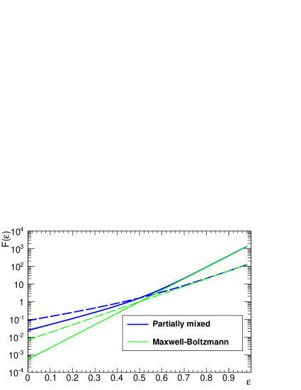
Figure 1: Distribution function proposed in this work, Eq. (19) (thick blue), in comparison with the Maxwell-Boltzmann distribution (thin green). The proposed distribution matches the Maxwell-Boltzmann for $\varepsilon>\mu$, but deviates to another Maxwell-Boltzmann with twice the original “temperature” for $\varepsilon\lesssim\mu$. All curves are for $\mu=0.5$. Continuous curves are for $\beta=15$ and dashed curves for $\beta=10$.

Having determined the distribution function $F\left(\varepsilon\right)$, Eq. (19), we can now calculate the density profiles $\rho\left(r\right)$ of spherically symmetric and isotropic structures generated by the model. In order to do that, we define a dimensionless distance from the center $x=r/a$, a density profile $\tilde{\rho}=\rho/(f_{0}|\phi_{0}|^{3/2})$ and the constant $A=4\pi G\sqrt{|\phi_{0}|}a^{2}f_{0}$, where $a$ is a scale parameter and $G$ is the gravitational constant. In these units, we have

$$\tilde{\rho}\left(\varphi\right)=4\pi\int_{-\infty}^{\varphi}F(\varepsilon)\sqrt{2(\varphi-\varepsilon)}\,\mathrm{d}\varepsilon.$$ (20)

With this relation, we solve Poisson equation $({\nabla^{2}\varphi=-A\tilde{\rho}})$ to determine $\varphi(x)$ and consequently $\tilde{\rho}(x)$. Supposing spherical symmetry, this equation reads

$$\frac{d^{2}\varphi}{dx^{2}}+\frac{2}{x}\frac{d\varphi}{dx}=-A\tilde{\rho}\left(\varphi\right).$$ (21)

We numerically solve this equation with a 4-th order Runge-Kutta algorithm imposing the conditions $\varphi(0)=1$ and ${d\varphi(0)}/{dx}=0$ and fixing $A=10$. The results are shown in Fig. (2), with the density profiles normalized by their values at $x=0.1$.

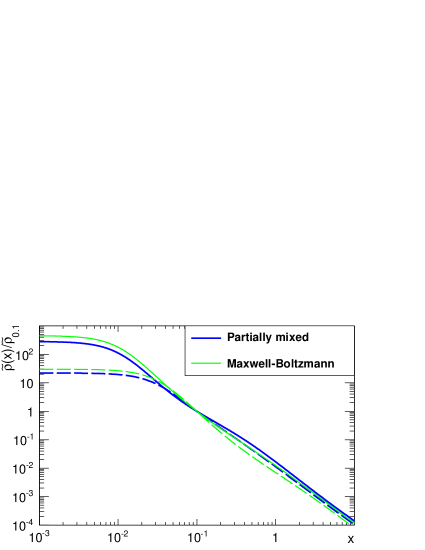
Figure 2: Density profiles generated by our model (thick blue), in comparison with the Isothermal Sphere generated by the Maxwell-Boltzmann distribution (thin green). Values of parameters are the same as in Fig. (1).

We see that our model generates a density profile similar to that of the Isothermal Sphere generated by the Maxwell-Boltzmann distribution: it has a core and it oscillates around $\propto x^{-2}$ in the external regions. This can be more clearly seen in Fig. (3), that shows the density slope $\gamma(x)=-d\ln(\rho)/d\ln(x)$. As is well known, a density profile varying as $\propto x^{-2}$ in the external region generates an infinite mass distribution, in contradiction with the initial constraint of finite mass, and our model is not able, per se, to solve this problem. Instead, we need an extra ingredient related to a correction for the smallness of occupation numbers in the external region, which is discussed in the next section.

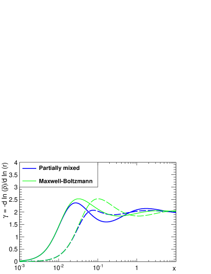
Figure 3: Density slope of the model proposed here (thick blue lines) in comparison with that generated by the Maxwell-Boltzmann distribution (thin green lines). The slope goes to 2 in the external regions, what produces an infinite mass. Parameters as in Fig. (1).

Although not used in the rest of the paper, we also consider the case of introducing an exclusion principle, since it can be tested in other applications. The number of ways to organize indistinguishable particles inside a macro-cell, preventing co-habitation of micro-cells, is given by expression (14). Together with expression (6) for the number of ways to exchange distinguishable particles between macro-cells, it results in

$$W(\{n_{i}\})=\left[\frac{N!}{\left(n_{1}!\right)^{2}\cdots\left(n_{J}!\right)^{2}}\right]\left[\frac{\nu_{1}!}{\left(\nu_{1}-n_{1}\right)!}\cdots\frac{\nu_{J}!}{\left(\nu_{J}-n_{J}\right)!}\right].$$ (22)

Following the same procedures as before, we obtain

$$\ln\left(\frac{\nu_{i}-n_{i}}{n_{i}^{2}}\right)=\lambda m+\eta mE_{i},$$ (23)

from which results

$$F\left(\varepsilon\right)=\frac{1}{2}e^{\beta(\varepsilon-\mu)-k}\left(\sqrt{1+4e^{-\beta(\varepsilon-\mu)+k}}-1\right).$$ (24)

It is interesting to note that, as in Fermi-Dirac versus Bose-Einstein distributions, the only difference between Eqs. (19) and (24) is a $\pm$ sign.

V Correction for small occupation numbers

In the external regions, as the density profile goes to zero, the occupation numbers assume small values, invalidating the use of the Stirling’s approximation, Eq. (9), in deriving the distribution function. With this in mind, Hjorth and Williams (2010) proposed a correction that when applied to the Maxwell-Boltzmann case, gives rise to a distribution function identical to that of King models King (1966), which goes smoothly to zero as $\varepsilon$ approaches a free parameter $\varepsilon_{0}$.

The maximization procedure done in §II can be represented identifying $n!=\Gamma(n+1)$ and remembering the definition of the digamma function $\psi(n)=d\ln\Gamma/dn$. The Stirling’s approximation, Eq. (9), corresponds to ${\psi(n+1)\approx\ln n}$ and the correction proposed by Hjorth and Williams (2010) is given by

$$\psi(n+1)\approx\ln(n+e^{-\gamma}),$$ (25)

where ${\gamma=-\psi(1)\approx 0.57721566}$ is Euler’s constant. This approximation turns out to be excellent, even for very small numbers - see Fig. (1) of Hjorth and Williams (2010).

In fact, if we take this correction for the Maxwell-Boltzmann distribution, as done by Hjorth and Williams (2010), we obtain

$$\ln\left(\frac{\nu_{i}}{n_{i}+e^{-\gamma}}\right)=\lambda m+\eta mE_{i},$$ (26)

which implies that

$$F(\varepsilon)=\left[e^{\beta(\varepsilon-\mu)}-e^{-k-\gamma}\right]\,.$$ (27)

As $F(\varepsilon)$ necessarily goes to zero for some energy, we see that the correction for small numbers already introduces a dependence on $\nu_{i}=e^{k}$, even in the Maxwell-Boltzmann case. If we now impose that the distribution function is zero for $\varepsilon=\varepsilon_{0}$, we have

$$F(\varepsilon)=e^{\beta(\varepsilon_{0}-\mu)}\left[e^{\beta(\varepsilon-\varepsilon_{0})}-1\right],$$ (28)

which corresponds to the King model King (1966).

If we now apply this correction to our model, instead of Eq. (18), we obtain

$$\ln\left(\frac{\nu_{i}+n_{i}-1+e^{-\gamma}}{(n_{i}+e^{-\gamma})^{2}}\right)=\lambda m+\eta mE_{i},$$ (29)

implying that

$$F\left(\varepsilon\right)=\frac{1}{e^{k+\gamma}}\times$$

$$\left\{\frac{1}{2}e^{\beta(\varepsilon-\mu)+\gamma}\left(\sqrt{1+4(e^{k}-1)e^{-\beta(\varepsilon-\mu)}}+1\right)-1\right\},$$ (30)

and again doing $f(\varepsilon_{0})=0$ we have

$$e^{k}=e^{-\gamma}\left(e^{-\beta(\varepsilon_{0}-\mu)-\gamma}-1\right)+1.$$ (31)

In Fig. (4), the thick blue lines show this distribution function for $\beta=(10,15)$, $\mu=0.4$ and with $\varepsilon_{0}=0.03$. Again we see that for decreasing energies, the distribution changes from a Maxwell-Boltzmann to another Maxwell-Boltzmann, but for $\varepsilon\approx\varepsilon_{0}$ it goes to zero. The thin green lines are the King’s models, obtained as a Maxwell-Boltzmann corrected for small occupation numbers.

For a qualitative comparison, we also show the distribution function associated with the Einasto density profile Einasto (1965) - see Appendix A, which describes the details of this calculation, made here for the first time, as far as we know. The two curves shown are for $n=2.5$ and $n=5.0$, representing typical values for galactic and galaxy cluster scale respectively.

Note that the distribution function associated with the Einasto profile, as well as cuspy density profiles in general (see Widrow, 2000) has a “S” shape, with $F(\varepsilon)$ going to zero for small $\varepsilon$ and going to increasing slopes for large $\varepsilon$. It is interesting that the model proposed here, although not presenting exactly the same shape, gives a correction in the same direction, increasing the slope for large values of $\varepsilon$.

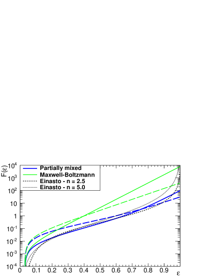
Figure 4: Distribution function corrected for the smallness of occupation numbers, Eq. (30) (thick blue), in comparison with the Maxwell-Boltzmann (also corrected, equivalent to King’s) distribution (thin green). Distribution functions associated with cuspy density profiles (like the Einasto, shown for two values of parameter $n$) have a “S” shape that our model is not quite able to reproduce, although the correction being in the right direction, i.e. increasing the slope of $F(\varepsilon)$ for high $\varepsilon$. All curves are for $\mu=0.4$ and $\varepsilon_{0}=0.03$. Continuous curves are for $\beta=15$ and big dashed curves for $\beta=10$.

As done previously, we calculate the density profiles generated by this function, which are shown in Fig. (5), again normalized by the density at $x=0.1$. We see that now the density profile is steeper than $\propto x^{-2}$ in the external region, and in fact the problem of infinite mass is solved. Also shown are the corrected Isothermal Sphere (King’s model) and the Einasto density profile.

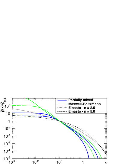
Figure 5: Density profiles generated by the model corrected for small occupation numbers (thick blue), in comparison with that generated by the corrected Maxwell-Boltzmann distribution or King’s model (thin green) and with the Einasto profile. Values or parameters are the same as in Fig. (4).

For completeness, we also show in Fig. (6) the density slope obtained after the correction for small occupation numbers.

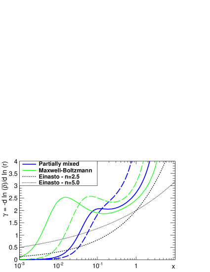
Figure 6: Density slope generated by the model corrected for small occupation numbers (thick blue) in comparison with that generated by the corrected Maxwell-Boltzmann distribution or King’s model (thin green) and with the Einasto profile. Parameters as in Fig. (4).

VI Validity of the Vlasov equation

Let us return to the discussion of the violent relaxation process to see how the association proposed here (between the mixing level and the indistinguishability) can give a clearer meaning to an important hypothesis assumed in the deduction of the Vlasov equation.

Intuitively, one expects that during violent relaxation, a process that starts far from equilibrium, the total field varies in a very complex way, producing chaotic motions and driving the system to an equilibrium (or stationary) state. In fact, as pointed out in Merritt and Valluri (1996), the presence of chaotic motions combined with the rapid approach to a stationary state observed in numerical simulations seems to indicate this effect. However the Vlasov equation is reversible in time, which is incompatible with a process driving the system to an equilibrium (or relaxed) state characterized by a maximum entropy. In fact, Tremaine et al. (1986) have shown that if the system is described by Eq. (1), there is no upper limit for the entropy associated with any convex function $C(f)$, in particular for the Boltzmann entropy, represented by $C(f)=f\ln f$. The standard argument to solve this problem is that the evolution to an equilibrium state is given in a coarse-grained sense, while the Vlasov equation concerns the fine-grained distribution function.

The deduction of the equation governing the evolution of the one-particle distribution function $f$ is usually done starting from the Liouville equation. It states that an isolated system composed of $N$ particles collectively represented by the $N$-particle joint distribution function $f^{(N)}\left(\bf{x_{1},p_{1},...,x_{N},p_{N}},t\right)$ necessarily respects (see Liboff, 2003)

$$\frac{df^{(N)}}{dt}=0.$$ (32)

This equation can be statistically interpreted as the evolution of the system as a whole being smooth, free of sudden changes, which is adequate since it describes an isolated system (by definition free of external influences), whose particles move according to Hamilton equations.

The next step to obtain the equation for the one-particle distribution $f$ is the construction of the so-called BBGKY hierarchy (see Lifshitz and Pitaevskii, 1980; Binney and Tremaine, 2008; Saslaw, 1987), and it involves some extra assumptions. The first one is the symmetry of $f^{(N)}\left(\bf{x_{1},p_{1},...,x_{N},p_{N}},t\right)$ relative to changes of coordinates and momenta of the particles. This makes the phase-space averaged contribution of each particle to the total force exerted on the test particle to be the same, implying Eq. (53) - see Appendix C. The second hypothesis is that of molecular chaos, i.e., that the two-particle distribution function is just the product of two one-particle distribution functions, the correlations being negligible, as is expressed by Eq. (56). With these two hypothesis, one obtains Vlasov equation, Eq. (1).

Far from being just a calculation strategy, these assumptions have a deep statistical meaning, and without them it is not possible (to the best of our knowledge) to obtain the Vlasov equation. The symmetry of $f^{(N)}$ is commonly treated as a direct consequence of the assumption of identical particles (see Binney and Tremaine, 2008; Saslaw, 1987). However, there is no mechanical principle that guarantees this symmetry. Instead, it is an extra hypothesis, with important statistical content. In our context it is equivalent to treating particles not only as identical but as indistinguishable and, according to the criterion discussed in §III, it refers to the possibility of all particles to visit the same regions of phase-space. As already pointed out by Saslaw (1987), the BBGKY hierarchy was developed to describe molecules in fluids and ions in plasmas close to equilibrium. These systems are very different from a self-gravitating system during violent relaxation, which is a phenomenon that starts far from equilibrium. Besides, as discussed in §I, self-gravitating systems are not able to fully mix the phase-space, or at least are expected to be much less effective in doing so than plasmas or fluids in laboratory.

From this discussion, it seems that there is no reason to suppose that the symmetry of $f^{(N)}$ is a valid hypothesis during violent relaxation. Besides that, the correlations in situations far from equilibrium may be large (see Saslaw, 2008), which also may contradict the assumption of molecular chaos, Eq. (56). Thus the Vlasov equation does not seem to be valid during this process. In fact, as pointed out by Kandrup (1998), the relation between the full N-body problem and the associated transport equation (presumably the Vlasov equation) is far more complicated than usually assumed. Although we do not propose any concrete alternative to Vlasov equation, we expect that during violent relaxation the one-particle distribution $f$ must be described by a full transport equation,

$$\frac{\partial f}{\partial t}+{\bf v}\cdot\frac{\partial f}{\partial{\bf r}}-\nabla\phi\cdot\frac{\partial f}{\partial{\bf v}}=L[f],$$ (33)

where $L[f]$ is a stochastic term (see Kandrup (1980)) related to chaotic changes of the potential.

This can be so even if we can neglect 2-body interactions. The idea of the “collisional” term in the Boltzmann equation is associated, not exactly with collisions, but to any stochastic process that suddenly changes the probability flux of the test particle (see Lifshitz and Pitaevskii, 1980). In ideal gases, these processes are realized by the collisions, but for systems with long-range interactions, it can be a chaotically time changing mean field. As the distribution function $f$ carries information about the system as a whole, the long-range interactions transmit the small perturbations of all particles to the test particle.

The above discussion is relevant for what we have proposed in this paper for two reasons: first, it reinforces our expectation that self-gravitating systems can achieve a stationary state as a consequence of going through irreversible processes, without the need to advocate the coarse-grained sense usually attributed to this evolution Tremaine et al. (1986). In other words, a real “arrow of time” is introduced if the Vlasov equation is not valid during the violent relaxation process and the stationary state can be predicted by the old strategy of maximizing the complexions, i.e. the number of possible micro-configurations given the constraints of the problem. Secondly, it is questionable whether or not the Vlasov equation should imply an exclusion principle constraint (as discussed in §II). In case this equation is not valid during violent relaxation, there would be even less reason to impose such constraint. That is why we did not impose in our analysis the exclusion principle proposed by Lynden-Bell Lynden-Bell (1967).

VII Conclusion

We propose a new criterion to choose between distinguishability and indistinguishability, namely the level of mixing in phase-space. According to this, in systems that do not have enough time to completely mix phase elements, particles in well mixed regions must be treated as indistinguishable and particles in poorly mixed regions must be treated as distinguishable. This criterion is consistent with the standard classification of ideal gases as being made of indistinguishable particles and of crystals as being made of distinguishable particles. However it opens new perspectives on the classification of systems of macroscopic constituents like colloids and self-gravitating systems. It also provides a solution to the Gibbs paradox without the need of arguments related to the quantum nature of particles (see Appendix B).

Violent relaxation is known to be incomplete, in the sense that the particles (or stars) cannot explore all regions of phase-space before the achievement of a stationary state. Thus the model proposed here can represent a solution to this problem, explicitly translating this incompleteness in the combinatorial analysis. According to Kandrup et al. (1993), during violent relaxation the particles “forget” the positions and velocities but keep the initial order in their energies. We express this fact treating particles as indistinguishable for exchanges inside a macro-cell (that defines an energy value) but as distinguishable for exchanges between macro-cells.

The result is a new distribution function that tends to the Maxwell-Boltzmann distribution for high energies, but deviates to another Maxwell-Boltzmann distribution with twice the original “temperature” for low energies.

The density profiles generated by this distribution function resemble those predicted by the Maxwell-Boltzmann distribution, the Isothermal Sphere. As so, they vary as $\propto x^{-2}$ in the external regions, yielding an infinite mass system. However, in the external regions the occupation numbers are small, invalidating the use of Stirling’s approximation. Using the correction proposed by Hjorth and Williams (2010), we obtain a distribution function that goes to zero for an energy fixed by a parameter $\varepsilon_{0}$. The density profile generated by this corrected distribution function is steeper in the external region, effectively solving the infinite mass problem.

It is interesting to note that the corrected distribution function resembles the “S” shape of the distribution associated with the Einasto profile, or at least provides a correction in the right direction. The high energy part of this function determines the behavior of the density profile in the inner region Widrow (2000) and our model seems to go in the right direction to generate high densities that could mimic a cuspy profile.

The new distribution function obtained in this work can be tested and used in several astrophysical applications. For example, the resulting density profile can be fit to gravitational lensing data from galaxy clusters, as done for other models in Beraldo e Silva et al. (2013). Another direct test can be made with data from rotation curves of spiral galaxies. On smaller scales, analyses of the density profile can also be made from optical data of globular clusters. A caveat that we should point out is that the dissipative nature of the baryon collapse also affects the density profile of astrophysical objects Martizzi et al. (2012), which complicates the comparison with observational data.

The velocity distribution associated to the model can be tested by fitting to the simulated data of structure formation, as done by Vogelsberger et al. (2009); Lisanti et al. (2011) to test different models. In the analysis of direct detection experiments such as the XENON Xenon100 Collaboration et al. (2012) and CDMS Agnese et al. (2014) projects, the velocity distribution is an important ingredient for the predicted event rate associated to different dark matter particles and the model proposed here can be of some utility in this context. Another possible application is in mass modeling methods such as MAMPOSSt Mamon et al. (2013), in which the distribution of tracers in projected phase space is used to determine the total density and anisotropy profiles, starting from the assumption of some 3D velocity distribution.

We also considered the possibility of preventing co-habitation in micro-cells keeping the same criterion for distinguishability as before, obtaining another distribution function, differing from the first by a $\pm$ sign. Both distribution functions obtained here can be of some importance for other phenomena far from equilibrium.

Finally, we showed how the association between the mixing level and indistinguishability gives a physical meaning for the assumption of symmetry of the N-particle distribution function $f^{(N)}$. This assumption is equivalent to treat particles as indistinguishable, which is a stronger assumption than treating them as identical and, according to the criterion proposed here, it is equivalent to the assumption that all particles have access to the same regions of phase-space, i.e. that the system is completely mixed. Since it is well known that such mixing is not complete in self-gravitating systems during violent relaxation, this suggests that the symmetry hypothesis is not adequate and thus the Vlasov equation is not necessarily valid during this process.

Appendix A Einasto distribution function

The Einasto density profile was proposed in the 60’s to describe the surface brightness of elliptical galaxies and recently has been used to fit data of simulated Navarro et al. (2004); Merritt et al. (2005) and observed structures in the galactic and galaxy cluster scales Beraldo e Silva et al. (2013), giving results better than NFW in many cases. In fact, it can mimic the cuspy density profile described by NFW, despite being finite at the origin. The profile is given by

$$\tilde{\rho}(x)=\exp\left\{-2n(x^{1/n}-1)\right\}.$$ (34)

The associated potential is given by Retana-Montenegro et al. (2012):

$$\varphi(x)=-\frac{\phi(x)}{|\phi(0)|}=\frac{\Gamma(3n)}{\Gamma(2n)}\frac{1}{(2n)^{n}x}\times$$

$$\left[1-\frac{\Gamma(3n,2nx^{1/n})}{\Gamma(3n)}+(2n)^{n}x\frac{\Gamma(2n,2nx^{1/n})}{\Gamma(3n)}\right],$$ (35)

where $\Gamma(a,x)$ is the (upper) incomplete gamma function. The distribution function $F(\varepsilon)$ can be obtained from Eq. (20) through an Abel transform (see Binney and Tremaine, 2008):

$$F(\varepsilon)=\frac{1}{\sqrt{8}\pi^{2}}\left[\int_{0}^{\varepsilon}\,\frac{d^{2}\tilde{\rho}}{d\varphi^{2}}\frac{d\varphi}{\sqrt{\varepsilon-\varphi}}+\frac{1}{\sqrt{\varepsilon}}\left(\frac{d\tilde{\rho}}{d\varphi}\right)_{\varphi=0}\right],$$ (36)

where the second term in the square bracket is zero for the Einasto profile. Following Widrow (2000), we use Eqs. (34) and (35) and solve the integral above numerically. The results are shown in Fig. (4) for two values of $n$.

Appendix B The Gibbs paradox

Since the beginning of the development of statistical mechanics up to the present days, the Gibbs paradox has brought many discussions and attempts of solution, definite for ones and unsatisfactory for others. It can be described in various forms, in particular as follows Jaynes (1992): an enclosure volume $V$ is divided by a wall into two volumes $V_{1}$ and $V_{2}$ filled respectively with $N_{1}$ and $N_{2}$ molecules with mass $m$ of the same gas subject to the same conditions of pressure and temperature. Assuming that the particles are distinguishable, the initial number of micro-states compatible with the macro-state 1, the same being for 2, is:

$$W_{I}^{1}=\int d^{3}\vec{r_{1}}...\int d^{3}\vec{r_{N_{1}}}\int d^{3}\vec{p_{1}}...\int d^{3}\vec{p_{N_{1}}}\Rightarrow$$ (37)

$$W_{I}^{1}=V_{1}^{N_{1}}\cdot\frac{\left(2\pi m\right)^{\frac{3N_{1}}{2}}}{\Gamma\left(\frac{3N_{1}}{2}\right)}E_{1}^{\frac{3N_{1}}{2}}$$ (38)

We calculate the entropy as $S_{I}^{1}=\ln W_{I}^{1}$ (the same for 2) and the total entropy is $S_{I}=S_{I}^{1}+S_{I}^{2}$. Setting $f=N_{1}/N=V_{1}/V=E_{1}/E$, and applying the thermodynamic limit $\left(N\rightarrow\infty\right)$, the entropy per particle is

$$\frac{S_{I}}{N}=s_{I}=f\ln f+\left(1-f\right)\ln\left(1-f\right)+$$

$$+\ln V+\frac{3}{2}\ln u+\frac{3}{2}\ln\left(\frac{4\pi}{3}m\right)+\frac{3}{2},$$ (39)

where $u=E/N$ is the energy per particle and it was used the Stirling’s approximation, $\ln N!\approx N\ln N-N$.

After removing the wall and considering the system as whole, recalculation of the total number of micro-states gives

$$W_{F}=V^{N}\cdot\frac{\left(2\pi m\right)^{\frac{3N}{2}}}{\Gamma\left(\frac{3N}{2}\right)}E^{\frac{3N}{2}},$$ (40)

and it follows that

$$s_{F}=\ln V+\frac{3}{2}\ln u+\frac{3}{2}\ln\left(\frac{4\pi}{3}m\right)+\frac{3}{2}.$$ (41)

Thus, the entropy before and after removing the division differ by

$$\Delta s=-\left[f\ln f+\left(1-f\right)\ln\left(1-f\right)\right].$$ (42)

In the particular case of equal volumes we have

$$\Delta s=\ln 2.$$ (43)

Therefore, if we consider that the gas particles are distinguishable, as classically assumed, we conclude that there was an increase in entropy, which does not agree with the fact that there is no macroscopic change in the system. Hence the paradox.

If on the other hand we assume that the particles are indistinguishable, we have to divide the number of complexions obtained previously by the number of permutations of the $N_{1}$, $N_{2}$ or $N$ particles. Thus,

$$W_{I}^{1}=\frac{1}{N_{1}!}\int d^{3}\vec{r_{1}}...\int d^{3}\vec{r_{N_{1}}}\int d^{3}\vec{p_{1}}...\int d^{3}\vec{p_{N_{1}}},$$ (44)

the same for 2. Following the same steps as in the previous case, we arrive at

$$s_{I}=\ln v+\frac{3}{2}\ln u+\frac{3}{2}\ln\left(\frac{4\pi}{3}m\right)+\frac{5}{2},$$ (45)

where $v=V/N$. Again, removing the wall, the phase space and the entropy become

$$W_{F}=\frac{1}{N!}\int d^{3}\vec{r_{1}}...\int d^{3}\vec{r_{N}}\int d^{3}\vec{p_{1}}...\int d^{3}\vec{p_{N}}$$ (46)

and

$$s_{F}=\ln v+\frac{3}{2}\ln u+\frac{3}{2}\ln\left(\frac{4\pi}{3}m\right)+\frac{5}{2}\Rightarrow$$ (47)

$$\Delta s=0.$$ (48)

Thus, removal of the wall does not produce increase in entropy (which is within our expectations), once we consider that the particles are indistinguishable, the justification being traditionally associated with the quantum behavior of the gas molecules.

On the other hand, according to this standard interpretation, a system with particles almost identical (with arbitrarily similar mass, for example) would still present the same increase in entropy. This discontinuity, passing from identical to arbitrarily similar particles, still cannot be explained if the indistinguishability depends on the particles being strictly identical.

Furthermore, appealing to quantum mechanics to solve Gibbs paradox is deemed unsatisfactory to some authors Versteegh and Dieks (2011), because it should not be necessary to use quantum arguments in a strictly classical conceptual problem. In other terms, it is not an experimental evidence of need for quantum physics, but a conceptual inconsistency internal to classical physics, which should be solved in classical terms.

Appendix C BBGKY Hierarchy

Let a system with $N$-particles be described by the Hamiltonian

$$H=\displaystyle\sum_{a=1}^{N}\left[\frac{{\bf p}_{a}^{2}}{2m}+\displaystyle\sum_{b=a+1}^{N}U\left(|{\bf r}_{a}-{\bf r}_{b}|\right)\right],$$ (49)

where $U\left(|{\bf r}_{a}-{\bf r}_{b}|\right)$ is the potential energy. The evolution of the $N-$particle distribution function $f^{(N)}$ is governed by Liouville equation [Eq. (32)]. With the help of Hamilton equations, it reads

$$\frac{\partial f^{(N)}}{\partial t}+\displaystyle\sum_{a=1}^{N}\left(\frac{\partial f^{(N)}}{\partial{\bf r}_{a}}\frac{{\bf p}_{a}}{m}-\frac{\partial f^{(N)}}{\partial{\bf p}_{a}}\displaystyle\sum_{b=a+1}^{N}\frac{\partial U_{ab}}{\partial{\bf r}_{a}}\right)=0,$$ (50)

where $U_{ab}=U\left(|{\bf r}_{a}-{\bf r}_{b}|\right)$.

We want to derive the equation for the one-particle distribution $f$. This function is not to be interpreted as describing the evolution of some specific particle, but that of a test particle randomly chosen. In this sense, it keeps statistical information about the system as a whole, even-though referring to coordinates of one particle. Also we normalize the one-particle distribution $f$ taking into account all the permutations between the $(N-1)$ remaining particles Liboff (2003):

$$f=\frac{N!}{(N-1)!}\int f^{(N)}(\Gamma_{1},\dots,\Gamma_{N})d\Gamma_{2}\dots d\Gamma_{N},$$ (51)

where $d\Gamma_{i}=d{\bf r}_{i}d{\bf p}_{i}$. Following standard steps we integrate Eq. (50) in $d\Gamma_{2}\dots d\Gamma_{N}$, obtaining

$$\frac{(N-1)!}{N!}\left(\frac{\partial f}{\partial t}+\frac{\partial f}{\partial{\bf r}_{1}}\frac{{\bf p}_{1}}{m}\right)=$$

$$=\frac{\partial}{\partial{\bf p}_{1}}\displaystyle\sum_{b=2}^{N}\int f^{(N)}\frac{\partial U_{1b}}{\partial{\bf r}_{1}}d\Gamma_{2}\dots d\Gamma_{N}.$$ (52)

The integral in the right hand side represents the force exerted on the test particle by each one of the other particles, averaged over the phase space region occupied by each of them. Now comes the first strong assumption: if we suppose that the $N$-particles distribution $f^{(N)}$ is symmetric in the particles coordinates $\Gamma_{1}\dots\Gamma_{N}$, the averaged contribution to the total force exerted on the test particle is equal for each one, and we have

$$\displaystyle\sum_{b=2}^{N}\int f^{(N)}\frac{\partial U_{1b}}{\partial{\bf r}_{1}}d\Gamma_{2}\dots d\Gamma_{N}=$$

$$=(N-1)\int f^{(N)}\frac{\partial U_{12}}{\partial{\bf r}_{1}}d\Gamma_{2}\dots d\Gamma_{N}.$$ (53)

Accordingly, we define the two-particles distribution function as

$$f^{(2)}=\frac{N!}{(N-2)!}\int f^{(N)}(\Gamma_{1},\dots,\Gamma_{N})d\Gamma_{3}\dots d\Gamma_{N},$$ (54)

thus obtaining

$$\frac{\partial f}{\partial t}+\frac{\partial f}{\partial{\bf r}_{1}}\frac{{\bf p}_{1}}{m}=\int\frac{\partial U_{12}}{\partial{\bf r}_{1}}\frac{\partial f^{(2)}(t,\Gamma_{1},\Gamma_{2})}{\partial{\bf p}_{1}}d\Gamma_{2}.$$ (55)

Now comes the second strong assumption, that of molecular chaos, according to which

$$f^{(2)}(t,\Gamma_{1},\Gamma_{2})=f(t,\Gamma_{1})f(t,\Gamma_{2}),$$ (56)

and we finally obtain the Vlasov equation:

$$\frac{\partial f}{\partial t}+\frac{\partial f}{\partial{\bf r}}{\bf v}-\frac{\partial\phi}{\partial{\bf r}}\frac{\partial f}{\partial{\bf v}}=0,$$ (57)

where we used ${\bf p}=m{\bf v}$ and the mean potential $\phi({\bf r})$ is given by

$$\phi({\bf r},t)=\frac{1}{m}\int U(|{\bf r}-{\bf r}^{\prime}|)f({\bf r}^{\prime},{\bf p}^{\prime},t)d{\bf r}^{\prime}d{\bf p}^{\prime}.$$ (58)

References

- Padmanabhan (1990) T. Padmanabhan, Physics Reports 188 (1990).
- Binney and Tremaine (2008) J. Binney and S. Tremaine, Galactic Dynamics - Second Edition (Princeton University Press, 2008).
- Hénon (1964) M. Hénon, Annales d’Astrophysique 27, 83 (1964).
- King (1966) I. R. King, The Astronomical Journal 71, 64 (1966).
- Lynden-Bell (1967) D. Lynden-Bell, MNRAS 136, 101 (1967).
- Navarro et al. (1997) J. F. Navarro, C. S. Frenk, and S. D. M. White, ApJ 490, 493 (1997).
- Navarro et al. (2004) J. F. Navarro, E. Hayashi, C. Power, A. R. Jenkins, C. S. Frenk, S. D. M. White, V. Springel, J. Stadel, and T. R. Quinn, MNRAS 349, 1039 (2004).
- Merritt et al. (2005) D. Merritt, J. F. Navarro, A. Ludlow, and A. Jenkins, ApJ 624, L85–L88 (2005).
- Merritt et al. (2006) D. Merritt, A. W. Graham, B. Moore, J. Diemand, and B. Terzić, AJ 132, 2685 (2006).
- Umetsu et al. (2011) K. Umetsu, T. Broadhurst, A. Zitrin, E. Medezinski, D. Coe, and M. Postman, ApJ 738, 41 (2011).
- Beraldo e Silva et al. (2013) L. Beraldo e Silva, M. Lima, and L. Sodré, MNRAS 436, 2616 (2013).
- Pontzen and Governato (2014) A. Pontzen and F. Governato, Nature (London) 506, 171 (2014).
- Spergel and Steinhardt (2000) D. N. Spergel and P. J. Steinhardt, Physical Review Letters 84, 3760 (2000).
- Williams (2012) L. L. R. Williams, MNRAS 423 (2012).
- Shu (1978) F. H. Shu, ApJ 225, 83 (1978).
- Madsen (1987) J. Madsen, ApJ 316, 497 (1987).
- Shu (1987) F. H. Shu, ApJ 316, 502 (1987).
- Efthymiopoulos et al. (2007) C. Efthymiopoulos, N. Voglis, and C. Kalapotharakos, in Topics in Gravitational Dynamics, Lecture Notes in Physics, Vol. 729, edited by D. Benest, C. Froeschle, and E. Lega (Springer Berlin Heidelberg, 2007) pp. 297–389.
- Bindoni and Secco (2008) D. Bindoni and L. Secco, NewAR 52, 1 (2008).
- Hjorth and Williams (2010) J. Hjorth and L. R. Williams, ApJ 722, 851 (2010).
- Pontzen and Governato (2013) A. Pontzen and F. Governato, MNRAS 430, 121 (2013), arXiv:1210.1849 [astro-ph.CO] .
- Saslaw (1987) W. C. Saslaw, Gravitational Physics of Stellar and Galactic Systems, Cambridge University Press (1987).
- Lichtenberg and Lieberman (1992) A. J. Lichtenberg and M. A. Lieberman, Regular and Chaotic Dynamics, 2nd ed., Applied Mathematical Sciences No. 38 (Springer-Verlag, New York, NY, 1992).
- Chavanis (2006) P.-H. Chavanis, Physica A 365, 102 (2006).
- Merritt (2005) D. Merritt, Annals NY Acad. of Sciences 1045, 3 (2005).
- Kull et al. (1996) A. Kull, R. A. Treumann, and H. Boehringer, Astrophysical Journal Letters 466, L1 (1996).
- Tolman (1979) R. C. Tolman, The principles of statistical mechanics, edited by Dover (Dover, 1979).
- Huang (1987) K. Huang, Statistical Mechanics, 2nd Edition, Wiley-VCH (1987).
- Landau and Lifshitz (1980) L. D. Landau and E. M. Lifshitz, Statistical Physics, Part 1. (Butterworth–Heinemann, 1980).
- Schönberg (1952) M. Schönberg, Il Nuovo Cimento 9, 1139 (1952).
- Schönberg (1953) M. Schönberg, Il Nuovo Cimento 10, 419 (1953).
- Swendsen (2006) R. H. Swendsen, Am. J. Phys. 74 (2006).
- de Muynck and van Liempd (1986) W. M. de Muynck and G. P. van Liempd, Synthese 67, 477 (1986).
- Versteegh and Dieks (2011) M. A. M. Versteegh and D. Dieks, Am. J. Phys. 79(7), 741 (2011).
- Saslaw (1969) W. C. Saslaw, MNRAS 143, 437 (1969).
- Teles et al. (2010) T. N. Teles, Y. Levin, R. Pakter, and F. B. Rizzato, J. Stat. Mech. 05, 05007 (2010).
- Teles et al. (2011) T. N. Teles, Y. Levin, and R. Pakter, MNRAS 417, L21–L25 (2011).
- Kandrup et al. (1993) H. E. Kandrup, M. E. Mahon, and H. Smith, Jr., Astronomy and Astrophysics 271, 440 (1993).
- Einasto (1965) J. Einasto, Trudy Astrofizicheskogo Instituta Alma-Ata 5, 87 (1965).
- Widrow (2000) L. M. Widrow, ApJS 131, 39 (2000).
- Merritt and Valluri (1996) D. Merritt and M. Valluri, ApJ 471, 82 (1996).
- Tremaine et al. (1986) S. Tremaine, M. Henon, and D. Lynden-Bell, MNRAS 219, 285 (1986).
- Liboff (2003) R. L. Liboff, Kinetic Theory: Classical, Quantum and Relativistic Descriptions, 3rd edition (2003).
- Lifshitz and Pitaevskii (1980) E. M. Lifshitz and L. P. Pitaevskii, Physical Kinetics (Butterworth–Heinemann, 1980).
- Saslaw (2008) W. C. Saslaw, The Distribution of the Galaxies, Cambridge University Press (2008).
- Kandrup (1998) H. E. Kandrup, Annals NY Academy of Sciences 848, 28 (1998).
- Kandrup (1980) H. E. Kandrup, Physics Reports 63, 1 (1980).
- Martizzi et al. (2012) D. Martizzi, R. Teyssier, B. Moore, and T. Wentz, MNRAS 422, 3081 (2012).
- Vogelsberger et al. (2009) M. Vogelsberger, A. Helmi, V. Springel, S. D. M. White, J. Wang, A. Frenk, Carlos S.; Jenkins, A. Ludlow, and J. F. Navarro, MNRAS 395, 797 (2009).
- Lisanti et al. (2011) M. Lisanti, L. E. Strigari, J. G. Wacker, and R. H. Wechsler, PRD 83, 023519 (2011).
- Xenon100 Collaboration et al. (2012) Xenon100 Collaboration, E. Aprile, K. Arisaka, F. Arneodo, et al., Astroparticle Physics 35, 573 (2012), arXiv:1107.2155 [astro-ph.IM] .
- Agnese et al. (2014) R. Agnese, A. J. Anderson, M. Asai, et al., Physical Review Letters 112, 241302 (2014), arXiv:1402.7137 [hep-ex] .
- Mamon et al. (2013) G. A. Mamon, A. Biviano, and G. Moué, MNRAS 429, 3079 (2013).
- Retana-Montenegro et al. (2012) E. Retana-Montenegro, E. van Hese, G. Gentile, M. Baes, and F. Frutos-Alfaro, A&A 540, A70 (2012).
- Jaynes (1992) E. T. Jaynes, in Maximum-Entropy and Bayesian Methods (Kluwer Academic: Dordrecht, 1992) pp. 1–22.