Forecasting the 2013–2014 Influenza Season using Wikipedia

Abstract

Infectious diseases are one of the leading causes of morbidity and mortality around the world; thus, forecasting their impact is crucial for planning an effective response strategy. According to the Centers for Disease Control and Prevention (CDC), seasonal influenza affects between 5% to 20% of the U.S. population and causes major economic impacts resulting from hospitalization and absenteeism. Understanding influenza dynamics and forecasting its impact is fundamental for developing prevention and mitigation strategies.

We combine modern data assimilation methods with Wikipedia access logs and CDC influenza-like illness (ILI) reports to create a weekly forecast for seasonal influenza. The methods are applied to the 2013–2014 influenza season but are sufficiently general to forecast any disease outbreak, given incidence or case count data. We adjust the initialization and parametrization of a disease model and show that this allows us to determine systematic model bias. In addition, we provide a way to determine where the model diverges from observation and evaluate forecast accuracy.

Wikipedia article access logs are shown to be highly correlated with historical ILI records and allow for accurate prediction of ILI data several weeks before it becomes available. The results show that prior to the peak of the flu season, our forecasting method projected the actual outcome with a high probability. However, since our model does not account for re-infection or multiple strains of influenza, the tail of the epidemic is not predicted well after the peak of flu season has past.

Keywords: Disease forecasting, Wikipedia data, Influenza, Data assimilation, Ensemble Kalman filter

Author Summary

We use modern methods for injecting current data into epidemiological models in order to offer a probabilistic evaluation of the future influenza state in the U.S. population. This type of disease forecasting is still in its infancy, but as these methods become more developed it will allow for increasingly robust control measures to react to and prevent large disease outbreaks. While weather forecasting has steadily improved over the last half century and become ubiquitous in modern life, there is surprisingly little work on infectious disease forecasting. Although there has been a great deal of work in modeling disease dynamics, these have seldom been used to generate a probabilistic description of expected future dynamics, given current public health data. Moreover, the mechanism to update expected disease outcomes as new data becomes available is just beginning to receive attention from the public health community. Using CDC influenza like illness reports and digital monitoring sources, such as observations of Wikipedia access logs, we are now at a point where forecasting for the influenza season can be brought inline with our advancements in weather prediction.

1 Introduction

Despite preventative efforts and educational activities for seasonal influenza, thousands of people are affected every year and many die, resulting in a significant public health and economic burden for the U.S. population [1, 22, 26]. The CDC monitors influenza burden by collecting information from volunteer public health departments at the state and local level [10]. Data are then used for planning and mitigation activities based on what is believed to be the current state of influenza throughout the U.S. [2, 29]. These rough estimates can lead to significant over- or under-preparation for any given flu season since little modeling of influenza dynamics is used to extrapolate from the current state of influenza to the state of influenza for the remaining season.

The capability for real-time forecasting of events, such as influenza dynamics, with quantified uncertainty, has been crucial for numerous major advances across the spectrum of science [32, 20, 16]. However, this capability is still in its infancy in the field of public health. For more complete literature reviews on the field we refer the reader to [14, 41]. Briefly, we present the literature on epidemic forecasting influencing this work, all of which rely on a Bayesian viewpoint to adjust an underlying disease model given incoming observations [8]. First, disease forecasting methods that use data to parameterize an underlying causal model of disease can use either sequential Monte Carlo type methods [7, 40, 55, 43, 51, 31, 6] or ensemble methods [48, 49, 15, 36]. Some work has been done on comparing the two methods [54, 50]. There are also several works of more statistical nature [39, 42, 38, 13, 47, 9], one that relies on a pure Kalman filter [11], and one [45] that uses variational assimilation methods. Of these works, the majority tune a differential equation based compartmental disease model [50, 31, 45, 51, 54, 49, 55, 48, 7]. However, some forecasts have been formed using agent based simulations [6, 40, 13] or spatial models [36, 15].

Each of these examples rely on defining a prior distribution for the parameterization and initialization of the underlying model. However, the methods to arrive at this prior are usually ad hoc and based on beliefs about the ranges for the parameters. It is therefore difficult to see how these methods may be applied to a general disease model given historic observations in the presence of model error. In this work, we outline a method for defining a prior parameterization/initialization that can be generalized to any data set pertaining to disease spread and disease model.

With the exception of reference [45], the aforementioned methods only use the most recent observation to update the epidemic model. This can lead to problems in determination of the underlying model parameters since the dynamic trends of the data are not considered during the model adjustment. We use an ensemble Kalman smoother approach that is more sensitive to the underlying dynamics of the data timeseries.

Another difficulty during data assimilation is that, in the adjustment of the current model state, conditions such as the population in each epidemic category summing to the total population are often disrupted. Moreover, since the model state is adjusted each time an observation is made, the forecast epidemic curve may not represent any single realization of the epidemic model. This makes it difficult to judge systematic model error and thus identify specific areas to where the model may be improved. To remedy this difficulty in our assimilation scheme, we only adjust the model’s parameterization and initialization. Therefore, each of our forecasts represent a realization of the model.

In November of 2013, the CDC launched the Predict the Influenza Season Challenge competition to evaluate the growing capabilities in disease forecasting models that use digital surveillance data [12]. The competition asked entrants to forecast the timing, peak, and disease incidence of the 2013-2014 influenza season using Twitter or other Internet data to supplement ILI weekly reported data. The work described in this paper was conducted as an entry for this competition.

The significant obstacles to accurately predicting the spread of diseases include:

• Data pertaining to disease dynamics is difficult to obtain in real time for many diseases. When data is available, such as ILI data, it can be difficult to quantify its relation to the actual number of disease (e.g. influenza) cases. Also, when using recent data, the underreporting and reporting delays lead to additional uncertainties and a constantly updated database.

• Data assimilation algorithms must be developed for dynamically incorporating the incidence data into mathematical transmission models. Although these methodologies have been developed for atmospheric sciences (i.e., weather prediction) models, the epidemiology community has only recently begun apply these approaches to transmission models.

Reliable forecasts of influenza dynamics in the U.S. cannot be obtained without consistently updated public health observations pertaining to flu [19]. It is necessary to have a historical record of these observations in order to asses the relation between the forecasting model and the data source. We used the well established public health observation system for influenza in the U.S., the influenza-like illness (ILI) network [2, 43]. This network has been in place for over a decade and reports the percentage of patients in the U.S. seen for ILI each week. ILI data provide an informative depiction of the state of influenza in the U.S. each week. However, it represents a limited syndromic observation of people who seek medical attention each week [29]. This is different than what our disease model represents, which is the dynamics of the proportion of the population currently infected. A further drawback is related to the bureaucratic hierarchy of the ILI system; there is a 1–2 week lag present in data availability.

The addition of other data sources that provide different estimates for influenza incidence can add to the robustness of this data stream [25, 37, 27, 44, 33]. In this work, we use Wikipedia access logs for articles highly correlated with influenza prevalence, as measured by ILI, to improve our knowledge of the current influenza incidence in the U.S. The rationale for using the Wikipedia access logs was thoroughly explored in reference [25].

Influenza forecasting must provide two things in order to inform public health policy: 1) the expected future influenza dynamics and 2) the likelihood of observing dynamics deviating from this expectation. These two properties must be informed by both the inherent model dynamics and current observations of flu. Fortunately for epidemiologists, the problem of turning a deterministic mathematical model into a probabilistic forecast using observed data has a long history in the areas of climatology, meteorology, and oceanography [32, 20, 16]. We demonstrate that one of these techniques, the ensemble Kalman smoother, can be used to iteratively update a distribution of the influenza model’s initial conditions and parameterizations. An advantage of this particular technique is that it retains information about when the model dynamics systematically diverge from the dynamics of observations. Therefore, it is clear where to focus efforts to improve the forecasting power of the model.

After outlining the general forecast methodology, we describe the details of our data sources and model, the technique used to estimate a prior forecast, our data assimilation technique, and our measure of forecast accuracy. We then present an application of our methods to forecasting the 2013–2014 influenza season in the results section, and conclude with a summary of our approach and suggestions for future improvements.

2 Methods

Data and Model

Our goal is to forecast future U.S. influenza dynamics using CDC ILI data and Wikipedia access log data. On one hand, the ILI data represent the ground truth that we attempt to forecast and use to train our models. The Wikipedia data, on the other hand, has the potential to provide information about the current state of influenza.

The CDC’s ILI data represent the collection of outpatient data from over 3,000 hospitals and doctors’ offices across the U.S. Each week, these locations report the total number of patient visits and the number of those visits that were seen for ILI defined as fever (temperature $\geq 100^{\circ}$F) and a cough or sore throat without a known cause other than influenza. Since 2003, these data have been collected weekly, year-round. Clearly, these data are related to the proportion of the U.S. population infected with influenza. However, it does not contain information about the proportion of the population that does not seek treatment and the proportion of people seeking treatment who have flu symptoms but not the flu virus.

ILI outpatient data make up one portion of the CDC’s influenza surveillance capabilities. The outpatient data described above are also divided into 10 Health and Human Services (HHS) regions. In collaboration with the World Health Organization (WHO), U.S. influenza vaccination coverage and virological strain data are also collected, we only use the total U.S. ILI data. For a complete overview of the CDC’s influenza surveillance programs we refer the reader to [2, 43].

As mentioned above, there is a 1–2 week delay between a patient seeing a doctor and the case appearing in the ILI database. Therefore, there is a need for the use of, more real time, digital surveillance data that can complement ILI. Wikipedia provides summary article access logs to anyone who wishes to use them. These summaries contain, for each hour from December 9, 2007 to present (and updated in real time), a compressed text file listing the number of requests served for every article in every language, for articles with at least one request. We aggregate these hourly requests into weekly access counts and normalize the total number of accesses per article using the total requests for all articles across the entire English Wikipedia in each week. This data source has been studied extensively in [25, 37] and we refer the reader to these sources for a more complete description of this data source.

Five articles from the English language edition of Wikipedia were selected for estimation of present national ILI using the methods outlined in [25]. These articles were Human Flu, Influenza, Influenza A virus, Influenza B virus, and Oseltamivir. The weekly article request data for each article can then be written as the independent variables $x_{1},x_{2},\dots,x_{5}$. Current ILI data are estimated using a linear regression from these variables. We combine the article request data with the previous week’s ILI data, which we’ll denote by $ILI_{-1}$, and a constant offset term. This forms our regression vector $X=(1,x_{1},x_{2},\dots,x_{5},ILI_{-1})$. Our linear model used to estimate the current week’s ILI data is then given by

$$ILI_{0}=b\cdot X=b_{0}+b_{1}x_{1}+b_{2}x_{2}+\dots+b_{5}x_{5}+b_{6}ILI_{-1}.$$ (2.1)

The regression coefficients $b=(b_{0},b_{1},b_{2},\dots,b_{6})$ were then determined from historical ILI data and Wikipedia data.

Model description

We only model the U.S. ILI data during the part of the year which we designate as the influenza season. By examining the ILI data for the entire U.S. from the 2002–2003 season to the 2012–2013 season, it was found that influenza incidence does not start to noticeably increase until at least epidemiological week 32 (mid-August). Moreover, once the influenza peak has past, the incidence decreases by at least epidemiological week 20 (mid-May). The exception to this range is the the 2009 H1N1 pandemic, which emerged in the late 2008–2009 season causing this season to be prolonged and an early start in 2009–2010 season. With the flu season defined to be between epidemiological week 32 and epidemiological week 20, even the 2009 H1N1 emergence is mostly accounted for. This allows us to avoid modeling influenza prevalence during the dormant summer months.

The U.S. ILI data between mid-August and mid-May are then modeled using a Susceptible-Exposed-Infected-Recovered (SEIR) differential equation model [4, 28, 46]. The standard SEIR model is then modified to allow seasonal variation in the transmission rate [30] and to account for heterogeneity in the contact structure [17, 53, 52]. We will refer to the model as the seasonal $S^{\nu}\!EIR$ model. This model does not account for several factors that could possibly be important for forecasting influenza dynamics such as spatial disease spread, behavior change due to disease, multiple viral strains, vaccination rates, or more detailed contact structure [3, 18, 5, 34].

In our model, the U.S. population is divided into epidemiological categories for each time $t>0$ as follows: the proportion susceptible to flu $S(t)$, the proportion exposed (and noninfectious, nonsymptomatic) $E(t)$, the proportion infectious and symptomatic $I(t)$, and the proportion recovered and immune $R(t)$. Since there is usually a single dominant strain each flu season, we assume that recovered individuals are then immune to the disease for the remainder of the season. In practice, this assumption is not entirely accurate since an individual that contracted and recovered from one strain can get infected from a different strain in the same season [3].

The seasonal $S^{\nu}\!EIR$ model is defined by the following system of ordinary differential equations:

$$\frac{dS}{dt} =-\beta(t;\beta_{0},\alpha,c,w)IS^{\nu}$$ (2.2)

$$\frac{dE}{dt} =\beta(t;\beta_{0},\alpha,c,w)IS^{\nu}-\theta E$$

$$\frac{dI}{dt} =\theta E-\gamma I$$

$$\frac{dR}{dt} =\gamma I$$

$$S(0) =S_{0}\qquad E(0)=E_{0}\qquad I(0)=I_{0}\qquad R(0)=1-(S_{0}+E_{0}+I_{0}).$$

$S(t)$, $E(t)$, $I(t)$, and $R(t)$ are the proportions of the U.S. population at time $t>0$ defined above. Individuals transition from exposed to infectious with constant incubation rate $\theta$, and they recover at constant rate $\gamma$. The transmission coefficient, $\beta(t;\beta_{0},\alpha,c,w)$ is allowed to vary over the course of the flu season. The specific variation is controlled by the parameters $(\beta_{0},\alpha,c,w)$, as shown in Figure 1. To model some aspects of heterogeneity in the influenza contact network, we use a power-law scaling, $\nu$, on the susceptible proportion of the population in the term $S^{\nu}$. Including this factor has been demonstrated to be an effective approach for this simple model to better fit large-scale detailed agent based models with a heterogeneous contact network [53].

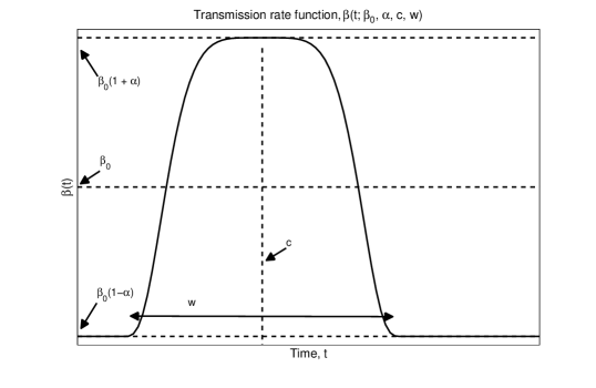
Figure 1: The transmission rate function $\beta(t;\beta_{0},\alpha,c,w)$. The transmission function is chosen to be a smooth, five times differentiable, bump function ranging between $\beta_{0}(1+\alpha)$ at the peak of flu transmission and $\beta_{0}(1-\alpha)$ at the low point. This is done to account for seasonality in our model. The parameters $c$ and $w$ control the center (peak of elevated flu transmission) and width (duration of elevated flu transmission).

Prior distribution estimation

We start by specifying a distribution of model parameterizations that we will consider before any observations from the 2013–2014 season are available. This prior distribution specifies what we think is possible to observe in the new influenza season. Therefore, it is based on the previously observed ILI data and is broad enough to assign a high likelihood to any of the past influenza seasons. Though our method of specifying a prior is reasonable enough to meet this criterion, it does not rely on more rigorous approaches, this will be left to future work.

Let us assume that we have ILI observations from $M$ different influenza seasons. The observations for each season are made at regular intervals, $\Delta t=1\textrm{ week}$, from the end of epidemiological week 32 to the end of epidemiological week 20 of the following year. With the seasons indexed by $i$ we denote these data by

$$d^{i}_{1:K}=(d^{i}_{\Delta t},d^{i}_{2\Delta t},\dots,d^{i}_{K\Delta t})^{T},$$ (2.3)

with $K$ being the number of weeks in each season and $i=1,2,\dots,M$.

A solution of our model is determined by the parameterization vector

$$\mathbf{p}=(S_{0},E_{0},I_{0},\beta_{0},\alpha,c,w,\theta,\gamma)^{T},$$ (2.4)

and each choice of $\mathbf{p}$ yields a discretely sampled solution vector

$$\Psi_{1:K}=(\psi^{T}_{\Delta t},\psi^{T}_{2\Delta t},\dots,\psi^{T}_{K\Delta t},\mathbf{p}^{T})^{T}.$$ (2.5)

The state of our $S^{\nu}\!EIR$ model is denoted by

$$\psi_{t}=(S(t),E(t),I(t))^{T}.$$ (2.6)

The link between our epidemiological model and the data is obtained from the infected proportion at the discrete time points. Specifically, it is the model-to-data map defined by

$$M_{\mathbf{p}}[\Psi_{1:K}]=(100\cdot I(\Delta t),100\cdot I(2\Delta t),\dots,100\cdot I(K\Delta t))^{T},$$ (2.7)

with the multiplication changing the proportion into a percentage, which is what ILI is measured in. Our goal now is to determine a prior distribution for $\mathbf{p}$, $\pi_{0}(\mathbf{p})$, so that samples drawn from the prior, make $M_{p}[\Psi_{1:K}]$ close to at least one prior season’s data set, $d^{i}_{1:K}$.

For each season’s data, $i=1,2,\dots,M$, we can determine an allowable $\mathbf{p}^{i}$ by approximately solving the non-linear optimization problem

$$\mathbf{p}^{i}=\operatorname*{arg\,min}_{\mathbf{p}}\|d^{i}_{1:K}-M_{\mathbf{p}}[\Psi_{1:K}]\|^{2},$$ (2.8)

where $\|\cdot\|$ denotes the root sum of squares discrepancy over the discrete time points. The approximate solution to (2.8) is reached by applying a stochastic optimization algorithm [23, 24] and this process is repeated $L$ times for each season. Variation in these optimal $\mathbf{p}$ for a single season are considered to represent variation that we should allow in the prior distribution of our model. This process then yields $M\cdot L$ approximate solutions $\mathbf{p}^{i}_{l}$, which are then treated as samples from a prior distribution for the model’s parameterization.

A log-normal distribution, fit to these samples, is chosen for $\pi_{0}(\mathbf{p})$. We have chosen a log-normal distribution for $\pi_{0}(\mathbf{p})$ since physically all terms in $\mathbf{p}$ must be positive and the relation of the log-normal to a Gaussian distribution makes it a convenient choice when implementing our ensemble Kalman filtering method.

Data assimilation

An iterative data assimilation process is implemented to continually adjust the parameters and initial state of the seasonal $S^{\nu}\!EIR$ model, which incorporates new ILI and Wikipedia observations. The model can then be propagated through the end of flu season to create an informed forecast. Data assimilation has been successful in a diverse array of fields, from meteorology [32, 20] to economics [16] but has only recently begun to be applied to disease spread [31, 36, 51, 48, 50, 55, 49, 54].

We use an ensemble Kalman smoother (enKS) [20, 21], with propagation always performed from the start of the influenza season, to assimilate the ILI/Wikipedia data into the transmission model. Our implementation of the enKS directly adjusts only the parameterization of our system. However, the adjustment is determined using information about the model’s dynamics throughout the season.

For a more precise description of the ensemble Kalman smoother implemented for this work we refer the reader to [20]. The main idea is to view the time series of our epidemiological model together with its parameters and the ILI/Wikipedia data as a large Gaussian random vector. We can then use standard formulas to condition our $S^{\nu}\!EIR$ time series and parameters on the ILI/Wikipedia observations. Draws from this conditional Gaussian give an updated parameterization of the system from which we can re-propagate to form an updated forecast.

The enKS is similar to a standard ensemble Kalman filter except that instead of just using the most recent data to inform the forecast it uses a number of the most recent observations. The three most current observations, including Wikipedia observations, are used to inform our forecasts. The advantages of using the enKS is that more of the current trends/dynamics of the observations are used in each assimilation step. This helps in estimating the underlying parameterizations of the system by propagating the observation’s information backward into the model ensemble’s history [20, 21].

For each week in the simulation, we receive the ILI data and a Wikipedia estimate of the ILI data. These data become available at regular time intervals of $\Delta t=1\textrm{ week}$ and we denote the data corresponding to the first $K$ weeks by $d_{1:K}$ as in (2.3). Note that now the index $K$ corresponds to the most current week instead of the last week in the season. During the data assimilation step, $d_{1:K}$ is compared with simulations of our $S^{\nu}\!EIR$ model and its parameterization, sampled at weekly intervals, denoted by $\Psi_{1:K}$ as in (2.5) above.

The link between our epidemiological model and the data is again obtained from the simulated infected proportion at the time the most recent data are collected, $K\Delta t$. This is similar to (2.7) except that we only use the infected proportions corresponding to recent data. Specifically, the model-to-data map is

$$M[\Psi_{1:K}]=(100\cdot I((K-2)\Delta t),100\cdot I((K-1)\Delta t),100\cdot I(K\Delta t))^{T}.$$ (2.9)

Using this model-to-data map implies that we are only attempting to model and forecast the dynamics of ILI as opposed to the actual proportion of the U.S. population infected with influenza. The last three sampled values of the infected proportion are used, corresponding to the Wikipedia estimated ILI, the most current ILI, and the previous week’s ILI observations.

In the ensemble Kalman filtering framework, the simulation and data, $(\Psi^{T}_{1:K},d^{T}_{(K-2):K})^{T}$, are assumed to be jointly Gaussian distributed. Therefore, the conditional random vector $\Psi_{1:K}|d_{(K-2):K}$ is also Gaussian, which we can sample from. We only sample the marginal distribution, which is also Gaussian, of our $S^{\nu}\!EIR$ parameterization, $\mathbf{p}|d_{(K-2):K}$. Samples of $\mathbf{p}|d_{(K-2):K}$ are then used to re-propagate our $S^{\nu}\!EIR$ model from an adjusted initial state to form an updated forecast. When new data are collected on the $(K+1)$^th week, the process is repeated.

The remaining details of the enKS implementation deal with the choice of the mean and covariance structure of the joint Gaussian distribution for $(\Psi^{T}_{1:K},d^{T}_{(K-2):K})^{T}$. Our implementation followed Evensen’s explanation [20]. In short, the mean is determined by sampling our $S^{\nu}\!EIR$ model at different parameterizations, while the covariance structure is determined by assumptions on the observational error for ILI, the Wikipedia estimate, and our epidemiological model.

Evaluating forecast accuracy

To evaluate the accuracy of a forecast, we compare the distribution determined by the ensemble with the actual observed disease data. We can, of course, only perform this evaluation retrospectively since we require data to evaluate our forecasts against. Since the enKS method assumes that the forecast distributions are Gaussian, we can evaluate the forecast’s precision by scaling the distance of our forecast mean from the observation using the ensemble covariance. Such a distance has been widely used in statistics and is commonly referred to as the Mahalanobis distance (M-distance) [35]. The M-distance gives a description of the quality of the forecast that accounts for both precision in the mean prediction and precision in the dispersion about the mean. Other methods of evaluating forecast accuracy such as the root mean square error only consider how close the mean of the forecast is to the observations. Thus, a distribution with a great deal of uncertainty, or dispersion, can have a small root mean square error compared to observations.

A forecast is made up of an analysis ensemble of parameterizations $\{\mathbf{p}^{i}_{K}\}_{i=1}^{N}$, $K$ is the index corresponding to the most recently assimilated observation and $N$ is the size of the ensemble. Each $\mathbf{p}^{i}_{K}$ is drawn from a Gaussian distribution conditioned on the most recent observations as described above. We can form a forecast of ILI data for the entire season by propagating the $\mathbf{p}^{i}_{K}$ through our $S^{\nu}\!EIR$ model. We will denote the discretely sampled time series of these realizations by $\psi^{i}_{K}$. The M-distance will then be evaluated using the ensemble of forecast observations, $\{M_{f}[\psi^{i}_{K}]\}_{i=1}^{N}$, corresponding to the infected proportion time series, after the time index $K$, with each $\psi^{i}_{K}$ scaled to a percentage.

The M-distance is then calculated from the $M_{f}[\psi^{i}_{K}]$ using their sample mean and covariance denoted $\mu_{\textrm{obs}}$ and $C_{\textrm{obs}}$, respectively. Letting $\tilde{d}_{K}$ correspond to un-assimilated observations (i.e. observations with time indices greater than $K$) the M-distance we evaluate is

$$\rho(\tilde{d}_{K},\{M_{f}[\psi^{i}_{K}]\})=\sqrt{(\tilde{d}_{K}-\mu_{\textrm{obs}})^{T}C^{-1}_{\textrm{obs}}(\tilde{d}_{K}-\mu_{\textrm{obs}})}.$$ (2.10)

In order to judge the quality of our forecasting methods and ultimately to justify the complexity of our data assimilation procedure, we generate a simplistic straw man model for comparison. We first collect all historical time series of disease outbreaks and then determine a correspondence time between each of the time points for each of the outbreak data sets. This gives a common time frame for each of the historical data sets. Then, at each of these common time points, the average and standard deviation of the historical observations can be computed. Thus, the straw man forecast consists of a normal distribution at each corresponding time point in the forecast with an averaged mean and standard deviation. We can then evaluate the straw man’s accuracy using the metric given in equation (2.10). Given the simple construction of the straw man forecast, this provides a good baseline to necessarily beat, in terms of smaller M-distance, for any compartmental data assimilation-derived forecast.

Besides using a strictly quantitative measure of forecast accuracy, we also suggest computing more qualitative measures of accuracy. With the ensemble forecast, the samples $\psi^{i}_{K}$ can be used to estimate quantiles of the forecast distribution such as the standard 5-number summary of the distribution given by the 5%, 25%, 50%, 75%, and 95% quantiles for the seasonal $S^{\nu}EIR$ realizations. Moreover, if we are interested in the forecast of some other quantity of interest derived from the time series of observations, such as the epidemic’s peak time, peak level, duration, or start time, we may also derive 5-number summaries for these quantities by computing the appropriate quantity of interest. Analyzing where the actual observations fall compared to the 5-number summary provides a qualitative way to understand the accuracy of the forecast.

3 Results

We present the results of our prior estimation techniques and our evaluation of forecast accuracy for the 2013–2014 influenza season. Again, for the reasons mentioned above, the influenza season is defined to be between the 32^nd and 20^th epidemiological weeks for successive years. Our forecasts are only valid during this time period.

Prior forecast

Historical ILI data from the 2003–2004 U.S. influenza season through the 2012–2013 influenza season was used to generate our prior distribution of the seasonal $S^{\nu}\!EIR$ model’s parameterization. This was done following the methods described above. An example fit using a stochastic optimization algorithm to find 10 approximate solutions to (2.8) for the 2006–2007 ILI data is shown in Figure 2. Two things can be noticed from this fit of our epidemiological model. First, there is often a small early peak in the ILI data before the primary peak and our model does a poor job of capturing this. Second, the ILI data usually remains elevated longer than our model’s realizations can support. Both of these areas point to systematic divergence of the model from data.

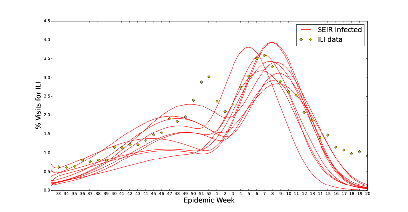
Figure 2: Seasonal $S^{\nu}\!EIR$ fit to 2006–2007 U.S. ILI data. Ten seasonal heterogeneous $S^{\nu}\!EIR$ model parameterizations for the U.S. ILI 2006–2007 data. These are approximate solutions to (2.8). For each of the influenza seasons, from 2003–2004 through 2012–2013, fits similar to the above were generated. These parameterizations formed the basis for our prior, $\pi_{0}(\mathbf{p})$. This is a good example of the seasonal $S^{\nu}\!EIR$ model’s two areas of systematic divergence. In the weeks 50–1 there is a first peak that the model does not catch. During the tail weeks 15–20 our $S^{\nu}\!EIR$ model tapers too quickly.

From the joint prior, $\pi_{0}(\mathbf{p})$, we can examine samples from the marginal priors to examine our method’s forecast for traits of the average influenza season. In Figure 3 we show histograms of samples from a few of these marginal priors. We see that our methods have determined that the average base time of transmission is 2–5 days, the average incubation time is 3–7 days, and the average recovery time is 6–8 days. This automatically lets us know that the recovery rate is tightly specified by our prior whereas the base transmission and incubation rates are not. Since our $S^{\nu}\!EIR$ model includes a variable transmission rate, we also include the marginals for the week of peak transmissibility, $c$, and the duration the transmission rate is elevated, $w$. For our prior, the duration is centered over 14–20 weeks, while the center is between simulation week 20 and 30, corresponding to the epidemiological weeks 52 and 10 of 2013 and 2014, respectively.

$\begin{array}[]{cc}\includegraphics[scale={0.2}]{figure4.pdf}&\includegraphics[scale={0.2}]{figure5.pdf}\\ \includegraphics[scale={0.2}]{figure6.pdf}&\includegraphics[scale={0.2}]{figure7.pdf}\\ \includegraphics[scale={0.2}]{figure8.pdf}&\end{array}$

Figure 3: Histograms of model parameter prior distributions. All histograms were generated from 300 samples of $\pi_{0}(\mathbf{p})$. (TOP LEFT) Histogram of the marginal distribution for the average transmission time, measured in days. The rate parameter, $\beta_{0}$, is then the inverse of this average time. (TOP RIGHT) marginal distribution for the average incubation time, measured in days. The rate parameter in our $S^{\nu}\!EIR$ model, $\theta$, is then the inverse of this average time. We see that this distribution is concentrated over 3–6 days and skewed toward longer incubation times. (MIDDLE LEFT) Histogram of the marginal distribution for the average recovery time, measured in days. The rate parameter in our $S^{\nu}\!EIR$ model, $\gamma$, is the inverse of this average time. We see that this distribution is concentrated over 6–7 days and skewed toward longer incubation times. The prior distribution for $\gamma$ is more concentrated than the distributions for $\theta$ and $\beta_{0}$ which means that the ILI data determine this parameter more exactly. (MIDDLE RIGHT) Histogram of the marginal distribution for the peak of the transmissibility function, $\beta(t;\beta_{0},\alpha,c,w)$. The parameter $c$ here is represented in weeks since the beginning of simulation. Thus, a value $c=16$ corresponds to the peak transmissibility during the 48^th epidemiological week. We see that this distribution is concentrated over 20–30 weeks into the simulation and skewed toward late in the simulation. (BOTTOM LEFT) Histogram of the marginal distribution for the duration of heightened transmissibility. The parameter $w$ is represented in weeks. A value $w=14$ corresponds to 16 weeks of elevated transmission. We see that this distribution is concentrated over 14–20 weeks and skewed toward longer periods of elevated transmission.

Sampling 300 parameterization from the log-normal prior $\pi_{0}(\mathbf{p})$ leads to the prior forecast for the 2013–2014 influenza season shown in Figure 4. One can notice that our prior forecast allows for a wide range of peak times and sizes. In general, the earlier the peak the smaller its forecast height. It is also apparent that our forecast tapers off quickly after the peak occurs.

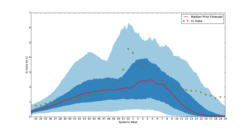
Figure 4: U.S. ILI prior forecast for 2013–2014 flu season. This figure shows the prior forecast along with the 2013–2014 ILI data. Note the potential for an early and late peaking influenza season. The red line represents the median forecast from 300 samples of the prior. The dark blue and light blue regions represent the 50% and 90% credible regions centered around this median, respectively. Credible intervals were also generated from 300 samples of the prior.

Forecast analysis

In Figure 5 we show the results of our forecasting process for two different weeks during the 2013–2014 influenza season. Note, the performance of the seasonal $S^{\nu}\!EIR$ model is drastically reduced once the peak of the influenza season has past. However, before the peak, the model forecasts a range of possible influenza scenarios that include the 2013–2014 season. In Figure 6, we show the forecast resulting from the straw man approach for the 2013–2014 influenza season. In this section, we analyze both of these forecast’s performance using the measures described above.

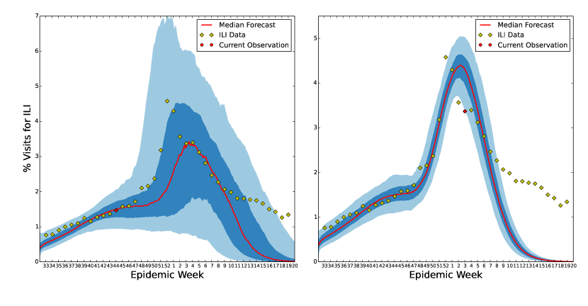
Figure 5: U.S. ILI forecast for the 2013–2014 flu season made during the 43^rd (left) and 2^nd (right) epidemiological weeks. In each plot the dark blue region represents the region centered about the median in which 50% of forecasts fall, the light blue region represents where 90% of forecasts fall, and the red line represents the median forecast. The diamonds represent the 2013–2014 ILI data with the current data point marked by a red circle.

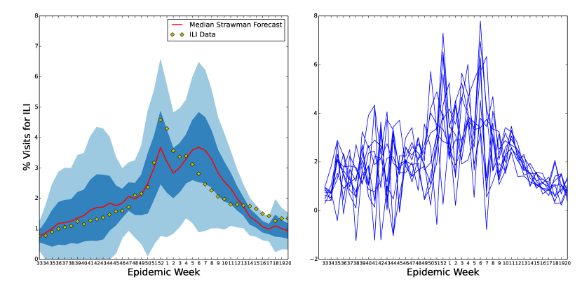
Figure 6: U.S. ILI Straw Man forecast. This figure shows the results of our straw man prediction based on averaging past flu seasons. Since this forecast of the 2013–2014 influenza season was made using only the statistics of the sample mean and sample standard deviation from previous season’s ILI observations it’s credible intervals (left) do a good job of containing the current influenza season. However, this is at the cost of having large credible intervals representing a large amount of uncertainty in the forecast. Also, this forecast does not include any causal model of influenza spread. There is, therefore, no correlation between the forecast at successive time points. This is seen when sampling time series from this forecast (right).

Quantitative Accuracy

In Figure 7 we show the successive M-distances computed for our forecast and for 300 samples from the straw man forecast. We notice that up until the peak of the 2013–2014 influenza season, the data-assimilative forecasting scheme has a noticeably smaller M-distance than that of the straw man forecast. However, after the peak of the influenza season, during week 52 for 2013–2014, the straw man shows considerably smaller M-distance. This is due to the seasonal $S^{\nu}\!EIR$’s inability to taper off slowly from the peak of the flu season. After the peak, our model has exhausted its susceptible proportion of the population, and the infected proportion rapidly goes to zero. A possible point of confusion in this analysis is the sharp drop off of the M-distance as the end of our forecast horizon is approached. This is due to the decreased dimension of the data being forecasted. During week 17, the forecasts only need to predict the ILI data for 3 more weeks and distances in this 3-dimensional space grow much slower as a function of week-by-week error.

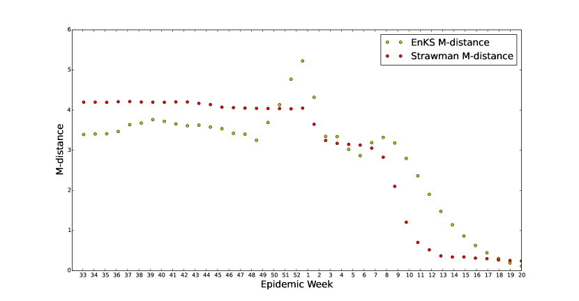
Figure 7: $S^{\nu}\!EIR$ with enKS vs. Straw Man forecast for the 2013–2014 U.S. ILI data. The M-distance between U.S. 2013–2014 ILI data and the two forecasts is plotted. The M-distance between the forecast and ILI data is calculated for each epidemiological week until the end of the influenza season. So the M-distances at week 36 uses the forecast observations from week 36 of 2013 to week 20 of 2014 and the ILI data from week 36 of 2013 to week 20 of 2014. The M-distances plotted for the straw man prediction use sample covariances and means calculated from 300 time series draws of the straw man forecast. Due to the lack of causal relations included in the straw man model this measure of accuracy is significantly lower in the early season for the straw man prediction. This figure shows that the data assimilation forecast has a noticeably smaller M-distance, and therefore is quantitatively better, than the straw man model for the early influenza season. Once the influenza season peaks the success of the forecast breaks down due to model error. It is interesting to note that due to the enKS data assimilation our $S^{\nu}\!EIR$ forecast seems to attempt self-correction, i.e. the M-distance is increasing and then decreases.

Qualitative Accuracy

Each week, given the 300 infected time series from the analyzed ensemble, we gain 300 samples of the epidemic peak percent infected, the epidemic start time, the epidemic duration, and the week of the epidemic peak. From these 300 samples of these quantities of interest, we estimate the 5%, 25%, 50%, 75%, and 95% posterior quantiles. The start of the influenza season is defined to be the first week that ILI goes above 2% and remains elevated for at least 3 consecutive weeks. The end of the influenza season, used to calculate the duration, is when ILI goes below the 2% national baseline and remains there. This gives us a convenient weekly summary of our influenza forecast with uncertainty quantified by 95% posterior credible intervals about the median.

A time series plot of the start week credible intervals for our seasonal $S^{\nu}\!EIR$ forecast is shown in Figure 8. A similar plot for the start week credible intervals forecast using the straw man model would show a constant distribution with median start week forecast at the 38^th epidemiological week. We can see for Figure 8 that the high probability region for start week, as forecast by our epidemiological model, is usually 1–2 weeks after the actual 2013–2014 start week. However, the actual start week is contained within the 95% confidence region until a week or two after the peak of flu season. This region is also seen to constrict as ILI and Wikipedia observations are assimilated.

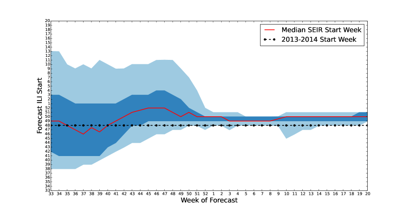
Figure 8: $S^{\nu}\!EIR$ start week quantiles for 2013–2014 U.S. ILI. 50% and 90% credible interval estimates of the influenza season start week are plotted along with the median. Each week, as new ILI data become available the forecast is revised. This causes the uncertainty in our forecast to diminish. However, due to the model’s inability to maintain an elevated ILI level past the peak, we see that late in the flu season, the model adjusts by pushing the start week later into the season. This causes an overestimation of the start week that worsens as the season progresses.

When compared to the forecast start week from the straw man model, our $S^{\nu}\!EIR$ model seems like a favorable tool. The straw man’s forecast does not assimilate current observations and thus its predicted start week is constant. Two things should be mentioned about calculating these credible intervals for the straw man forecast. First, since a sample from the straw man forecast has no week-to-week correlations, the weekly forecasts can vary greatly from week to week. This is a problem when computing the start week for the influenza season since a given straw man sample does not remain above 2% for consecutive weeks. Second, for similar reasons the duration cannot even be defined for one time series sample of the straw man forecast.

4 Discussion

Summary of method

We have outlined an approach to forecasting seasonal influenza that relies on modern ensemble data assimilation methods for updating a prior distribution of a disease transmission model. The method used a dynamic compartmental model of influenza spread that has been used in previous research [46, 53, 30] but is applicable to any compartmental model of disease with a regularly updated public health data source.

We evaluated the accuracy of our forecast using the M-distance, based on the Gaussian likelihood of observations, and the deviation of time series of quantiles for a set of quantities of interest arising from flu dynamics. Both of these methods were used on our data assimilation approach and on a much simpler forecast using estimated normal distributions. The application of these measures of accuracy, combined with our specific approach to data assimilation with a dynamic model of the influenza dynamics allowed us to highlight model inaccuracies that can then be improved in the future.

Though a statistically simple tool, the inclusion of a straw man forecast as a baseline to evaluate our data assimilation scheme’s usefulness is indispensable when evaluating measures of accuracy. Especially for some measure, such as the M-distance, it is difficult to tell whether or not a value implies the forecast performed well without a baseline. We hope that the approach of measuring a forecast against a baseline becomes established practice in future developments of epidemic forecasting.

The differential equation representation of influenza dynamics, modeled proportions of the population as susceptible, exposed/non-infectious, symptomatic/infectious, and recovered/immune/removed. Thus, the model did not allow for any re-infection of influenza, which is thought to be biologically accurate for at least a single strain of flu [3]. We also modeled the effect of heterogeneity in the influenza contact network and seasonal variation in the transmissibility of flu. Our method of data assimilation adjusted the allowable parameterizations and initializations of this model as ILI data became available.

The forecast was made up of actual realizations of our $S^{\nu}\!EIR$ model used. This has the arguable advantage of highlighting observed sections of the ILI data stream that differ drastically from the model’s assumptions. However, since the model state is not adjusted at each ILI data point directly, the forecast with an incorrect model eventually diverges from the data.

To iteratively update the prior distributions of parameterizations and initializations, we used an ensemble Kalman smoother. This was observed to significantly pull the model toward a subset of parameterizations and initializations that agreed well with the data. Since the model seemed to be reasonably adjusted toward observations and retained a significant amount of ensemble variation in the forecast, there is strong evidence that the assimilation scheme works well. The challenge now is to arrive at a model that more accurately represents influenza dynamics perhaps by including considerations made in [3, 18, 17, 52, 5, 34].

Our quantitative measure of forecast accuracy is motivated by the Gaussian likelihood function and has been used, in many instances, to assign a value to the distance from some predicted distribution with a fixed mean and covariance. This is exactly the setting we are in, when we make the Gaussian assumptions inherent in the Kalman filter methods. The application of the M-distance in this instance showed that our model performed better than the simple straw man forecast in the beginning of the season but then systematically diverged from the late season ILI data.

Besides demonstrating the accuracy of our forecast at capturing overall dynamics, we also quantified our forecating method’s ability to accurately estimate quantities of interest relating to the impact of a given influenza season. We showed how the time series of forecast median and posterior credible intervals for the season’s start week, peak week, duration, and peak level changed over time. This measure in particular demonstrated the advantages of having an underlying mechanistic model as compared to the purely statistical normal approximation forecast as used in the straw man forecast.

Future improvements and lessons learned

This work shows the viability of using a data assimilation method to sequentially tune a model of disease dynamics. However, it also highlights the need to use caution when adjusting the model to match data. If balances inherent in the model are not maintained during each adjustment step, it is possible to forecast data accurately with a model that is incorrect (e.g., one that has no single realization that will reproduce the data up to data error). The upside of this approach is that if only the model parameterization and initialization are adjusted, this type of forecasting process allows one to identify the assumptions of the model that diverge from observations. This is an important tool, to advance models to more accurate representations of reality, that could be ignored if data assimilation methods are used to adjust a model’s state and parameterization throughout the forecast.

The method proposed here, which maintain $S^{\nu}\!EIR$ balances during assimilation, are not the only possible methods of maintaining the population balances assumed in a compartmental disease model. More research needs to be done on the best way to adjust a model to observations while maintaining an accurate representation of disease model balances. Moreover, if the goal is to create forecasts for multiple seasons, forecasting from initial conditions will not always be viable. It remains an important open research question as to how far in the past one should optimally start forecasts from. The farther in the past a forecast is made from, the more dynamics of the model and data are assimilated. The downside of this is that considering too much of the models dynamics can impose unnecessary restrictions on the prior, leading to a divergent forecast.

A major concern for our epidemiological model is the systematic divergence from the data at the end of the influenza season. This divergence is evident in the optimal fitting done with our $S^{\nu}\!EIR$ model on historical ILI data. The CDC, in collaboration with World Health Organization and the National Respiratory and Enteric Virus Surveillance System, also releases some data about flu strain circulation during the season [2]. These data show that often there are one or two outbreaks of secondary dominant influenza strains in the late season. We hypothesize that these secondary strains are a primary cause of the heightened tail in the ILI data and we will investigate a multi-strain influenza model [3] in future forecasting work.

References

- [1] National strategy for biosurveillance. Technical report, The White House, jul 2012.
- [2] Overview of influenza surveillance in the United States. Technical report, Centers for Disease Control and Prevention, 2012.
- [3] Jorge A Alfaro-Murillo, Sherry Towers, and Zhilan Feng. A deterministic model for influenza infection with multiple strains and antigenic drift. Journal of biological dynamics, 7(1):199–211, 2013.
- [4] Roy M Anderson and Robert M May. Infectious diseases of humans: Dynamics and control. Oxford University Press, 1991.
- [5] Paolo Bajardi, Chiara Poletto, Jose J Ramasco, Michele Tizzoni, Vittoria Colizza, and Alessandro Vespignani. Human mobility networks, travel restrictions, and the global spread of 2009 h1n1 pandemic. PloS one, 6(1):e16591, 2011.
- [6] Duygu Balcan, Hao Hu, Bruno Goncalves, Paolo Bajardi, Chiara Poletto, Jose J Ramasco, Daniela Paolotti, Nicola Perra, Michele Tizzoni, Wouter V Broeck, et al. Seasonal transmission potential and activity peaks of the new influenza a (h1n1): a monte carlo likelihood analysis based on human mobility. BMC medicine, 7(1):45, 2009.
- [7] Luis Bettencourt and Ruy Ribeiro. Real time bayesian estimation of the epidemic potential of emerging infectious diseases. PLOS One, 3(5), 2008.
- [8] Luís M. A. Bettencourt et al. Towards real time epidemiology: Data assimilation, modeling and anomaly detection of health surveillance data streams. In Daniel Zeng et al., editors, Intelligence and Security Informatics: Biosurveillance. Springer, 2007.
- [9] Carles Bretó, Daihai He, Edward L Ionides, and Aaron A King. Time series analysis via mechanistic models. The Annals of Applied Statistics, pages 319–348, 2009.
- [10] Guthrie S Burkhead and Christopher M Maylahn. State and Local Public Health Surveillance. In Steven M Teutsch and R Elliot Churchill, editors, Principles and Practice of Public Health Surveillance, chapter 12, pages 253–286. Oxford University Press, 2nd edition, 2000.
- [11] B Cazelles and NP Chau. Using the kalman filter and dynamic models to assess the changing hiv/aids epidemic. Mathematical biosciences, 140(2):131–154, 1997.
- [12] CDC. Announcement of requirements and registration for the predict the influenza season challenge, 2013. [Online; accessed 15-September-2014].
- [13] Prithwish Chakraborty, Pejman Khadivi, Bryan Lewis, Aravindan Mahendiran, Jiangzhuo Chen, Patrick Butler, Elaine O Nsoesie, Sumiko R Mekaru, John S Brownstein, Madhav Marathe, et al. Forecasting a moving target: Ensemble models for ili case count predictions. In Proceedings of the 2014 SIAM International Conference on Data Mining, pages 262–270. SIAM, 2014.
- [14] Jean-Paul Chretien, Dylan George, Jeffrey Shaman, Rohit A Chitale, and F Ellis McKenzie. Influenza forecasting in human populations: A scoping review. PloS one, 9(4):e94130, 2014.
- [15] Loren Cobb, Ashok Krishnamurthy, Jan Mandel, and Jonathan D Beezley. Bayesian tracking of emerging epidemics using ensemble optimal statistical interpolation. Spatial and spatio-temporal epidemiology, 2014.
- [16] Drew Creal. A survey of sequential Monte Carlo methods for economics and finance. Econometric Reviews, 31(3), 2012.
- [17] S. Y. Del Valle et al. Mixing patterns between age groups in social networks. Social Networks, 29(4), October 2007.
- [18] Sara Y. Del Valle et al. Modeling the impact of behavior changes on the spread of pandemic influenza. In Modeling the interplay between human behavior and the spread of infectious diseases. Springer, 2013.
- [19] Christl A Donnelly, Azra C Ghani, Gabriel M Leung, Anthony J Hedley, Christophe Fraser, Steven Riley, Laith J Abu-Raddad, Lai-Ming Ho, Thuan-Quoc Thach, Patsy Chau, King-Pan Chan, Tai-Hing Lam, Lai-Yin Tse, Thomas Tsang, Shao-Haei Liu, James HB Kong, Edith MC Lau, Neil M Ferguson, and Roy M Anderson. Epidemiological determinants of spread of causal agent of severe acute respiratory syndrome in hong kong. The Lancet, 361(9371):1761–1766, May 2003.
- [20] Geir Evensen. Data assimilation: The ensemble Kalman filter. Springer, 2009.
- [21] Geir Evensen and Peter Jan Van Leeuwen. An ensemble kalman smoother for nonlinear dynamics. Monthly Weather Review, 128(6):1852–1867, 2000.
- [22] Christophe Fraser, Christl A. Donnelly, Simon Cauchemez, William P. Hanage, Maria D. Van Kerkhove, T. Déirdre Hollingsworth, Jamie Griffin, Rebecca F. Baggaley, Helen E. Jenkins, Emily J. Lyons, Thibaut Jombart, Wes R. Hinsley, Nicholas C. Grassly, Francois Balloux, Azra C. Ghani, Neil M. Ferguson, Andrew Rambaut, Oliver G. Pybus, Hugo Lopez-Gatell, Celia M. Alpuche-Aranda, Ietza Bojorquez Chapela, Ethel Palacios Zavala, Dulce Ma Espejo Guevara, Francesco Checchi, Erika Garcia, Stephane Hugonnet, and Cathy Roth. Pandemic potential of a strain of influenza a (H1N1): early findings. Science, 324(5934):1557–1561, June 2009.
- [23] Zong Woo Geem, Joong Hoon Kim, and G V Loganathan. A New Heuristic Optimization Algorithm: Harmony Search. Simulation, 76(2):60–68, feb 2001.
- [24] ZW Geem. Improved harmony search from ensemble of music players. In Knowledge-based intelligent information and engineering systems. Springer, jan 2006.
- [25] Nicholas Generous, Geoffrey Fairchild, Alina Deshpande, Sara Y. Del Valle, and Reid Priedhorsky. Global disease monitoring and forecasting with wikipedia. PLOS Computational Biology, To Appear, 2014.
- [26] Timothy C. Germann et al. Mitigation strategies for pandemic influenza in the United States. PNAS, 103(15), April 2006.
- [27] Jeremy Ginsberg et al. Detecting influenza epidemics using search engine query data. Nature, 457(7232), November 2008.
- [28] Herbert W. Hethcote. The mathematics of infectious diseases. SIAM Review, 42(4), January 2000.
- [29] R.S. Hopkins, A. Kite-Powell, K. Goodin, and J.J. Hamilton. The ratio of emergency department visits for ili to seroprevalence of 2009 pandemic influenza a (h1n1) virus infection, florida, 2009. PLOS Currents Outbreaks, June 2014.
- [30] James M Hyman and Tara LaForce. Modeling the spread of influenza among cities. Bioterrorism: Mathematical modeling applications in homeland security, 28:211, 2003.
- [31] C. Jégat et al. Early detection and assessment of epidemics by particle filtering. In Geostatistics for environmental applications. Springer, January 2008.
- [32] Eugenia Kalnay. Atmospheric modeling, data assimilation, and predictability. Cambridge University Press, 2003.
- [33] V. Lampos and N. Cristianini. Tracking the flu pandemic by monitoring the social web. In Proc. Workshop on Cognitive Information Processing (CIP). IEEE, 2010.
- [34] Bruce Y. Lee et al. A computer simulation of vaccine prioritization, allocation, and rationing during the 2009 H1N1 influenza pandemic. Vaccine, 28(31), July 2010.
- [35] Prasanta Chandra Mahalanobis. On the generalized distance in statistics. Proceedings of the National Institute of Sciences (Calcutta), 2:49–55, 1936.
- [36] Jan Mandel et al. Data driven computing by the morphing fast Fourier transform ensemble Kalman filter in epidemic spread simulations. Procedia Computer Science, 1(1), May 2010.
- [37] David J McIver and John S Brownstein. Wikipedia usage estimates prevalence of influenza-like illness in the united states in near real-time. PLoS computational biology, 10(4):e1003581, 2014.
- [38] Elaine Nsoesie, Madhav Mararthe, and John Brownstein. Forecasting peaks of seasonal influenza epidemics. PLoS currents, 5, 2013.
- [39] Elaine O Nsoesie, Richard Beckman, Madhav Marathe, and Bryan Lewis. Prediction of an epidemic curve: A supervised classification approach. Statistical communications in infectious diseases, 3(1), 2011.
- [40] Elaine O Nsoesie, Richard J Beckman, Sara Shashaani, Kalyani S Nagaraj, and Madhav V Marathe. A simulation optimization approach to epidemic forecasting. PloS one, 8(6):e67164, 2013.
- [41] Elaine O Nsoesie, John S Brownstein, Naren Ramakrishnan, and Madhav V Marathe. A systematic review of studies on forecasting the dynamics of influenza outbreaks. Influenza and other respiratory viruses, 8(3):309–316, 2014.
- [42] Elaine O Nsoesie, Scotland C Leman, and Madhav V Marathe. A dirichlet process model for classifying and forecasting epidemic curves. BMC infectious diseases, 14(1):12, 2014.
- [43] Jimmy Boon Som Ong, I Mark, Cheng Chen, Alex R Cook, Huey Chyi Lee, Vernon J Lee, Raymond Tzer Pin Lin, Paul Ananth Tambyah, and Lee Gan Goh. Real-time epidemic monitoring and forecasting of h1n1-2009 using influenza-like illness from general practice and family doctor clinics in singapore. PloS one, 5(4):e10036, 2010.
- [44] Reid Priedhorsky, Aron Culotta, and Sara Y. Del Valle. Inferring the origin locations of tweets with quantitative confidence. In Proc. Computer Supported Cooperative Work (CSCW), 2014. To appear.
- [45] C.J. Rhodes and T.D. Hollingsworth. Variational data assimilation with epidemic models. Journal of Theoretical Biology, 258(4), June 2009.
- [46] Ronald Ross. The prevention of malaria. Dutton, 1910.
- [47] Cosmin Safta, Jaideep Ray, Sophia Lefantzi, David Crary, Khachik Sargsyan, and Karen Cheng. Real-time characterization of partially observed epidemics using surrogate models. Technical report, Sandia National Laboratories, 2011.
- [48] Jeffrey Shaman and Alicia Karspeck. Forecasting seasonal outbreaks of influenza. PNAS, 109(50), December 2012.
- [49] Jeffrey Shaman, Alicia Karspeck, Wan Yang, James Tamerius, and Marc Lipsitch. Real-time influenza forecasts during the 2012–2013 season. Nature communications, 4, 2013.
- [50] Daniel M Sheinson, Jarad Niemi, and Wendy Meiring. Comparison of the performance of particle filter algorithms applied to tracking of a disease epidemic. Mathematical biosciences, 2014.
- [51] Alex Skvortsov and Branko Ristic. Monitoring and prediction of an epidemic outbreak using syndromic observations. Mathematical Biosciences, 240(1), November 2012.
- [52] Phillip Stroud et al. Spatial dynamics of pandemic influenza in a massive artificial society. Artificial Societies and Social Simulation, 10(4), 2007.
- [53] Phillip D. Stroud et al. Semi-empirical power-law scaling of new infection rate to model epidemic dynamics with inhomogeneous mixing. Mathematical Biosciences, 203(2), October 2006.
- [54] Wan Yang, Alicia Karspeck, and Jeffrey Shaman. Comparison of filtering methods for the modeling and retrospective forecasting of influenza epidemics. PLoS computational biology, 10(4):e1003583, 2014.
- [55] Wan Yang and Jeffrey Shaman. A simple modification for improving inference of non-linear dynamical systems. arXiv preprint arXiv:1403.6804, 2014.