Direct numerical simulation of turbulent channel flow up to $Re_{\tau}\approx$ 5200

Abstract

A direct numerical simulation of incompressible channel flow at $Re_{\tau}=5186$ has been performed, and the flow exhibits a number of the characteristics of high Reynolds number wall-bounded turbulent flows. For example, a region where the mean velocity has a logarithmic variation is observed, with von Kármán constant $\kappa=0.384\pm 0.004$. There is also a logarithmic dependence of the variance of the spanwise velocity component, though not the streamwise component. A distinct separation of scales exists between the large outer-layer structures and small inner-layer structures. At intermediate distances from the wall, the one-dimensional spectrum of the streamwise velocity fluctuation in both the streamwise and spanwise directions exhibits $k^{-1}$ dependence over a short range in $k$. Further, consistent with previous experimental observations, when these spectra are multiplied by $k$ (premultiplied spectra), they have a bi-modal structure with local peaks located at wavenumbers on either side of the $k^{-1}$ range.

1 Introduction

Recently, relatively “high” Reynolds number wall-bounded turbulence has been investigated with the help of innovations in measurement technologies (Nagib et al., 2004; Kunkel & Marusic, 2006; Westerweel et al., 2013; Bailey et al., 2014) and computation (Lee et al., 2013; Borrell et al., 2013; El Khoury et al., 2013). Because of the simplicity in geometry and boundary conditions, pressure-driven turbulent flow between parallel walls (channel flow) is an excellent vehicle for the study of wall-bounded turbulence via direct numerical simulation (DNS). Since Kim et al. (1987) showed agreement between DNS and experiments in channel flow in 1987, DNS of channel flow has been used to study wall-bounded turbulence at ever higher Reynolds number, as advances in computing power allowed. For example, channel flow DNS were performed at $Re_{\tau}=590$ (Moser et al., 1999), $Re_{\tau}=950$ (Del Álamo et al., 2004), and $Re_{\tau}=2000$ (Hoyas & Jiménez, 2006). More recently, simulations with $Re_{\tau}\approx 4000$ were performed separately by Lozano-Durán & Jiménez (2014) in a relatively small domain size and by Bernardini et al. (2014). Also, to investigate the differences between channel flow turbulence and boundary layer turbulence, a simulation at $Re_{\tau}=2000$ of a zero pressure gradient boundary layer was performed by Sillero et al. (2013).

The idealized channel flow that is so straight-forward to simulate is more difficult to realize experimentally because of the need for side walls. Measurements of channel flow are not as numerous as for other wall bounded turbulent flows, but a number of studies have been conducted over the years (Comte-Bellot, 1963; Dean & Bradshaw, 1976; Johansson & Alfredsson, 1982; Wei & Willmarth, 1989; Zanoun et al., 2003, 2009; Monty & Chong, 2009). Of particular interest here will be the channel measurements made by Schultz & Flack (2013) at Reynolds number up to $Re_{\tau}=6000$, because they bracket the Reynolds number simulated here.

Turbulent flows with $Re_{\tau}$ on the order of $10^{3}$ and greater are of interest because this is the range of Reynolds numbers relevant to industrial applications (Smits & Marusic, 2013). Further, it is in this range that characteristics of wall-bounded turbulence associated with high Reynolds number are first manifested (Marusic et al., 2010b), and so studies of these phenomena must necessarily be conducted at these Reynolds numbers. The best-known feature of high-Reynolds number wall-bounded turbulence is the logarithmic law in the mean velocity, which has been known since the 1930’s (Millikan, 1938). The von Kármán constant $\kappa$ that appears in the log-law, is also an important parameter for calibrating turbulence models (Durbin & Pettersson Reif, 2010; Marusic et al., 2010b; Smits et al., 2011; Spalart & Allmaras, 1992). It was considered universal in the past, but Nagib & Chauhan (2008) showed that $\kappa$ can be different in different flow geometries. Further, Jiménez & Moser (2007) found that channel flows with $Re_{\tau}$ up to 2000, do not exhibit a region where the mean velocity profile strictly follows a logarithmic law, and showed that a finite Reynolds number correction like that introduced by Afzal (1976) was more consistent with data in this Reynolds number range. Similarly, Mizuno & Jiménez (2011) used a different finite Reynolds number correction to represent the overlap region in boundary layers, channels and pipes.

For turbulent intensities, Townsend (1976) predicted that, in high Reynolds number flows, there are regions where the variance of the streamwise and spanwise velocity components decrease logarithmically with distance from the wall. This has been observed experimentally for streamwise (Kunkel & Marusic, 2006; Winkel et al., 2012; Hultmark et al., 2012; Hutchins et al., 2012; Marusic et al., 2013) and spanwise components (Fernholz & Finley, 1996; Morrison et al., 2004), but has only been observed in the spanwise component in DNS (Hoyas & Jiménez, 2008; Sillero et al., 2013). Further, the peak of the streamwise velocity variance has a weak Reynolds number dependence when it is scaled by friction velocity, $u_{\tau}$ (DeGraaff & Eaton, 2000; Hoyas & Jiménez, 2006).

There has also been recent interest in the role of large scale motions (LSM) in high Reynolds number wall-bounded turbulent flow (Kim & Adrian, 1999; Hutchins & Marusic, 2007; Wu et al., 2012). According to the scaling analysis of Perry et al. (1986) there is a region where the one-dimensional spectral energy density has a $k_{x}^{-1}$ dependence. This has been supported by experimental evidence (Nickels et al., 2005, 2007), but not numerical simulations.

In summary, there are many characteristics of high-Reynolds-number wall-bounded turbulence that have been suggested by theoretical arguments and corroborated experimentally, but which have not been observed in direct numerical simulations, presumably due to the limited Reynolds numbers of the simulations. This is unfortunate because such simulations could provide detailed information about these high Reynolds number phenomena that would not otherwise be available. The direct numerical simulation reported here was undertaken to address this issue, by simulating a channel flow at sufficiently high Reynolds number and with sufficiently large spatial domain to exhibit characteristics of high-Reynolds number turbulence like those discussed above. The simulation was performed for $Re_{\tau}\approx 5200$ with the same domain size used by Hoyas & Jiménez (2006) in their $Re_{\tau}=2000$ simulation.

This paper is organized as follows. First, the simulation methods and parameters are described in §2, along with other simulations and experiments used for comparison. Results of the simulation that arise due to the relatively high Reynolds number of the simulation are presented in §3. Finally, conclusions are offered in §4.

2 Simulation Details

In the discussion to follow, the streamwise, wall-normal and spanwise velocities will be denoted $u$, $v$ and $w$ respectively with the mean velocity indicated by a capital letter, and fluctuations by a prime. Furthermore, $\langle\cdot\rangle$ indicates the expected value or average. Thus $U=\langle u\rangle$ and $u=U+u^{\prime}$.

The simulations reported here are DNS of incompressible turbulent flow between two parallel planes. Periodic boundary conditions are applied in the streamwise ($x$) and spanwise ($z$) directions, and no-slip/no-penetration boundary conditions are applied at the wall. The computational domain sizes are $L_{x}=8\pi\delta$ and $L_{z}=3\pi\delta$, where $\delta$ is the channel half-width, so the domain size in the wall-normal ($y$) direction is $2\delta$. The flow is driven by a uniform pressure gradient, which varies in time to ensure that the mass flux through the channel remains constant.

A Fourier-Galerkin method is used in the streamwise and spanwise directions, while the wall-normal direction is represented using a B-spline collocation method (Kwok et al., 2001; Botella & Shariff, 2003). The Navier-Stokes equations are solved using the method of Kim et al. (1987), in which equations for the wall-normal vorticity and the Laplacian of the wall-normal velocity are time-advanced. This formulation has the advantage of satisfying the continuity constraint exactly while eliminating the pressure. A low-storage implicit-explicit scheme (Spalart et al., 1991) based on third-order Runge-Kutta for the non-linear terms and Crank-Nicolson for the viscous terms is used to advance in time. The time step is adjusted to maintain an approximately constant CFL number of one. A new highly optimized code was developed to solve the Navier-Stokes equations using these methods on advanced peta-scale computer architectures. For more details about the code, the numerical methods, and how the simulations were run, see Lee et al. (2013, 2014).

The simulations performed here were conducted with resolution comparable to that used in previous high Reynolds number channel flow simulations, when measured in wall units. Normalization in wall units, that is, with kinematic viscosity $\nu$ and friction velocity $u_{\tau}$, is indicated with a superscript “+”. The friction velocity is $u_{\tau}=\sqrt{\tau_{w}/\rho}$, where $\tau_{w}$ is the mean wall shear stress. For the highest Reynolds number simulation reported here, which is designated LM5200, $N_{x}=10240$ and $N_{z}=7680$ Fourier modes were used to represent the streamwise and spanwise direction, which results in an effective resolution $\Delta x^{+}=L_{x}^{+}/N_{x}=12.7$ and $\Delta z^{+}=L_{z}^{+}/N_{z}=6.4$. In the wall normal direction, the seventh order B-splines are defined on a set of $1530=N_{y}-6$ knot points ($N_{y}$ is the number of B-spline basis functions), which are distributed uniformly in a mapped coordinate $\xi$ that is related to the wall-normal coordinate $y$ through

$$\frac{y}{\delta}=\frac{\sin\left(\eta\xi\pi/2\right)}{\sin\left(\eta\pi/2\right)},\quad-1\leq\xi\leq 1$$

The single parameter $\eta$ in this mapping controls how strongly the knot points are clustered near the wall, with the strongest clustering occurring when $\eta=1$. In LM5200, $\eta=0.97$, resulting in the first knot point from the wall at $\Delta y^{+}_{w}=0.498$ and the centerline knot spacing of $\Delta y_{c}^{+}=10.3$. The $N_{y}$ collocation points are determined as the Greville abscissae (Johnson, 2005), in which, for $n$-degree splines, each collocation point is the average of $n$ consecutive knot points ($n=7$ here), with the knots at the boundary given a multiplicity of $n-1$. As a result, the collocation points are more clustered near the wall than the knot points. Resolution parameters for all the simulations discussed here are provided in Table 1.

Because the mass flux in the channel remains constant, the bulk Reynolds number $Re_{b}$ can be specified directly for a simulation, where $Re_{b}=U_{b}\delta/\nu$, $U_{b}=\frac{1}{2\delta}\int_{-\delta}^{\delta}U(y)\,dy$ and $U(y)$ is the mean streamwise velocity. Four simulations at four different Reynolds numbers were conducted. Of most interest here is the highest Reynolds number case, LM5200, for which the bulk Reynolds number is $Re_{b}=1.25\times 10^{5}$, and the friction Reynolds number is $Re_{\tau}=5186$ ($Re_{\tau}=u_{\tau}\delta/\nu$). The three other cases simulated, LM180, LM550 and LM1000, were performed for convenience to regenerate data for previously simulated cases (Kim et al., 1987; Moser et al., 1999; Del Álamo et al., 2004) using the numerical methods used here. The simulation details for each case are summarized in Table 1.

In addition, channel flow data from four other sources in the literature are included here for comparison. First is a simulation at $Re_{\tau}=2000$ conducted by Hoyas & Jiménez (2006) (HJ2000), which used the same domain size and similar numerical scheme as the current simulations, differing only in the use of high-order compact finite differences in the wall-normal direction, rather than B-splines. A second simulation (LJ4200) by Lozano-Durán & Jiménez (2014) is at $Re_{\tau}=4179$ and uses the same numerical methods as HJ2000, but the domain size in $x$ and $z$ is much smaller. The third simulation (BP04100), which was done by Bernardini et al. (2014), is at $Re_{\tau}=4079$ and used a domain size not much smaller than that used here, but these simulations were performed using second-order finite differences. Finally, experimental data from laser Doppler velocimetry measurements at two Reynolds numbers ($Re_{\tau}=4048$ and 5895, SF4000 and SF6000, respectively) are reported by Schultz & Flack (2013) and are also included here for comparison. Summaries of all these data sources are also included in Table 1.

Name	$Re_{\tau}$	$Re_{b}$	Method	$L_{x}/\delta$	$L_{z}/\delta$	$\Delta x^{+}$	$\Delta z^{+}$	$\Delta y^{+}_{w}$	$\Delta y^{+}_{c}$	$N_{y}$	$Tu_{\tau}/\delta$	Line & Symbols
LM180	182	2,857	SB	8$\pi$	3$\pi$	04.5	3.1	0.074	03.4	0192	31.90	$---$	(Magenta)
LM550	544	10,000	SB	8$\pi$	3$\pi$	08.9	5.0	0.019	04.5	0384	13.60	$---$	(Blue)
LM1000	1000	20,000	SB	8$\pi$	3$\pi$	10.9	4.6	0.019	06.2	0512	12.50	$---$	(Red)
LM5200	5186	125,000	SB	8$\pi$	3$\pi$	12.7	6.4	0.498	10.3	1536	07.80	——	(Black)
HJ2000	2003	43,650	SC	8$\pi$	3$\pi$	12.3	6.1	0.323	08.9	0633	11.00	$---$	(Green)
LJ4200	4179	98,302	SC	2$\pi$	$\pi$	12.8	6.4	0.314	10.7	1081	15.00	——	(Blue)
BPO4100	4079	95,667	FD	6$\pi$	2$\pi$	09.4	6.2	0.010	12.5	1024	08.54	——	(Red)
SF4000	4048	94,450	LDV	…	…	…	…	…	…	…	…	$\triangle$
SF6000	5895	143,200	LDV	…	…	…	…	…	…	…	…	$\Diamond$

Table 1: Summary of simulation parameters. $\Delta x$ and $\Delta z$ are in terms of Fourier modes for spectral methods. $\Delta y_{w}$ and $\Delta y_{c}$ are grid spacing at wall and center line, respectively. $\delta$ - Channel half width, $Re_{\tau}=u_{\tau}\delta/\nu$, $Tu_{\tau}/\delta$ - Total simulation time without transition, SB - Spectral/B-Spline, SC - Spectral/Compact finite difference, FD - Finite difference, LDV - Laser Doppler velocimetry

We used the method described by Oliver et al. (2014) to estimate the uncertainty in the statistics reported here due to sampling noise. For LM5200, the estimated standard deviation of the mean velocity is less than 0.2% and the estimated standard deviation of the variance and covariance of the velocity components is less than 0.5% in the near-wall region ($y^{+}<100$ say) and 3% in the outer-region ($y>0.2\delta$ say). We also used the total stress and the Reynolds stress transport equations to test whether the simulated turbulence is statistically stationary. In a statistically stationary turbulent channel, the total stress, which is the sum of Reynolds stress and mean viscous stress, is linear due to momentum conservation:

$$\frac{\partial U^{+}}{\partial y^{+}}-\left<u^{\prime}v^{\prime}\right>^{+}\approx 1-\frac{y}{\delta}$$ (1)

As shown in fig 1a, the discrepancy between the analytic linear profile and total stress profile from the simulations is less than 0.002 (in plus units) in all simulations, and it is much smaller than the standard deviation of the estimated total stress of LM5200.

The Reynolds stress transport equations, which govern the evolution of the Reynolds stress tensor, are given by:

$$\frac{D\left<u_{i}^{\prime}u_{j}^{\prime}\right>}{Dt} = -\left(\left<u_{i}^{\prime}u_{k}^{\prime}\right>\frac{\partial U_{j}}{\partial x_{k}}+\left<u_{j}^{\prime}u_{k}^{\prime}\right>\frac{\partial U_{i}}{\partial x_{k}}\right)-\frac{\partial\left<u_{i}^{\prime}u_{j}^{\prime}u_{k}^{\prime}\right>}{\partial x_{k}}+\nu\frac{\partial^{2}\left<u_{i}^{\prime}u_{j}^{\prime}\right>}{\partial x_{k}\partial x_{k}}$$ (2)

$$+\left<p^{\prime}\left(\frac{\partial u_{i}^{\prime}}{\partial x_{j}}+\frac{\partial u_{j}^{\prime}}{\partial x_{i}}\right)\right>-\left(\frac{\partial\left<p^{\prime}u_{i}^{\prime}\right>}{\partial x_{j}}+\frac{\partial\left<p^{\prime}u_{j}^{\prime}\right>}{\partial x_{i}}\right)-2\nu\left<\frac{\partial u_{i}^{\prime}}{\partial x_{k}}\frac{\partial u_{j}^{\prime}}{\partial x_{k}}\right>$$

While not reported here, all the terms on the right hand side of (2) have been computed from our simulations and the data are available at http://turbulence.ices.utexas.edu. In a statistically stationary channel flow, the substantial derivative on the left of (2) is zero. Hence, any deviation from zero of the sum of the terms on right hand side of (2) is an indicator that the flow is not stationary. The residual of (2) is shown in fig 1b (solid lines) in wall units. The values for all components of the Reynolds stress are much less than 0.0001 in wall units, which is less than 0.01% error in the balance near the wall. The relative error in the balance increases to order 1% away from the wall, as the magnitude of the terms in (2) decrease. Across the entire channel, the estimated standard deviation of the statistical noise (dashed lines) is much larger than these discrepancies.

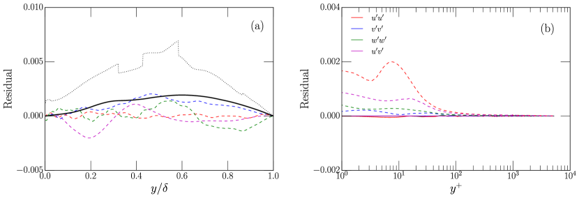
Figure 1: Statistical stationary of simulation: (a) Residual in (1), with linestyle legend given in Table 1 and the dotted line is the standard deviation of estimated total stress in LM5200; (b) Residual in (2) of LM5200 (solid), and the standard deviation of the estimated statistical error in the sum of the RHS terms in (2) (dashed).

3 Results

In the discussion to follow, when comparing results from different simulations, data from the three cases with the highest Reynolds number (LM5200, LJ4200 and BPO4100) are plotted with solid lines while the lower Reynolds number cases are with dashed lines. The experimental data are plotted with symbols. The legend of line styles, colors and symbols is given in Table 1.

3.1 Mean velocity profile

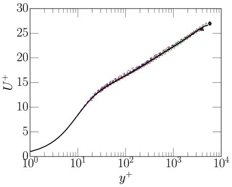
Figure 2: Mean streamwise velocity profile for all the cases listed in Table 1, where the legend of line styles and symbols is also given.

The multi-scale character of wall bounded turbulence, in which $\nu/u_{\tau}$ is the length scale relevant to the near-wall flow and $\delta$ applies to the flow away from the wall, is well known. As first noted by Millikan (1938), this scaling behavior and asymptotic matching lead to the logarithmic variation of mean streamwise velocity with the distance from the wall in an overlap region between the inner and outer flow. This “log law” is given by

$$U^{+}=\frac{1}{\kappa}\log y^{+}+B$$ (3)

where $\kappa$ is the von Kármán constant. In a log layer, the indicator function

$$\beta(y^{+})=y^{+}\frac{\partial U^{+}}{\partial y^{+}}$$

is constant and equal to $1/\kappa$. Hence, the indicator function, $\beta$, will have a plateau if there is a logarithmic layer.

The mean streamwise velocity profile is shown in figure 2 for all the data sets listed in Table 1. The profiles from all the relatively high Reynolds number cases are consistent as expected. Despite this agreement, the indicator function $\beta$ shows some disagreement between the three highest Reynolds number simulations, as shown in figure 3(a). In the LM5200 case, $\beta$ is approximately flat between $y^{+}=350$ and $y/\delta=0.16$ ($y^{+}=830$), indicating a log-layer in this region. The LJ4200 case also appears to be converging toward a plateau in this region, but there is apparent statistical noise in the profile, which is understandable given the small domain size. However, the BPO4100 simulation does not have a plateau in $\beta$. There is also a small discrepancy between BPO4100 and the other two cases from $y^{+}\approx 30$ to 100. These discrepancies are significantly larger than the statistical uncertainty in the value of $\beta$ (approximately 0.2%) in the current simulations, and presumable in the BPO4100 simulations, as the averaging time and domain sizes are comparable.

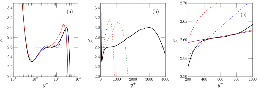
Figure 3: Log-law indicator function $\beta$ for (a) the highest Reynolds number simulations, LM5200, LJ4200 and BPO4100, (b) simulations at $Re_{\tau}=5186$, 2003 and 1000 (LM5200, HJ2000 and LM1000), and (c) simulation LM5200 along with the expressions (4, blue) and (5, red). In (a), the horizontal dashed line is at $\beta=1/\kappa=1/0.384$, and in (c) parameter values (see Table 2) fit from LM5200 are solid, and from Jiménez & Moser (2007); Mizuno & Jiménez (2011) are dashed. The linestyle legend for (a) and (b) is given in Table 1.

The values of $\kappa$ and $B$ in (3) were determined by fitting the mean velocity data from LM5200 in the region between $y^{+}=350$ and $y/\delta=0.16$ to obtain the values of $0.384\pm 0.004$ and 4.27, respectively, with $R^{2}=0.9999$ where $R^{2}$ is the coefficient of determination, which is one for a perfect fit. The value of $\kappa$ agrees with the value computed by Lozano-Durán & Jiménez (2014), but shows a slight discrepancy with the values measured by Nagib & Chauhan (2008) and Monty (2005), which are $\kappa=0.37$ and 0.39, respectively. The value of $\kappa$ obtained here is remarkably similar to that reported by Österlund et al. (2000), $\kappa=0.38$, and, Nagib & Chauhan (2008), $\kappa=0.384$, in the zero pressure gradient boundary layer. However, the value of $\kappa$ reported here is smaller than $\kappa=0.40$ measured by Bailey et al. (2014) in pipe flow. Note that choosing the range for this curve fit is somewhat arbitrary, since the indicator function is not exactly flat (figure 3c).

From an asymptotic analysis perspective, the log-law relation (3) is the lowest order truncation of a matched asymptotic expansion in $1/Re_{\tau}$ (Afzal & Yajnik, 1973; Jiménez & Moser, 2007). Several higher order representations of the mean velocity in the overlap region have been evaluated based on experimental and DNS data in boundary layers, channels and pipes (Buschmann & Gad-el-Hak, 2003; Jiménez & Moser, 2007; Mizuno & Jiménez, 2011). Here we consider two such applications to channels in the context of the LM5200 data.

Jiménez & Moser (2007) considered a higher order truncation in which $\beta$ has the form:

$$\beta=y^{+}\frac{\partial U^{+}}{\partial y^{+}}=\left(\frac{1}{\kappa_{\infty}}+\frac{\alpha_{1}}{Re_{\tau}}\right)+\alpha_{2}\frac{y^{+}}{Re_{\tau}}$$ (4)

This formulation essentially allows for an $Re_{\tau}$ dependence of $\kappa=(1/\kappa_{\infty}+\alpha_{1}/Re_{\tau})^{-1}$, and introduces a linear dependence on $y/\delta=y^{+}/Re_{\tau}$. Based on data from a simulation at $Re_{\tau}\approx 1000$ by Del Álamo et al. (2004) (similar to LM1000) and from HJ2000, (see figure 3b), they determined the parameter values shown in table 2. Further, this form and these values were found to be consistent with experimental measurements by Christensen & Adrian (2001) at Reynolds numbers up to $Re_{\tau}=2433$.

Mizuno & Jiménez (2011) considered a different higher-order asymptotic truncation, for which $\beta$ is given by:

$$\beta=y^{+}\frac{\partial U^{+}}{\partial y^{+}}=\frac{y^{+}}{\kappa(y^{+}-a_{1})}+a_{2}\frac{y^{+2}}{Re_{\tau}^{2}}.$$ (5)

The second term was motivated by the form of a wake model that is quadratic for small $y/\delta$, where the coefficient is related to the wake parameter $\Pi$ by $a_{2}=(12\Pi-2)/\kappa$. The term $a_{1}$ is an offset (virtual origin) which accounts for the presence of the viscous layer (Wosnik et al., 2000). To first order in $a_{1}/y^{+}$, the offset is equivalent to including an additive $a_{1}/\kappa y^{+}$ term, which is expected from the matched asymptotics. They fit the inverse of the mean velocity derivative to $y^{+}/\beta$ from (5) using the experimental and DNS data mentioned above and the experiments of Monty (2005), with up to $Re_{\tau}=3945$, to determine a Reynolds number dependent value of the parameters. When evaluated for $Re_{\tau}=5186$, these yield the parameter values shown in table 2.

Equation (4)				Equation (5)
	Jiménez & Moser (2007)	LM5200			Mizuno & Jiménez (2011)	LM5200
$\kappa_{\infty}$	000.4020			$\Pi$	000.179	00.189
$\alpha_{1}$	150.0000			$a_{1}$	-12.400	-1.000
$\alpha_{2}$	001.0000	0.2000		$a_{2}$	000.394	00.700
$\kappa$	000.3970	0.3867		$\kappa$	000.363	00.384

Table 2: Values of parameters in (4) and (5) appropriate for $Re_{\tau}=5186$ as determined by Jiménez & Moser (2007); Mizuno & Jiménez (2011) and from the LM5200 data.

These two higher-order truncations have also been fit to the LM5200 data to obtain values shown in table 2, which are significantly different from the previously determined values. The expressions for $\beta$ from (4) and (5) are plotted in figure 3(c) with both sets of parameters. It is clear from this figure that the parameter values obtained by Jiménez & Moser (2007) and Mizuno & Jiménez (2011) do not fit the LM5200 data, but the parameters fit to the LM5200 data in the log region match the data equally well for both truncation forms. The reason for this disagreement with the parameters from Jiménez & Moser (2007) is clear, since the Reynolds numbers used in that study were not high enough to exhibit the logarithmic region observed in LM5200, since $y/\delta=0.16$ is at $y^{+}=320$ when $Re_{\tau}=2000$. They appear to have been fitting (4) to the outer-layer profile, and indeed in LM5200 there is a region $0.16<y/\delta<0.45$ in which $\beta$ is approximately linear in $y^{+}/Re_{\tau}$, with slope of one (figure 3b), in agreement with $\alpha_{2}=1.0$.

In contrast, the data used by Mizuno & Jiménez (2011) included a channel Reynolds number as high as $Re_{\tau}=3945$, which should have exhibited a short nearly constant $\beta$ plateau as observed in LM5200. This would have been qualitatively different from the lower Reynolds number cases. This was not reported in in that paper. But, at this Reynolds number, the plotted values of $\kappa$ and $a_{1}$ (figure 5 in Mizuno & Jiménez (2011)) are significantly larger than the parameters for lower Reynolds number. Further, the values for all three parameters obtained from the LM5200 data are within the indicated uncertainties of the parameters from the $Re_{\tau}=3945$ experimental data. Perhaps the reported Reynolds number dependence of the parameters did not reflect a qualitative change at the highest Reynolds number, because the fit was dominated by the more numerous lower Reynolds number cases.

The apparent extent of the overlap region in the LM5200 case is not sufficient to distinguish between the two asymptotic truncations, (4) and (5). Because $a_{1}$ is so small, the primary distinction is in the lowest non-zero exponent on $y^{+}/Re_{\tau}$. This may be of some importance because it determines the way the high Reynolds number asymptote of constant $\beta$ is approached. Unfortunately, this cannot be determined using the available data.

3.2 Reynolds Stress Tensor

The non-zero components of the Reynolds stress tensor (the velocity component variances and co-variance) from the simulations and experiments are shown in Figs. 4–6. These figures show that there are some subtle inconsistencies among the three highest Reynolds number simulations (solid lines in the figures) and the experimental data.

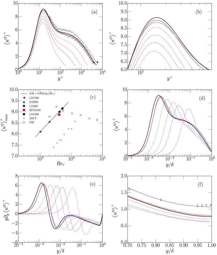
Figure 4: Variance of $u$: (a) as a function of $y^{+}$; (b) zoom of (a) near the peak; (c) dependence of maximum on $Re_{\tau}$; Solid line, relation; (6); MWT, boundary layer in the Melbourne Wind Tunnel (Hutchins et al., 2009; Kulandaivelu, 2011); PSP, Princeton Superpipe Hultmark et al. (2010, 2012); (d) as a function of $y/\delta$; (e) test function for Townsend’s prediction; and, (f) zoom of (d) near the center of channel. The linestyle and symbol legend is given in Table 1.

First, the two cases LJ4200 and BPO4100 are nearly identical in Reynolds number, but all three velocity variances are different between the two cases. The peak of the streamwise variance (Fig. 4b) is about 1.4% larger in LJ4200 than in BPO4100. The peak varies with Reynolds number, as can be seen in the figure, but this variation is logarithmic, and is too weak to explain the difference. Using the simulations LM1000, HJ2000 and LM5200, the dependence of the peak in $\langle u^{\prime 2}\rangle^{+}$ on $Re_{\tau}$ was fit to get

$$\langle u^{\prime 2}\rangle^{+}_{max}=3.66+0.642\log\left(Re_{\tau}\right)$$ (6)

with $R^{2}=0.9995$. This agrees well with the relationship, $\langle u^{\prime 2}\rangle^{+}_{max}=3.63+0.65\log\left(Re_{\tau}\right)$, suggested by Lozano-Durán & Jiménez (2014). The relationship (6) is plotted in Fig 4c along with the values of the actual peaks, including those for LJ4200 and BPO4100. It is clear from this plot that the peak in BPO4100 is smaller than this relationship implies for $Re_{\tau}=4100$, while the peak from LJ4200 is consistent.

Also shown in Fig 4(c) are experimental data for pipe flow by Hultmark et al. (2010, 2012), which indicate that the inner-peak value of $\left<u^{\prime 2}\right>^{+}$ does not continue to increase with $Re$ for $Re_{\tau}>5000$. However, experimental data from boundary layers by (Hutchins et al., 2009; Kulandaivelu, 2011) do not show such a growth saturation. The Reynolds numbers of the current simulations are unfortunately not high enough to determine whether the growth of $\left<u^{\prime 2}\right>^{+}$ will saturate in channel flows. Also remarkable in Fig 4(c) is how much lower the peak values are in the boundary layer data. This is likely due to the resolution of the measurements (Hutchins et al., 2009).

In other $y^{+}$ intervals ($y^{+}<8$ and $25<y^{+}<200$), the variance in the lower Reynolds number case (BPO4100) is actually greater than the variance in the higher Reynolds number flow (LJ4200). This appears to be inconsistent with the Reynolds number trends among the other cases, for which $\langle u^{\prime 2}\rangle^{+}$ is monotonically increasing with Reynolds number at constant $y^{+}$. Another inconsistency is apparent when the streamwise velocity variance is examined as a function of $y/\delta$ (Fig. 4d,f). Near the centerline ($y/\delta=1$), the variance from LJ4200 is significantly larger than for both BPO4100 and LM5200, while the other simulations indicate that variance should be increasing slowly with Reynolds number. It appears that far from the wall, LJ4200 is affected by its relatively small domain size, as might be expected. Finally, the experimental data with reported uncertainty, $\pm$ 2%, from SF4000 in Fig 4a is inconsistent with LJ4200 and BPO4100 in the region near the wall ($y^{+}<300$ say). The reason for this discrepancy is not clear, but it may be due to the difficulty of measuring velocity fluctuations near the wall. Far from the wall, the experimental data for these quantities is consistent with the simulations. Measurements are not available at small enough $y^{+}$ to compare peak values of $\langle u^{\prime 2}\rangle^{+}$.

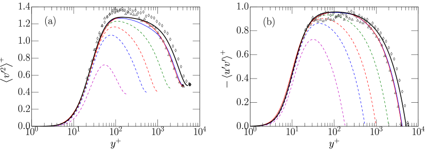
Figure 5: Variance of $v$ (a) and covariance of $u$ and $v$ (b). The linestyle and symbol legend is given in Table 1

.

Similar inconsistencies are present among the high Reynolds number simulation cases in the wall-normal and spanwise velocity variances. Around the peaks of both $\langle v^{\prime 2}\rangle^{+}$ and $\langle w^{\prime 2}\rangle^{+}$, BPO4100 exceeds values from LJ4200, despite its somewhat lower Reynolds number (Fig. 5a and Fig. 6a), while near the center, these two cases are in agreement. Only the Reynolds shear stress $\langle u^{\prime}v^{\prime}\rangle^{+}$ is in agreement in these cases across all $y$ (Fig 5b). Similar to $\langle u^{\prime 2}\rangle^{+}$, the experimental data from SF4000 for $\langle v^{\prime 2}\rangle^{+}$ and $\langle u^{\prime}v^{\prime}\rangle^{+}$ with uncertainties, $\pm$ 3% and $\pm$ 5%, respectively, are inconsistent with both simulations in the region near the wall, where the experimental data appears to be quite noisy. Possible reasons for the minor inconsistencies noted among the DNS are discussed in §3.3.

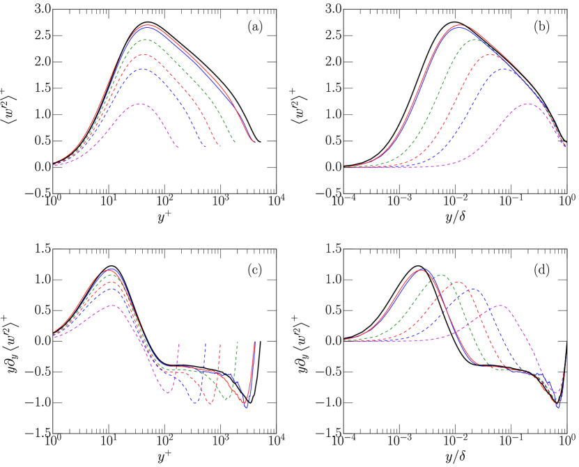
Figure 6: Variance of $w$ (a) as a function of $y^{+}$ (b) as a function of $y/\delta$, and test function for Townsend’s prediction (c) as a function of $y^{+}$ (d) as a function of $y/\delta$. The linestyle and symbol legend is given in Table 1.

There are several anticipated high-Reynolds-number features to be examined in this data. In particular, similar to the log law, Townsend’s attached eddy hypothesis (Townsend, 1976) implies that in the high Reynolds number limit, there is an interval in $y$ in which the Reynolds stress components satisfy ⟨u^′2⟩^+ & = A_1 - B_1 log(y/δ)
⟨v^′2⟩^+ = A_2
⟨w^′2⟩^+ = A_3 - B_3 log(y/δ)
⟨u’v’ ⟩^+ = -1 Consistent with these relations, both $\langle v^{\prime 2}\rangle^{+}$ and $-\langle u^{\prime}v^{\prime}\rangle^{+}$ are developing a flat region as Reynolds number increases (Fig 5), though the maximum Reynolds shear stress is well bellow one (0.96). Because the total stress

$$\tau_{\rm tot}=\nu\frac{\partial U}{\partial y}-\langle u^{\prime}v^{\prime}\rangle$$ (7)

is known analytically ($\tau^{+}_{\rm tot}=1-y/\delta$) from the mean momentum equation, and because $\beta$ varies little over a broad range of $y$ ($\beta=2.6\pm 0.4\approx 1/\kappa$ for $30<y^{+}<0.75Re_{\tau}$ (see Fig. 3), the variation with Reynolds number of the Reynolds shear stress near its maximum can be deduced easily:

$$\tau_{RS}^{+}=-\langle u^{\prime}v^{\prime}\rangle^{+}\approx 1-\frac{y^{+}}{Re_{\tau}}-\frac{1}{\kappa y^{+}}\quad\mbox{for}\quad 30<y^{+}<0.75Re_{\tau}$$ (8)

From this it is clear that the maximum Reynolds shear stress is given by $\tau_{RS{\rm max}}\approx 1-2/\sqrt{\kappa Re_{\tau}}$, and that this maximum occurs at $y^{+}\approx\sqrt{Re_{\tau}/\kappa}$ as noted by Afzal (1982), Morrison et al. (2004), Panton (2007) and Sillero et al. (2013). For the conditions of LM5200 ($Re_{\tau}=5186$, $\kappa=0.384$), these estimates yield $\tau_{RS{\rm max}}\approx 0.955$ occurring at $y^{+}\approx 116$, in good agreement with the simulations. Further, the error in satisfying $\tau_{RS}=1$ is less than $\epsilon$ for a range of $y^{+}$ that increases in size like $\epsilon Re_{\tau}$ for large $Re_{\tau}$. Precisely:

$$1-\tau_{RS}<\epsilon\quad\mbox{provided}\quad\left|y^{+}-\frac{\epsilon Re_{\tau}}{2}\right|<\frac{\epsilon Re_{\tau}}{2}\sqrt{1-\frac{4}{\epsilon^{2}Re_{\tau}\kappa}}.$$ (9)

Thus, for $\tau_{RS}$ to be within 5% of one over a decade of variation of $y^{+}$ would require more than twice the Reynolds number of LM5200, and for it to be within 1% at its peak requires 20 times greater Reynolds number.

According to (6), both the variance of $u$ and the variance of $w$ would have a logarithmic variation over some region of $y$. In Fig. 6, it appears that there is such a logarithmic variation, even at Reynolds numbers as low as $Re_{\tau}=1000$. The indicator function $y\partial_{y}\langle w^{\prime 2}\rangle$ is approximately flat from $y^{+}\approx 100$ to $y^{+}\approx 200$ (Fig. 6c). The corresponding curve fit is $\langle w^{\prime 2}\rangle^{+}=1.08-0.387\log(y/\delta)$, which is somewhat different from the fit $\langle w^{\prime 2}\rangle^{+}=0.8-0.45\log(y/\delta)$ obtained by Sillero et al. (2013) in a boundary layer DNS. On the other hand, there is no apparent logarithmic region in the $\langle u^{\prime 2}\rangle^{+}$ profiles. The indicator function $y\partial_{y}\langle u^{\prime 2}\rangle^{+}$ (Fig. 4e) is not flat anywhere in the domain. There is however a region ($200<y^{+}<0.6Re_{\tau}$), where the dependence of the indicator function on $y$ is linear with relatively small slope, and the slope may be decreasing with Reynolds number, though extremely slowly. In contrast, Hultmark et al. (2012, 2013) observed a logarithmic region in $\langle u^{\prime 2}\rangle^{+}$ over the range $800<y^{+}<0.15Re_{\tau}$ in pipe flow with $Re_{\tau}>2\times 10^{4}$. The LM5200 simulation is not at high enough Reynolds number to exhibit such a region if it occurs over the same range in $y$, since $0.15Re_{\tau}<800$ at $Re_{\tau}=5186$.

As mentioned in §2, the terms in the Reynolds stress transport equations are not reported here, though the data are available at http://turbulence.ices.utexas.edu. Of interest here, however, is the transport equation for the turbulent kinetic energy $K=\frac{1}{2}\langle u^{\prime}_{i}u^{\prime}_{i}\rangle$. Hinze (1975) argues that at sufficiently high Reynolds number, there is an intermediate region between inner and outer layers where the transport terms in the kinetic energy equation are small compared to production so that in this region

$$P_{K}\approx{\epsilon},$$ (10)

where $P_{K}$ is the production of kinetic energy and $\epsilon$ is the dissipation. In the formulation and analysis of turbulence models, (10) is often assumed to hold in an overlap region between inner and out layers (Durbin & Pettersson Reif, 2010). The relative error in the balance of production and dissipation ($P_{K}/\epsilon-1$) for LM1000, HJ2000 and LM5200, is shown in figure 7. In all three cases, there is a region $y^{+}>30$ and $y/\delta<0.6$ in which the mismatch between production and dissipation is of order 10% or less, but there is no indication that the magnitude of this mismatch is decreasing with Reynolds number. Indeed, there appears to be a stable structure with a local minimum in $P_{K}/\epsilon$ around $y^{+}=60$ and a local maximum around $y^{+}=300$ followed by a gradual decline toward $P_{K}/\epsilon=1$ with increasing $y$. Presumably this decline will become more gradual with increasing Reynolds number as $y/\delta=0.6$ increases in $y^{+}$.

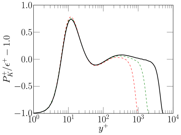
Figure 7: Balance of production and dissipation of turbulent kinetic energy

3.3 Discrepancies Between Simulations

In §3.1 and §3.2, it was shown that the LM5200 simulation has differences from the two somewhat lower Reynolds number DNS LJ4200 and BPO4100, with discrepancies among all three simulations larger than expected given the Reynolds number differences and likely statistical errors. In the case of LJ4200, the reason for the differences with LM5200 is most likely the small domain size of LJ4200 (four and three times smaller in the streamwise and spanwise directions respectively). Indeed Lozano-Durán & Jiménez (2014) investigated the effects of the small domain size at $Re_{\tau}\approx 950$ by comparing to DNS in a domain consistent with the simulations reported here. Consistent with observations in §3.2, they observed discrepancies in the velocity variances for $y/\delta<0.25$.

The differences between BPO4100 and both LJ4200 and LM5200 occur primarily in the near-wall region, as shown in §3.2. It seems likely that these differences are due to numerical resolution limitations of BPO4100. As indicated in Table 1, the grid spacing in BPO4100 is about the same as LM5200 in the spanwise direction and about 25% finer in the streamwise direction. However, in BPO4100 a second order finite difference approximation is used rather than the spectral method used in the simulations reported here. The effective resolution of such low-order schemes is significantly less at the same grid spacing. One way to see this is to consider the error incurred when differentiating a sine function of different wavenumbers, which is given by $\epsilon(k)=1-\sin(k\Delta)/k\Delta$. If one insists on limiting error to no more than 10% (for example), then the wavenumber needs to be limited to one fourth of the highest wavenumber that can be represented on the grid. Thus, at this level of error, the finite difference approximation of the derivative has four times coarser effective resolution than a spectral method on the same grid.

Of course, there is much more to solving the Navier-Stokes equations than representing the derivative and an appropriate error limit for the derivative is not clear. None-the-less, in DNS, a common rule of thumb is that second order finite difference has between two to four times coarser effective resolution than a Fourier spectral method on the same grid. In a study of the effects of resolution in DNS of low Reynolds number ($Re_{\tau}=180$) channel flow, Oliver et al. (2014) found that with the Fourier/B-spline numerical representation used here, coarsening the resolution by a factor of two relative to the nominal resolution (nominal is comparable in wall units to that used for LM5200) results in changes of several percent in the velocity variances near the wall. Further, Vreman & Kuerten (2014) investigated differences between DNS using a Fourier-Chebyshev spectral method and DNS using a fourth order staggered finite difference method, which is higher order and higher resolution than the method used for BPO4100. They reported a 1% lower peak rms $u^{\prime}$ for the fourth-order method. These results indicate that the lower effective resolution in BPO4100 relative to LM5200 is a plausible cause for the minor inconsistencies between these two simulations. To determine this definitively would require redoing the BPO4100 simulation with twice the resolution in each direction, or more, which is out of scope for the current study.

3.4 Energy spectral density

One of the properties of high-Reynolds-number wall-bounded turbulence is the separation of scales between the near-wall and outer-layer turbulence. For the LM5200 case, this separation of scales can be seen in the one-dimensional velocity spectra. For example, the premultiplied spectral energy density of the streamwise velocity fluctuations is shown as a function of $y$ in figure 8. The pre-multiplied spectrum $kE(k,y^{+})$ is the energy density per $\log k$ and so, in the logarithmic wavenumber scale used in figure 8, it indicates the scales at which the energy resides. The energy spectral density of $u$ in the streamwise direction has two distinct peaks, one at $k_{x}\delta=40$, $y^{+}=13$ and one at $k_{x}\delta=1$, $y^{+}=400$. To our knowledge, such distinct peaks have only previously been observed in high Reynolds number experimental data (Hutchins & Marusic, 2007; Monty et al., 2009; Marusic et al., 2010a, b). An even more vivid double peak is visible in the spanwise spectrum of $u$ (figure 8b), with peaks at $k_{z}\delta=250$, $y^{+}=13$ and at $k_{z}\delta=6$, $y^{+}=1000$.

Similarly there are weak double peaks in the cospectrum of $uv$ as shown in figure 8c,d. In the LM5200 case, distinct inner and outer peaks were not observed in the spectral density of $v^{2}$ and $w^{2}$ (not shown). It thus appears that it is primarily the streamwise velocity fluctuations that are exhibiting inner/outer scale separation at this Reynolds number.

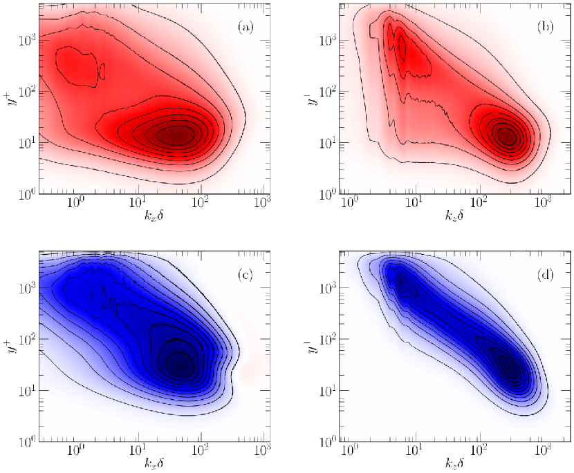
Figure 8: Wavenumber-premultiplied energy spectral density, LM5200 (a) $k_{x}E_{uu}/u_{\tau}^{2}$ (b) $k_{z}E_{uu}/u_{\tau}^{2}$ (c) -$k_{x}E_{uv}/u_{\tau}^{2}$ (d) -$k_{z}E_{uv}/u_{\tau}^{2}$

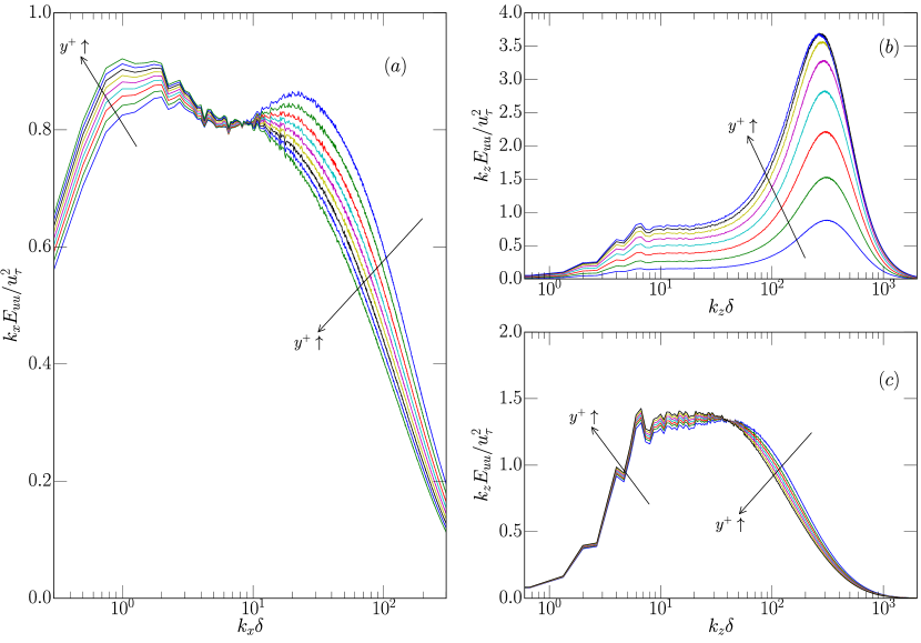
Figure 9: $k^{-1}$ region (a) $k_{x}E_{uu}/u_{\tau}^{2}$ at $y^{+}=90\sim 170$ (b) $k_{z}E_{uu}/u_{\tau}^{2}$ at $y^{+}=3\sim 14$ (c) $k_{z}E_{uu}/u_{\tau}^{2}$ at $y^{+}=111\sim 141$

As mentioned earlier, the scaling analysis of Perry et al. (1986) suggests that at high Reynolds number the energy spectral density of the streamwise velocity fluctuations varies as $k_{x}^{-1}$ in the overlap region where both inner and out scaling is valid. However, until now, the $k_{x}^{-1}$ region has been elusive in simulations, presumably because the Reynolds numbers have not been high enough. It is only in high Reynolds number experiments (Nickels et al., 2005, 2007; Rosenberg et al., 2013) that a $k_{x}^{-1}$ regions has previously been observed in the streamwise velocity spectrum. In the LM5200 simulation, the premultiplied energy spectral density does indeed exhibit a plateau in the region $90\leq y^{+}\leq 170$ and $6\leq k_{x}\delta\leq 10$ (figure 9 (a)). Further, the magnitude of the premultiplied spectrum at the plateau agrees with the value observed experimentally, about 0.8 in wall units, in boundary layers (Nickels et al., 2005) and in pipe flow (Rosenberg et al., 2013). However, the plateau in the experimental premultiplied spectrum in the pipe flow of Rosenberg et al. (2013) is only observed for $Re_{\tau}\leq 3300$. From the current results, we cannot determine whether the occurrence or extent of the plateau region might change at higher Reynolds number in channels.

A similar scaling analysis also suggests that there should be a plateau in the premultiplied spanwise spectrum, and indeed an even broader plateau appears for $5\leq k_{z}\delta\leq 30$, as observed previously by Hoyas & Jiménez (2008) and Sillero et al. (2013). Interestingly, the plateau also occurs in the viscous sub-layer region (figure 9 (b)). In the viscous sub-layer the streamwise velocity fluctuations are dominated by the well-known streaky structures, with a characteristic spacing of $\Delta z^{+}\approx 100$. This is evidenced by the large high-wavenumber peaks in the spanwise spectra around $k_{z}/\delta\approx 300$ ($k_{z}^{+}\approx 2\pi/\Delta z^{+}$). At much larger scales (much lower wavenumbers), the viscous layer is driven by the larger-scale turbulence further from the wall. The plateau in the spanwise premultiplied spectrum in the viscous layer is thus a reflection of the spectral plateau further from the wall (figure 9 (c)).

Another experimentally observed feature of the streamwise premultiplied spectrum is the presence of two local maxima, with one peak occurring on either side of the plateau (Guala et al., 2006; Kunkel & Marusic, 2006). However, this bi-modal feature was called into question when it was noted that the low-wavenumber peak, which occurs at $k_{x}\delta$ of order one, is at low enough wavenumber to be affected by the use of Taylor’s hypothesis to infer the spatial spectrum from the measured temporal spectrum (Del Álamo & Jiménez, 2009; Moin, 2009). Indeed, in the HJ2000 simulation, it was found that the streamwise spatial spectrum did not display a low-wavenumber peak, while a spectrum determined from a time series did (Del Álamo & Jiménez, 2009). In the LM5200 case, this bi-modal feature does occur, as can be seen in figure 9 (a). However, it is not clear whether this is a general high Reynolds number feature, or whether it is characteristic of intermediate Reynolds numbers. From figure 8, it is clear that the high and low wavenumber peaks in $k_{x}E_{uu}(k_{x},y^{+})$ at around $y^{+}=100$ are simply the upper and lower edges of the near-wall and outer peaks in $k_{x}E_{uu}(k_{x},y^{+})$, respectively. As the Reynolds number increases, the inner peak will move to larger $k_{x}$ and the outer peak to larger $y^{+}$. As the outer peak moves to larger $y^{+}$, it seems likely that the inner and outer peaks will not overlap at all in $y$, resulting in no bi-modal pre-multiplied spectrum at any $y$. For example, the peaks are better separated in the premultiplied spanwise spectrum, and there are no bi-modal $k_{z}$ pre-multiplied spectra (figure 9 (b)).

4 Discussion and Conclusion

The direct numerical simulation of turbulent channel flow at $Re_{\tau}=5186$ that is reported here has been shown to be a reliable source of data on high Reynolds number wall-bounded turbulence, and a wealth of statistical data from this flow is available on line at http://turbulence.ices.utexas.edu. In particular: resolution is consistent with or better than accepted standards for wall-bounded turbulence DNS; statistical uncertainties are generally small (of order 1% or less), statistical data is consistent with Reynolds number trends in DNS at $Re_{\tau}\leq 2000$, and with experimental data, within reasonable tolerance; and, finally, the flow is statistically stationary to high accuracy. Further, as recapped below, the simulation exhibits many characteristics of high Reynolds number wall-bounded turbulence, making this simulation a good resource for the study of such high Reynolds number flows. Several conclusions can thus be drawn about high Reynolds number turbulent channel flow as discussed below.

At high Reynolds number, it is expected that a region of logarithmic variation will exist in the mean velocity. The current simulation exhibits an unambiguous logarithmic region with von Kármán constant $\kappa=0.384\pm 0.004$. This is the first such unambiguous simulated logarithmic profile that the authors are aware of. At high Reynolds number, it is also expected (Townsend, 1976) that the variance of the velocity fluctuations will have a region of logarithmic variation. This was found to be true for the spanwise fluctuations, but not the streamwise fluctuations. Indeed, the streamwise variance shows no sign of converging towards a logarithmic variation with increasing Reynolds number. Finally, it is often assumed that at high Reynolds number the production of turbulent kinetic energy will locally balance its dissipation over some overlap region between inner and outer layers. However, this was observed only approximately in the current simulation, with 10% accuracy and with no sign that that this miss-match is declining with Reynolds number. This balance of production and dissipation thus appears to be just an imperfect approximation.

One of the most important characteristics of high Reynolds number wall-bounded turbulence is a distinct separation in scale between turbulence near the wall and far from the wall. This was observed in the streamwise and spanwise premultiplied spectral density of the streamwise velocity fluctuations and in the co-spectrum of streamwise and wall-normal fluctuations. Also, a short $k^{-1}$ region is observed in the streamwise spectra and there is a wider region in the spanwise spectra, as predicted from scaling analysis (Perry et al., 1986), and as observed experimentally. Finally, the bi-modal structure in the premultiplied spectrum that has been observed experimentally (Guala et al., 2006; Kunkel & Marusic, 2006) has also been observed here, despite suggestions that the experimental observations were an artifact of the use of Taylor’s hypothesis, which is not used here. However, it seems likely that this two-peak structure will not continue as the Reynolds number increases and the inner and outer peaks in the premultiplied spectra become further separated in $k$ and in $y$.

5 Acknowledgment

The work presented here was supported by the National Science Foundation under Award Number [OCI-0749223] and the Argonne Leadership Computing Facility at Argonne National Laboratory under Early Science Program(ESP) and Innovative and Novel Computational Impact on Theory and Experiment Program(INCITE) 2013. We wish to thank N. Malaya and R. Ulerich for software engineering assistance. We are also thankful to M. P. Schultz and K. A. Flack for providing their experimental data.

References

- Afzal (1976) Afzal, Noor 1976 Millikan’s argument at moderately large Reynolds number. Physics of Fluids 19 (4), 600–602.
- Afzal (1982) Afzal, Noor 1982 Fully developed turbulent flow in a pipe: an intermediate layer. Ingenieur-Archiv 52, 355–377.
- Afzal & Yajnik (1973) Afzal, N. & Yajnik, K. 1973 Analysis of turbulent pipe and channel flows at moderately large reynolds number. J. Fluid Mech. 61, 23–31.
- Bailey et al. (2014) Bailey, S. C. C., Vallikivi, M., Hultmark, M. & Smits, A. J. 2014 Estimating the value of von Kármán’s constant in turbulent pipe flow. Journal of Fluid Mechanics 749, 79–98.
- Bernardini et al. (2014) Bernardini, Matteo, Pirozzoli, Sergio & Orlandi, Paolo 2014 Velocity statistics in turbulent channel flow up to = 4000. Journal of Fluid Mechanics 742, 171–191.
- Borrell et al. (2013) Borrell, Guillem, Sillero, Juan a. & Jiménez, Javier 2013 A code for direct numerical simulation of turbulent boundary layers at high Reynolds numbers in BG/P supercomputers. Computers & Fluids 80, 37–43.
- Botella & Shariff (2003) Botella, Olivier & Shariff, Karim 2003 B-spline Methods in Fluid Dynamics. International Journal of Computational Fluid Dynamics 17 (2), 133–149.
- Buschmann & Gad-el-Hak (2003) Buschmann, Matthias H. & Gad-el-Hak, Mohamed 2003 Generalized Logarithmic Law and Its Consequences. AIAA Journal 41 (1), 40–48.
- Christensen & Adrian (2001) Christensen, K. T. & Adrian, R. J. 2001 Statistical evidence of hairpin vortex packets in wall turbulence. Journal of Fluid Mechanics 431, 433–443.
- Comte-Bellot (1963) Comte-Bellot, Geneviève 1963 Contribution à l’étude de la turbulence de conduite. PhD thesis, University of Grenoble, France.
- Dean & Bradshaw (1976) Dean, R. B. & Bradshaw, P. 1976 Measurements of interacting turbulent shear layers in a duct. Journal of Fluid Mechanics 78, 641–676.
- DeGraaff & Eaton (2000) DeGraaff, D. B. & Eaton, J. K. 2000 Reynolds-number scaling of the flat-plate turbulent boundary layer. Journal of Fluid Mechanics 422, 319–346.
- Del Álamo & Jiménez (2009) Del Álamo, Juan C. & Jiménez, Javier 2009 Estimation of turbulent convection velocities and corrections to Taylor’s approximation. Journal of Fluid Mechanics 640, 5–26.
- Del Álamo et al. (2004) Del Álamo, Juan C., Jiménez, Javier, Zandonade, Paulo & Moser, Robert D. 2004 Scaling of the energy spectra of turbulent channels. Journal of Fluid Mechanics 500, 135–144.
- Durbin & Pettersson Reif (2010) Durbin, P. A. & Pettersson Reif, B. A. 2010 Statistical Theory and Modeling for Turbulent Flows. John Wiley & Sons, Ltd.
- El Khoury et al. (2013) El Khoury, George K., Schlatter, Philipp, Noorani, Azad, Fischer, Paul F., Brethouwer, Geert & Johansson, Arne V. 2013 Direct Numerical Simulation of Turbulent Pipe Flow at Moderately High Reynolds Numbers. Flow, Turbulence and Combustion 91 (3), 475–495.
- Fernholz & Finley (1996) Fernholz, H. H. & Finley, P. J. 1996 The incompressible zero-pressure-gradient turbulent boundary layer: an assessment of the data. Progress in Aerospace Sciences 32 (8), 245–311.
- Guala et al. (2006) Guala, M., Hommema, S. E. & Adrian, R. J. 2006 Large-scale and very-large-scale motions in turbulent pipe flow. Journal of Fluid Mechanics 554, 521–542.
- Hinze (1975) Hinze, J. O. 1975 Turbulence. McGraw-Hill Book Company, Inc.
- Hoyas & Jiménez (2006) Hoyas, Sergio & Jiménez, Javier 2006 Scaling of the velocity fluctuations in turbulent channels up to =2003. Physics of Fluids 18 (1), 011702.
- Hoyas & Jiménez (2008) Hoyas, Sergio & Jiménez, Javier 2008 Reynolds number effects on the Reynolds-stress budgets in turbulent channels. Physics of Fluids 20 (10), 101511.
- Hultmark et al. (2010) Hultmark, Marcus, Bailey, Sean C. C. & Smits, Alexander J. 2010 Scaling of near-wall turbulence in pipe flow. Journal of Fluid Mechanics 649, 103–113.
- Hultmark et al. (2012) Hultmark, M., Vallikivi, M., Bailey, S. C. C. & Smits, A. J. 2012 Turbulent Pipe Flow at Extreme Reynolds Numbers. Physical Review Letters 108, 094501.
- Hultmark et al. (2013) Hultmark, M., Vallikivi, M., Bailey, S. C. C. & Smits, A. J. 2013 Logarithmic scaling of turbulence in smooth- and rough-wall pipe flow. Journal of Fluid Mechanics 728, 376–395.
- Hutchins et al. (2012) Hutchins, Nicholas, Chauhan, Kapil, Marusic, Ivan, Monty, Jason & Klewicki, Joseph 2012 Towards Reconciling the Large-Scale Structure of Turbulent Boundary Layers in the Atmosphere and Laboratory. Boundary-Layer Meteorology 145 (2), 273–306.
- Hutchins & Marusic (2007) Hutchins, Nicholas & Marusic, Ivan 2007 Large-scale influences in near-wall turbulence. Philosophical transactions. Series A, Mathematical, physical, and engineering sciences 365 (1852), 647–664.
- Hutchins et al. (2009) Hutchins, N., Nickels, T. B., Marusic, I. & Chong, M. S. 2009 Hot-wire spatial resolution issues in wall-bounded turbulence. Journal of Fluid Mechanics 635 (2009), 103–136.
- Jiménez & Moser (2007) Jiménez, Javier & Moser, Robert D 2007 What are we learning from simulating wall turbulence? Philosophical transactions. Series A, Mathematical, physical, and engineering sciences 365 (1852), 715–732.
- Johansson & Alfredsson (1982) Johansson, Arne V. & Alfredsson, P. Henrik 1982 On the structure of turbulent channel flow. Journal of Fluid Mechanics 122, 295–314.
- Johnson (2005) Johnson, Richard W. 2005 Higher order B-spline collocation at the Greville abscissae. Applied Numerical Mathematics 52 (1), 63–75.
- Kim et al. (1987) Kim, John, Moin, Parviz & Moser, Robert 1987 Turbulence statistics in fully developed channel flow at low Reynolds number. Journal of Fluid Mechanics 177, 133–166.
- Kim & Adrian (1999) Kim, K. C. & Adrian, R. J. 1999 Very large-scale motion in the outer layer. Physics of Fluids 11 (2), 417.
- Kulandaivelu (2011) Kulandaivelu, Vigneshwaran 2011 Evolution and structure of zero pressure gradient turbulent boundary layer. PhD thesis, University of Melbourne.
- Kunkel & Marusic (2006) Kunkel, Gary J. & Marusic, Ivan 2006 Study of the near-wall-turbulent region of the high-Reynolds-number boundary layer using an atmospheric flow. Journal of Fluid Mechanics 548, 375–402.
- Kwok et al. (2001) Kwok, Wai Yip, Moser, Robert D. & Jiménez, Javier 2001 A Critical Evaluation of the Resolution Properties of B-Spline and Compact Finite Difference Methods. Journal of Computational Physics 174 (2), 510–551.
- Lee et al. (2013) Lee, Myoungkyu, Malaya, Nicholas & Moser, Robert D. 2013 Petascale direct numerical simulation of turbulent channel flow on up to 786K cores. In Proceedings of SC13: International Conference for High Performance Computing, Networking, Storage and Analysis. New York, New York, USA: ACM Press.
- Lee et al. (2014) Lee, Myoungkyu, Ulerich, Rhys, Malaya, Nicholas & Moser, Robert D. 2014 Experiences from Leadership Computing in Simulations of Turbulent Fluid Flows. Computing in Science and Engineering 16 (5), 24–31.
- Lozano-Durán & Jiménez (2014) Lozano-Durán, Adrián & Jiménez, Javier 2014 Effect of the computational domain on direct simulations of turbulent channels up to = 4200. Physics of Fluids 26 (1), 011702.
- Marusic et al. (2010a) Marusic, Ivan, Mathis, Romain & Hutchins, Nicholas 2010a High Reynolds number effects in wall turbulence. International Journal of Heat and Fluid Flow 31 (3), 418–428.
- Marusic et al. (2010b) Marusic, I., McKeon, B. J., Monkewitz, P. A., Nagib, H. M., Smits, A. J. & Sreenivasan, K. R. 2010b Wall-bounded turbulent flows at high Reynolds numbers: Recent advances and key issues. Physics of Fluids 22 (6), 065103.
- Marusic et al. (2013) Marusic, Ivan, Monty, Jason P., Hultmark, Marcus & Smits, Alexander J. 2013 On the logarithmic region in wall turbulence. Journal of Fluid Mechanics 716, R3.
- Millikan (1938) Millikan, Clark B. 1938 A critical discussion of turbulent flows in channels and circular tubes. In Proceedings of the fifth International Congress for Applied Mechanics, pp. 386–392. J. Wiley & Sons, inc.
- Mizuno & Jiménez (2011) Mizuno, Yoshinori & Jiménez, Javier 2011 Mean velocity and length-scales in the overlap region of wall-bounded turbulent flows. Physics of Fluids 23 (8), 085112.
- Moin (2009) Moin, P. 2009 Revisiting Taylor’s hypothesis. Journal of Fluid Mechanics 640, 1–4.
- Monty (2005) Monty, J. P. 2005 Developments in smooth wall turbulent duct flows. PhD thesis, University of Melbourne.
- Monty & Chong (2009) Monty, J. P. & Chong, M. S. 2009 Turbulent channel flow: comparison of streamwise velocity data from experiments and direct numerical simulation. Journal of Fluid Mechanics 633, 461–474.
- Monty et al. (2009) Monty, J. P., Hutchins, N., Ng, H. C. H., Marusic, I. & Chong, M. S. 2009 A comparison of turbulent pipe, channel and boundary layer flows. Journal of Fluid Mechanics 632, 431–442.
- Morrison et al. (2004) Morrison, J. F., McKeon, B. J., Jiang, W. & Smits, A. J. 2004 Scaling of the streamwise velocity component in turbulent pipe flow. Journal of Fluid Mechanics 508, 99–131.
- Moser et al. (1999) Moser, Robert D., Kim, John & Mansour, Nagi N. 1999 Direct numerical simulation of turbulent channel flow up to =590. Physics of Fluids 11 (4), 943–945.
- Nagib et al. (2004) Nagib, Hassan, Christophorou, Chris, Reudi, Jean-Daniel, Monkewitz, Peter, Österlun, Jens & Gravante, Steve 2004 Can we ever rely on results from wall-bounded turbulent flows without direct measurements of wall shear stress. In 24th AIAA Aerodynamic Measurement Technology and Ground Testing Conference, p. 2392. Portland, Oregon.
- Nagib & Chauhan (2008) Nagib, Hassan M. & Chauhan, Kapil A. 2008 Variations of von Kármán coefficient in canonical flows. Physics of Fluids 20 (10), 101518.
- Nickels et al. (2005) Nickels, T., Marusic, I., Hafez, S. & Chong, M. S. 2005 Evidence of the Law in a High-Reynolds-Number Turbulent Boundary Layer. Physical Review Letters 95 (7), 074501.
- Nickels et al. (2007) Nickels, T. B., Marusic, I., Hafez, S., Hutchins, N. & Chong, M. S. 2007 Some predictions of the attached eddy model for a high Reynolds number boundary layer. Philosophical transactions. Series A, Mathematical, physical, and engineering sciences 365 (1852), 807–822.
- Oliver et al. (2014) Oliver, Todd A., Malaya, Nicholas, Ulerich, Rhys & Moser, Robert D. 2014 Estimating uncertainties in statistics computed from direct numerical simulation. Physics of Fluids 26 (3), 035101.
- Österlund et al. (2000) Österlund, Jens M., Johansson, Arne V., Nagib, Hassan M. & Hites, Michael H. 2000 A note on the overlap region in turbulent boundary layers. Physics of Fluids 12 (1), 1.
- Panton (2007) Panton, Ronald L 2007 Composite asymptotic expansions and scaling wall turbulence. Philosophical transactions. Series A, Mathematical, physical, and engineering sciences 365 (1852), 733–54.
- Perry et al. (1986) Perry, A. E., Henbest, S. & Chong, M. S. 1986 A theoretical and experimental study of wall turbulence. Journal of Fluid Mechanics 165, 163–199.
- Rosenberg et al. (2013) Rosenberg, B. J., Hultmark, M., Vallikivi, M., Bailey, S. C. C. & Smits, A. J. 2013 Turbulence spectra in smooth- and rough-wall pipe flow at extreme Reynolds numbers. Journal of Fluid Mechanics 731, 46–63.
- Schultz & Flack (2013) Schultz, M. P. & Flack, K. A. 2013 Reynolds-number scaling of turbulent channel flow. Physics of Fluids 25 (2), 025104.
- Sillero et al. (2013) Sillero, Juan A., Jiménez, Javier & Moser, Robert D. 2013 One-point statistics for turbulent wall-bounded flows at Reynolds numbers up to . Physics of Fluids 25, 105102.
- Smits & Marusic (2013) Smits, Alexander J. & Marusic, Ivan 2013 Wall-bounded turbulence. Physics Today 66 (9), 25–30.
- Smits et al. (2011) Smits, Alexander J., McKeon, Beverley J. & Marusic, Ivan 2011 High-Reynolds Number Wall Turbulence. Annual Review of Fluid Mechanics 43 (1), 353–375.
- Spalart & Allmaras (1992) Spalart, P. R. & Allmaras, S. R. 1992 A one-equation turbulence model for aerodynamic flows. In 30th Aerospace Sciences Meeting and Exhibit, p. 439. Reno, NV: American Institute of Aeronautics and Astronautics.
- Spalart et al. (1991) Spalart, Philippe R., Moser, Robert D. & Rogers, Michael M. 1991 Spectral methods for the Navier-Stokes equations with one infinite and two periodic directions. Journal of Computational Physics 96 (2), 297–324.
- Townsend (1976) Townsend, A. A. 1976 The structure of turbulent shear flow, 2nd edn. Cambridge University Press.
- Vreman & Kuerten (2014) Vreman, A. W. & Kuerten, J. G. M. 2014 Comparison of direct numerical simulation databases of turbulent channel flow at = 180. Physics of Fluids 26 (1), 015102.
- Wei & Willmarth (1989) Wei, T. & Willmarth, W. W. 1989 Reynolds-number effects on the structure of a turbulent channel flow. Journal of Fluid Mechanics 204, 57–95.
- Westerweel et al. (2013) Westerweel, Jerry, Elsinga, Gerrit E. & Adrian, Ronald J. 2013 Particle Image Velocimetry for Complex and Turbulent Flows. Annual Review of Fluid Mechanics 45 (1), 409–436.
- Winkel et al. (2012) Winkel, Eric S., Cutbirth, James M., Ceccio, Steven L., Perlin, Marc & Dowling, David R. 2012 Turbulence profiles from a smooth flat-plate turbulent boundary layer at high Reynolds number. Experimental Thermal and Fluid Science 40, 140–149.
- Wosnik et al. (2000) Wosnik, Martin, Castillo, Luciano & George, William K. 2000 A theory for turbulent pipe and channel flows. Journal of Fluid Mechanics 421, 115–145.
- Wu et al. (2012) Wu, Xiaohua, Baltzer, J. R. & Adrian, R. J. 2012 Direct numerical simulation of a 30R long turbulent pipe flow at = 685: large- and very large-scale motions. Journal of Fluid Mechanics 698, 235–281.
- Zanoun et al. (2003) Zanoun, E.-S., Durst, F. & Nagib, H. 2003 Evaluating the law of the wall in two-dimensional fully developed turbulent channel flows. Physics of Fluids 15 (10), 3079.
- Zanoun et al. (2009) Zanoun, E.-S., Nagib, H. & Durst, F. 2009 Refined relation for turbulent channels and consequences for high- experiments. Fluid Dynamics Research 41 (2), 021405.