The VMC Survey. XIII. Type II Cepheids in the Large Magellanic Cloud

Abstract

The VISTA survey of the Magellanic Clouds System (VMC) is collecting deep $K_{\mathrm{s}}$–band time–series photometry of the pulsating variable stars hosted in the system formed by the two Magellanic Clouds and the Bridge connecting them. In this paper we have analysed a sample of 130 Large Magellanic Cloud (LMC) Type II Cepheids (T2CEPs) found in tiles with complete or near complete VMC observations for which identification and optical magnitudes were obtained from the OGLE III survey. We present $J$ and $K_{\mathrm{s}}$ light curves for all 130 pulsators, including 41 BL Her, 62 W Vir (12 pW Vir) and 27 RV Tau variables. We complement our near-infrared photometry with the $V$ magnitudes from the OGLE III survey, allowing us to build a variety of Period-Luminosity ($PL$), Period-Luminosity-Colour ($PLC$) and Period-Wesenheit ($PW$) relationships, including any combination of the $V,J,K_{\mathrm{s}}$ filters and valid for BL Her and W Vir classes. These relationships were calibrated in terms of the LMC distance modulus, while an independent absolute calibration of the $PL(K_{\mathrm{s}})$ and the $PW(K_{\mathrm{s}},V)$ was derived on the basis of distances obtained from $Hubble~{}Space~{}Telescope$ parallaxes and Baade-Wesselink technique. When applied to the LMC and to the Galactic Globular Clusters hosting T2CEPs, these relations seem to show that: 1) the two population II standard candles RR Lyrae and T2CEPs give results in excellent agreement with each other; 2) there is a discrepancy of $\sim$0.1 mag between population II standard candles and Classical Cepheids when the distances are gauged in a similar way for all the quoted pulsators. However, given the uncertainties, this discrepancy is within the formal 1$\sigma$ uncertainties.

1 Introduction

The Magellanic Clouds (MCs) are fundamental benchmarks in the framework of stellar populations and galactic evolution investigations (see e.g. Harris & Zaritsky, 2004, 2009; Ripepi et al., 2014b). The ongoing interaction with the Milky Way also allows us to study in detail the complex mechanisms that rule the interaction among galaxies (see e.g. Putman et al., 1998; Muller et al., 2004; Stanimirović et al., 2004; Bekki & Chiba, 2007; Venzmer, Kerp & Kalberla, 2012; For, Staveley-Smith & McClure-Griffiths, 2013). Additionally, the MCs are more metal poor than our Galaxy and host a large population of young populous clusters, thus they are useful to test the physical and numerical assumptions at the basis of stellar evolution codes (see e.g. Matteucci et al., 2002; Brocato et al., 2004; Neilson & Langer, 2012).

The Large Magellanic Cloud (LMC) is also fundamental in the context of the extragalactic distance scale. Indeed, it represents the first critical step on which the calibration of Classical Cepheid (CC) Period-Luminosity ($PL$) relations and in turn of secondary distance indicators relies (see e.g. Freedman et al., 2001; Riess et al., 2011; Walker, 2012, and references therein). At the same time, the LMC hosts several thousand of RR Lyrae variables, which represent the most important Population II standard candles through the well known $M_{V}(\rm RR)$–[Fe/H] and near-infrared (NIR) metal dependent $PL$ relations. Moreover, the LMC contains tens of thousands of intermediate-age Red Clump stars, which can profitably used as accurate distance indicators (see e.g. Laney, Joner, & Pietrzyński, 2012; Subramanian & Subramaniam, 2013). Hence, the LMC is the ideal place to compare the distance scales derived from Population I and II indicators (see e.g. Clementini et al., 2003; Walker, 2012; de Grijs, Wicker, & Bono, 2014, and references therein). In particular, NIR observations of pulsating stars (see e.g. Ripepi et al., 2012a; Moretti et al., 2014; Ripepi et al., 2014a, and references therein) provide stringent constraints to the calibration of their distance scale thanks to the existence of well defined $PL$, Period-Luminosity-Color ($PLC$) and Period-Wesenheit ($PW$) relations at these wavelengths (see Madore, 1982; Madore & Freedman, 1991, for the definition of Wesenheit functions).

The VISTA near-infrared $YJK_{\mathrm{s}}$ survey of the Magellanic Clouds system (VMC; Cioni et al., 2011) aims at observing a wide area across the Magellanic system, including the relatively unexplored Bridge connecting the two Clouds. This ESO public survey relies on the VIRCAM camera (Dalton et al., 2006) of the ESO VISTA telescope (Emerson, McPherson & Sutherland, 2006) to obtain deep NIR photometric data in the $Y$, $J$ and $K_{\mathrm{s}}$ filters. The main aims are: i) to reconstruct the spatially-resolved star-formation history (SFH) and ii) to infer an accurate 3D map of the whole Magellanic system. The properties of pulsating stars observed by VMC and adopted as tracers of three different stellar populations, namely CCs (younger than few hundreds Myr), RR Lyrae stars (older than 9-10 Gyr) and Anomalous Cepheids (traditionally associated to an intermediate age population with few Gyr), have been discussed in recent papers by our team (Ripepi et al., 2012a, b; Moretti et al., 2014; Ripepi et al., 2014a). In these papers, relevant results on the calibration of the distance scales for all these important standard candles have been provided.

An additional class of Population II pulsating stars is represented by the so-called Type II Cepheids (T2CEPs, see e.g. Caputo, 1998; Sandage & Tammann, 2006). These objects show periods from $\sim$1 to $\sim$ 20 days and are observed in Galactic Globular Clusters (GGCs) with few RR Lyrae stars and blue horizontal branch (HB) morphology. They are brighter but less massive than RR Lyrae stars for similar metal content (see e.g. Caputo et al., 2004). T2CEPs are often separated into BL Herculis stars (BL Her; periods between 1 and 4 days) and W Virginis stars (W Vir; periods between 4 and 20 days) and, as discussed by several authors (e.g. Wallerstein & Cox, 1984; Gingold, 1985; Harris, 1985; Bono, Caputo, & Santolamazza, 1997b; Wallerstein, 2002), originate from hot, low-mass stellar structures, starting their central He burning on the blue side of the RR Lyrae gap. Moreover, according to several authors (see e.g. Feast et al., 2008; Feast, 2010, and references therein) RV Tauri stars, with periods from about 20 to 150 days and often irregular light curves, are considered as an additional subgroup of the Type II Cepheid class. Their evolutionary phase corresponds to the post Asymptotic Giant Branch phase path towards planetary nebula status. This feature corresponds to the latest evolution of intermediate mass stellar structures and for this reason the claimed link with the low mass W Vir stars should be considered with caution.

In addition to the three quoted groups, Soszyński et al. (2008) suggested the existence of a new sub-class of T2CEPs, the so-called peculiar W Vir (pWVir) stars. These objects show peculiar light curves and, at constant period, are usually brighter than normal T2CEPs. It is likely that pWVir belong to binary systems, however the true nature of these variables remains uncertain.

Nemec, Nemec, & Lutz (1994) derived metal-dependent period-luminosity ($PL$) relations in various optical photometric bands both in the fundamental and in the first overtone modes but subsequently Kubiak & Udalski (2003) found that all the observed T2CEPs in the OGLE II (Optical Gravitational Lensing Experiment; Udalski et al., 1992) sample, with periods in the range $\sim$0.7 to about 10 days, satisfy the same $PL$ relation. This result was then confirmed by Pritzl et al. (2003) and Matsunaga et al. (2006) for GGCs, by Groenewegen, Udalski, & Bono (2008) for the Galactic Bulge and again by Soszyński et al. (2008) on the basis of OGLE III data.

From the theoretical point of view, Di Criscienzo et al. (2007) and Marconi & Di Criscienzo (2007) have investigated the properties of BL Her stars, by adopting an updated evolutionary and pulsational scenario for metallicities in the range of Z = 0.0001 to Z = 0.004. The predicted $PL$ and $PW$ relations derived on the basis of these models were found to be in good agreement with the slopes determined by the variables observed in GGCs. Moreover, the distances obtained from the theoretical relations for T2CEPs agree within the errors with the RR Lyrae-based values.

In the NIR bands, a tight $PL$ for 46 T2CEPs hosted in GGCs was found by Matsunaga et al. (2006). Such relations were calibrated by Feast et al. (2008) by means of pulsation parallaxes of nearby T2CEPs and used to estimate the distances of the LMC and the Galactic Centre. Subsequent investigations (Matsunaga, Feast, & Menzies, 2009; Matsunaga, Feast, & Soszyński, 2011) confirmed the existence of such tight $PL$ relations in the $J,H,K_{\mathrm{s}}$ bands for the T2CEPs belonging to the LMC and Small Magellanic Cloud (SMC) found by the OGLE III collaboration (Soszyński et al., 2008). However, the NIR observations at the base of these studies consist of only two epochs for each variable light curve obtained with the Infrared Survey Facility (IRSF) 1.4m telescope in South Africa. The average magnitudes of the T2CEPs analysed in that paper were derived by comparison with the OGLE III $I$-band photometry.

In the context of the VMC survey, we present here the NIR results for a significant sample of T2CEPs in the LMC, based on high precision and well-sampled $K_{\mathrm{s}}$- band light curves.

The VMC data for the T2CEPs are presented in Section 2. The $PL$, $PLC$ and $PW$ relations involving $J$ and $K_{\mathrm{s}}$ bands are calculated in Section 3. Section 4 includes the absolute calibration of such relations and a comparison with the literature. In Sections 5 we discuss the results; a concise summary (Sect. 6) concludes the paper.

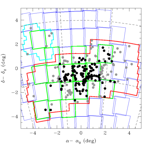
Figure 1: Distribution of the known T2CEPs over the LMC (projected on the sky adopting $\alpha_{0}=81.0$ deg and $\delta_{0}=-69.0$ deg). Grey symbols show all the T2CEPs detected by the OGLE collaboration, whereas black filled circles present the T2CEPs falling in the VMC tiles and studied in this paper. Thin blue and thick green squares (distorted by the projection into the sky) show part of the VMC tiles in the LMC and the 13 tiles treated in this paper, respectively. The thick red and light blue lines show the areas covered by OGLE III and IV (released to date), respectively.

Table 1: Number of T2CEPs in the 13 VMC tiles analysed in this paper, according to OGLE III/IV.

Tile	RA (centre)	DEC (centre)	nT2CEP
LMC	J(2000)	J(2000)
LMC 4_6	05:38:00.41	$-$72:17:20.0	1
LMC 4_8	06:06:32.95	$-$72:08:31.2	2
LMC 5_3	04:58:11.66	$-$70:35:28.0	6
LMC 5_5	05:24:30.34	$-$70:48:34.2	17
LMC 5_7	05:51:04.87	$-$70:47:31.2	4
LMC 6_4	05:12:55.80	$-$69:16:39.4	33
LMC 6_5	05:25:16.27	$-$69:21:08.3	31
LMC 6_6	05:37:40.01	$-$69:22:18.1	20
LMC 6_8	06:02:22.00	$-$69:14:42.4	0
LMC 7_3	05:02:55.20	$-$67:42:14.8	9
LMC 7_5	05:25:58.44	$-$67:53:42.0	6
LMC 7_7	05:49:12.19	$-$67:52:45.5	1
LMC 8_8	05:59:23.14	$-$66:20:28.7	0

2 Type II Cepheids in the VMC survey

T2CEPs in the LMC were identified and studied in the $V,I$ optical bands by Soszyński et al. (2008) in the context of the OGLE III project. We have also considered the recent early release of the OGLE IV survey (Soszyński et al., 2012), including the South Ecliptic Pole (SEP) which, in turn, lies within our tile LMC 8_8. In these surveys, a total of 207 T2CEPs were found (203 by OGLE III and 4 by OGLE IV), of which 65 are BL Her, 98 are W Vir and 44 are RV Tau pulsators.

In this paper we present results for the T2CEPs included on 13 “tiles” (1.5 deg²) completely or nearly completely observed, processed and catalogued by the VMC survey as of March 2013 (and overlapping with the area investigated by OGLE III), namely the tiles LMC 4_6, 4_8, 5_3, 5_5, 5_7, 6_4, 6_5, 6_6, 6_8, 7_3, 7_5, 7_7 and 8_8 (see Fig. 1 and Table 1). Tile LMC 6_6 is centred on the well known 30 Dor star forming region; tiles LMC 5_5, 6_4 and 6_5 are placed on the bar of the LMC. The remaining tiles lie in less crowded regions of the galaxy.

Table 2: Cross-identification and main characteristics of the T2CEPs in the 13 “tiles” analysed in this paper. The columns report: 1) OGLE identification; 2) right ascension (OGLE); 3) declination (OGLE); 4) variability class; 5) intensity-averaged $I$ magnitude (OGLE); 6) intensity-averaged $V$ magnitude (OGLE); 7) period (OGLE); 8) epoch of maximum light $-$2450000 d (OGLE); 9) VMC identification as in the internal VSA release VMC v1.2/v1.3 ( August, 5 2013); 10) VMC Tile; 11) Number of $J$ and $K_{\mathrm{s}}$ epochs, respectively; 12) Notes on individual stars.

ID	RA	DEC	Type	$\langle I\rangle$	$\langle V\rangle$	Period	Epoch	VMC-ID	Tile	NEpochs	Notes
	J2000	J2000		mag	mag	d	d			$J$,$K_{\mathrm{s}}$
(1)	(2)	(3)	(4)	(5)	(6)	(7)	(8)	(9)	(10)	(11)	(12)
OGLE-LMC-T2CEP-123	5:26:19.26	-70:15:34.7	BLHer	18.233	18.723	1.002626	454.80233	558361325273	5_5	4,15	a);b)
OGLE-LMC-T2CEP-069	5:14:56.77	-69:40:22.4	BLHer	18.372	18.919	1.021254	457.21815	558355522273	6_4	4,14	a); b); c)
OGLE-LMC-T2CEP-114	5:23:29.75	-68:19:07.2	BLHer	18.068	19.020	1.091089	2167.44939	558353567228	7_5	4,14	b)
OGLE-LMC-T2CEP-020	4:59:06.12	-67:45:24.6	BLHer	18.036	18.469	1.108126	2166.10854	558351437065	7_3	4,16	a);b)
OGLE-LMC-T2CEP-071	5:15:08.63	-68:54:53.5	BLHer	17.872	18.382	1.152164	457.43379	558354926512	6_4	4,14
OGLE-LMC-T2CEP-089	5:18:35.72	-69:45:45.7	BLHer	18.032	18.492	1.167298	455.65166	558355569068	6_4	11,23
OGLE-LMC-T2CEP-061	5:12:30.42	-69:07:16.2	BLHer	18.018	18.588	1.181512	457.30501	558355098130	6_4	4,14
OGLE-LMC-T2CEP-107	5:22:05.79	-69:40:24.5	BLHer	17.684	18.482	1.209145	455.57377	558356704139	6_5	7,9	d);e)
OGLE-LMC-T2CEP-077	5:16:21.44	-69:36:59.2	BLHer	17.762	18.039	1.213802	456.99603	558355472930	6_4	4,14
OGLE-LMC-T2CEP-165	5:38:15.29	-69:28:57.1	BLHer	18.761	19.723	1.240833	2187.68339	558357659836	6_6	5,14
OGLE-LMC-T2CEP-102	5:21:19.67	-69:56:56.2	BLHer	17.758	18.231	1.266018	455.07285	558356982625	6_5	7,9	d);e)
OGLE-LMC-T2CEP-194	5:57:12.03	-72:17:13.3	BLHer	17.874	18.447	1.314467	2194.11008	558367367174	4_8	5,10
OGLE-LMC-T2CEP-136	5:29:48.11	-69:35:32.1	BLHer	17.823	18.095	1.323038	454.37319	558356602471	6_5	7,9	b)
OGLE-LMC-T2CEP-138	5:30:10.87	-68:49:17.1	BLHer	18.059	18.827	1.393591	2167.52491	558356009909	6_5	7,9	b);d)
OGLE-LMC-T2CEP-109	5:22:12.83	-69:41:50.6	BLHer	19.559	21.212	1.414553	454.69580	558356727002	6_5	7,9	c),d)
OGLE-LMC-T2CEP-105	5:21:58.32	-70:16:35.1	BLHer	17.645	18.206	1.489298	830.77386	558361351217	5_5	4,15
OGLE-LMC-T2CEP-122	5:25:48.19	-68:29:11.4	BLHer	18.241	19.028	1.538669	2167.45087	558353653819	7_5	4,14
OGLE-LMC-T2CEP-171	5:39:40.96	-69:58:01.3	BLHer	17.824	18.512	1.554749	726.82805	558358012379	6_6	5,14
OGLE-LMC-T2CEP-068	5:14:27.05	-68:58:02.0	BLHer	17.671	18.264	1.609301	456.51294	558354968904	6_4	4,14
OGLE-LMC-T2CEP-124	5:26:55.80	-68:51:53.9	BLHer	17.889	18.614	1.734867	2167.63818	558356040530	6_5	7,9
OGLE-LMC-T2CEP-008	4:51:11.51	-69:57:27.0	BLHer	17.842	18.585	1.746099	2165.20369	558358656758	5_3	4,11	c);d);f)
OGLE-LMC-T2CEP-142	5:30:34.92	-68:06:15.2	BLHer	17.580	18.458	1.760753	2167.01120	558353450542	7_5	4,13	a);b);g)
OGLE-LMC-T2CEP-084	5:17:07.50	-69:27:34.1	BLHer	17.512	17.841	1.770840	456.08800	558355348031	6_4	1,8	a);b);g)
OGLE-LMC-T2CEP-141	5:30:23.32	-71:39:00.6	BLHer	17.975	18.757	1.822954	2166.56437	558367767291	4_6	6,14
OGLE-LMC-T2CEP-140	5:30:22.71	-69:15:38.6	BLHer	17.760	18.508	1.841144	2166.65700	558356311759	6_5	7,9
OGLE-LMC-T2CEP-144	5:31:19.82	-68:51:54.9	BLHer	17.750	18.545	1.937450	2166.59387	558356035425	6_5	10,20	a);b);d);f)
OGLE-LMC-T2CEP-130	5:29:04.24	-70:41:37.9	BLHer	17.527	18.124	1.944694	2167.58469	558361658078	5_5	4,15
OGLE-LMC-T2CEP-088	5:18:33.57	-70:50:19.2	BLHer	17.212	17.353	1.950749	2161.24295	558361779217	5_5	4,15	c);d);e)
OGLE-LMC-T2CEP-116	5:23:55.90	-69:25:30.1	BLHer	17.825	18.658	1.966679	445.61278	558356464708	6_5	7,9
OGLE-LMC-T2CEP-121	5:25:42.79	-70:20:46.1	BLHer	17.713	18.430	2.061365	2166.37479	558361402653	5_5	4,15
OGLE-LMC-T2CEP-166	5:38:29.09	-69:45:06.3	BLHer	16.927	17.696	2.110599	2186.16694	558357846207	6_6	5,14	h)
OGLE-LMC-T2CEP-064	5:13:55.87	-68:37:52.1	BLHer	17.514	18.151	2.127891	2167.00843	558354745198	6_4	4,14
OGLE-LMC-T2CEP-167	5:39:02.56	-69:37:38.5	BLHer	17.781	18.597	2.311824	2187.14839	558357756388	6_6	5,14
OGLE-LMC-T2CEP-092	5:19:23.63	-70:02:56.8	BLHer	17.401	18.143	2.616768	2122.71933	558357072491	6_5	8,24
OGLE-LMC-T2CEP-148	5:31:52.26	-69:30:26.4	BLHer	17.442	18.194	2.671734	453.91138	558357678615	6_6	12,23
OGLE-LMC-T2CEP-195	6:02:46.27	-72:12:47.0	BLHer	17.342	18.050	2.752929	2186.99000	558367354217	4_8	5,10
OGLE-LMC-T2CEP-113	5:23:06.33	-69:32:20.5	BLHer	17.137	17.811	3.085460	455.01003	558356568619	6_5	7,9	b);e)
OGLE-LMC-T2CEP-049	5:09:21.88	-69:36:03.0	BLHer	17.130	17.703	3.235275	723.91243	558355501190	6_4	4,14	b)
OGLE-LMC-T2CEP-145	5:31:46.42	-68:58:44.0	BLHer	16.726	17.209	3.337302	2167.28023	558357363019	6_6	12,23
OGLE-LMC-T2CEP-085	5:18:12.87	-71:17:15.4	BLHer	17.142	17.888	3.405095	2160.55457	558362047285	5_5	4,15
OGLE-LMC-T2CEP-030	5:03:35.82	-68:10:16.2	BLHer	16.948	17.755	3.935369	2166.20673	558351663560	7_3	4,16	a);b);g)
OGLE-LMC-T2CEP-134	5:29:28.49	-69:48:00.4	pWVir	16.268	16.851	4.075726	454.54080	558356809300	6_5	7,9
OGLE-LMC-T2CEP-173	5:39:49.93	-69:50:52.9	WVir	18.416	20.149	4.147881	724.81727	558357918488	6_6	5,14	a);b)
OGLE-LMC-T2CEP-120	5:25:29.55	-68:48:11.8	WVir	17.002	17.880	4.559053	2165.73588	558356005996	6_5	7,9
OGLE-LMC-T2CEP-052	5:09:59.34	-69:58:28.7	pWVir	16.395	16.861	4.687925	2164.81082	558355737497	6_4	4,14
OGLE-LMC-T2CEP-098	5:20:25.00	-70:11:08.7	pWVir	14.374	14.671	4.973737	829.46470	558361278143	5_5	4,15
OGLE-LMC-T2CEP-095	5:20:09.84	-68:18:35.3	WVir	17.009	17.873	5.000122	2121.24028	558353571684	7_5	4,14	b);f);g);h)
OGLE-LMC-T2CEP-087	5:18:21.64	-69:40:45.2	WVir	16.887	17.770	5.184979	454.04523	558355510541	6_4	11,23
OGLE-LMC-T2CEP-023	5:00:13.00	-67:42:43.7	pWVir	15.511	16.101	5.234801	2163.87839	558351399660	7_3	4,16
OGLE-LMC-T2CEP-083	5:16:58.99	-69:51:19.3	pWVir	16.531	17.320	5.967650	2119.65683	558355634988	6_4	4,14
OGLE-LMC-T2CEP-062	5:13:19.12	-69:38:57.6	WVir	17.338	18.490	6.046676	453.31305	558355513592	6_4	4,14	b);e)
OGLE-LMC-T2CEP-133	5:29:23.48	-70:24:28.5	WVir	16.671	17.497	6.281955	2162.68787	558361447993	5_5	4,15
OGLE-LMC-T2CEP-137	5:30:03.55	-69:38:02.8	WVir	16.728	17.633	6.362350	453.96088	558356644891	6_5	7,9
OGLE-LMC-T2CEP-183	5:44:32.99	-69:48:21.8	WVir	17.293	18.600	6.509627	2183.46556	558357893157	6_6	5,13
OGLE-LMC-T2CEP-043	5:06:00.44	-69:55:14.6	WVir	16.851	17.774	6.559427	462.41832	558355727258	6_4	4,14	b);f);e);g);h)
OGLE-LMC-T2CEP-159	5:36:42.13	-69:31:11.7	WVir	16.805	17.769	6.625570	2182.53772	558357684253	6_6	5,14
OGLE-LMC-T2CEP-117	5:24:41.50	-71:06:44.6	WVir	16.640	17.539	6.629349	2165.52937	558361934091	5_5	4,15
OGLE-LMC-T2CEP-106	5:22:02.03	-69:27:25.3	WVir	16.612	17.493	6.706736	455.58483	558356498352	6_5	7,9
OGLE-LMC-T2CEP-078	5:16:29.09	-69:24:09.0	pWVir	16.308	17.206	6.716294	455.31768	558355301964	6_4	4,14
OGLE-LMC-T2CEP-063	5:13:43.86	-69:50:41.1	WVir	16.662	17.553	6.924580	2165.50032	558355642907	6_4	4,14
OGLE-LMC-T2CEP-110	5:22:19.48	-68:53:50.0	WVir	16.763	17.705	7.078468	2151.91051	558356071179	6_5	7,9
OGLE-LMC-T2CEP-181	5:43:37.42	-70:38:04.9	pWVir	16.193	16.972	7.212532	724.38026	558360373616	5_7	4,8
OGLE-LMC-T2CEP-047	5:07:46.53	-69:37:00.3	WVir	16.616	17.536	7.286212	723.50042	558355524174	6_4	4,14
OGLE-LMC-T2CEP-056	5:11:19.35	-69:34:32.3	WVir	16.677	17.654	7.289638	452.87968	558355469354	6_4	4,14
OGLE-LMC-T2CEP-100	5:21:14.64	-70:23:15.4	WVir	16.642	17.407	7.431095	825.70218	558361448406	5_5	4,15
OGLE-LMC-T2CEP-111	5:22:22.30	-70:52:46.8	WVir	16.542	17.440	7.495684	829.55773	558361794595	5_5	4,15
OGLE-LMC-T2CEP-170	5:39:38.12	-68:48:24.9	WVir	16.703	-99.990	7.682906	2181.19087	558357268116	6_6	5,14	i)
OGLE-LMC-T2CEP-151	5:34:35.73	-69:59:14.9	WVir	16.479	17.384	7.887246	455.11756	558358035015	6_6	5,14
OGLE-LMC-T2CEP-179	5:43:04.02	-70:01:33.6	WVir	16.744	17.805	8.050065	2185.44813	558358064065	6_6	4,14
OGLE-LMC-T2CEP-182	5:43:46.89	-70:42:36.5	WVir	16.312	17.265	8.226419	2188.39082	558360430553	5_7	4,8
OGLE-LMC-T2CEP-094	5:19:53.20	-69:53:09.9	WVir	16.588	17.529	8.468490	2120.73841	558356923555	6_5	7,9
OGLE-LMC-T2CEP-019	4:58:49.42	-68:04:27.8	pWVir	15.989	16.853	8.674863	2162.74938	558351644677	7_3	4,16
OGLE-LMC-T2CEP-039	5:05:11.31	-67:12:45.3	WVir	16.322	17.192	8.715837	2166.31977	558351083913	7_3	4,16
OGLE-LMC-T2CEP-028	5:03:00.85	-70:07:33.7	pWVir	15.543	16.045	8.784807	2168.94800	558358668771	5_3	4,9
OGLE-LMC-T2CEP-074	5:15:48.75	-68:48:48.1	WVir	16.070	16.892	8.988344	2123.38975	558354851839	6_4	4,14
OGLE-LMC-T2CEP-152	5:34:37.58	-70:01:08.5	WVir	16.453	17.323	9.314921	453.02663	558358053632	6_6	5,14
OGLE-LMC-T2CEP-021	4:59:34.97	-71:15:31.2	pWVir	15.884	16.580	9.759502	2161.10277	558359420632	5_3	4,11
OGLE-LMC-T2CEP-132	5:29:08.23	-69:56:04.3	pWVir	15.818	16.548	10.017829	448.21817	558356939981	6_5	7,9
OGLE-LMC-T2CEP-146	5:31:48.01	-68:49:12.1	WVir	16.392	17.347	10.079593	2161.81703	558357277233	6_6	12,23
OGLE-LMC-T2CEP-097	5:20:20.58	-69:12:20.9	WVir	16.177	17.064	10.510167	446.10816	558356294442	6_5	7,9
OGLE-LMC-T2CEP-022	4:59:58.56	-70:34:27.8	WVir	16.271	17.179	10.716780	2157.78714	558359020369	5_3	4,11
OGLE-LMC-T2CEP-201	5:15:12.67	-69:13:08.0	pWVir	14.611	15.152	11.007243	456.11301	558355159487	6_4	4,14
OGLE-LMC-T2CEP-101	5:21:18.87	-69:11:47.3	WVir	16.035	16.838	11.418560	444.88281	558356283672	6_5	7,9
OGLE-LMC-T2CEP-013	4:55:24.41	-69:55:43.4	WVir	16.184	17.119	11.544611	2157.45185	558358587418	5_3	4,11
OGLE-LMC-T2CEP-178	5:42:19.01	-70:24:08.1	WVir	16.326	17.406	12.212367	726.43160	558360198448	5_7	4,8
OGLE-LMC-T2CEP-127	5:27:59.80	-69:23:27.5	WVir	16.120	17.092	12.669118	454.17111	558356420696	6_5	7,9
OGLE-LMC-T2CEP-118	5:25:15.05	-68:09:11.7	WVir	16.103	17.037	12.698580	2163.34477	558353477576	7_5	4,14
OGLE-LMC-T2CEP-103	5:21:35.27	-70:13:25.7	WVir	16.039	16.995	12.908278	824.38616	558361309970	5_5	4,15
OGLE-LMC-T2CEP-044	5:06:28.86	-69:43:58.8	WVir	16.099	17.108	13.270100	464.57726	558355611443	6_4	4,14
OGLE-LMC-T2CEP-026	5:02:11.56	-68:20:16.0	WVir	16.091	17.026	13.577869	2156.87252	558351786614	7_3	4,16
OGLE-LMC-T2CEP-096	5:20:10.42	-68:48:39.2	WVir	15.918	16.832	13.925722	2129.22374	558356025075	6_5	7,9
OGLE-LMC-T2CEP-157	5:36:02.60	-69:27:16.1	WVir	16.045	17.050	14.334647	2181.19312	558357639701	6_6	5,14
OGLE-LMC-T2CEP-017	4:56:16.02	-68:16:16.4	WVir	15.986	16.968	14.454754	2157.70744	558351791598	7_3	4,16
OGLE-LMC-T2CEP-143	5:31:09.75	-69:15:48.9	WVir	15.806	16.701	14.570185	2166.57316	558356313034	6_5	12,23

Table 3: continued

ID	RA	DEC	Type	$\langle I\rangle$	$\langle V\rangle$	Period	Epoch	VMC-ID	Tile	NEpochs	Notes
	J2000	J2000		mag	mag	d	d
(1)	(2)	(3)	(4)	(5)	(6)	(7)	(8)	(9)	(10)	(11)	(12)
OGLE-LMC-T2CEP-046	5:07:38.94	-68:20:05.9	WVir	15.547	16.415	14.743796	2162.69705	558351740940	7_3	4,16	b);c);d);f)
OGLE-LMC-T2CEP-139	5:30:22.56	-69:09:12.1	WVir	15.968	17.003	14.780410	2156.19900	558356235708	6_5	7,9
OGLE-LMC-T2CEP-177	5:40:36.54	-69:13:04.3	WVir	16.132	17.240	15.035903	2178.31837	558357492207	6_6	5,14
OGLE-LMC-T2CEP-099	5:20:44.48	-69:01:48.4	WVir	15.932	16.999	15.486788	2111.72112	558356167163	6_5	7,9
OGLE-LMC-T2CEP-086	5:18:17.80	-69:43:27.7	WVir	15.629	16.486	15.845500	452.84478	558355544575	6_4	11,23
OGLE-LMC-T2CEP-126	5:27:53.42	-70:51:30.9	WVir	16.210	17.436	16.326778	2167.50661	558361770086	5_5	4,15
OGLE-LMC-T2CEP-057	5:11:21.13	-68:40:13.3	WVir	15.749	16.707	16.632041	2159.16741	558354781673	6_4	4,14
OGLE-LMC-T2CEP-093	5:19:26.45	-69:51:51.0	WVir	15.130	15.861	17.593049	446.06633	558356904142	6_5	7,9	j)
OGLE-LMC-T2CEP-128	5:28:43.81	-70:14:02.3	WVir	15.517	16.460	18.492694	453.20828	558361300181	5_5	4,15
OGLE-LMC-T2CEP-058	5:11:33.52	-68:35:53.7	RVTau	15.511	16.594	21.482951	2167.45398	558354737426	6_4	4,14
OGLE-LMC-T2CEP-104	5:21:49.10	-70:04:34.3	RVTau	14.937	15.830	24.879948	447.75745	558361170450	5_5	11,24
OGLE-LMC-T2CEP-115	5:23:43.53	-69:32:06.8	RVTau	15.593	16.651	24.966913	2145.84889	558356566155	6_5	7,9
OGLE-LMC-T2CEP-192	5:53:55.69	-70:17:11.4	RVTau	15.233	16.148	26.194001	2181.44982	558360150098	5_7	4,8
OGLE-LMC-T2CEP-135	5:29:38.50	-69:15:12.2	RVTau	15.194	16.162	26.522364	2144.30037	558356308540	6_5	7,9
OGLE-LMC-T2CEP-108	5:22:11.27	-68:11:31.3	RVTau	14.746	15.477	30.010843	2113.81336	558353504910	7_5	4,14	k)
OGLE-LMC-T2CEP-162	5:37:44.95	-69:54:16.5	RVTau	15.112	16.200	30.394148	706.20990	558357961649	6_6	5,14
OGLE-LMC-T2CEP-180	5:43:12.87	-68:33:57.1	RVTau	14.502	15.303	30.996315	2178.20791	558352877374	7_7	4,8
OGLE-LMC-T2CEP-119	5:25:19.48	-70:54:10.0	RVTau	14.391	15.225	33.825094	2158.59349	558361803554	5_5	4,15
OGLE-LMC-T2CEP-050	5:09:26.15	-68:50:05.0	RVTau	14.964	15.661	34.748344	713.64755	558354903269	6_4	4,14
OGLE-LMC-T2CEP-200	5:13:56.43	-69:31:58.3	RVTau	15.092	16.124	34.916555	423.70670	558355423319	6_4	4,14	k)
OGLE-LMC-T2CEP-065	5:14:00.75	-68:57:56.8	RVTau	14.699	15.611	35.054940	455.17514	558354970692	6_4	4,14	k)
OGLE-LMC-T2CEP-091	5:18:45.48	-69:03:21.6	RVTau	14.203	14.899	35.749346	425.38622	558355015602	6_4	11,23
OGLE-LMC-T2CEP-203	5:22:33.79	-69:38:08.5	RVTau	15.395	16.723	37.126746	448.74961	558356665485	6_5	7,9
OGLE-LMC-T2CEP-202	5:21:49.09	-70:46:01.4	RVTau	15.167	16.359	38.135567	812.55923	558361722614	5_5	4,15
OGLE-LMC-T2CEP-112	5:22:58.36	-69:26:20.9	RVTau	14.065	14.749	39.397704	421.63429	558356478674	6_5	7,9
OGLE-LMC-T2CEP-051	5:09:41.93	-68:51:25.0	RVTau	14.569	15.440	40.606400	720.05675	558354917278	6_4	4,14	k)
OGLE-LMC-T2CEP-080	5:16:47.43	-69:44:15.1	RVTau	14.341	15.175	40.916413	436.42111	558355560379	6_4	4,14
OGLE-LMC-T2CEP-149	5:32:54.46	-69:35:13.2	RVTau	14.151	14.868	42.480613	2149.99673	558357730269	6_6	5,14
OGLE-LMC-T2CEP-032	5:03:56.31	-67:27:24.6	RVTau	14.011	14.992	44.561195	2152.87623	558351226498	7_3	4,16
OGLE-LMC-T2CEP-147	5:31:51.00	-69:11:46.3	RVTau	13.678	14.391	46.795842	2135.14758	558357481187	6_6	9,23
OGLE-LMC-T2CEP-174	5:40:00.50	-69:42:14.7	RVTau	13.693	14.457	46.818956	2166.79927	558357814883	6_6	5,14
OGLE-LMC-T2CEP-067	5:14:18.11	-69:12:35.0	RVTau	13.825	14.627	48.231705	442.94273	558355160313	6_4	4,14
OGLE-LMC-T2CEP-075	5:16:16.06	-69:43:36.9	RVTau	14.568	15.728	50.186569	430.99079	558355554309	6_4	4,14
OGLE-LMC-T2CEP-014	4:55:35.40	-69:54:04.2	RVTau	14.312	15.103	61.875713	2161.68872	558358564467	5_3	4,11	k)
OGLE-LMC-T2CEP-129	5:28:54.60	-69:52:41.1	RVTau	14.096	14.813	62.508947	397.72780	558356885794	6_5	7,9
OGLE-LMC-T2CEP-045	5:06:34.06	-69:30:03.7	RVTau	13.729	14.787	63.386339	2148.64483	558355447114	6_4	4,14
a) Large separation ($>$ 0.5 arcsec) between VMC and OGLE III star centroids likely due to crowding; b) blended object; c) faint object; d) poor light curve;
e) very low amplitude in the optical; f) source lies within a strip of the tile that has half the exposure of most of the tile (see Cross et al., 2012);
g) poorly sampled or heavily dispersed light curve (due to e.g. blending, saturation); h) source image comes partly from detector 16
(on the top half of detector 16, the quantum efficiency (QE) varies on short timescales making flat-fields inaccurate; Cross et al. 2012);
i) missing OGLE $V$ magnitude; j) light curve showing pulsation plus eclipse according to OGLE III; k) correction for saturation not effective

A detailed description of the general observing strategy of the VMC survey can be found in Cioni et al. (2011). As for the variable stars, the specific procedures adopted to study these objects were discussed in Moretti et al. (2014). Here we only briefly recall that the VMC $K_{\mathrm{s}}$-band time series observations were scheduled in 12 separate epochs distributed over several consecutive months. This strategy allows us to obtain well sampled light curves for a variety of variable types (including RR Lyrae variables and Cepheids of all types). Concerning the $J$ and $Y$ bands, the average number of epochs is 3, as a result of the observing strategy in these bands (i.e. monitoring was not planned). Hence, some epochs could occur in the same night and even one after the other. We note that in this paper we did not consider the $Y$-band data for several reasons: i) this filter is very rarely used in the context of distance scale; ii) its photometric zero point is difficult to calibrate (no 2MASS measures); iii) because the $Y$- band is bluer than the typical NIR bands, the $PL$, $PLC$ and $PW$ relations in this filter are expected to be more dispersed (see e.g. Madore & Freedman, 2012) and of lesser utility with respect to those in $J$ and $K_{\mathrm{s}}$.

The VMC data, processed through the pipeline (Irwin et al., 2004) of the VISTA Data Flow System (VDFS, Emerson et al., 2004) are in the VISTA photometric system (Vegamag=0). The time series photometry used in this paper was retrieved from the VISTA Science Archive (VSA, Cross et al., 2012). For details about the data reduction we refer the reader to the aforementioned papers. Nevertheless, we underline two characteristics of the data reduction which we think may have importance in the subsequent discussion. First, the pipeline is able to correct the photometry of stars close to the saturation limit (Irwin, 2009). This is relevant in the context of this paper because the RV Tau variables discussed here are very bright objects $K_{\mathrm{s}}\sim 12-13$ mag, close to the saturation limits of the VMC survey. The photometry of these stars takes advantage of the VDFS ability to treat saturated images, however, as we will see below, the corrections applied are not always sufficient to fully recover the data. Second, the data retrieved from VSA include quality flags which are very useful to understand if the images have problems. We shall use this information later in this paper.

According to OGLE III/IV, 130 T2CEPs are expected to lie in the 13 tiles analysed in this paper. Note that no T2CEP from OGLE III or OGLE IV falls inside our tiles 6_8 or 8_8, respectively. Hence, in the following we only use OGLE III data. Figure 1 and Table 1 show the distribution of such stars through the VMC tiles.

Table 2 lists the 130 T2CEPs analysed here, together with their main properties as measured by OGLE III and the information about the VMC tile they belong to, as well as the number of epochs of observations in the $J$- and $K_{\mathrm{s}}$-bands. In total, our sample is composed of 41 BL Her, 62 W Vir (12 pW Vir) and 27 RV Tau variables, corresponding to 63%, 63% (75%) and 61% of the known LMC populations of the three different variable classes, respectively.

The OGLE III catalogues of T2CEP variables were cross-correlated against the VMC catalogue to obtain the $J$ and $K_{\mathrm{s}}$ light curves for these variables. All the 130 T2CEPs were found to have a counterpart in the VMC catalogue within 2 arcsec from the OGLE III positions. The great majority of the objects showed separation in position with respect to OGLE III less than 0.1 arcsec. However, 8 stars (OGLE-LMC-T2CEP-020, 030, 069, 084, 123, 142, 144, 173) present separations significantly larger than average ($>$ 0.5 arcsec). Figure 2 shows the OGLE III and VMC finding charts of 29 stars with some kind of identification or data problem, within which we included the eight objects quoted above. It can be seen that all the stars lie in crowded regions or are clearly blended by other stars or diffuse objects (e.g. OGLE-LMC-T2CEP-142). We will discuss these objects further in the following sections.

2.1 T2CEPs light curves

The VMC time series $J$ and $K_{\mathrm{s}}$ photometry for the 130 objects is provided in Table 4, which is published in its entirety in the on-line version of the paper.

Periods and epochs of maximum light available from the OGLE III catalogue were used to fold the $J$- and $K_{\mathrm{s}}$-band light curves produced by the VMC observations. Given the larger number of epochs in $K_{\mathrm{s}}$ with respect to $J$, we discuss first the $K_{\mathrm{s}}$-band data.

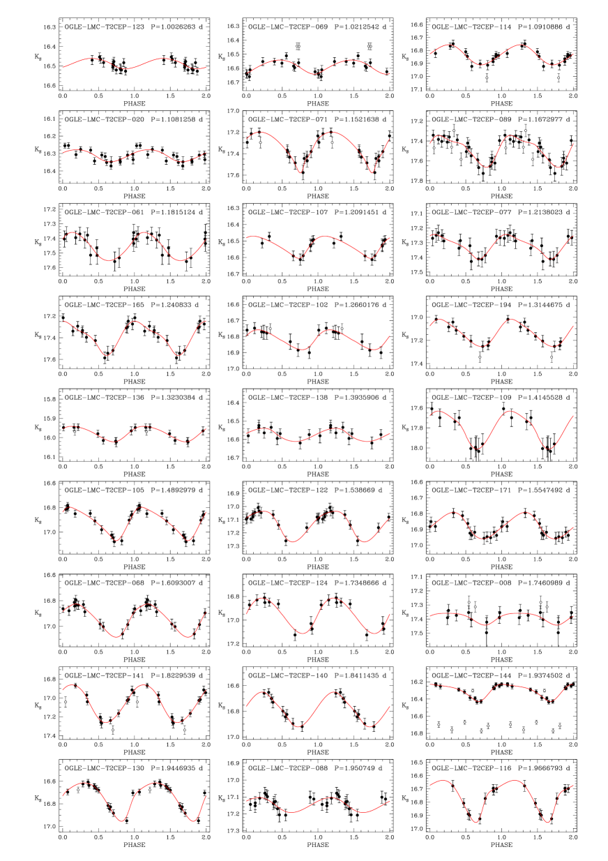
Figure 13: $K_{\mathrm{s}}$-band light curves for T2CEPs with usable data discussed in this paper. Stars are displayed in order of increasing period. Filled and open circles represent phase points used or not used in the fitting procedure, respectively. Solid lines represent best-fitting splines to the data (see text). In each panel we report OGLE’s identification number and period.

The $K_{\mathrm{s}}$–band light curves for a sample of 120 T2CEPs with useful light curves are shown in Fig. 13. Apart from a few cases these light curves are generally well sampled and nicely shaped. Some clearly discrepant data points (empty circles in Fig. 13) in the light curves were excluded from the fit but were plotted in the figure for completeness. Note that most of these “bad” data points belong to observations collected during nights that did not strictly meet the VMC observing constraints (see Table 2 in Cioni et al., 2011). The final spline fit to the data is shown by a solid line in Fig.  13. Intensity-averaged $\langle K_{\mathrm{s}}\rangle$ magnitudes were derived from the light curves using custom software written in C, that performs a spline interpolation to the data with no need of using templates. The numerical model of the light-curve is thus obtained and then integrated in intensity to obtain the mean intensity which is eventually transformed to mean magnitude.

Ten objects in our sample showed unusable light curves, namely: OGLE-LMC-T2CEP-014, 030, 043, 051, 065, 084, 095, 108, 142, 200. Their light curves are displayed in Fig. 18, whereas their finding charts are shown in Fig. 2. A quick analysis of the finding charts reveals that all these stars have significant problems of crowding/blending. Three of the aforementioned objects (OGLE-LMC-T2CEP-030, 084, 142) have centroids significantly shifted with respect to OGLE’s, thus confirming the presence of strong blending.

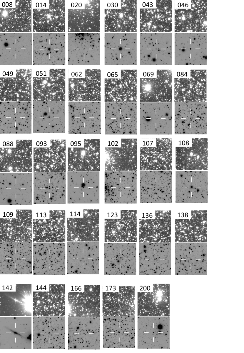
Figure 2: Sky pictures for 29 problematic stars extracted from the VMC (bottom panels) and the OGLE III (top panels) archives. The target is identified with the last three digits of the OGLE III identification (i.e. without the prefix “OGLE-LMC-T2CEP-”).

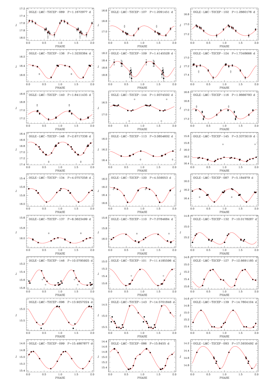
Figure 19: $J$-band light curves for T2CEP stars with a sufficient number of epochs to perform the spline fit to the data. Stars are displayed in order of increasing period. Solid lines represent spline best-fits to the data (see text). In each panel we report OGLE’s identification number and period.

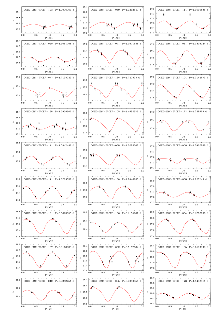
Figure 21: J–band light curves for T2CEP stars not possessing a sufficient number of epochs to perform the spline fit to the data and for which template fitting was used (see text). Stars are displayed in order of increasing period. Solid lines represent spline best-fits to the data (see text). In each panel we report OGLE’s identification number and period.

As for the $J$–band data, Fig. 19 shows the light curves for the 34 stars that have sufficiently good data to allow an independent spline fit (solid line in the figure). Figures 21 and  25 show the light curves for the remaining 86 and 10 objects with small number of epochs ($\sim$4-5 on average) and dispersed light curves, respectively. The latter variables show the same problems reported for the $K_{\mathrm{s}}$-band. To estimate the intensity-averaged $J$ magnitude for the 86 stars possessing only few epochs of observation, we decided to use the spline fit curves in the $K_{\mathrm{s}}$-band as templates. To this aim, for each star we performed the following steps: 1) subtracted the average $\langle K_{\mathrm{s}}\rangle$ magnitude from the $K_{\mathrm{s}}$ spline fit curve; 2) adjusted by eye the data obtained in this way to fit the $J$ light curve by i) adding a zero point; ii) multiplying the amplitude by a proper factor; iii) shifting the light curve in phase. The factor needed for point ii) is the ratio Amp($J$)/Amp($K_{\mathrm{s}}$). To estimate this number, we used the 34 stars with independent $J$–band spline fit, obtaining a value of 1.1$\pm$0.2. The uncertainty of $\sim$20% may appear large, but it does not actually represent a problem since its contribution to the error on the intensity-averaged $J$ is of the order of 0.5%. In some favourable cases, the few data points covered both maximum and minimum of the light curve and it was then possible to constrain directly the amplitude ratio. The shift in phase (point iii above) varied from case to case, but was on average close to 0.05-0.06. The final error on the intensity-averaged $J$ magnitude was calculated by summing in quadrature the error on the $K_{\mathrm{s}}$ magnitude, the uncertainty on the $J$ magnitude caused by the error on the amplitude ratio, and an additional 1% to take into account the uncertainty on the phase shift. The goodness of this procedure can be appreciated in Fig. 3, where we show in different colours the $PL$ and $PW$ relations (see next section for a detailed description of these relations) for the stars with intensity-averaged $J$ photometry obtained directly from spline fits (black points) and with the template fits (grey points). The figure clearly shows that the results obtained on the basis of the $K_{\mathrm{s}}$ templates are usable for scientific purposes. The final $\langle J\rangle$,$\langle K_{\mathrm{s}}\rangle$ magnitudes with relative uncertainties, as well as, pulsational amplitudes and adopted reddening values (see Sect. 3) are provided in Table 5.

Table 4: $J$ and $K_{\mathrm{s}}$ time series photometry for the T2CEPs investigated in this paper. The data below refer to the variable OGLE-LMC-T2CEP-123.

HJD-2 400 000	$J$	$\sigma_{J}$
55487.77111	16.963	0.014
55487.80976	16.959	0.014
55497.79317	16.989	0.014
55497.86048	16.950	0.013
HJD-2 400 000	$K_{\mathrm{s}}$	$\sigma_{K_{\mathrm{s}}}$
55495.82644	16.520	0.020
55497.75937	16.520	0.020
55497.81507	16.513	0.024
55499.82170	16.517	0.023
55511.74774	16.507	0.020
55516.77236	16.496	0.023
55526.78868	16.498	0.021
55539.82483	16.488	0.022
55557.73937	16.482	0.023
55563.71325	16.465	0.021
55587.65755	16.470	0.023
55844.79771	16.526	0.020
55865.82753	16.483	0.021
55887.74744	16.477	0.022
55937.67877	16.454	0.021

Table 4 is published in its entirety only in the electronic edition of the journal. A portion is shown here for guidance regarding its form and content.

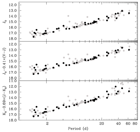
Figure 3: From top to bottom: $PL$ in the $J$ band, $PW$ in ($J$,$V-J$) and $PW$ in ($K_{\mathrm{s}}$,$J-K_{\mathrm{s}}$) for T2CEPs whose intensity-averaged $\langle J\rangle$ magnitude was obtained on the basis of direct spline fit (black filled circles) or template fit (grey filled circles). See the text for details.

We recall that the $J$,$K_{\mathrm{s}}$ photometry presented in this paper is set in the VISTA system. A consistent comparison between our results and those in the widely used 2MASS system (Two Micron All Sky Survey Skrutskie et al., 1996) can be performed after applying proper system transformations as for instance those provided by the Cambridge Astronomy Survey Unit (CASU): ($J$$-$$K_{\mathrm{s}}$)(2MASS)=1.081($J$-$K_{\mathrm{s}}$)(VISTA); $J$(2MASS)=$J$(VISTA)+0.07($J$-$K_{\mathrm{s}}$)(VISTA) and $K_{\mathrm{s}}$(2MASS)=$K_{\mathrm{s}}$(VISTA)$-$0.011($J$-$K_{\mathrm{s}}$)(VISTA).

Since the $\langle$$J$ $\rangle$$-$$\langle$ $K_{\mathrm{s}}$$\rangle$ colour of our T2CEP sample typically ranges from 0.1 to 0.6 mag, the VISTA and 2MASS $K_{\mathrm{s}}$ can be considered equivalent for T2Ceps (see Fig. 4) and for CCs (see Ripepi et al., 2012b), to a very good approximation (better than $\sim$5 mmag).

3 $J$, $K_{\mathrm{s}}$-band Period-Luminosity, Period-Luminosity-Colour and Period-Wesenheit relations

The data reported in Table 5 allow us to calculate different useful relationships adopting various combinations of magnitudes and colours. In particular, we derived $PL$ relations in $J$ and $K_{\mathrm{s}}$ as well as $PW$ and $PLC$ relations for the following combinations: ($J,V-J$); ($K_{\mathrm{s}}$,$V-K_{\mathrm{s}}$); ($K_{\mathrm{s}}$,$J-K_{\mathrm{s}}$).

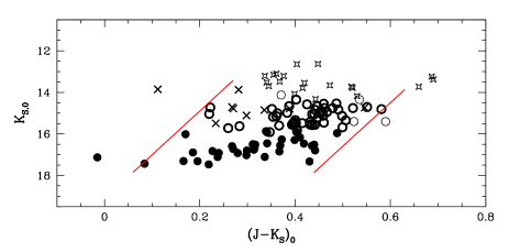
Figure 4: Observed instability strip in the plane $K_{\mathrm{s,0}}$ vs $(J-K_{\mathrm{s}})_{0}$. Filled circles, open circles, crosses and stars show BL Her, W Vir, pW Vir and RV Tau variables, respectively. The solid lines show the approximate borders of the BL Her/W Vir instability strip. Blue and red edges are described by the following equations: $K_{\mathrm{s,0}}$=19.1$-$21$(J-K_{\mathrm{s}})_{0}$ (0.06$<(J-K_{\mathrm{s}})_{0}<$0.27 mag) and $K_{\mathrm{s,0}}$=27.1$-$21$(J-K_{\mathrm{s}})_{0}$ (0.44$<(J-K_{\mathrm{s}})_{0}<$0.63 mag), respectively.

We first corrected magnitudes and colours for reddening using the recent extinction maps by Haschke, Grebel & Duffau (2011). Individual $E$($V$$-$$I$) reddening values for the 120 T2CEPs with useful VMC data are reported in column 10 of Table 5. The reliability of this reddening correction can be questioned by observing that it has been derived from the analysis of the Red Clump (RC) stars, which trace the intermediate-age population (2-9 Gyr) instead of the old one to whom BL Her and W Vir belong to. However, we recall that in the NIR bands the interstellar absorption is very low: $A_{J}\sim 0.25A_{V}$ and $A_{K_{\mathrm{s}}}\sim 0.1A_{V}$, where $A_{V}$ is the absorption in the visible. Hence, even in the unlikely case of a 10% large error in our $A_{V}$ estimates, this would introduce an amount of uncertainties of only $\sim$2.5% and $\sim$1% in $J$ and $K_{\mathrm{s}}$, respectively. An a posteriori indication about the global correctness of the adopted reddening correction is represented by the concordance of results provided by the $PL$ (reddening dependent) and $PW$ (reddening independent) relations (see Sect. 4 and  5). The reddening values were converted using the following equations: $E$($V$$-$$J$)=1.80$E$($V$$-$$I$); $E$($V$$-$$K_{\mathrm{s}}$)=2.24$E$($V$$-$$I$) $E$($J$$-$$K_{\mathrm{s}}$)=0.43$E$($V$$-$$I$) (Cardelli, Clayton, & Mathis, 1989; Gao et al., 2013). The coefficients of the $PW$ relations were calculated in a similar way.

Table 5: Results for the 120 T2CEPs with useful NIR light curves analysed in this paper. The columns report: 1) OGLE identification; 2) variability class ; 3) period (OGLE); 4) intensity–averaged $J$ magnitude; 5) uncertainty on the $\langle J\rangle$ 6) intensity–averaged $K_{\mathrm{s}}$ magnitude; 7) uncertainty on the $\langle K_{\mathrm{s}}\rangle$; 8) peak–to–peak amplitude in $J$; 9) peak–to–peak amplitude in $K_{\mathrm{s}}$; 10) adopted reddening; 11) T=results in $J$ obtained on the basis of the $K_{\mathrm{s}}$ template, S=results in $J$ obtained on the basis of direct spline fitting to the data.

ID	Var. Class	Period	$\langle J\rangle$	$\sigma_{\langle J\rangle}$	$\langle K_{\mathrm{s}}\rangle$	$\sigma_{\langle K_{\mathrm{s}}\rangle}$	$Amp(J)$	$Amp(K_{\mathrm{s}})$	$E($V-I$)$	Note
		d	mag	mag	mag	mag	mag	mag	mag
(1)	(2)	(3)	(4)	(5)	(6)	(7)	(8)	(9)	(10)	(11)
OGLE-LMC-T2CEP-123	BLHer	1.0026263	16.939	0.021	16.486	0.013	0.05	0.05	0.080	T
OGLE-LMC-T2CEP-069	BLHer	1.0212542	17.042	0.033	16.585	0.021	0.10	0.10	0.050	T
OGLE-LMC-T2CEP-114	BLHer	1.0910886	17.329	0.069	16.831	0.019	0.17	0.16	0.130	T
OGLE-LMC-T2CEP-020	BLHer	1.1081258	16.735	0.043	16.310	0.022	0.09	0.07	0.060	T
OGLE-LMC-T2CEP-071	BLHer	1.1521638	17.522	0.022	17.326	0.026	0.40	0.38	0.070	T
OGLE-LMC-T2CEP-089	BLHer	1.1672977	17.715	0.018	17.479	0.043	0.40	0.32	0.040	S
OGLE-LMC-T2CEP-061	BLHer	1.1815124	17.581	0.037	17.458	0.031	0.38	0.19	0.090	T
OGLE-LMC-T2CEP-107	BLHer	1.2091451	16.979	0.005	16.526	0.016	0.19	0.13	0.030	S
OGLE-LMC-T2CEP-077	BLHer	1.2138023	17.521	0.045	17.317	0.025	0.18	0.17	0.020	T
OGLE-LMC-T2CEP-165	BLHer	1.2408330	17.889	0.049	17.381	0.024	0.34	0.32	0.180	T
OGLE-LMC-T2CEP-102	BLHer	1.2660176	17.146	0.010	16.817	0.020	0.20	0.13	0.070	S
OGLE-LMC-T2CEP-194	BLHer	1.3144675	17.406	0.017	17.134	0.018	0.38	0.24	0.080	T
OGLE-LMC-T2CEP-136	BLHer	1.3230384	16.492	0.011	15.978	0.006	0.31	0.08	0.060	S
OGLE-LMC-T2CEP-138	BLHer	1.3935906	16.975	0.043	16.576	0.017	0.07	0.07	0.070	T
OGLE-LMC-T2CEP-109	BLHer	1.4145528	18.610	0.056	17.790	0.038	0.43	0.38	0.030	S
OGLE-LMC-T2CEP-105	BLHer	1.4892979	17.134	0.012	16.914	0.021	0.41	0.27	0.080	T
OGLE-LMC-T2CEP-122	BLHer	1.5386690	17.520	0.034	17.136	0.018	0.24	0.23	0.110	T
OGLE-LMC-T2CEP-171	BLHer	1.5547492	17.175	0.017	16.875	0.017	0.18	0.17	0.170	T
OGLE-LMC-T2CEP-068	BLHer	1.6093007	17.225	0.028	16.942	0.018	0.27	0.26	0.100	T
OGLE-LMC-T2CEP-124	BLHer	1.7348666	17.280	0.009	16.953	0.030	0.30	0.30	0.110	S
OGLE-LMC-T2CEP-008	BLHer	1.7460989	17.257	0.023	17.389	0.028	0.08	0.08	0.100	T
OGLE-LMC-T2CEP-141	BLHer	1.8229539	17.389	0.023	17.048	0.021	0.36	0.40	0.100	T
OGLE-LMC-T2CEP-140	BLHer	1.8411435	17.127	0.012	16.779	0.014	0.21	0.27	0.080	S
OGLE-LMC-T2CEP-144	BLHer	1.9374502	16.726	0.017	16.302	0.011	0.22	0.20	0.120	S
OGLE-LMC-T2CEP-130	BLHer	1.9446935	17.036	0.016	16.740	0.021	0.36	0.34	0.060	T
OGLE-LMC-T2CEP-088	BLHer	1.9507490	17.158	0.012	17.147	0.028	0.09	0.09	0.060	T
OGLE-LMC-T2CEP-116	BLHer	1.9666793	17.086	0.038	16.746	0.007	0.23	0.32	0.060	S
OGLE-LMC-T2CEP-121	BLHer	2.0613655	17.234	0.033	16.854	0.014	0.45	0.43	0.030	T
OGLE-LMC-T2CEP-166	BLHer	2.1105987	16.343	0.015	15.922	0.006	0.23	0.22	0.190	T
OGLE-LMC-T2CEP-064	BLHer	2.1278906	17.043	0.019	16.698	0.025	0.47	0.45	0.070	T
OGLE-LMC-T2CEP-167	BLHer	2.3118238	17.091	0.045	16.685	0.010	0.50	0.48	0.320	T
OGLE-LMC-T2CEP-092	BLHer	2.6167684	16.864	0.097	16.526	0.066	0.69	0.66	0.050	T
OGLE-LMC-T2CEP-148	BLHer	2.6717338	16.853	0.011	16.516	0.015	0.43	0.56	0.060	S
OGLE-LMC-T2CEP-195	BLHer	2.7529292	16.850	0.021	16.474	0.008	0.55	0.46	0.080	T
OGLE-LMC-T2CEP-113	BLHer	3.0854602	16.285	0.002	15.935	0.008	0.10	0.06	0.020	S
OGLE-LMC-T2CEP-049	BLHer	3.2352751	16.359	0.015	15.926	0.010	0.25	0.24	0.070	T
OGLE-LMC-T2CEP-145	BLHer	3.3373019	16.269	0.008	16.047	0.015	0.11	0.08	0.120	S
OGLE-LMC-T2CEP-085	BLHer	3.4050955	16.640	0.017	16.191	0.011	0.47	0.45	0.090	T
OGLE-LMC-T2CEP-134	pWVir	4.0757258	15.782	0.009	15.514	0.007	0.31	0.36	0.080	S
OGLE-LMC-T2CEP-173	WVir	4.1478811	16.049	0.018	15.452	0.005	0.12	0.11	0.170	T
OGLE-LMC-T2CEP-120	WVir	4.5590530	16.354	0.007	15.951	0.009	0.38	0.38	0.130	S
OGLE-LMC-T2CEP-052	pWVir	4.6879253	16.031	0.018	15.741	0.022	0.14	0.13	0.070	T
OGLE-LMC-T2CEP-098	pWVir	4.9737372	14.056	0.014	13.892	0.005	0.15	0.14	0.120	T
OGLE-LMC-T2CEP-087	WVir	5.1849790	16.302	0.013	15.859	0.015	0.30	0.31	0.090	S
OGLE-LMC-T2CEP-023	pWVir	5.2348007	15.005	0.043	14.720	0.013	0.36	0.34	0.040	T
OGLE-LMC-T2CEP-083	pWVir	5.9676496	15.936	0.054	15.462	0.011	0.48	0.46	0.100	T
OGLE-LMC-T2CEP-062	WVir	6.0466764	16.060	0.019	15.431	0.003	0.05	0.05	0.090	T
OGLE-LMC-T2CEP-133	WVir	6.2819551	16.013	0.010	15.564	0.013	0.09	0.09	0.040	T
OGLE-LMC-T2CEP-137	WVir	6.3623499	16.044	0.004	15.630	0.010	0.11	0.11	0.110	S
OGLE-LMC-T2CEP-183	WVir	6.5096275	16.325	0.016	15.739	0.016	0.15	0.14	0.200	T
OGLE-LMC-T2CEP-159	WVir	6.6255696	16.089	0.015	15.605	0.010	0.09	0.09	0.110	T
OGLE-LMC-T2CEP-117	WVir	6.6293487	16.007	0.012	15.579	0.005	0.12	0.11	0.080	T
OGLE-LMC-T2CEP-106	WVir	6.7067363	15.956	0.055	15.474	0.010	0.16	0.15	0.050	T
OGLE-LMC-T2CEP-078	pWVir	6.7162943	15.349	0.016	14.764	0.011	0.15	0.14	0.090	T
OGLE-LMC-T2CEP-063	WVir	6.9245800	16.040	0.023	15.577	0.016	0.14	0.13	0.050	T
OGLE-LMC-T2CEP-110	WVir	7.0784684	15.978	0.008	15.511	0.017	0.16	0.15	0.120	S
OGLE-LMC-T2CEP-181	pWVir	7.2125323	15.505	0.013	15.151	0.005	0.07	0.07	0.130	T
OGLE-LMC-T2CEP-047	WVir	7.2862123	15.943	0.018	15.511	0.011	0.14	0.13	0.070	T
OGLE-LMC-T2CEP-056	WVir	7.2896382	15.965	0.017	15.522	0.004	0.16	0.15	0.110	T
OGLE-LMC-T2CEP-100	WVir	7.4310950	15.965	0.012	15.647	0.020	0.29	0.28	0.080	T
OGLE-LMC-T2CEP-111	WVir	7.4956838	15.865	0.011	15.441	0.006	0.19	0.18	0.060	T
OGLE-LMC-T2CEP-170	WVir	7.6829062	15.926	0.018	15.423	0.004	0.16	0.15	0.180	T
OGLE-LMC-T2CEP-151	WVir	7.8872458	15.814	0.016	15.366	0.009	0.14	0.13	0.110	T
OGLE-LMC-T2CEP-179	WVir	8.0500650	15.932	0.014	15.378	0.005	0.14	0.13	0.110	T
OGLE-LMC-T2CEP-182	WVir	8.2264194	15.628	0.035	15.218	0.007	0.37	0.35	0.130	T
OGLE-LMC-T2CEP-094	WVir	8.4684897	15.659	0.048	15.143	0.006	0.10	0.10	0.040	T
OGLE-LMC-T2CEP-019	pWVir	8.6748634	15.263	0.024	14.880	0.015	0.33	0.31	0.110	T
OGLE-LMC-T2CEP-039	WVir	8.7158373	15.682	0.018	15.217	0.009	0.19	0.18	0.040	T
OGLE-LMC-T2CEP-028	pWVir	8.7848073	15.083	0.016	14.791	0.006	0.32	0.30	0.050	T
OGLE-LMC-T2CEP-074	WVir	8.9883439	15.414	0.019	15.025	0.025	0.22	0.21	0.060	T
OGLE-LMC-T2CEP-152	WVir	9.3149211	15.559	0.013	15.080	0.004	0.39	0.37	0.100	T
OGLE-LMC-T2CEP-021	pWVir	9.7595024	15.309	0.046	15.059	0.018	0.16	0.15	0.070	T
OGLE-LMC-T2CEP-132	pWVir	10.0178287	15.227	0.015	14.804	0.005	0.22	0.09	0.080	S
OGLE-LMC-T2CEP-146	WVir	10.0795925	15.576	0.026	15.172	0.021	0.37	0.29	0.100	S
OGLE-LMC-T2CEP-097	WVir	10.5101666	15.530	0.062	15.068	0.006	0.28	0.27	0.050	T
OGLE-LMC-T2CEP-022	WVir	10.7167800	15.598	0.011	15.126	0.015	0.35	0.33	0.030	T
OGLE-LMC-T2CEP-201	pWVir	11.0072431	14.195	0.018	13.892	0.007	0.06	0.06	0.050	T
OGLE-LMC-T2CEP-101	WVir	11.4185596	15.427	0.009	15.009	0.007	0.45	0.40	0.080	S
OGLE-LMC-T2CEP-013	WVir	11.5446113	15.498	0.014	15.001	0.013	0.22	0.21	0.090	T
OGLE-LMC-T2CEP-178	WVir	12.2123667	15.517	0.020	14.985	0.008	0.33	0.31	0.150	T
OGLE-LMC-T2CEP-127	WVir	12.6691185	15.372	0.022	14.851	0.011	0.48	0.37	0.070	S
OGLE-LMC-T2CEP-118	WVir	12.6985804	15.412	0.038	14.914	0.007	0.72	0.69	0.100	T
OGLE-LMC-T2CEP-103	WVir	12.9082775	15.336	0.011	14.859	0.019	0.40	0.38	0.080	T
OGLE-LMC-T2CEP-044	WVir	13.2701004	15.455	0.030	14.835	0.013	0.30	0.29	0.090	T
OGLE-LMC-T2CEP-026	WVir	13.5778689	15.209	0.089	14.823	0.012	0.39	0.37	0.080	T
OGLE-LMC-T2CEP-096	WVir	13.9257224	15.277	0.056	14.776	0.006	0.81	0.75	0.090	S
OGLE-LMC-T2CEP-157	WVir	14.3346466	15.304	0.045	14.782	0.043	0.66	0.63	0.100	T
OGLE-LMC-T2CEP-017	WVir	14.4547544	15.354	0.056	14.785	0.021	0.81	0.77	0.110	T
OGLE-LMC-T2CEP-143	WVir	14.5701846	14.991	0.075	14.743	0.068	1.05	0.72	0.060	S

Table 6: continued

ID	Var. Class	Period	$\langle J\rangle$	$\sigma_{\langle J\rangle}$	$\langle K_{\mathrm{s}}\rangle$	$\sigma_{\langle K_{\mathrm{s}}\rangle}$	$Amp(J)$	$Amp(K_{\mathrm{s}})$	$E($V-I$)$	Note
		d	mag	mag	mag	mag	mag	mag	mag
(1)	(2)	(3)	(4)	(5)	(6)	(7)	(8)	(9)	(10)	(11)
OGLE-LMC-T2CEP-046	WVir	14.7437956	14.921	0.058	14.360	0.021	0.62	0.59	0.060	T
OGLE-LMC-T2CEP-139	WVir	14.7804104	15.220	0.014	14.709	0.005	0.50	0.51	0.150	S
OGLE-LMC-T2CEP-177	WVir	15.0359027	15.245	0.024	14.741	0.007	0.69	0.66	0.270	T
OGLE-LMC-T2CEP-099	WVir	15.4867877	15.094	0.003	14.564	0.005	0.51	0.52	0.100	S
OGLE-LMC-T2CEP-086	WVir	15.8455000	15.024	0.011	14.586	0.017	0.79	0.80	0.030	S
OGLE-LMC-T2CEP-126	WVir	16.3267785	15.323	0.023	14.733	0.013	0.77	0.73	0.090	T
OGLE-LMC-T2CEP-057	WVir	16.6320415	15.052	0.021	14.566	0.013	0.82	0.78	0.060	T
OGLE-LMC-T2CEP-093	WVir	17.5930492	14.524	0.021	14.136	0.019	0.61	0.47	0.040	S
OGLE-LMC-T2CEP-128	WVir	18.4926938	14.787	0.023	14.363	0.054	0.71	0.68	0.050	T
OGLE-LMC-T2CEP-058	RVTau	21.4829509	14.777	0.017	14.208	0.014	0.75	0.71	0.090	T
OGLE-LMC-T2CEP-104	RVTau	24.8799480	14.131	0.020	13.402	0.043	0.32	0.61	0.090	S
OGLE-LMC-T2CEP-115	RVTau	24.9669126	14.790	0.002	14.334	0.013	0.66	0.63	0.030	S
OGLE-LMC-T2CEP-192	RVTau	26.1940011	14.521	0.033	14.096	0.008	1.09	1.04	0.060	T
OGLE-LMC-T2CEP-135	RVTau	26.5223638	14.350	0.016	13.799	0.015	1.09	0.76	0.070	S
OGLE-LMC-T2CEP-162	RVTau	30.3941483	14.294	0.043	13.726	0.043	0.57	0.41	0.220	T
OGLE-LMC-T2CEP-180	RVTau	30.9963145	13.785	0.068	12.921	0.033	0.42	0.40	0.070	T
OGLE-LMC-T2CEP-119	RVTau	33.8250938	13.832	0.021	12.951	0.064	0.89	0.85	0.080	T
OGLE-LMC-T2CEP-050	RVTau	34.7483438	14.257	0.030	13.811	0.014	0.19	0.18	0.070	T
OGLE-LMC-T2CEP-091	RVTau	35.7493456	13.652	0.045	12.693	0.055	0.62	0.64	0.070	S
OGLE-LMC-T2CEP-203	RVTau	37.1267463	14.416	0.007	13.739	0.004	0.61	0.39	0.040	S
OGLE-LMC-T2CEP-202	RVTau	38.1355674	14.310	0.013	13.753	0.015	0.07	0.07	0.090	T
OGLE-LMC-T2CEP-112	RVTau	39.3977037	13.531	0.021	13.163	0.009	0.27	0.24	0.030	S
OGLE-LMC-T2CEP-080	RVTau	40.9164131	13.957	0.027	13.253	0.047	0.44	0.42	0.040	T
OGLE-LMC-T2CEP-149	RVTau	42.4806129	13.649	0.039	13.252	0.007	0.13	0.12	0.140	T
OGLE-LMC-T2CEP-032	RVTau	44.5611948	13.232	0.030	12.212	0.090	0.36	0.34	0.050	T
OGLE-LMC-T2CEP-147	RVTau	46.7958419	13.145	0.017	12.658	0.013	0.06	0.06	0.090	T
OGLE-LMC-T2CEP-174	RVTau	46.8189562	13.089	0.016	12.048	0.030	0.46	0.44	0.150	T
OGLE-LMC-T2CEP-067	RVTau	48.2317051	13.176	0.022	12.263	0.052	0.20	0.19	0.100	T
OGLE-LMC-T2CEP-075	RVTau	50.1865686	13.900	0.110	13.502	0.033	0.78	0.74	0.070	T
OGLE-LMC-T2CEP-129	RVTau	62.5089466	13.514	0.035	13.123	0.013	0.16	0.14	0.070	S
OGLE-LMC-T2CEP-045	RVTau	63.3863391	13.098	0.024	12.664	0.021	0.16	0.15	0.070	T

In principle, an additional preliminary step would be required, i.e. the correction for the inclination of the LMC disc-like structure by de-projecting each T2CEP with respect to the LMC centre. To do this we followed the procedure suggested in van der Marel & Cioni (2001) and adopted their values of the LMC centre, inclination, and position angle of the line of nodes. However, we have a posteriori verified that the introduction of this correction leads to worse results, i.e. larger dispersion in the various relationships mentioned above. To verify if different choices about the inclined disc parameters could improve the results, we have carried out the de-projection using several results present in the literature (see Haschke et al., 2012; Rubele et al., 2012; Subramanian & Subramaniam, 2013, and references therein). Under no circumstances the dispersion of the $PWs$ decreased (we used $PWs$ as reference because they are reddening-free). To explain this occurrence we can reasonably hypothesise that the T2CEPs (actually BL Her and W Vir), being old (age$>$ 10 Gyr) objects, are not preferentially distributed along the main disc-like structure of the LMC. Alternatively, the adopted parameters for the de-projection are not accurate enough, although this conclusion may be influenced by the relatively small number of objects. Subsequent studies using a larger number of objects observed in the VMC context sampling different populations (CCs, T2CEPs, RR Lyrae stars) will clarify the issue. In any case, in the following analysis we did not apply any magnitude correction accounting for the LMC disk structure.

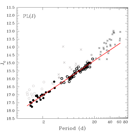
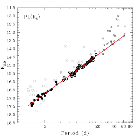
Figure 5: $PL(J)$ and $PL(K_{\mathrm{s}})$ relations for the T2CEPs investigated in this paper. The meaning of the symbols is the following: black filled and empty circles are the BL Her and W Vir variables used in the derivation of the $PL$, $PW$ and $PLC$ relationships, respectively. Grey empty and filled circles are the BL Her and W Vir variables discarded because of problems in the photometry (see text). Grey crosses are the peculiar W Vir stars. The starred symbols represent the RV Tau variables. The size of the symbols is generally representative of the measurement errors. The solid lines represent the least-squares fit to the data shown in Table 7. We recall that RV Tau stars were not used in the calculation of the least-squares fits (see text).

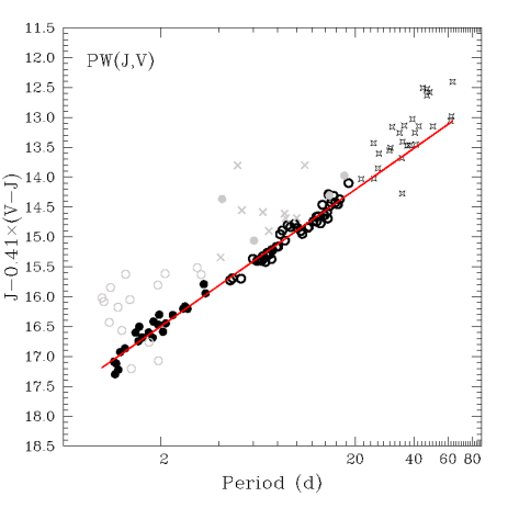
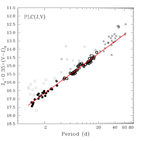
Figure 6: $PW(J,V)$ and $PLC(J,V)$ for the T2CEPs investigated in this paper. Symbols are as in Fig. 5.

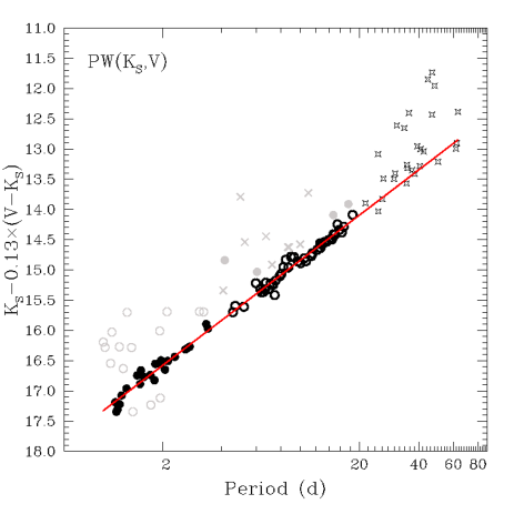
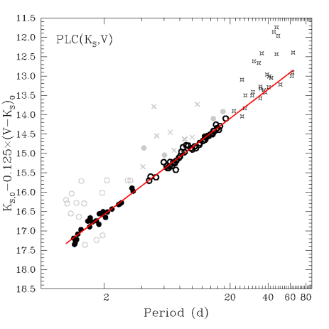
Figure 7: $PW(K_{\mathrm{s}},V)$ and $PLC(K_{\mathrm{s}},V)$ for the T2CEPs investigated in this paper. Symbols are as in Fig. 5.

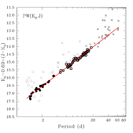
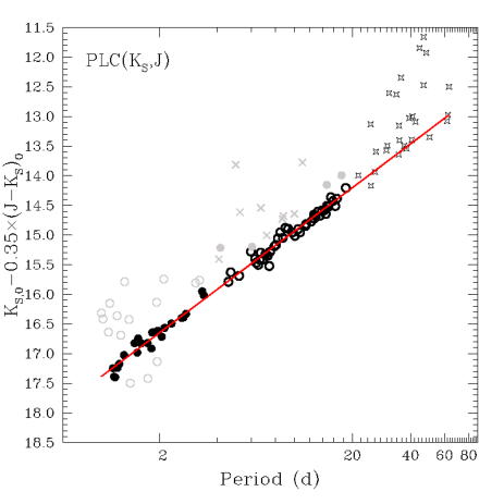
Figure 8: $PW(K_{\mathrm{s}},J)$ and $PLC(K_{\mathrm{s}},J)$ for the T2CEPs investigated in this paper. Symbols are as in Fig. 5.

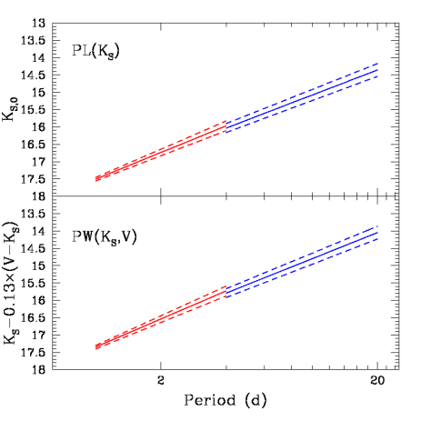
Figure 9: Top panel: $PL(K_{\mathrm{s}})$ relation calculated separately for for BL Her (red) and W Vir (blue) variables. The solid and dashed lines show the best-fit $\pm$1 $\sigma$ error (both for slope and $ZP$), respectively. Bottom panel: as above but for the $PW(K_{\mathrm{s}},J-K_{\mathrm{s}})$ relation.

Figures 5, 6, 7 and  8 show all the relationships investigated here. An inspection of these figures confirms the findings by Matsunaga, Feast, & Menzies (2009) that BL Her and W Vir star follow a common $PL$ relation, whereas RV Tau show a different and more dispersed relation (the dispersion is less severe in the $J$ than in the $K_{\mathrm{s}}$-band). In our case the dispersion among RV Tau stars can in part be due to the proximity of several bright variables to the saturation limit. As a consequence, we decided to exclude these stars from the calculation of the $PL$, $PW$ and $PLC$ relations. To check if BL Her and W Vir stars can actually be fitted with an unique relation we performed an independent test by fitting separately the $PL(K_{\mathrm{s}},J)$ and $PW(K_{\mathrm{s}},V)$ relations for each class of variables. The result of this exercise is shown in Fig. 9: for both relations, the two variable classes seem to show results that agree with each other well within 1 $\sigma$, thus confirming that we can use BL Her and W Vir variables together.

For each combination of periods, magnitudes and colours, we performed independent least-squares fits to the data, adopting equations of the form reported in Table 7. The results of the fitting procedure are shown in the same table as well as in Figures 5, 6, 7 and  8 with a solid line. Note that the equations listed in Table 7 are given in terms of absolute magnitudes since we subtracted the dereddened distance modulus ($DM_{0,LMC}$) of the LMC from each equation. Thus, the absolute zero point (ZP) of the relations in Table 7 can be simply obtained by using the preferred value for the $DM_{0,LMC}$ value.

In deriving the equations of Table 7, we have implicitly neglected any dependence of both $PL$ and $PW$ relations on the metallicity of the pulsators. This is in agreement with Matsunaga et al. (2006), who found a hardly significant dependence of the $PL$ relations on metallicity (0.1$\pm$0.06 mag/dex), whereas the theoretical models by Di Criscienzo et al. (2007) predict a very mild metallicity dependence $\Delta$Mag/$\Delta$ [Fe/H]$\sim 0.04-0.06$ mag/dex for both the $PL$ and $PW$ relations in the magnitudes and colours of interest. In any case, the very low dispersions of our $PL$ and $PW$ relations listed in Table 7, seems to suggest that the metallicity dependence, if any, should be very small. Alternatively, a small dispersion in metallicity among our sample could explain the results as well. However, since the low metallicity dependence found by Matsunaga et al. (2006) is based on T2CEPs spanning a wide range of [Fe/H], the latter explanation is less likely.

Table 7: Relevant relationships derived in this work. Note that all the results are in the VISTA photometric system. $DM_{LMC,0}$ stands for the LMC dereddened distance modulus.

method	Relation	$r.m.s$ (mag)
$PL(J)$	$M_{J,0}=(-2.19\pm 0.04)\log P+(17.700\pm 0.035)-DM_{LMC,0}$	0.13
$PL(K_{\mathrm{s}})$	$M_{K_{\mathrm{s,0}}}=(-2.385\pm 0.03)\log P+(17.47\pm 0.02)-DM_{LMC,0}$	0.09
$PW(J,V)$	$M_{J}-0.41(V-J)=(-2.290\pm 0.035)\log P+(17.19\pm 0.03)-DM_{LMC,0}$	0.11
$PLC(J,V)$	$M_{J,0}=(-2.40\pm 0.05)\log P+(0.35\pm 0.07)(V-J)_{0}+(17.385\pm 0.065)-DM_{LMC,0}$	0.11
$PW(K_{\mathrm{s}},V)$	$M_{K_{\mathrm{s}}}-0.13(V-K_{\mathrm{s}})=(-2.49\pm 0.03)\log P+(17.33\pm 0.02)-DM_{LMC,0}$	0.08
$PLC(K_{\mathrm{s}},V)$	$M_{K_{\mathrm{s,0}}}=(-2.48\pm 0.04)\log P+(0.125\pm 0.040)(V-K_{\mathrm{s}})_{0}+(17.33\pm 0.05)-DM_{LMC,0}$	0.08
$PW(K_{\mathrm{s}},J)$	$M_{K_{\mathrm{s}}}-0.69(J-K_{\mathrm{s}})=(-2.52\pm 0.03)\log P+(17.320\pm 0.025)-DM_{LMC,0}$	0.085
$PLC(K_{\mathrm{s}},J)$	$M_{K_{\mathrm{s,0}}}=(-2.45\pm 0.04)\log P+(0.35\pm 0.14)(J-K_{\mathrm{s}})_{0}+(17.39\pm 0.04)-DM_{LMC,0}$	0.085

In each figure, a number of stars are shown with grey symbols. They significantly deviate from almost all relationships discussed above. The crosses represent the stars classified by Soszyński et al. (2008) as peculiar W Vir (see column 4 in Table 2), i.e. suspected binaries that do not follow the optical $PL$ and $PW$ relations. We note that three of these peculiar W Vir stars, namely OGLE-LMC-T2CEP-021, 052 and 083 do not show any difference with respect to the normal W Vir stars in our $PL$, $PW$ and $PLC$ planes, and were hence included in the calculations. As for BL Her and W Vir, 15 and 4 stars of the two classes were not used in the least-squares fits because, with few exceptions, they show large scattering in almost all the relationships calculated here, and, in particular in the most reliable ones, namely the $PWs$ and $PLCs$ based on the $K_{\mathrm{s}}$-band photometry. The finding charts for all these stars are displayed in Fig. 2, whereas the notes in Table 2 explain in detail the causes that led us to exclude these objects, with blending by close companions being the most common cause.

Table 7 deserves some discussion: i) the dispersion of the $PL(J)$ relation is, as expected, larger than for the $PL(K_{\mathrm{s}})$; ii) for any combination of magnitude and colour, the dispersions of $PW$ and $PLC$ are equal (this reflects the correctness of the reddening correction applied in this paper); iii) the $PW(J,V)$ and $PLC(J,V)$ are significantly more dispersed than the $PW(K_{\mathrm{s}},V)$-$PLC(K_{\mathrm{s}},V)$ and $PW(K_{\mathrm{s}},J)$-$PLC(K_{\mathrm{s}},J)$ couples; iv) the best combination of magnitude and colour (lower dispersion) appears to be the $K_{\mathrm{s}}$,$V$; v) the color coefficients of the $PW(K_{\mathrm{s}},V)$ and $PLC(K_{\mathrm{s}},V)$ relations are very similar and the two relations are coincident. Similarly, for $PW(J,V)$ and $PLC(J,V)$ the colour coefficients are the same within the errors, whereas this is not true for the couple $PW(K_{\mathrm{s}},J)$; $PLC(K_{\mathrm{s}},J)$.

Table 8: $PL(K_{\mathrm{s}})$ and $PW(K_{\mathrm{s}})$ relations for LMC T2CEPs with the $ZP$ calibrated as follows: (2) by imposing a $DM_{LMC,0}$=18.46$\pm$0.03 mag (from CCs in the LMC Ripepi et al., 2012b) in Table 7; (3) by adopting Galactic T2CEP ($\kappa$ Pav) and RR Lyrae variables with $HST$ parallaxes (Benedict et al., 2011) and T2CEPs with BW distance estimates (Feast et al., 2008); (4) by adopting only calibrators with the quoted $HST$ parallaxes. See text for additional details.

Relation	$ZP_{CC}$	$ZP_{\pi+BW}$	$ZP_{\pi}$
(1)	(2)	(3)	(4)
$K_{\mathrm{s,0}}=(-2.385\pm 0.03)\log P+ZP$	$-0.99\pm 0.04$	$-1.09\pm 0.10$	$-1.11\pm 0.10$
$K_{\mathrm{s}}-0.13(V-K_{\mathrm{s}})=(-2.49\pm 0.03)\log P+ZP$	$-1.13\pm 0.04$	$-1.24\pm 0.10$	$-1.26\pm 0.10$

4 Absolute calibration of $PL$, $PLC$ and $PW$ relations

In Table 7 we provided the absolute $ZP$ for the relevant $PL$, $PLC$ and $PW$ relations as a function of the $DM_{0,LMC}$. However, it is of considerable astrophysical interest to obtain an independent absolute calibration for at least some of these relations. Indeed, this would allow us to obtain an independent measure of the distance to the LMC and to the GGCs hosting T2CEP variables. To this aim, we can only rely on calibrators located close enough to the Sun to have a measurable parallax or whose distances have been estimated by Baade-Wesselink (BW) techniques (see Gautschy, 1987, for a review on this method). There are only two T2CEPs whose parallaxes were measured with reasonable accuracy with the $Hubble~{}Space~{}Telescope$ ($HST$; Benedict et al., 2011), namely $\kappa$ Pav (W Vir) and VY Pyx (BL Her). For two additional BL Her variables, SW Tau and V533 Cen, as well as for $\kappa$ Pav, a BW-based distance is also available (Feast et al., 2008). However, VY Pyx turned out to be a peculiar star, unusable as calibrator (see discussion in Benedict et al., 2011). As for $\kappa$ Pav, the pulsational parallax estimated by Feast et al. (2008) through BW analysis is about 2$\sigma$ smaller than the trigonometric parallax measured by $HST$ and adopted here ($\Delta\pi=0.67\pm 0.33$ mas). Feast et al. (2008) investigated the possible causes of the discrepancy with respect to the Hipparcos parallax (van Leeuwen, 2007), which was even larger than the $HST$ one, but did not find any definitive explanation. A well known potential problem related with the application of the BW technique is the uncertainty on the projection factor p (see, e.g. Molinaro et al., 2012; Nardetto et al., 2014, and references therein). In their analysis Feast et al. (2008) derived and adopted a fixed p-factor = 1.23$\pm$ 0.03. However, several researchers suggested that the p-factor actually does depend on the period of the pulsator (see e.g. Barnes, 2009; Laney & Joner, 2009; Storm et al., 2011a; Nardetto et al., 2014, and references therein), hence, for example, different p-factor values should be used for BL Her and W Wir stars. Given the uncertainties on the projection factor discussed above, in the following we will adopt the $HST$-based distance for $\kappa$ Pav, and the zero point of the different $PL,PW$ and $PLC$ relations will be estimated including or not the BW-based distances for SW Tau and V533 Cen. Finally, we note that $[Fe/H]$($\kappa$ Pav)$\approx$+0.0 dex (Feast et al., 2008), i.e. at least 1 dex more metal rich than expected for typical T2CEPs. Hence, some additional uncertainty when using this object as a distance indicator can be caused by a possible metallicity effect. However, as discussed in Sect. 3, the metal dependence of the T2CEP $PLs$, if any, should be very small, and we do not expect the high metallicity of $\kappa$ Pav to be an issue for our purposes. To enlarge the number of reliable calibrators, a possibility is to use the 5 RR Lyrae stars whose parallax were measured with $HST$ by Benedict et al. (2011). Indeed, as already hypothesised by Sollima, Cacciari, & Valenti (2006) and Feast et al. (2008), RR Lyrae and T2CEPs follow the same $PL(K_{\mathrm{s}})$ relation (Caputo et al., 2004, found similar results in the optical bands). To further test this possibility, we draw in Fig. 10 the $PL(K_{\mathrm{s}})$ and $PW(K_{\mathrm{s}})$ relations for the T2CEPs analysed in this paper, in comparison with the location occupied in the same planes by the RR Lyrae stars in the LMC (light blue filled circles, after Borissova et al., 2009). The periods of c-type RR Lyrae stars were fundamentalised by adding $\delta$logP=0.127 (Bono et al., 1997a) and the magnitudes have been corrected for the metallicity term devised by Sollima, Cacciari, & Valenti (2006), using the individual metallicity measurement compiled by Borissova et al. (2009). It can be seen that both the $PL(K_{\mathrm{s}})$ and $PW(K_{\mathrm{s}})$ relations (red lines) derived for T2CEPs in Sect. 5 tightly match the location of the RR Lyrae stars. On this basis, we decided to proceed using also the RR Lyrae with $HST$ parallax to anchor the $ZP$ of the $PL(K_{\mathrm{s}})$ and $PW(K_{\mathrm{s}},V)$ relations for T2CEPs. To this aim, we simply adopted the slopes of the quoted relations from Table 7, corrected for metallicity the $ZP$ for the five RR Lyrae stars with $HST$ parallaxes and calculated the weighted average of the results in two cases: i) including only stars with $HST$parallax, namely, $\kappa$ Pav and the five RR Lyrae stars; ii) using the stars at point i) plus the two T2CEPs with BW analysis, namely SW Tau and V533 Cen. The results of these procedures are outlined in Table 8 (columns 3 and 4) and in Fig. 11. For comparison, column (2) of Table 8 shows the $ZPs$ obtained assuming $DM_{0,LMC}=18.46\pm 0.03$ mag, as derived by Ripepi et al. (2012b) from LMC CC stars. We choose the work by Ripepi et al. (2012b) as reference for CCs because: i) these Authors adopted a procedure similar to the one adopted in this work; ii) their results are in excellent agreement with the most recent and accurate literature findings (see e.g. Storm et al., 2011b; Joner & Laney, 2012; Laney, Joner, & Pietrzyński, 2012; Walker, 2012; Pietrzyński et al., 2013; de Grijs, Wicker, & Bono, 2014, and references therein) An analysis of Table 8 reveals that: i) the inclusion of the two stars with BW-based distances does not change significantly the $ZPs$ and ii) there is a difference of at least $\sim$0.1 mag between the $ZPs$ calibrated on the basis of CCs and of Galactic T2CEPs (see Sect. 5).

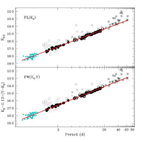
Figure 10: $PL(K_{\mathrm{s}})$ and $PW(K_{\mathrm{s}},V)$ relations for the T2CEPs analysed in this paper (symbols as in Fig. 5) and for the sample of RR Lyrae stars in the LMC observed by Borissova et al. (2009) (light blue filled circles). The red lines show the relationships listed in Table 7 extended till the periods of the RR Lyrae stars.

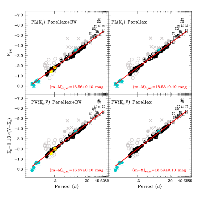
Figure 11: Absolute $PL(K_{\mathrm{s}})$ and $PW(K_{\mathrm{s}},V)$ relations for the T2CEPs analysed in this paper (symbols as in Fig. 5). Light blue and yellow filled circles show the objects whose distances were measured through $HST$ parallaxes (Benedict et al., 2011) or through BW analysis (Feast et al., 2008), respectively. The red line shows the best-fit line to the data adopting the slope from Table 7, while $ZPs$ were calculated using the objects with $HST$ parallaxes alone (right panels), and by adding to them the objects with BW analysis (left panels). The true $DMs$ estimated in each case for the LMC are also labelled (see Sect. 5).

4.1 Comparison with the literature

The relationships presented in Tables 7 and  8 can now be compared to those available in the literature. As mentioned in the introduction, Matsunaga et al. (2006) and Matsunaga, Feast, & Menzies (2009) published the $PL$ relations in the $JHK_{\mathrm{s}}$ bands for BL Her and W Vir variables hosted by GGCs and the LMC, respectively. These results can be compared with ours, provided that we first transform all the $J$ and $K_{\mathrm{s}}$ magnitudes into the VISTA system. With this aim, we transformed the Matsunaga et al. (2006) photometry from 2MASS to VISTA using the equations reported in Sect. 2.1. The results of Matsunaga, Feast, & Menzies (2009) are in the IRSF system, whose $J$ and $K_{\mathrm{s}}$ can in principle be transformed to the 2MASS system (Kato et al., 2007), and in turn, into the VISTA system. However, this is not possible for the $J$ band, because we lack $H$-band photometry (see Table 10 in Kato et al., 2007). We can safely overcome this problem by noting that the $(J-H)$ colour for BL Her and W Vir stars spans a very narrow range (0.25$<(J-H)<$0.4 mag, see e.g. Matsunaga, Feast, & Soszyński, 2011) so that, according to Kato et al. (2007) we can assume $J$(IRSF)=$J$(2MASS)+(0.005$\pm$0.005). Finally, since our targets span the range 0.25$<(J-K_{\mathrm{s}})<$0.6 mag, we obtained: $J$(IRSF)=$J$(VISTA)+(0.035$\pm$0.015). As for the $K_{\mathrm{s}}$, the transformation is straightforward: $K_{\mathrm{s}}$(IRSF)=$K_{\mathrm{s}}$(VISTA)+(0.014$\pm$0.001).

The $PL$ relations by Matsunaga et al. (2006) and Matsunaga, Feast, & Menzies (2009), corrected as discussed above, are presented in the first four rows of Table 9. We can compare directly the $PL(J)$ and $PL(K_{\mathrm{s}})$ relations for the LMC (lines 2 and 4 in Table 9) with our results (lines 1 and 2 in Table 7). There is a very good agreement within 1 $\sigma$ errors for the $PL(J)$, whereas for the $PL(K_{\mathrm{s}})$ the comparison is slightly worse, especially concerning the slope of the relation which is discrepant at the 1.5$\sigma$ level. It is also worth mentioning that the dispersion of our relations is significantly smaller, as a result of the much better light curve sampling of the VMC data.

Table 9: Values for the coefficients of the $PL$, $PW$ and $PLC$ relations for BL Her and W Vir Cepheids taken from the literature. The $PW$ functions are defined as in Table 7. The errors of $ZP$ take into account the uncertainties in the transformation of the $J$ and $K_{\mathrm{s}}$ photometry to the VISTA system (see text for details).

method	Relation	$\sigma$ (mag)
Results by Matsunaga et al. (2006) and Matsunaga, Feast, & Menzies (2009) transformed to the VISTA system
$PL(J)$ GCs	$M_{J,0}=(-2.23\pm 0.05)\log P-(0.84\pm 0.03)$	0.16
$PL(J)$ LMC	$J_{0}=(-2.16\pm 0.04)\log P+(17.76\pm 0.03)$	0.21
$PL(K_{\mathrm{s}})$ GCs	$M_{K_{\mathrm{s,0}}}=(-2.41\pm 0.05)\log P-(1.11\pm 0.03)$	0.14
$PL(K_{\mathrm{s}})$ LMC	$K_{\mathrm{s,0}}=(-2.28\pm 0.05)\log P+(17.40\pm 0.03)$	0.21
Results by Di Criscienzo et al. (2007) transformed to the VISTA system
$PL(J)$	$M_{J,0}=(-2.29\pm 0.04)\log P-(0.73\pm 0.13)$
$PL(K_{\mathrm{s}})$	$M_{K_{\mathrm{s,0}}}=(-2.38\pm 0.02)\log P-(1.10\pm 0.07)$
$PW(J,V)$	$M_{J}-0.41(V-J)=(-2.37\pm 0.02)\log P-(1.15\pm 0.08)$
$PW(K_{\mathrm{s}},V)$	$M_{K_{\mathrm{s}}}-0.13(V-K_{\mathrm{s}})=(-2.52\pm 0.02)\log P-(1.25\pm 0.08)$
$PW(K_{\mathrm{s}},J)$	$K_{\mathrm{s}}-0.69(J-K_{\mathrm{s}})=(-2.60\pm 0.02)\log P-(1.27\pm 0.08)$

As for the $PL(J)$ and $PL(K_{\mathrm{s}})$ derived for GGCs by Matsunaga et al. (2006), their slopes are in very good agreement with ours, which suggest a “universal slope” in the NIR filters, independent of the galactic environment. As for the $ZPs$, we can only compare them for the $PL(K_{\mathrm{s}})$ relations (see Table 8). We found an excellent agreement when the $ZP$ is calibrated through the Galactic calibrators (irrespectively of whether stars with BW measures are included or not), whereas there is a 0.12 mag discrepancy if the $ZP$ is calibrated by means of the LMC $DM$ coming from CCs. This occurrence is not surprising, since Matsunaga et al. (2006) used the $M_{V}$ vs $[Fe/H]$ relation for RR Lyrae variables by Gratton et al. (2003) to estimate the distances of the GGCs hosting T2CEPs and derive their $PL(K_{\mathrm{s}})$. Hence, the two population II calibrators, RR Lyrae and T2CEPs, give distance scales in agreement with each other.

A similar comparison can be performed with the theoretical predictions by Di Criscienzo et al. (2007), who in addition calculated the $PWs$ for all the combinations of magnitudes and colours of interest in this work. Again, we converted the Di Criscienzo et al. (2007) results from the Bessell & Brett (1988) (BB) to the VISTA system. To do this, we used the transformations BB-2MASS from Carpenter (2001) and 2MASS-VISTA (see Section 2.1) and the same procedure as above to derive: $J$(BB)=$J$(VISTA)+(0.04$\pm$0.010); $K_{\mathrm{s}}$(BB)=$K_{\mathrm{s}}$(VISTA)+(0.030$\pm$0.015). Secondly, since the predicted $PL$ and $PW$ relations mildly depend on metallicity and adopted a mixing length parameter ($\alpha$), we have to make a choice for these parameters. We decided to evaluate the relations for $\alpha$=1.5$\pm$0.5 (to encompass reasonable values for $\alpha$) and [Fe/H]=$-1.5\pm$0.3 dex as an average value for the LMC old population (see, e.g. Borissova et al., 2004, 2006; Gratton et al., 2004; Haschke et al., 2012). The uncertainties on these parameters were taken into account in re-deriving the $ZP$ of the predicted $PL$ and $PW$ relations in the VISTA system. The result of this procedure is shown in the second part of Table 9. A comparison with Table 8 shows that both for the $PL(K_{\mathrm{s}})$ and $PW(K_{\mathrm{s}},V)$ relations there is an excellent agreement between ours and theoretical results if the quoted relationships are calibrated with the Galactic T2CEPs and RR lyrae, whereas there is a $\sim$0.1 mag discrepancy if we adopt the CC-based $DM$ by Ripepi et al. (2012b) for the LMC to define the $ZP$. However, if we take into account the uncertainties this discrepancy results formally not significant within 1$\sigma$.

5 Discussion

The results reported in Sect. 4 allow us to discuss the distance of the LMC as estimated from NIR observation of the T2CEPs hosted in this galaxy. Table 10 (columns 3 and 4) lists the $DM_{0,LMC}$ calculated using the different $ZP$ estimates for the $PL(K_{\mathrm{s}})$ and $PW(K_{\mathrm{s}},V)$ relations listed in Table 8. An inspection of the table reveals that the $DM_{0,LMC}$ calculated by means of CCs (column 2 in Table 10) and by means of the T2CEPs differ by more than $\sim$0.1 mag, even if, formally there is agreement within 1 $\sigma$. Since both the Ripepi et al. (2012b) calibration for CCs and that presented here for T2CEPs are based on a weighted mix of $HST$ parallaxes and BW analysis, this discrepancy, albeit only partially significant, seems to suggest that the distance scales calibrated on pulsating stars belonging to population I and population II give different results (for a recent comprehensive review of the literature and a discussion about this argument, see de Grijs, Wicker, & Bono, 2014).

An additional application of the absolute $PL(K_{\mathrm{s}})$ relation for T2CEPs concerns the distance estimate of GGCs hosting such kind of pulsators. Homogeneous $K_{\mathrm{s}}$ photometry, as well as period of pulsation for most of the known T2CEPs in GGCs were published by Matsunaga et al. (2006) (see their Table 2). We simply inserted the period of these variables in the $PL(K_{\mathrm{s}})$ of Table 8, and by difference with the observed magnitudes, we derived the $DM$ for each GGC. When more than one T2CEP was present in a cluster, we averaged the resulting $DMs$ (we excluded from the calculations the variables with periods longer than about 35 d because they are likely neither BL Her nor W Vir variables). The result of such a procedure is shown in Fig. 12 where for each GGC analysed here, we show (as a function of the metal content of the clusters) the difference between the $DMs$ estimated on the basis of the three different calibration of the $PL(K_{\mathrm{s}})$ listed in Table 8 and the $DMs$ reported by Harris (1996) in his catalogue of GGCs parameters. In Fig. 12 the average discrepancy in $DMs$ decreases from top to bottom, suggesting that, even if the statistical significance is low (due to the large dispersion in $\Delta DM$ values $\sim$ 0.14 mag), the distance scale of GGCs, if estimated on the basis of the T2CEPs hosted in this systems, is more consistent with population II rather than population I standard candles. This is not particularly surprising since most of the distances of GGCs in the Harris catalogue are based on RR Lyrae stars.

Table 10: $DM$ of the LMC estimated on the basis of the different $PL(K_{\mathrm{s}})$ and $PW(K_{\mathrm{s}})$ relations described in Table 8 (see text).

Relation	$DM^{LMC}_{CC}$	$DM^{LMC}_{\pi+BW}$	$DM^{LMC}_{\pi}$
(1)	(2)	(3)	(4)
$PL(K_{\mathrm{s}})$	$18.46\pm 0.04$	$18.56\pm 0.10$	$18.58\pm 0.10$
$PW(K_{\mathrm{s}},V)$	$18.46\pm 0.04$	$18.57\pm 0.10$	$18.59\pm 0.10$

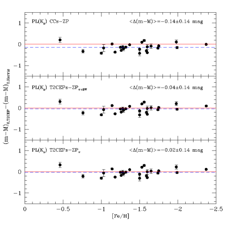
Figure 12: Distance modulus differences (this work-Harris 1996) for a sample of GGCs hosting T2CEPs as a function of [Fe/H]. The dashed blue line shows the average difference. The solid red line show the line with zero difference. The $DMs$ for the GGCs were estimated adopting the $PL(K_{\mathrm{s}})$ for T2CEPs and $ZP$ determined as follows: (top panel) on the basis of the $DM_{0,LMC}$ measured by Ripepi et al. (2012b) using LMC CC with VMC NIR data; (middle panel) by means of a sample of Galactic T2CEPs whose distances were measured both through $HST$ parallaxes (Benedict et al., 2011) and BW technique (Feast et al., 2008); (bottom panel) as in the previous case, but using objects with $HST$ parallaxes only.

6 Summary

In the context of the VMC survey, this paper shows the first results concerning type II Cepheids in the LMC. We presented $J$ and $K_{\mathrm{s}}$ light curves for 130 pulsators, including 41 BL Her, 62 W Vir (12 pW Vir) and 27 RV Tau variables, corresponding to 63%, 63% (75%) and 61% of the known LMC populations of the three variable classes, respectively. The $K_{\mathrm{s}}$ band light curves are almost always well sampled, allowing us to obtain accurate spline fits to the data and, in turn, precise intensity-averaged $\langle K_{\mathrm{s}}\rangle$ magnitudes for 120 variables in our sample. As for the $J$ band, only about 1/3 of the $J$ light curves were sufficiently sampled to allow a satisfactory spline fit to the data, for the remaining 2/3 of pulsators, the intensity-averaged $\langle J\rangle$ magnitudes were derived using the $K_{\mathrm{s}}$ band spline fits as templates. On the basis of this data set for BL Her and W Vir, complemented by the $\langle V\rangle$ magnitudes from the OGLE survey, we have built for the first time (apart from $PL(J)$ and $PL(K_{\mathrm{s}})$) a variety of empirical $PL$, $PLC$ and $PW$ relationships, for any combination of the $V,J,K_{\mathrm{s}}$ filters. Several outliers were removed from the calculation of these relations, and we provided an explanation for the presence of these divergent objects. All the quoted $PL$, $PLC$ and $PW$ relationships were calibrated in terms of the LMC distance. However, the availability of absolute $M_{V}$ and $M_{K_{\mathrm{s}}}$ for a small sample of RR Lyrae and T2CEPs variables based on $HST$ parallaxes allowed us to obtain an independent absolute calibration of the $PL(K_{\mathrm{s}})$ and $PW(K_{\mathrm{s}},V)$ relationships (the $PLC(K_{\mathrm{s}},V)$ is identical to the $PW(K_{\mathrm{s}},V)$). If applied to the LMC and to the GGCs hosting T2CEPs, these relations give distance moduli which are around 0.1 mag longer than those estimated for Classical Cepheids by means of $HST$ parallaxes and BW techniques. However, if we take into account the uncertainties at their face value, the quoted discrepancy is formally not significant within 1$\sigma$.

Appendix A Light Curves

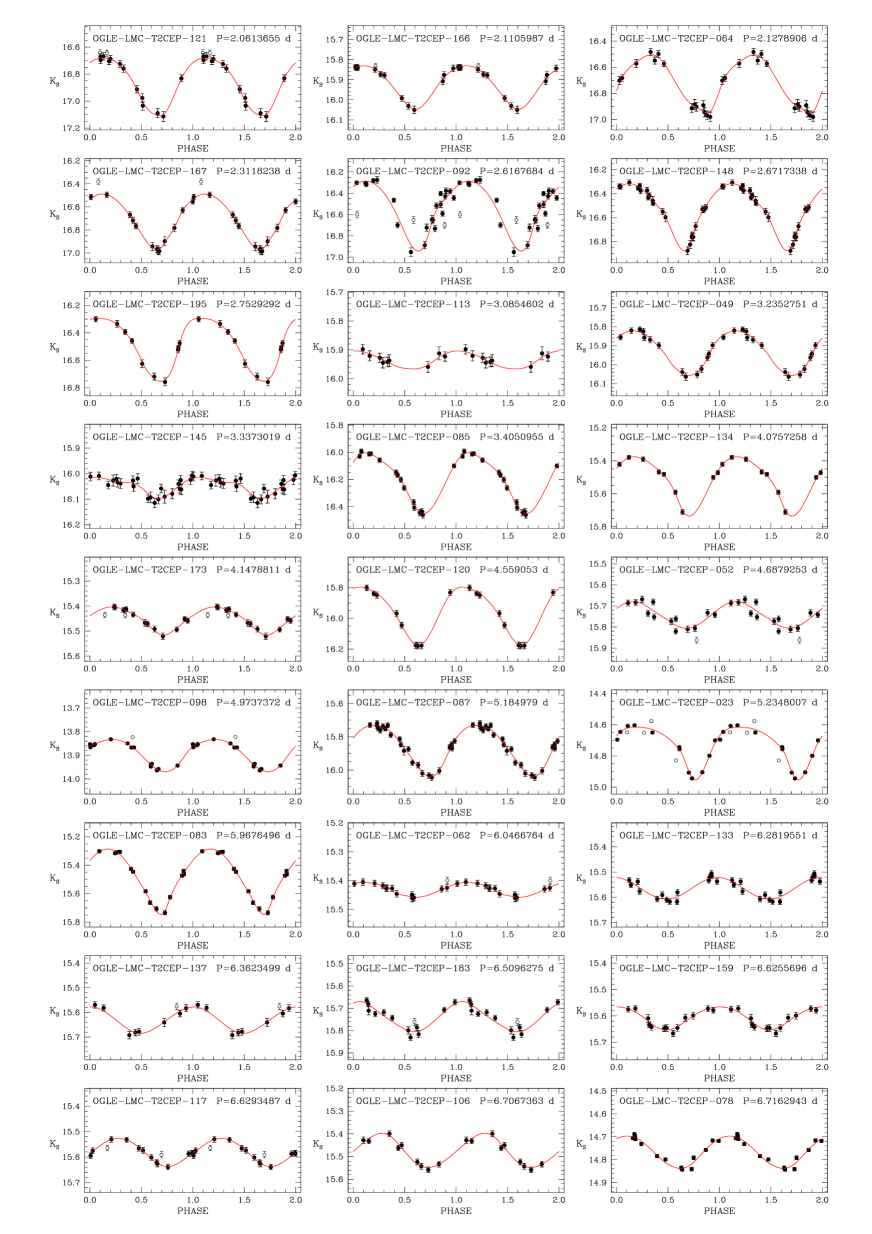
Figure 14: continued

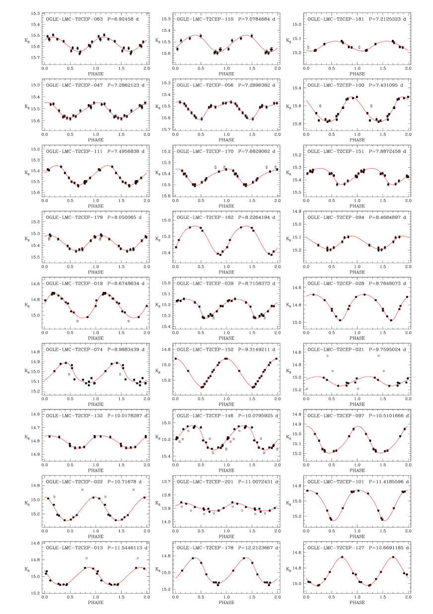
Figure 15: continued

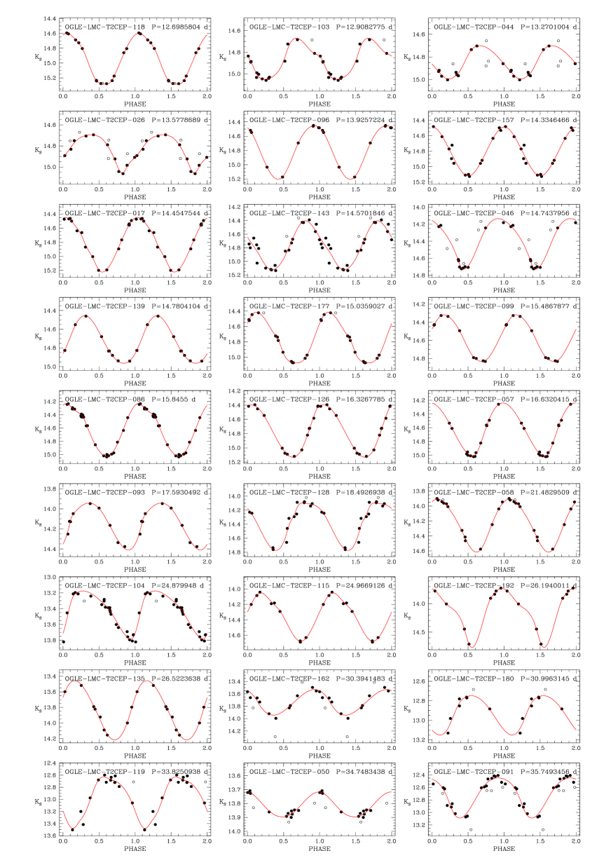
Figure 16: continued

Figure 17: continued

Figure 18: $K_{\mathrm{s}}$–band light curves for problematic stars (see text).

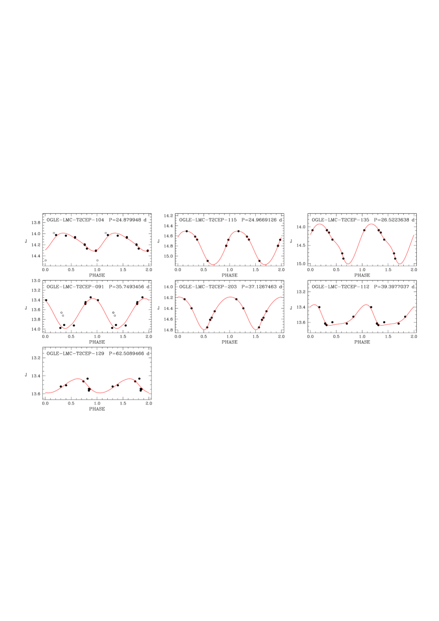
Figure 20: continued

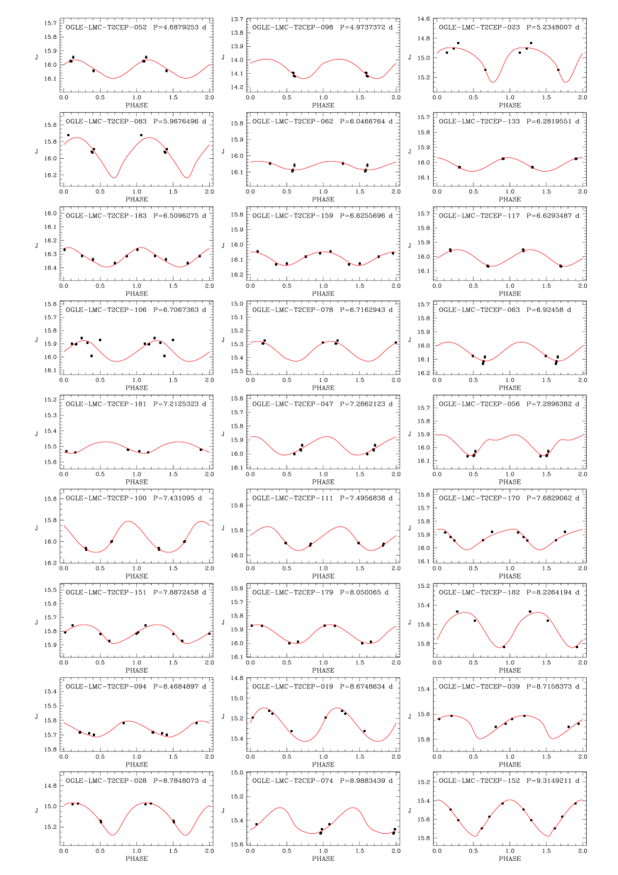
Figure 22: continued

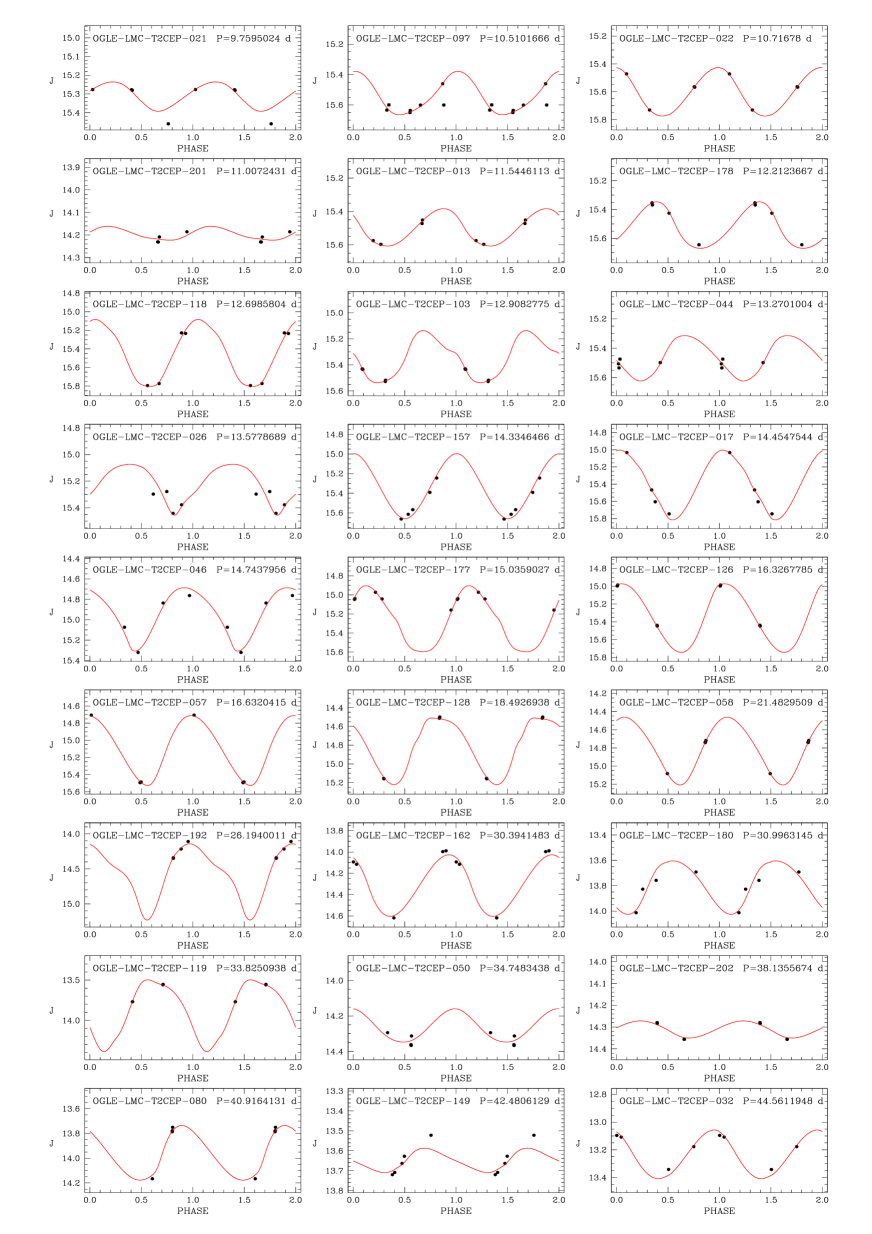
Figure 23: continued

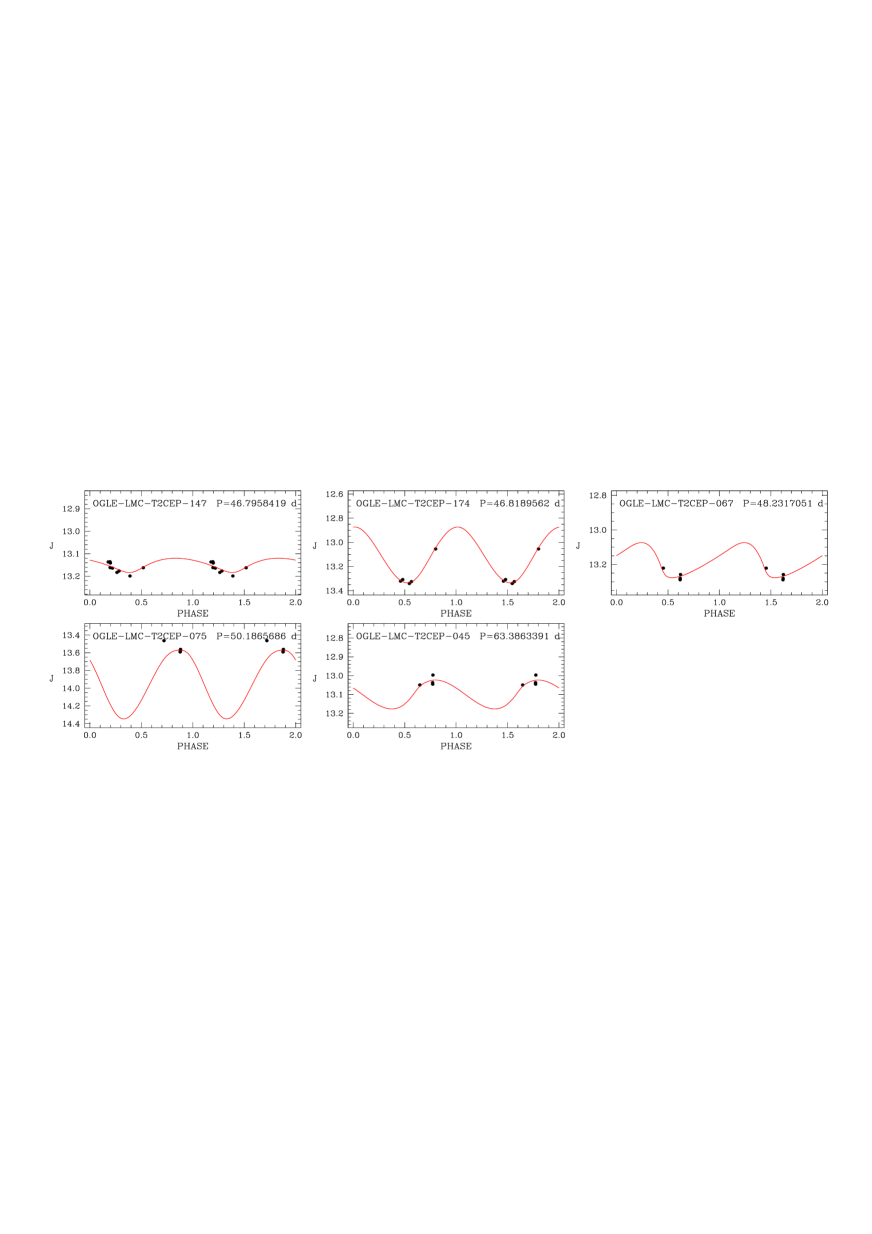
Figure 24: continued

Figure 25: Light curves for stars showing problems in the $J$- and $K_{\mathrm{s}}$-band (see text).

References

- Barnes (2009) Barnes T. G., 2009, AIPC, 1170, 3
- Bekki & Chiba (2007) Bekki K., Chiba M., 2007, MNRAS, 381, L16
- Benedict et al. (2011) Benedict G. F., et al., 2011, AJ, 142, 187
- Bessell & Brett (1988) Bessell, M. S., Brett, J. M., 1988, PASP, 100, 1134
- Bono et al. (1997a) Bono G., Caputo F., Castellani V., Marconi M., 1997a, A&AS, 121, 327
- Bono, Caputo, & Santolamazza (1997b) Bono G., Caputo F., Santolamazza P., 1997b, A&A, 317, 171
- Borissova et al. (2004) Borissova J., Minniti D., Rejkuba M., Alves D., Cook K. H., Freeman K. C., 2004, A&A, 423, 97
- Borissova et al. (2006) Borissova J., Minniti D., Rejkuba M., Alves D., 2006, A&A, 460, 459
- Borissova et al. (2009) Borissova J., Rejkuba M., Minniti D., Catelan M., Ivanov V. D., 2009, A&A, 502, 505
- Brocato et al. (2004) Brocato E., Caputo F., Castellani V., Marconi M., Musella I., 2004, AJ, 128, 1597
- Caputo (1998) Caputo F. 1998, A&ARv, 9, 33
- Caputo et al. (2004) Caputo F., Castellani V., Degl’Innocenti S., Fiorentino G., Marconi M. 2004, A&A, 424, 927
- Cardelli, Clayton, & Mathis (1989) Cardelli J. A., Clayton G. C., Mathis J. S., 1989, ApJ, 345, 245
- Carpenter (2001) Carpenter J.M., 2001, AJ, 121, 2851
- Cioni et al. (2011) Cioni M.-R. L., Clementini G., Girardi L., et al., 2011, A&A, 527, 116
- Clementini et al. (2003) Clementini G., Gratton R., Bragaglia A., Carretta E., Di Fabrizio L., Maio M. 2003, AJ, 125, 1309
- Cross et al. (2012) Cross, N. J. G., et al. 2012, A&A, 548, A119
- Dalton et al. (2006) Dalton G. B., Caldwell M., Ward A.K., et al. 2006, in Society of Photo-Optical Instrumentation Engineers (SPIE) Conference Series, Vol. 6269, Society of Photo-Optical Instrumentation Engineers (SPIE) Conference Series
- de Grijs, Wicker, & Bono (2014) de Grijs R., Wicker J. E., Bono G., 2014, AJ, 147, 122
- Di Criscienzo et al. (2007) Di Criscienzo M., Caputo F., Marconi M., Cassisi S., 2007, A&A, 471, 893
- Emerson et al. (2004) Emerson J. P., Irwin M. J., Lewis J., et al., 2004,SPIE, 5493, 401, 41
- Emerson, McPherson & Sutherland (2006) Emerson J. P., McPherson A., Sutherland W., 2006, The Messenger, 126, 41
- Feast et al. (2008) Feast M. W., Laney C. D., Kinman T. D., van Leeuwen F., Whitelock P. A., 2008, MNRAS, 386, 2115
- Feast (2010) Feast M. W., 2010, Variable Stars, the Galactic halo and Galaxy Formation, Proceedings of an international conference held in Zvenigorod, Russia, 12-16 October 2009. Published by Sternberg Astronomical Institute of Moscow University, Russia. Pag. 45
- For, Staveley-Smith & McClure-Griffiths (2013) For B.-Q., Staveley-Smith L., & McClure-Griffiths N. M. 2013, ApJ, 764, 74
- Freedman et al. (2001) Freedman, W. L. et al., 2001, ApJ, 553, 47
- Gao et al. (2013) Gao J., Jiang B. W., Li A., Xue M. Y., 2013, ApJ, 776, 7
- Gautschy (1987) Gautschy A., 1987, VA, 30, 197
- Gingold (1985) Gingold R. A., 1985, MmSAI, 56, 169
- Gratton et al. (2003) Gratton R. G., Bragaglia A., Carretta E., Clementini G., Desidera S., Grundahl F., Lucatello S., 2003, A&A, 408, 529
- Gratton et al. (2004) Gratton R. G., Bragaglia A., Clementini G., Carretta E., Di Fabrizio L., Maio M., Taribello E., 2004, A&A, 421, 937
- Groenewegen, Udalski, & Bono (2008) Groenewegen M. A. T., Udalski A., Bono G., 2008, A&A, 481, 441
- Harris (1985) Harris H. C., 1985, AJ, 90, 756
- Harris (1996) Harris W.E. 1996, AJ, 112, 1487
- Harris & Zaritsky (2004) Harris J., Zaritsky D., 2004, AJ, 127, 1531
- Harris & Zaritsky (2009) Harris J., Zaritsky, D., 2009, AJ, 138, 1243
- Haschke, Grebel & Duffau (2011) Haschke R., Grebel E. K., Duffau, S., 2011, AJ, 141, 158
- Haschke et al. (2012) Haschke R., Grebel E. K., Duffau S., Jin S., 2012, AJ, 143, 48
- Irwin et al. (2004) Irwin M. J., Lewis J., Hodgkin S., et al., 2004, SPIE, 5493, 411
- Irwin (2009) Irwin, M. J. 2009, UKIRT Newsletter, 25, 15
- Joner & Laney (2012) Joner M. D., Laney C. D., 2012, DDA, 43, #09.02
- Kato et al. (2007) Kato D., et al., 2007, PASJ, 59, 615
- Kubiak & Udalski (2003) Kubiak M., Udalski A., 2003, AcA, 53, 117
- Laney & Joner (2009) Laney C. D., Joner M. D., 2009, AIPC, 1170, 93
- Laney, Joner, & Pietrzyński (2012) Laney C. D., Joner M. D., Pietrzyński G., 2012, MNRAS, 419, 1637
- Madore (1982) Madore B. F., 1982, ApJ, 253, 575
- Madore & Freedman (1991) Madore B. F. , Freedman W., 1991, PASP, 103, 933
- Madore & Freedman (2012) Madore B. F., Freedman W. L., 2012, ApJ, 744, 132
- Marconi & Di Criscienzo (2007) Marconi M., Di Criscienzo M., 2007, A&A, 467, 223
- Matteucci et al. (2002) Matteucci A., Ripepi V., Brocato E., & Castellani V. 2002, A&A, 387, 861
- Matsunaga et al. (2006) Matsunaga N., et al., 2006, MNRAS, 370, 1979
- Matsunaga, Feast, & Menzies (2009) Matsunaga N., Feast M. W., Menzies J. W., 2009, MNRAS, 397, 933
- Matsunaga, Feast, & Soszyński (2011) Matsunaga N., Feast M. W., Soszyński I., 2011, MNRAS, 413, 223
- Molinaro et al. (2012) Molinaro R., et al., 2012, ApJ, 748, 69
- Moretti et al. (2014) Moretti M. I., Clementini G., Muraveva T., et al., 2014 MNRAS, 437, 2702
- Muller et al. (2004) Muller E., Stanimirović S., Rosolowsky E., Staveley-Smith L., 2004, ApJ, 616, 845
- Nardetto et al. (2014) Nardetto N., Storm J., Gieren W., Pietrzyński G., Poretti E., 2014, IAUS, 301, 145
- Neilson & Langer (2012) Neilson H. R., Langer N., 2012, A&A, 537, 26
- Nemec, Nemec, & Lutz (1994) Nemec J. M., Nemec A. F. L., Lutz T. E., 1994, AJ, 108, 222
- Pietrzyński et al. (2013) Pietrzyński G., et al., 2013, Natur, 495, 76
- Pritzl et al. (2003) Pritzl B. J., Smith H. A., Stetson P. B., Catelan M., Sweigart A. V., Layden A. C., Rich R. M., 2003, AJ, 126, 1381
- Putman et al. (1998) Putman M. E., et al., 1998, Nature, 394, 752
- Riess et al. (2011) Riess A. et al., 2011, ApJ, 730, 119
- Ripepi et al. (2012a) Ripepi V., Moretti M. I., Clementini G., Marconi M., Cioni M.-R. L., Marquette J. B., Tisserand P., 2012a, Ap&SS, 341, 51
- Ripepi et al. (2012b) Ripepi V., Moretti M. I., Marconi M., et al. 2012b, MNRAS, 424, 1807
- Ripepi et al. (2014a) Ripepi V., et al., 2014a, MNRAS, 437, 2307
- Ripepi et al. (2014b) Ripepi V., et al., 2014b, MNRAS, 442, 1897
- Rubele et al. (2012) Rubele S., et al., 2012, A&A, 537, A106
- Sandage & Tammann (2006) Sandage A., Tammann G. A., 2006, ARA&A, 44, 93
- Skrutskie et al. (1996) Skrutskie, M. F., et al., 2006, AJ, 131, 1163
- Sollima, Cacciari, & Valenti (2006) Sollima A., Cacciari C., Valenti E., 2006, MNRAS, 372, 1675
- Soszyński et al. (2008) Soszyński I., Poleski R., Udalski A., et al., 2008, Acta Astron., 58, 293
- Soszyński et al. (2012) Soszyński I., Udalski A., Poleski R., et al. 2012, Acta Astron., 62, 219
- Stanimirović et al. (2004) Stanimirović S., Staveley-Smith L., Jones P. A., 2004, ApJ, 604, 176
- Storm et al. (2011a) Storm J., et al., 2011a, A&A, 534, A94
- Storm et al. (2011b) Storm J., Gieren W., Fouqué P., Barnes T. G., Soszyński I., Pietrzyński G., Nardetto N., Queloz D., 2011b, A&A, 534, A95
- Subramanian & Subramaniam (2013) Subramanian S., Subramaniam A., 2013, A&A, 552, A144
- Udalski et al. (1992) Udalski A., Szymanski M., Kaluzny J., Kubiak M., Mateo M., 1992, AcA, 42, 253
- van der Marel & Cioni (2001) van der Marel R. P., Cioni M.-R. L., 2001, AJ, 122, 1807
- van Leeuwen (2007) van Leeuwen F., 2007, ASSL, 350
- Venzmer, Kerp & Kalberla (2012) Venzmer M. S., Kerp J., & Kalberla, P. M. W. 2012, A&A, 547, A12
- Walker (2012) Walker A., 2012, Ap&SS, 341, 43
- Wallerstein & Cox (1984) Wallerstein G., Cox A. N., 1984, PASP, 96, 677
- Wallerstein (2002) Wallerstein G., 2002, PASP, 114, 689