Past and future sea-level rise along the coast of North Carolina, USA

Abstract

We evaluate relative sea level (RSL) trajectories for North Carolina, USA, in the context of tide-gauge measurements and geological sea-level reconstructions spanning the last $\mathord{\sim}$11,000 years. RSL rise was fastest ($\mathord{\sim}$7 mm/yr) during the early Holocene and slowed over time with the end of the deglaciation. During the pre-Industrial Common Era (i.e., 0–1800 CE), RSL rise ($\mathord{\sim}$0.7 to 1.1 mm/yr) was driven primarily by glacio-isostatic adjustment, though dampened by tectonic uplift along the Cape Fear Arch. Ocean/atmosphere dynamics caused centennial variability of up to $\mathord{\sim}$0.6 mm/yr around the long-term rate. It is extremely likely (probability $P=0.95$) that 20th century RSL rise at Sand Point, NC, (2.8 $\pm$ 0.5 mm/yr) was faster than during any other century in at least 2,900 years. Projections based on a fusion of process models, statistical models, expert elicitation, and expert assessment indicate that RSL at Wilmington, NC, is very likely ($P=0.90$) to rise by 42–132 cm between 2000 and 2100 under the high-emissions RCP 8.5 pathway. Under all emission pathways, 21st century RSL rise is very likely ($P>0.90$) to be faster than during the 20th century. Due to RSL rise, under RCP 8.5, the current ‘1-in-100 year’ flood is expected at Wilmington in $\mathord{\sim}$30 of the 50 years between 2050-2100.

1 Introduction

Sea-level rise threatens coastal populations, economic activity, static infrastructure, and ecosystems by increasing the frequency and magnitude of flooding in low-lying areas. For example, Wilmington, North Carolina (NC), USA, experienced nuisance flooding $\mathord{\sim}$2.5 days/yr on average between 1938 and 1970, compared to 28 days/yr between 1991 and 2013 (Ezer and Atkinson, 2014). However, the likely magnitude of 21st century sea-level rise – both globally and regionally – is uncertain. Global mean sea-level (GMSL) trends are driven primarily by ocean heat uptake and land ice mass loss. Other processes, such as ocean dynamics, the static-equilibrium ‘fingerprint’ effects of land ice loss on the height of Earth’s geoid and surface, tectonics, and glacio-isostatic adjustment (GIA), are spatially variable and cause sea-level rise to vary in rate and magnitude between regions (Milne et al, 2009; Stammer et al, 2013). Sound risk management necessitates that decision-makers tasked with creating resilient coastal ecosystems, communities, and economies are informed by reliable projections of the risks of regional relative sea-level (RSL) change (not just GMSL change) on policy-relevant (decadal) timescales (Poulter et al, 2009).

The North Carolina Coastal Resources Commission (CRC)’s Science Panel on Coastal Hazards (2010) recommended the use of 1 m of projected sea-level rise between 2000 and 2100 for statewide policy and planning purposes in North Carolina. Since the CRC’s 2010 assessment, several advances have been made in the study of global and regional sea-level change. These include new reconstructions of sea level in the U.S. generally and North Carolina in particular during the Holocene (the last $\mathord{\sim}11.7$ thousand years) (Engelhart and Horton, 2012; van de Plassche et al, 2014) and the Common Era (the last two millennia) (Kemp et al, 2011, 2013, 2014), estimates of 20th century GMSL change (Church and White, 2011; Ray and Douglas, 2011; Hay et al, 2015), localized projections of future sea-level change (Kopp et al, 2014), and state-level assessments of the cost of sea-level rise (Houser et al, 2015).

Political opposition led to North Carolina House Bill 819/Session Law 2012-202, which blocked the use of the 1 m projection for regulatory purposes and charged the Science Panel on Coastal Hazards to deliver an updated assessment in 2015 that considered “the full range of global, regional, and North Carolina-specific sea-level change data and hypotheses, including sea-level fall, no movement in sea level, deceleration of sea-level rise, and acceleration of sea-level rise” (North Carolina General Assembly, 2012). Here, we assess the likelihood of these trajectories with respect to past and future sea-level changes in North Carolina.

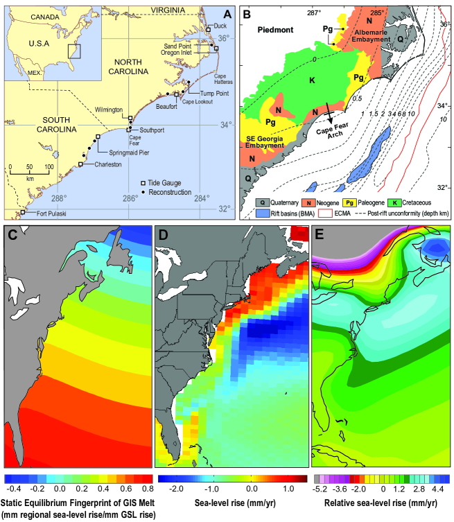
Figure 1: (A) Location map. (B) Map of regional shallow subsurface geology, post-rift unconformity, and large-scale structural geology (Dillon and P., 1988; Gohn, 1988; Grow and Sheridan, 1988; North Carolina Geological Survey, 2004). (C) Static-equilibrium fingerprint of RSL change from uniform melting of the Greenland Ice Sheet (Mitrovica et al, 2011), in units of mm RSL rise per mm GMSL rise. (D) Ocean dynamic contribution to RSL over 2006-2100 in the Community Earth System Model RCP 8.5 experiment from the Coupled Model Intercomparison Project Phase 5 (Taylor et al, 2012). (E) GIA contribution to RSL under the ICE-6G VM5b model (Engelhart et al, 2011)

2 Mechanisms for global, regional, and local relative sea-level changes

Relative sea level (RSL) is the difference in elevation between the solid Earth surface and the sea surface at a specific location and point in time. Commonly, it is time-averaged to minimize the influence of tides and is compared to the present as the reference period (Shennan et al, 2012). RSL averaged over all ocean basins yields an estimate of GMSL.

GMSL rise is driven primarily by (1) increases in ocean mass due to melting of land-based glaciers (e.g., Marzeion et al, 2012) and ice sheets (e.g., Shepherd et al, 2012) and (2) expansion of ocean water as it warms (e.g., Gregory, 2010). Changes in land water storage due to dam construction and groundwater withdrawal also contributed to 20th century GMSL change (e.g., Konikow, 2011). RSL differs from GMSL because of (1) factors causing vertical land motion, such as tectonics, sediment compaction, and groundwater withdrawal; (2) factors affecting both the height of the solid Earth and the height of Earth’s geoid, such as long-term GIA and the more immediate ‘sea-level fingerprint’ static-equilibrium response of the geoid and the solid Earth to redistribution of mass between land-based ice and the ocean; and (3) oceanographic and atmospheric factors affecting sea-surface height relative to the geoid, such as changes in ocean-atmospheric dynamics and the distribution of heat and salinity within the ocean (e.g., Kopp et al, 2014, 2015)

Along the U.S. Atlantic coast, the principal mechanism for regional departures from GMSL during the Holocene is GIA, which is the ongoing, multi-millennial response of Earth’s shape and geoid to large-scale changes in surface mass load (e.g., Clark et al, 1978) (Figure 1e). Growth and thickening of the Laurentide ice sheet during the last glaciation caused subsidence of land beneath the ice mass (Clark et al, 2009). A compensating outward flow in the mantle created a peripheral bulge around the ice margin in the U.S. mid-Atlantic region. In addition to uplifting the solid Earth in the U.S. mid-Atlantic region, these flows also increased the regional height of the geoid and reduced the global volume of the ocean basin. These latter two factors led to a rising sea-surface height in the U.S. mid-Atlantic region and thus a total RSL fall less than the regional uplift (Farrell and Clark, 1976). As the Laurentide ice sheet shrunk, mantle flow back toward the center of the diminishing ice sheet caused subsidence and progressive inward migration of the peripheral forebulge. One commonly used physical model of GIA (ICE-5G-VM2-90) yields contributions to 20th century sea-level rise of $\mathord{\sim}$1.3 mm/yr at New York City and $\mathord{\sim}$0.5 mm/yr at Wilmington, NC (Peltier, 2004), but exact values depend upon assumptions regarding ice-sheet history and mantle viscosity.

Along much of the U.S. Atlantic coast, the tectonic contribution to RSL change is assumed to be negligible over timescales of centuries to millennia (e.g., Rowley et al, 2013), but parts of the North Carolina coastal plain are underlain by the Cape Fear Arch (Sheridan, 1976) (Figure 1b). Geologic and geomorphic data suggest that uplift of the crest of the Cape Fear Arch began during the Pliocene (Wheeler, 2006) and is ongoing (Brown, 1978). Late Holocene rates of uplift (RSL fall) have been estimated at $\mathord{\sim}$0.2 $\pm$ 0.2 mm/yr (e.g., Marple and Talwani, 2004; van de Plassche et al, 2014).

The static-equilibrium ‘fingerprint’ contribution to RSL changes arises from the immediate response of Earth’s geoid, rotation, and elastic lithosphere to redistribution of mass between land ice and the ocean (Clark and Lingle, 1977; Mitrovica et al, 2011). As the mass of an ice sheet or glacier shrinks, sea-level rise is greater in areas geographically distal to the land ice than in areas close to it, primarily because the gravitational attraction between the ice mass and the ocean is reduced. Greenland Ice Sheet (GrIS) mass loss, for instance, generates a meridional sea-level gradient along the U.S. Atlantic coast (Figure 1c), where Maine experiences $\mathord{\sim}$30% of the global mean response, compared to $\mathord{\sim}60\%$ in North Carolina and $\mathord{\sim}80\%$ in south Florida. Melting of the West Antarctic Ice Sheet (WAIS), by contrast, causes a nearly uniform rise along the U.S. Atlantic coast (including North Carolina), which is about 20% higher than the global average due primarily to the effect of WAIS mass loss on Earth’s rotation (Mitrovica et al, 2009). Though the magnitude of sea-level fingerprints proximal to a changing ice mass is sensitive to the internal distribution of that mass, this sensitivity diminishes with distance. For example, at the distance of North Carolina, assumptions about the distribution of mass lost from GrIS have only an $\mathord{\sim}10\%$ effect on the fingerprint (i.e., a RSL effect equal to $\mathord{\sim}6\%$ of the global mean) (Mitrovica et al, 2011).

Oceanographic effects change sea-surface height relative to the geoid (e.g., Kopp et al, 2010). They include both global mean thermal expansion and regional changes in ocean-atmospheric dynamics and in the distribution of heat and salinity within the ocean. For example, changes in the Gulf Stream affect sea level in the western North Atlantic Ocean (e.g., Kienert and Rahmstorf, 2012; Ezer et al, 2013). As observed by satellite altimetry, the dynamic sea-surface height off of New Jersey averages $\mathord{\sim}$60 cm lower than the height off of Bermuda. By contrast, off the North Carolina coast, the dynamic sea-surface height averages $\mathord{\sim}30$ cm lower than off Bermuda, and this difference diminishes much more quickly off shore than it does north of Cape Hatteras, where the Gulf Stream separates from the U.S. Atlantic coast and turns toward northern Europe (Yin and Goddard, 2013). Ocean modeling shows that a slower Gulf Stream, which can be caused by a weaker Atlantic Meridional Overturning Circulation or by shifting winds, would reduce these sea-level gradients, increasing sea level along the U.S. Atlantic coast north of Cape Hatteras (Figure 1d). A northward shift in the position of the Gulf Stream, which could result from a migration of the Intertropical Convergence Zone (ITCZ), would similarly raise mid-Atlantic sea levels. In contrast, sea-surface height in coastal regions south of Cape Hatteras is less influenced by changes in the Gulf Stream (Yin and Goddard, 2013).

Locally in North Carolina, RSL also changes in response to sediment compaction (Brain et al, 2015), groundwater withdrawal (Lautier, 2006), and tidal-range shifts. North Carolina is partly located within the Albemarle Embayment (Figure 1b), a Cenozoic depositional basin (Foyle and Oertel, 1997) stretching from the Norfolk Arch at the North Carolina/Virginia border to southern Pamlico Sound at the Cape Lookout High. The embayment is composed of $\mathord{\sim}1.5$ km thick post-rift sedimentary rocks and Quaternary unconsolidated sediments (e.g., Gohn, 1988), currently undergoing compaction (e.g., van de Plassche et al, 2014).

The influence of local factors on regional RSL reconstructions is minimized by using proxy and instrumental data from multiple sites. For example, Kemp et al (2011) concluded that local factors were not the primary driving mechanisms for RSL change in North Carolina over the last millennium, because the trends reconstructed at two sites located $\mathord{>}100$ km apart in different water bodies closely agree.

3 Methods

3.1 Historical reconstruction

Tide gauges provide historic measurements of RSL for specific locations (Figure 1a). In North Carolina, there are two long-term tide-gauge records: Southport (covering 1933-1954, 1976-1988, and 2006-2007) and Wilmington (covering 1935 to present). Both have limitations: Southport has temporal gaps in the record, while the Wilmington record was influenced by deepening of the navigational channels, which increased the tidal range (Zervas, 2004). There are also shorter records from Duck (1978 to present), Oregon Inlet (1977 and 1994 to present), and Beaufort (1953-1961, 1966-1967, and 1973 to present), which we also include in our analysis.

Geological reconstructions provide proxy records of pre-20th century RSL. Our database of Holocene RSL reconstructions from North Carolina includes 107 discrete sea-level constraints from individual core samples collected at a suite of sites (Horton et al, 2009; Engelhart and Horton, 2012; van de Plassche et al, 2014). It also includes two continuous Common Era RSL reconstructions, from Tump Point (spanning the last $\mathord{\sim}$1000 years) and Sand Point (spanning the last $\mathord{\sim}$2000 years), produced using ordered samples from cores of salt-marsh sediment (Kemp et al, 2011) (Figure 1a). Salt marshes from the U.S. Atlantic Coast provide higher-resolution reconstructions than other sea-level proxies (in North Carolina, $<0.1$ m vertically and $\pm$ 1 to $\pm$ 71 y geochronologically). The combination of an extensive set of Holocene sea-level index points, multiple, high-resolution Common Era reconstructions, and tide-gauge measurements makes North Carolina well suited to evaluating past sea-level changes.

We fit the proxy and tide-gauge observations to a spatio-temporal Gaussian process (GP) statistical model of the Holocene RSL history of the U.S. Atlantic Coast. The model is similar to that of Kopp (2013), though with a longer temporal range and with geochronological uncertainty accommodated through the noisy-input GP method of McHutchon and Rasmussen (2011). To provide regional context, the fitted data also include records from outside of North Carolina, in particular salt-marsh reconstructions from New Jersey (Kemp et al, 2013) and Florida (Kemp et al, 2014) and all U.S. Atlantic Coast tide-gauge records in the Permanent Service for Mean Sea Level (2014) database with $\mathord{>}60$ years of data. To aid comparison with the proxy reconstructions, tide-gauge measurements were incorporated into the analysis as decadal averages. The GP model represents sea level as the sum of spatially-correlated low-frequency (millennial), medium-frequency (centennial) and high-frequency (decadal) processes. Details are provided in the Supporting Information. All estimated rates of past RSL change in this paper are based on application of the GP model to the combined data set and are quoted with $2\sigma$ uncertainties.

3.2 Future projections

Several data sources are available to inform sea-level projections, including process models of ocean and land ice behavior (e.g., Taylor et al, 2012; Marzeion et al, 2012), statistical models of local sea-level processes (Kopp et al, 2014), expert elicitation on ice-sheet responses (Bamber and Aspinall, 2013) and expert assessment of the overall sea-level response (Church et al, 2013; Horton et al, 2014). Kopp et al (2014) synthesized these different sources to generate self-consistent, probabilistic projections of local sea-level changes around the world under different future emission trajectories.

Combined with historical records of storm tides, RSL projections provide insight into the changes in expected flood frequencies over the 21st century. We summarize the RSL projections of Kopp et al (2014) for North Carolina and apply the method of Tebaldi et al (2012) and Kopp et al (2014) to calculate their implications for flood-return periods.

Note that the projections of Kopp et al (2014) are not identical to those of the expert assessment of the Intergovernmental Panel on Climate Change (IPCC)’s Fifth Assessment Report (Church et al, 2013). The most significant difference arises from the use of a self-consistent framework for estimating a complete probability distribution of RSL change, not just the likely (67% probability) GMSL projections of the IPCC. Kopp et al (2014) and the IPCC estimate similar but not identical likely 21st century GMSL rise (under RCP 8.5, 62–100 cm vs. 53–97 cm, respectively; under RCP 2.6, 37–65 cm vs. 28–60 cm).

4 Holocene sea-level change in North Carolina

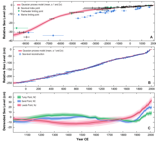
Figure 2: (a) Holocene RSL in North Carolina, showing a representative GP estimate for central North Carolina (red), as well all index points (crosses), marine limiting points (blue upward triangles), and freshwater limiting points (green downward triangles) from North Carolina. Index/limiting points shown with 2$\sigma$ error bars. (b) RSL over the Common Era at Sand Point, North Carolina. (c) RSL detrended with respect to the 1000-1800 CE average rate for North Carolina (NC) and New Jersey (NJ). GP estimates are shown with 1$\sigma$ (dark shading) and 2$\sigma$ (light shading) errors.

RSL rose rapidly during the early and mid-Holocene, increasing in central North Carolina from -30.1 $\pm$ 1.8 m at 9000 BCE to -4.1 $\pm$ 0.7 m at 2000 BCE (Fig. 2a). The rate of RSL rise decreased over time, as a result of declining input from shrinking land ice reservoirs and slowing GIA (Peltier, 2004; Milne and Mitrovica, 2008), from a millennially-averaged rate of 6.8 $\pm$ 1.2 mm/yr at 8000 BCE to 0.8 $\pm$ 1.0 mm/yr at 2500 BCE. A declining GIA rate with increasing distance from the center of the Laurentide ice sheet (Engelhart et al, 2009), along with a contribution from tectonic uplift along the Cape Fear Arch (van de Plassche et al, 2014), caused spatial variability in the rate of Common Era RSL rise along the U.S. Atlantic coast and within North Carolina (Fig. 3a). At Sand Point in northern North Carolina, RSL rose from -2.38 $\pm$ 0.06 m at 0 CE to -0.37 $\pm$ 0.05 m by 1800 CE, an average rate of 1.11 $\pm$ 0.03 mm/yr. In the Wilmington area, the estimated average rate of RSL rise from 0 to 1800 CE was 0.8 $\pm$ 0.2 mm/yr (Fig. 3a-b; Table S-1).

Century-average rates of RSL change varied around these long-term means. For example, between 1000 and 1800 CE at Sand Point, century-average rates of RSL change ranged from a high of 1.7 $\pm$ 0.5 mm/yr (in the 12th century) to a low of 0.9 $\pm$ 0.5 mm/yr (in the 16th century) (Figure 2b). Synchronous sea-level changes occurred in southern NC over the same period of time (Kemp et al, 2011). However, the sign of the North Carolina RSL rate changes contrasts with that reconstructed at sites further north in New Jersey (Kopp, 2013) (Figure 2c). This contrast suggests a role for changes in ocean and atmosphere circulation, such as a shift in the position or strength of the Gulf Stream, in explaining these variations. A strengthening of the Gulf Stream (the opposite of the pattern depicted in Figure 1d) would be consistent with the observations. The absence of similarly timed variations in Florida (Kemp et al, 2014) excludes a significant contribution from the static-equilibrium fingerprint of GrIS mass changes (Figure 1c).

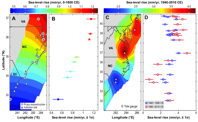
Figure 3: (a) Pre-Industrial Common Era rate of RSL rise (0-1800 CE; mm/yr). Diamonds: proxy sites; grey circles: selected tide gauges and continuous proxy records (as in Tables S-1 and S-2). Uncolored areas have $1\sigma$ uncertainty $\mathord{>}0.15$ mm/yr. (b) shows estimates at indicated tide-gauge and continuous proxy record sites (1$\sigma$ errors). (c) 1940-2010 rate of RSL rise. Diamonds: tide-gauge locations with $\mathord{>}60$ years of data. Uncolored areas have $1\sigma$ uncertainty $\mathord{>}0.5$ mm/yr. (d) 1940-1980 (blue squares) and 1980-2010 (red circles) rates of RSL rise at tide-gauge sites.

5 Twentieth-century sea-level changes in North Carolina

The most prominent feature in the North Carolina Common Era sea-level record is the acceleration of the rate of rise between the 19th and 20th centuries (Figure 2b-c). At Sand Point, the average rate of RSL rise over the 19th century (1.0 $\pm$ 0.5 mm/yr) was within the range of previous Common Era variability and close to the long-term average. By contrast, it is extremely likely ($P=0.95$) that the 2.7 $\pm$ 0.5 mm/yr experienced in the 20th century was not exceeded in any century since at least the 10th century BCE (which had a rate of 1.2 $\pm$ 1.6 mm/yr). Average 20th century RSL rates range from 2.1 $\pm$ 0.5 mm/yr at Wilmington to 3.5 $\pm$ 0.3 mm/yr at Tump Point (Table S-1).

Spatial patterns of sea-level variability are detectable at higher temporal frequencies in the tide-gauge record (Kopp, 2013; Yin and Goddard, 2013) (Figure 3c-d; Table S-2). From 1940 to 1980 CE, sea-level rise in both North Carolina and the U.S. mid-Atlantic region exceeded the global mean. At Wilmington and Duck, the average rates were 2.3 $\pm$ 0.7 mm/yr and $3.3\pm 0.9$ mm/yr, respectively, compared to 2.8 $\pm$ 0.6 mm/yr at New York City and a GMSL rise of $0.8\pm 0.8$ mm/yr (Hay et al, 2015). This pattern changed over the interval from 1980 to 2010 CE, when the rate of GMSL rise increased to $2.5\pm 0.5$ mm/yr while rates of RSL rise south of Cape Hatteras remained stationary or decreased (1.7 $\pm$ 1.0 mm/yr at Beaufort, 0.7 $\pm$ 0.9 mm/yr at Wilmington, and 1.2 $\pm$ 1.1 mm/yr at Southport). In contrast, sites north of Cape Hatteras experienced a significant increase in rate; at New York City, for example, RSL rose at 3.7 $\pm$ 0.9 mm/yr.

Several recent papers identified this regional phenomenon in the northeastern U.S. as a “hot spot” of sea-level acceleration (Sallenger et al, 2012; Boon, 2012; Ezer and Corlett, 2012; Kopp, 2013). Less attention has been paid to its counterpart in the southeastern U.S., which might be regarded as a “hot spot” of deceleration, especially when considered in the context of the GMSL acceleration occurring over the same interval. The pattern of a sea-level increase north of Cape Hatteras and sea-level decrease south of Cape Hatteras is consistent with a northward migration of the Gulf Stream (Yin and Goddard, 2013; Rahmstorf et al, 2015). It is also consistent with the dominant spatial pattern of change seen in the North Carolina and New Jersey proxy reconstructions from the 16th through the 19th century (Figure 2c). Dredging has, however, contaminated some North Carolina tide gauges, rendering a simple assessment of the ocean dynamic contribution during the 20th century challenging.

6 Future sea-level projections for North Carolina

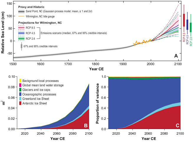
Figure 4: (a) GP estimate of sea-level at Sand Point (black), annual Wilmington tide-gauge data (orange), and Kopp et al (2014) projections for RCP 8.5 (red), 4.5 (blue), and 2.6 (green). Shading/dashed lines = 67%/95% credible intervals. Bars and whiskers represent 67% and 95% credible intervals of 2100 CE projections. All heights relative to 2000 CE. (b-c) Sources of uncertainty in RCP 8.5 20-year-average sea-level rise projection at Wilmington, shown in units of (b) variance and (c) fractional variance as in Kopp et al (2014).

Table 1: Projected sea-level rise in North Carolina under RCP 8.5 and RCP 2.6

cm	RCP 8.5					RCP 2.6
	50	17–83	5–95	0.5–99.5	99.9	50	17–83	5–95	0.5–99.5
DUCK, NC
2030	23	16–29	12–33	6–39	43	22	17–28	12–32	7–38
2050	41	31–51	24–59	15–72	83	37	28–46	22–53	13–66
2100	100	73–129	54–154	29–214	304	70	50–93	36–113	17–181
2150	160	124–206	103–255	76–425	627	99	71–136	56–184	39–357
2200	225	166–304	134–394	99–715	1055	131	80–196	58–287	33–607
WILMINGTON, NC
2030	17	12–23	8–27	3–33	36	17	12–21	9–25	4–30
2050	33	24–42	18–48	10–61	75	29	21–36	16–42	9–55
2100	82	58–109	42–132	20–194	281	54	36–74	24–94	8–162
2150	135	101–180	81–230	57–395	596	77	48–113	34–161	16–334
2200	194	136–273	105–364	74–678	1016	101	50–166	27–257	3–575
Values represent two-decade averages and are in cm above 1990–2010 (‘2000’) mean sea level.
Columns correspond to different projection probabilities. For example, the “5-95” columns
correspond to the 5th to 95th percentile; in IPCC terms, the ‘very likely’ range.
The RCP 8.5 99.9th percentile corresponds to the maximum level physically possible.

The integrated assessment and climate modeling communities developed Representative Concentration Pathways (RCPs) to describe future emissions of greenhouse gases consistent with varied socio-economic and policy scenarios (Van Vuuren et al, 2011). These pathways provide boundary conditions for projecting future climate and sea-level changes. RCP 8.5 is consistent with high-end business-as-usual emissions. RCP 4.5 is consistent with moderate reductions in greenhouse gas emissions, while RCP 2.6 requires strong emissions reductions. These three RCPs respectively yield likely ($P=0.67$) global mean temperature increases in 2081-2100 CE of 3.2–5.4^∘C, 1.7–3.2^∘C, and 0.9–2.3^∘C above 1850-1900 CE levels (Collins et al, 2013).

A bottom-up assessment of the factors contributing to sea-level change (Kopp et al, 2014) indicates that, regardless of the pathway of future emissions, it is virtually certain ($P>0.998$) that both Wilmington and Duck will experience a RSL rise over the 21st century and very likely ($P>0.90$) that the rate of that rise will exceed the rate observed during the 20th century. Below, we summarize the bottom-up projections of Kopp et al (2014) for Wilmington and Duck, NC, which bracket the latitudinal extent and degree of spatial variability across the state (Tables 1, S-3, S-4, S-5).

Under the high-emissions RCP 8.5 pathway, RSL at Wilmington will very likely ($P=0.90$) rise by 8–27 cm (median of 17 cm) between 2000 and 2030 CE and by 18–48 cm (median of 33 cm) between 2000 and 2050 CE (Figure 4a). Projected RSL rise varies modestly across the state, with a very likely rise of 12–33 cm (median 23 cm) between 2000 and 2030 CE and of 24–59 cm (median of 41 cm) between 2000 and 2050 CE at Duck. Because sea level responds slowly to climate forcing, projected RSL rise before 2050 CE can be reduced only weakly ($\mathord{\sim}$3-6 cm) through greenhouse gas mitigation.

It is important to consider these numbers in the context of the background variability in annual-mean and decadal-mean RSL. Relative to 20-year-mean RSL, annual-mean RSL as measured by the Wilmington tide gauge has a standard deviation of $\mathord{\sim}8$ cm, so the median projection for 2030 CE is only slightly above twice the standard deviation. It would therefore not be surprising to see an isolated year with RSL as high as that projected for 2030 CE even in the absence of a long-term trend. However, consecutive years of that height would be unexpected, as decadal-mean RSL has a standard deviation of $\mathord{\sim}1$ cm. Given the magnitude of decadal variability, however, differences in projections of $\mathord{<}\mathord{\sim}4$ cm should not be viewed as significant.

Reductions in greenhouse gases over the course of the 21st century can significantly affect sea-level rise after 2050 CE. Under the high-emissions RCP 8.5 pathway, RSL at Wilmington is very likely to rise by 42–132 cm (median of 82 cm) between 2000 and 2100 CE, while under the low-emissions RCP 2.6 pathway, it is very likely to rise by 24–94 cm (median of 54 cm). The maximum physically possible 21st century sea-level rise is significantly higher ($\mathord{\sim}$280 cm), although the estimated probability of such an outcome is extremely low ($P\approx 0.001$) (Kopp et al, 2014). Projected RSL rise varies modestly across the state, with a very likely rise of 54–154 cm (median of 100 cm) under RCP 8.5 and 36–113 cm (median of 70 cm) under RCP 2.6 at Duck, a difference from Wilmington of $\mathord{\sim}$12–22 cm.

Uncertainty in projected RSL rise in North Carolina stems from two main sources: the (1) oceanographic and (2) Antarctic ice sheet responses to climate change. The former source dominates the uncertainty through most of the century, with the Antarctic response coming to play a roughly equal role by the end of the century (Figure 4b-c). At Wilmington, under RCP 8.5, ocean dynamics is likely ($P=0.67$) to contribute -9 to +17 cm (median 5 cm) to 21st century sea-level rise. The dynamic contribution increases to the north, with -9 to +25 cm (median 8 cm) likely at Duck. These contributions are less than those in the northeastern United States; for example, at New York, ocean dynamics are likely to contribute -6 to +35 cm (median 14 cm).

The GrIS contribution to uncertainty in North Carolina RSL change is smaller than the Antarctic contribution because of two factors. First, GrIS makes a smaller overall contribution to GMSL uncertainty, because GrIS mass change is dominated by surface mass balance, while the behavior of WAIS is dominated by more complex and uncertain ocean/ice sheet dynamics. Second, the GrIS contribution to North Carolina RSL change and to its uncertainty is diminished by the static-equilibrium fingerprint effect to about 60% of its global mean value.

7 Implications of sea-level rise for flood risk and economic damages

Based on historical storm tides, the ‘1-in-10 year’ flood (i.e., the flood level with a probability of 10% in any given year) at the Wilmington tide gauge is 0.60 m above current mean higher high water (MHHW). In the absence of sea-level rise, one would expect three such floods over a 30-year period. Assuming no increase in the height of storm-driven flooding relative to mean sea level and accounting for the probability distribution of projected sea-level rise as in Kopp et al (2014), seven similar magnitude floods are expected between 2000 and 2030 (regardless of RCP). Between 2000 and 2050, the expected number of years experiencing a flood at 0.60 m above current MHHW increases from 5 to 21. After 2050, regardless of RCP, almost every year is expected to see at least one flood at 0.60 m above current MHHW. Similarly, the expected number of 0.93 m ‘1-in-100 year’ floods will increase with projected sea-level rise. The ‘1-in-100 year’ flood is expected about 1.6–1.8 times between 2000 and 2050 (rather than the 0.5 times expected in the absence of sea-level rise). During the second half of the century, ‘1-in-100 year’ flooding is expected in 29 of 50 years under RCP 8.5 and 17 of 50 years under RCP 2.6.

Houser et al (2015) characterized the costs of projected sea-level rise and changes in flood frequency using the Risk Management Solutions North Atlantic Hurricane Model, which models wind and coastal flood damage to property and interrupted businesses caused by a database of tens of thousands of synthetic storm events. Under all RCPs, projected RSL rise in North Carolina would likely ($P=0.67$) place $\mathord{>}\$4$ billion of current property below MHHW by 2050 and $\mathord{>}\$17$ billion by 2100. Statewide (assuming fixed distribution and value of property), average annual insurable losses from coastal storms will very likely ($P=0.90$) increase by 4-17% between 2011 and 2030 and by 16-75% between 2011 and 2050 (regardless of RCP). By 2100, they are very likely to increase by 50-160% under RCP 8.5 and 20-150% under RCP 2.6 (Houser et al, 2015). Projected increases in the intensity of tropical cyclones under RCP 8.5 (Emanuel, 2013) may amplify the increase in losses by $\mathord{\sim}$1.5x by 2050 and $\mathord{\sim}$2.1x by 2100. These cost estimates assume a fixed distribution and valuation of property; intensification of development along the coastline will increase exposure and therefore cost, while protective measures will decrease exposure and cost.

8 Concluding remarks

North Carolina Session Law 2012-202/House Bill 819 requires assessment of future sea-level change trajectories that include “sea-level fall, no movement in sea level, deceleration of sea-level rise, and acceleration of sea-level rise.” Geological and historical records indicate that, over the last 11,000 years, North Carolina experienced periods of RSL deceleration and acceleration, but no periods of RSL stasis or fall.

• Millennially-averaged RSL rise in central North Carolina decelerated from 8000 BCE (6.8 $\pm$ 1.2 mm/yr) until 2500 BCE (0.8 $\pm$ 1.0 mm/yr).  
  

• From 0 to 1800 CE, average RSL rise rates within North Carolina varied from 1.11 $\pm$ 0.03 mm/yr in northern North Carolina to 0.8 $\pm$ 0.2 mm/yr in southern North Carolina (in the vicinity of the Cape Fear Arch, and farther away from the peripheral bulge). Century-average rates of sea-level change varied around these long-term means. Comparison of records along the U.S. Atlantic coast indicate that pre-Industrial Common Era sea-level accelerations and decelerations had a spatial pattern consistent with variability in the strength and/or position of the Gulf Stream.  
  

• It is extremely likely ($P=0.95$) that the accelerated rate of 20th century RSL rise at Sand Point, NC, (2.7 $\pm$ 0.5 mm/yr) had not been reached in any century since at least the 10th century BCE.  
  

• Between 1940-1980 and 1980-2010, sea level in North Carolina decelerated relative to the global mean and possibly in absolute terms (at Wilmington, from 2.3 $\pm$ 0.5 mm/yr to 0.7 $\pm$ 0.9 mm/yr; at Southport, from 2.5 $\pm$ 0.7 mm/yr to 1.2 $\pm$ 1.1 mm/yr), while sea-level rise accelerated north of Cape Hatteras. The spatial pattern and the magnitude of change are consistent with Gulf Stream variability.  
  

• It is virtually certain ($P=0.99$) that RSL rise at Wilmington between 2000 and 2050 will exceed 2.2 mm/yr, nearly three times the 0-1800 CE average rate. It is extremely likely ($P=0.95$) that it will exceed 3.2 mm/yr, in excess of the 20th century average of 2.2 $\pm$ 0.6 mm/yr. Under the high-emissions RCP 8.5 pathway, RSL is very likely to rise by 42–132 cm, and under the low-emissions RCP 2.6 pathway RSL is very likely to rise by 24–94 cm between 2000 and 2100. 
  

• Storm flooding in North Carolina will be increasingly exacerbated by sea-level rise. After 2050, the current ‘1-in-10 year’ flood is expected to occur in Wilmington almost every year and the ‘1-in-100 year’ flood is expected to occur in about 17–29 years. Assuming the current distribution of property and economic activity, average annual insurable losses statewide would very likely increase by 50-160% under RCP 8.5 and 20-150% under RCP 2.6.

Supporting Information: Spatio-temporal statistical model

The spatio-temporal sea-level field $f(\mathbf{x},t)$ is modeled as a sum of Gaussian processes (Rasmussen and Williams, 2006) with different characteristic spatial and temporal scales.

$$f(\mathbf{x},t) =l(\mathbf{x},t)+m(\mathbf{x},t)+h(\mathbf{x},t)$$ (S-1)

Each field has a prior mean of zero and spatially and temporally separable prior covariances given by

$$k_{l}(\mathbf{x}_{1},t_{1},\mathbf{x}_{2},t_{2}) =\sigma_{l}^{2}\cdot C_{\frac{3}{2}}(|t_{2}-t_{1}|,\tau_{l})\cdot C_{\frac{5}{2}}(r(\mathbf{x}_{1},\mathbf{x}_{2}),\gamma_{l})$$ (S-2)

$$k_{m}(\mathbf{x}_{1},t_{1},\mathbf{x}_{2},t_{2}) =\sigma_{m}^{2}\cdot C_{\frac{3}{2}}(|t_{2}-t_{1}|,\tau_{m})\cdot C_{\frac{1}{2}}(r(\mathbf{x}_{1},\mathbf{x}_{2}),\gamma_{m})$$ (S-3)

$$k_{h}(\mathbf{x}_{1},t_{1},\mathbf{x}_{2},t_{2}) =\sigma_{h}^{2}\cdot C_{\frac{3}{2}}(|t_{2}-t_{1}|,\tau_{h})\cdot C_{\frac{1}{2}}(r(\mathbf{x}_{1},\mathbf{x}_{2}),\gamma_{m})$$ (S-4)

where $C_{\nu}(r,\lambda)$ is a Matérn covariance function with scale $\lambda$ and smoothness parameter $\nu$. Here $\sigma_{i}^{2}$ are the amplitudes of the prior variances, $\tau_{i}$ are characteristic time scales, $\gamma_{i}$ are characteristic length scales, and $r(\mathbf{x}_{1},\mathbf{x}_{2})$ is the angular distance between $\mathbf{x}_{1}$ and $\mathbf{x}_{2}$.

The observations $y(\mathbf{x},t^{\prime})$ are modeled as

$$y(\mathbf{x},t^{\prime}) =f(\mathbf{x},t+\epsilon_{t})+w(\mathbf{x},t^{\prime})+\epsilon_{y}+y_{0}(\mathbf{x}),$$ (S-6)

where $t^{\prime}$ is the true age of the observation, $t$ the mean observed age, $w$ a process that captures sea-level variability at a sub-decadal level (which we treat here as noise), $\epsilon_{t}$ and $\epsilon_{y}$ are errors in the age and sea-level observations, and $y_{0}$ is a site-specific datum offset. For tide gauges, $\epsilon_{t}$ is zero and $\epsilon_{y}$ is estimated during a smoothing process (see below) in which annual data are assumed to have uncorrelated, normally distributed noise with standard deviation 3 mm. For proxy data, $\epsilon_{t}$ and $\epsilon_{y}$ are treated as independent and normally distributed, with a standard deviation specified for each observation based on the original publication. The sub-decadal and datum offset processes are modeled as Gaussian processes with mean zero and prior covariances given by

$$k_{w}(\mathbf{x}_{1},t_{1},\mathbf{x}_{2},t_{2}) =\sigma_{w}^{2}\delta(t_{1},t_{2})\delta(\mathbf{x}_{1},\mathbf{x}_{2})$$ (S-7)

$$k_{0}(\mathbf{x}_{1},\mathbf{x}_{2}) =\sigma_{0}^{2}\delta(\mathbf{x}_{1},\mathbf{x}_{2}),$$ (S-8)

where $\delta(\mathbf{x}_{1},\mathbf{x}_{2})$ is the Kronecker delta function. Geochronological uncertainties are incorporated using the noisy-input Gaussian process method of McHutchon and Rasmussen (2011):

$$y(\mathbf{x},t^{\prime}) \approx f(\mathbf{x},t^{\prime})+\epsilon_{t}f^{\prime}(\mathbf{x},t^{\prime})+w(\mathbf{x},t)+\epsilon_{y}+y_{0}(\mathbf{x}).$$ (S-9)

The low-frequency process $l(\mathbf{x},t)$ (physically corresponding to GIA, tectonics, long-term sediment compaction, and long-term GMSL change), medium-frequency process $m(\mathbf{x},t)$, and high-frequency process $h(\mathbf{x},t)$ all have Matérn temporal covariance functions with smoothness parameter $\nu=1.5$, implying a functional form in which the first derivative is everywhere defined. The low-frequency process is assumed to vary smoothly over space ($\nu=2.5$), while the medium- and high-frequency process are allowed to vary more roughly ($\nu=0.5$). The length scale $\gamma_{m}$ is required to be equal for the medium- and high-frequency processes, as both are expected to reflect similar oceanographic processes operating on different timescales.

The hyperparameters $\mathbf{\Theta}=\{\sigma_{l},\sigma_{m},\sigma_{h},\sigma_{w},\sigma_{0},\tau_{l},\tau_{m},\tau_{w},\gamma_{l},\gamma_{m}\}$ are set through a three-step optimization process. First, the hyperparameters of a simplified model, in which a linear term replaces the low-frequency process, are globally optimized through simulated annealing to maximize the marginal likelihood $\mathcal{L}(\mathbf{\Theta}|\mathbf{y}_{1})$, where $\mathbf{y}_{1}$ is the set of post-1000 BCE observations. Second, the hyperparameters of $m(\mathbf{x},t)$, $h(\mathbf{x},t)$ and $w(\mathbf{x},t)$ are fixed. The remaining hyperparameters of the full model – the amplitude, scales, and spatial roughness of the low-frequency process, as well as the datum offset – are globally optimized so as to maximize the marginal likelihood $\mathcal{L}(\mathbf{\Theta}|\mathbf{y}_{2})$, where $\mathbf{y}_{2}$ is the complete data set . Finally, all the hyperparameters are locally optimized to maximize the marginal likelihood $\mathcal{L}(\mathbf{\Theta}|\mathbf{y}_{2})$. This multi-step process improves performance relative to globally optimizing all hyperparameters simultaneously and is guided by the recognition that the long-term, low-resolution data provide the greatest insight into the lowest-frequency processes while the salt-marsh and tide-gauge data provide the greatest insight into the medium-frequency and high-frequency processes. The optimized time scales of the high-, medium- and low-frequency processes are respectively $\tau_{l}=14.5$ kyr, $\tau_{m}=296$ years and $\tau_{h}=6.3$ years; other hyperparameters are shown in Table S-6.

Annual mean tide-gauge data are decadally averaged prior to incorporation into the analysis. To accommodate data gaps estimate the covariance of the decadal averages, we fit each annual record $y_{j}(t)$ separately with the model

$$y_{j}(t)=\alpha_{j}(t-t_{0})+d_{j}(t)+y_{0,j},$$ (S-10)

where $\alpha_{j}$ is a slope, $t_{0}$ a reference time period, and $d_{j}(t)$ a Gaussian process with prior mean zero and a prior Matérn covariance. Hyperparameters are optimized on a site-by-site basis to maximize their marginal likelihood. Decadal averages, including their covariances, are then taken from the interpolated process $y_{j}(t)$.

Table S-1: Common Era sea-level rates (mm/yr)

Site	Lat	Long	0-1800	1000-1500	1500-1800	1800-1900	1900-2000
GMSL							$1.3\pm 0.2$
New York, NY	40.7	-74.0	1.69 $\pm$ 0.18	1.5 $\pm$ 0.5	1.9 $\pm$ 0.7	2.1 $\pm$ 0.7	2.9 $\pm$ 0.3
Leeds Point, NJ	39.5	-74.4	1.52 $\pm$ 0.09	1.2 $\pm$ 0.2	1.7 $\pm$ 0.4	2.4 $\pm$ 0.8	3.8 $\pm$ 0.5
Cape May, NJ	39.1	-74.8	1.46 $\pm$ 0.10	1.2 $\pm$ 0.2	1.5 $\pm$ 0.3	2.2 $\pm$ 0.6	3.7 $\pm$ 0.5
Sewell’s Point, VA	37.0	-76.3	1.15 $\pm$ 0.18	1.2 $\pm$ 0.5	0.9 $\pm$ 0.6	1.6 $\pm$ 0.9	4.2 $\pm$ 0.5
Duck, NC	36.2	-75.8	1.13 $\pm$ 0.08	1.4 $\pm$ 0.3	1.0 $\pm$ 0.4	1.2 $\pm$ 0.6	3.1 $\pm$ 0.6
Sand Point, NC	35.9	-75.7	1.11 $\pm$ 0.03	1.4 $\pm$ 0.1	1.0 $\pm$ 0.2	1.0 $\pm$ 0.5	2.7 $\pm$ 0.5
Oregon Inlet, NC	35.8	-75.6	1.11 $\pm$ 0.07	1.4 $\pm$ 0.2	1.0 $\pm$ 0.3	1.1 $\pm$ 0.6	2.6 $\pm$ 0.5
Tump Point, NC	35.0	-76.4	0.87 $\pm$ 0.11	1.2 $\pm$ 0.2	0.7 $\pm$ 0.2	1.4 $\pm$ 0.4	3.5 $\pm$ 0.3
Beaufort, NC	34.7	-76.7	0.83 $\pm$ 0.13	1.2 $\pm$ 0.3	0.7 $\pm$ 0.4	1.2 $\pm$ 0.7	2.9 $\pm$ 0.5
Wilmington, NC	34.2	-78.0	0.76 $\pm$ 0.18	1.0 $\pm$ 0.5	0.7 $\pm$ 0.6	0.9 $\pm$ 1.0	2.1 $\pm$ 0.5
Southport, NC	33.9	-78.0	0.70 $\pm$ 0.18	0.9 $\pm$ 0.5	0.6 $\pm$ 0.6	0.9 $\pm$ 1.0	2.3 $\pm$ 0.6
Charleston, SC	32.8	-79.9	0.53 $\pm$ 0.21	0.6 $\pm$ 0.6	0.4 $\pm$ 0.7	1.1 $\pm$ 1.1	2.9 $\pm$ 0.5
Fort Pulaski, GA	32.0	-80.9	0.47 $\pm$ 0.19	0.5 $\pm$ 0.5	0.3 $\pm$ 0.7	1.0 $\pm$ 1.1	2.7 $\pm$ 0.5
Nassau, FL	30.6	-81.7	0.41 $\pm$ 0.05	0.5 $\pm$ 0.2	0.4 $\pm$ 0.3	0.7 $\pm$ 0.8	1.9 $\pm$ 0.4
Errors are $\pm 2\sigma$. GMSL from Hay et al (2015).

Table S-2: Industrial era sea-level rates (mm/yr)

Site	Lat	Long	1860-1900	1900-1940	1940-1980	1980-2010
GMSL				$1.2\pm 1.1$	$0.8\pm 0.8$	$2.5\pm 0.5$
New York, NY	40.7	-74.0	2.5 $\pm$ 0.7	2.7 $\pm$ 0.7	2.8 $\pm$ 0.6	3.7 $\pm$ 0.9
Atlantic City, NJ	39.4	-74.4	3.0 $\pm$ 1.1	3.7 $\pm$ 0.9	3.7 $\pm$ 0.7	4.6 $\pm$ 1.0
Cape May, NJ	39.1	-74.8	2.8 $\pm$ 1.0	3.4 $\pm$ 0.9	3.4 $\pm$ 0.8	4.4 $\pm$ 1.1
Sewell’s Point, VA	37.0	-76.3	2.3 $\pm$ 1.3	3.9 $\pm$ 1.1	4.0 $\pm$ 0.6	5.0 $\pm$ 0.9
Duck, NC	36.2	-75.8	1.7 $\pm$ 1.1	3.2 $\pm$ 1.0	3.3 $\pm$ 0.9	2.9 $\pm$ 1.0
Sand Point, NC	35.9	-75.7	1.4 $\pm$ 1.0	3.0 $\pm$ 0.9	3.0 $\pm$ 0.8	2.0 $\pm$ 1.1
Oregon Inlet, NC	35.8	-75.6	1.5 $\pm$ 1.0	3.0 $\pm$ 0.9	3.0 $\pm$ 0.9	1.7 $\pm$ 1.1
Tump Point, NC	35.0	-76.4	2.0 $\pm$ 0.9	4.0 $\pm$ 0.8	3.7 $\pm$ 0.7	2.0 $\pm$ 1.1
Beaufort, NC	34.7	-76.7	1.7 $\pm$ 1.1	3.5 $\pm$ 1.0	3.1 $\pm$ 0.8	1.7 $\pm$ 1.0
Wilmington, NC	34.2	-78.0	1.3 $\pm$ 1.3	2.5 $\pm$ 1.2	2.3 $\pm$ 0.7	0.7 $\pm$ 0.9
Southport, NC	33.9	-78.0	1.4 $\pm$ 1.4	2.5 $\pm$ 1.2	2.5 $\pm$ 0.7	1.2 $\pm$ 1.1
Charleston, SC	32.8	-79.9	1.7 $\pm$ 1.5	2.8 $\pm$ 1.1	3.0 $\pm$ 0.7	2.9 $\pm$ 0.9
Fort Pulaski, GA	32.0	-80.9	1.5 $\pm$ 1.4	2.4 $\pm$ 1.2	2.8 $\pm$ 0.7	3.0 $\pm$ 0.9
Fernandina Beach, FL	30.7	-81.5	1.2 $\pm$ 1.3	1.5 $\pm$ 0.7	1.9 $\pm$ 0.7	2.3 $\pm$ 0.9
Errors are $\pm 2\sigma$. GMSL from Hay et al (2015).

Table S-3: Projected sea-level rise in North Carolina by decade under RCPs 8.5 and 2.6

cm	RCP 8.5					RCP 2.6
	50	17–83	5–95	0.5–99.5	99.9	50	17–83	5–95	0.5–99.5
DUCK, NC
2010	7	5–9	4–10	1–12	13	7	5–9	3–11	1–13
2020	14	11–18	8–21	4–25	27	15	11–18	9–21	5–24
2030	23	16–29	12–33	6–39	43	22	17–28	12–32	7–38
2040	31	24–39	18–45	11–53	60	30	22–37	17–43	10–51
2050	41	31–51	24–59	15–72	83	37	28–46	22–53	13–66
2060	52	40–65	32–74	20–93	120	44	33–57	25–66	13–85
2070	64	49–80	39–92	24–118	158	51	38–65	28–77	15–103
2080	76	57–95	45–111	27–146	201	57	43–74	32–87	17–125
2090	88	66–112	51–132	30–179	250	63	46–83	34–100	18–151
2100	100	73–129	54–154	29–214	304	70	50–93	36–113	17–181
2150	160	124–206	103–255	76–425	627	99	71–136	56–184	39–357
2200	225	166–304	134–394	99–715	1055	131	80–196	58–287	33–607
WILMINGTON, NC
2010	5	3–7	2–8	0–10	11	5	4–7	2–8	1–10
2020	11	8–15	5–17	1–21	22	11	8–14	6–16	4–18
2030	17	12–23	8–27	3–33	36	17	12–21	9–25	4–30
2040	25	18–31	13–36	6–44	51	23	17–29	12–34	6–42
2050	33	24–42	18–48	10–61	75	29	21–36	16–42	9–55
2060	42	31–53	24–62	13–80	107	34	25–44	18–52	9–70
2070	52	39–66	29–78	17–103	142	39	28–51	20–61	9–88
2080	62	46–79	35–94	19–130	183	44	31–58	23–71	10–111
2090	73	53–94	40–113	21–162	229	49	34–66	24–82	10–135
2100	82	58–109	42–132	20–194	281	54	36–74	24–94	8–162
2150	135	101–180	81–230	57–395	596	77	48–113	34–161	16–334
2200	194	136–273	105–364	74–678	1016	101	50–166	27–257	3–575
Values represent two-decade averages and are in cm above 1990–2010 (‘2000’) mean sea level.
Columns correspond to different projection probabilities. For example, the “5-95” columns
correspond to the 5th to 95th percentile; in IPCC terms, the ‘very likely’ range.
The RCP 8.5 99.9th percentile corresponds to the maximum level physically possible.

Table S-4: Projected sea-level rise in North Carolina by decade under RCP 4.5

cm	RCP 4.5
	50	17–83	5–95	0.5–99.5
DUCK, NC
2010	7	5–9	3–11	1–13
2020	14	11–18	8–21	4–25
2030	22	17–27	13–31	8–36
2040	30	24–37	19–42	13–50
2050	39	30–47	23–54	15–67
2060	47	36–59	28–68	17–86
2070	56	42–71	32–82	18–108
2080	64	48–82	37–96	21–130
2090	72	54–93	41–110	23–158
2100	81	60–105	45–126	25–188
2150	121	84–164	60–209	30–374
2200	160	101–232	67–315	24–618
WILMINGTON, NC
2010	5	3–7	1–9	-1–11
2020	11	7–14	5–17	1–20
2030	17	12–21	9–24	5–29
2040	23	17–29	13–33	8–40
2050	30	22–37	17–43	10–55
2060	37	27–47	20–55	11–72
2070	44	32–56	24–66	12–91
2080	51	37–66	27–78	14–114
2090	57	41–75	30–91	16–140
2100	64	45–86	33–105	16–170
2150	96	62–137	40–182	14–344
2200	128	71–199	39–282	0–581
Values in cm above 1990–2010 mean sea level.
Columns correspond to different probability ranges.

Table S-5: Projected contributions to sea-level rise at Wilmington, NC, in 2100 CE

cm	RCP 8.5					RCP 2.6
	50	17–83	5–95	0.5–99.5	99.9	50	17–83	5–95	0.5–99.5
Oc	41	23–61	10–74	-10–93	100	21	8–34	-1–44	-15–57
GrIS	9	5–16	3–25	2–44	60	4	2–7	2–11	1–20
AIS	4	-8–18	-12–38	-15–109	180	7	-4–20	-8–40	-11–111
GIC	16	12–19	10–21	6–25	25	10	8–13	6–15	3–18
LWS	5	3–7	2–8	0–11	10	5	3–7	2–8	0–11
Bkgd	5	3–6	2–8	0–10	10	5	3–6	2–8	0–10
Sum	82	58–109	42–132	20–194	280	54	36–74	24–94	8–162
Oc: Oceanographic. GrIS: Greenland ice sheet. AIS: Antarctic ice sheet.
GIC: Glaciers and ice caps. LWS: Land water storage. Bkgd: Background.
All values are cm above 1990–2010 CE baseline. Columns correspond to probability ranges.

Table S-6: Optimized hyperparameters

Low frequency
amplitude	$\sigma_{l}$	19.1	m
time scale	$\tau_{l}$	14.5	kyr
length scale	$\gamma_{l}$	25.0	degrees
Medium frequency
amplitude	$\sigma_{m}$	119	mm
time scale	$\tau_{m}$	296	yr
length scale	$\gamma_{m}$	3.0	degrees
High frequency
amplitude	$\sigma_{h}$	13.7	mm
time scale	$\tau_{h}$	6.3	y
length scale	$\gamma_{m}$	3.0	degrees
White noise	$\sigma_{w}$	4.2	mm
Datum offset	$\sigma_{0}$	45	mm

References

- Hay et al (2015) Hay CC, Morrow ED, Kopp RE, Mitrovica JX (2015) Probabilistic reanalysis of 20th century sea-level rise. Nature 517:481–484, doi:10.1038/nature14093
- McHutchon and Rasmussen (2011) McHutchon A, Rasmussen C (2011) Gaussian process training with input noise. In: Advances in Neural Information Processing Systems, vol 24, pp 1341–1349
- Rasmussen and Williams (2006) Rasmussen C, Williams C (2006) Gaussian processes for machine learning. MIT Press, Cambridge, MA