Non-perturbative renormalization of the energy-momentum tensor in SU(3) Yang-Mills theory

Abstract:

We present a strategy for a non-perturbative determination of the finite renormalization constants of the energy-momentum tensor in the SU(3) Yang-Mills theory. The computation is performed by imposing on the lattice suitable Ward Identites at finite temperature in presence of shifted boundary conditions. We show accurate preliminary numerical data for values of the bare coupling $g_{0}^{2}$ ranging for 0 to 1.

1 Introduction

The lattice regularization breaks the space-time symmetries of translations and rotations down to discrete subgroups. The full group is then recovered in the limit of vanishing lattice spacing. The energy-momentum tensor $T_{\mu\nu}$ is a field that contains crucial information about the theory. The spatial integral of $T_{00}$ is the energy of the system, the integral of the $T_{0k}$ component is the charge of translations in the spatial direction $\hat{k}$, and the combination $\varepsilon_{ijk}x_{i}T_{0j}$ corresponds to rotations around $\hat{k}$. Furthermore, $T_{\mu\nu}$ provides information about the thermodynamics of the quantum theory at finite temperature. The $\langle T_{00}\rangle$ and $\langle T_{kk}\rangle$ expectation values represent the energy density and the pressure, respectively. In a moving reference frame, the entropy can be obtained from $\langle T_{0k}\rangle$ [1].

At fixed lattice spacing the energy-momentum tensor can be defined in many different ways. After renormalization all definitions differ by irrelevant terms that give vanishing contributions in the continuum limit, and the correct Ward identities of translations and rotations are properly recovered [2]. The traceless components of $T_{\mu\nu}$ pick up ultraviolet finite multiplicative renormalization factors that approaches 1 as the bare coupling constant $g_{0}\rightarrow 0$.

The non-perturbative computation of the renormalization factors is a necessary step to perform the continuum limit extrapolation of correlators of the energy-momentum tensor obtained at finite lattice spacing. In this talk we consider the $SU(3)$ Yang-Mills theory on the lattice in four dimensions, and we present an efficient technique to determine non-perturbatively the renormalization constant $Z_{T}(g_{0}^{2})$ of the off-diagonal components of $T_{\mu\nu}$ in a broad range of values of the bare coupling $g_{0}^{2}$, between 0 and 1. This method is based on the framework of shifted boundary conditions [3, 4] where one considers the definition of a thermal quantum field theory in a moving reference frame. Recently, the Wilson flow [5] has been suggested as an alternative method to compute the renormalization constants of the energy-momentum tensor [6, 7].

2 Renormalization of the energy-momentum tensor

In this section we present a method to evaluate the renormalization constants of the traceless components of the energy-momentum tensor on the lattice. We discuss the case of the $SU(3)$ Yang-Mills theory but the method can be generalized in a straightforward way to a generic gauge symmetry group. The gauge field $U_{\mu}(x)\in SU(3)$ is defined on the links of a four dimensional lattice $L^{3}\times L_{0}$ and the interaction is described by the Wilson action

$$S[U]=-\frac{1}{g_{0}^{2}}\sum_{x,\mu\nu}\mbox{Re}\,\mbox{Tr}[U_{\mu}(x)U_{\nu}(x+\hat{\mu})U^{\dagger}_{\mu}(x+\hat{\nu})U^{\dagger}_{\nu}(x)]$$ (1)

where $g_{0}$ is the bare coupling. We impose periodic boundary conditions in the spatial directions and shifted boundary conditions along the temporal direction, $U_{\mu}(L_{0},{\bf x})=U_{\mu}(0,{\bf x}-L_{0}\,{\bf\xi})$, where $(L_{0}/a)\,{\bf\xi}$ is a vector with integer components and $a$ is the lattice spacing. The partition function is given by

$$Z(L_{0},{\bf\xi})=\prod_{x,\mu}\int dU_{\mu}(x)\;e^{-S[U]}=\mbox{Tr}[e^{-L_{0}(H+i{\bf\xi}\cdot{\bf P})}]$$ (2)

where $H$ and $\bf P$ are the Hamiltonian and the total momentum operator, respectively. We consider the clover definition of the energy-momentum tensor on the lattice [2]

$$T_{\mu\nu}=\frac{1}{g_{0}^{2}}\Big{\{}F^{a}_{\mu\alpha}F^{a}_{\nu\alpha}-\frac{1}{4}\delta_{\mu\nu}F^{a}_{\alpha\beta}F^{a}_{\alpha\beta}\Big{\}}\;.$$ (3)

The field strength tensor is defined as

$$F^{a}_{\mu\nu}(x)=-\frac{i}{4a^{2}}\mbox{Tr}\Big{\{}\Big{[}Q_{\mu\nu}(x)-Q_{\nu\mu}(x)\Big{]}T^{a}\Big{\}}\;,$$ (4)

where $T^{a}=\lambda^{a}/2$ with $\lambda^{a}$ being the Gell-Mann matrices, and $Q_{\mu\nu}(x)$ is defined as follows

$$Q_{\mu\nu}(x)=P_{\mu\nu}(x)+P_{\nu-\mu}(x)+P_{-\mu-\nu}(x)+P_{-\nu\mu}(x)\;.$$ (5)

The matrix $P_{\mu\nu}(x)$ is the parallel transport along an elementary plaquette at the lattice site $x$ along the directions $\mu$ and $\nu$, and the minus sign stands for the negative orientation. The diagonal and the off-diagonal components of the traceless part of the energy-momentum tensor renormalize multiplicatively as [2]

$$T_{\mu\nu}^{R}=Z_{T}(g_{0}^{2})\;T_{\mu\nu}\;,\qquad T_{\mu\mu}^{R}-T_{\nu\nu}^{R}=Z_{d}(g_{0}^{2})\;(T_{\mu\mu}-T_{\nu\nu})\qquad\mbox{with}\qquad\mu\neq\nu\;,$$ (6)

where no summation is performed on the double indices $\mu\mu$ and $\nu\nu$. The renormalization factors $Z_{T}(g_{0}^{2})$ and $Z_{d}(g_{0}^{2})$ depend on the bare coupling only. Their values at one loop in perturbation theory are [9]

$$Z_{T}(g_{0}^{2})=1+0.27076\;g_{0}^{2}+\ldots\qquad\qquad Z_{d}(g_{0}^{2})=1+0.24068\;g_{0}^{2}+\ldots$$ (7)

Since $\int d^{3}xT_{0k}$ is the charge of translation invariance, the expectation value of the renormalized operator $\langle T_{0k}^{R}\rangle$ can be can be directly obtained from eq. (2)

$$\langle T_{0k}^{R}\rangle=\frac{1}{L^{3}L_{0}}\frac{\partial}{\partial\xi_{k}}\log Z(L_{0},{\bf\xi}).$$ (8)

We can then use eq. (6) and eq. (8) to compute the renormalization factor of the off-diagonal components of the energy momentum tensor as [10]

$$Z_{T}(g_{0}^{2})=\frac{1}{L^{3}L_{0}}\frac{\frac{\partial}{\partial\xi_{k}}\log Z(L_{0},{\bf\xi})}{\langle T_{0k}\rangle}$$ (9)

Note that $\langle T_{0k}\rangle$ is measured using shifted boundary conditions with shift $\bf\xi$. A similar method, defined in the framework of shifted boundary conditions, has been considered in [8]. In the limit of infinite spatial volume, the renormalized space-time components of the energy-momentum tensor are also related to the following combination of the diagonal components [4]

$$\langle T_{0k}^{R}\rangle=\frac{\xi_{k}}{1-\xi_{k}^{2}}\langle T_{00}^{R}-T_{kk}^{R}\rangle.$$ (10)

Using eq. (6), we can now evaluate the renormalization factor of the diagonal components by

$$z_{T}(g_{0}^{2})=\frac{Z_{d}(g_{0}^{2})}{Z_{T}(g_{0}^{2})}=\frac{1-\xi_{k}^{2}}{\xi_{k}}\frac{\langle T_{0k}\rangle}{\langle T_{00}-T_{kk}\rangle}.$$ (11)

This equation holds exactly also in finite volume for specific values of spatial lengths and shifts [4].

3 Numerical computation of $Z_{T}(g_{0}^{2})$

In this section we present the results of the numerical study to compute the renormalization factor $Z_{T}(g_{0}^{2})$ of the off-diagonal components of the energy-momentum tensor using eq. (9). We discretize the derivative and we write

$$Z_{T}(g_{0}^{2})=\frac{1}{2aL^{3}}\frac{\log Z(L_{0},{\bf\xi}+a/L_{0}\hat{k})-\log Z(L_{0},{\bf\xi}-a/L_{0}\hat{k})}{\langle T_{0k}\rangle}\;.$$ (12)

As in any non-perturbative renormalization condition, the r.h.s. of the formula above has discretization effects. The corrections depending on $a/L$ and $a/L_{0}$ can be removed by taking the limits $L\rightarrow\infty$ and $L_{0}\rightarrow\infty$. As we shall see, those corrections turn out to be very small. The non-trivial part in applying eq. (12) is the measurement of the numerator: it corresponds to measuring the ratio of two partition functions with different shifts at the same value of $L_{0}$ and $g_{0}^{2}$. That calculation cannot be performed in a single Monte Carlo simulation due to the very poor overlap of the relevant phase space of the two integrals. In this case we have used the Monte Carlo procedure of Refs. [11, 12, 3]. We consider a set of $(n+1)$ systems with action $\overline{S}[U,r_{i}]=r_{i}S[U^{({\bf\xi}-a/L_{0}\hat{k})}]+(1-r_{i})S[U^{({\bf\xi}+a/L_{0}\hat{k})}]$ ($r_{i}=i/n$, $i=0,1,\dots,n$), where the superscript indicates the shift in the boundary conditions. The relevant phase space of two successive systems with $r_{i}$ and $r_{i+1}$ is very similar and the ratio of their partition functions, ${\cal Z}(\beta,r_{i})/{\cal Z}(\beta,r_{i+1})$, can be efficiently measured as the expectation value of the observable $O(U,r_{i+1})=\exp{({\overline{S}}[U,r_{i+1}]-{\overline{S}}[U,r_{i}])}$ on the ensemble of gauge configurations generated with the action ${\overline{S}}(U,r_{i+1})$. The discrete derivative is then written as

$$\frac{1}{2a}\log{\frac{Z(L_{0},{\bf\xi}+a/L_{0}\hat{k})}{Z(L_{0},{\bf\xi}-a/L_{0}\hat{k})}}=\frac{1}{2a}\sum_{i=0}^{n-1}\log{\frac{{\cal Z}(\beta,r_{i})}{{\cal Z}(\beta,r_{i+1})}}\;.$$ (13)

The calculation of the r.h.s. becomes quickly demanding for large spatial volumes. We have performed numerical simulations with $L=12$ and 16.

However, there is an alternative and more efficient method to compute the ratio of the two partition functions. Calling $f(L,L_{0},{\bf\xi},g_{0}^{2})$ the l.h.s. of eq. (13), we rewrite it as

$$f(L,L_{0},{\bf\xi},g_{0}^{2})=c_{0}+\int_{0}^{g_{0}^{2}}\frac{\partial}{\partial x}f(L,L_{0},{\bf\xi},x)\;dx=c_{0}+\int_{0}^{g_{0}^{2}}\frac{dx}{x}(\langle S[U,{\bf\xi}+a/L_{0}\hat{k}]\rangle-\langle S[U,{\bf\xi}-a/L_{0}\hat{k}]\rangle)$$ (14)

where $c_{0}=f(L,L_{0},{\bf\xi},0)$ is known analytically. Although the two v.e.v.’s on the r.h.s. are fairly close, their difference can be computed at a few permille accuracy with very moderate numerical resources. The integral is also well-behaved around $g_{0}^{2}=0$: one can show that the difference of the two v.e.v.’s vanishes at leading order in perturbation theory. Finally, it is important to notice that the spatial size is no longer a problem in computing $f(L,L_{0},{\bf\xi},g_{0}^{2})$ with eq. (14). In fact, the increase of the computational effort due to larger spatial volumes is compensated by the reduction of the statistical uncertainty in the measurement of the two v.e.v.’s.

We have performed numerical simulations with shift ${\bf\xi}=(1,0,0)$ on lattices with spatial size $L=48$. In figure 1, we plot $(\langle S[U,{\bf\xi}+a/L_{0}\hat{k}]\rangle-\langle S[U,{\bf\xi}-a/L_{0}\hat{k}]\rangle)/g_{0}^{2}$ as a function of $g_{0}^{2}$. Red and green symbols refer to $L_{0}=3$ and $L_{0}=4$, respectively. Monte Carlo simulations are in progress for $L_{0}=5$.

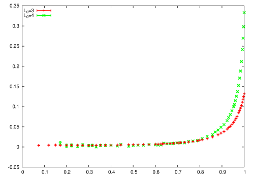
Figure 1: The dependence of $(\langle S[U,{\bf\xi}+a/L_{0}\hat{k}]\rangle-\langle S[U,{\bf\xi}-a/L_{0}\hat{k}]\rangle)/g_{0}^{2}$ on the bare coupling $g_{0}^{2}$. The data have been produced for $L_{0}=3$ and $L_{0}=4$ with shift ${\bf\xi}=(1,0,0)$.

In figure 2 we show the dependence of $\langle T_{0k}\rangle$ on $g_{0}^{2}$; the data have been normalized by $|d_{0}|$, where $d_{0}$ is the value of $\langle T_{0k}\rangle$ at $g_{0}^{2}=0$ and it has been computed analytically [4].

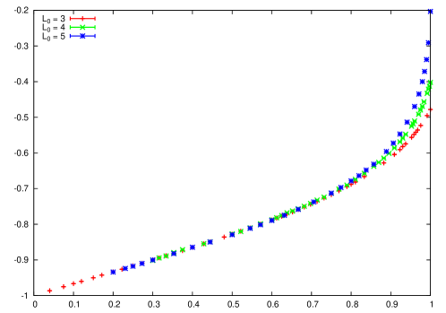
Figure 2: The dependence of $\langle T_{0k}\rangle$ on the bare coupling $g_{0}^{2}$ for $L_{0}=3,4$ and 5. The data are normalized by $|d_{0}|$, where $d_{0}$ is the value of $\langle T_{0k}\rangle$ at $g_{0}^{2}=0$. The value of the shift is ${\bf\xi}=(1,0,0)$.

The integral of eq. (14) is performed by numerical integration and then, by taking the ratio with $\langle T_{0k}\rangle$, one can obtain the dependence of $Z_{T}(g_{0}^{2})$ on $g_{0}^{2}$. The data are shifted by $-c_{0}/d_{0}+1$ in order to reduce the corrections in $a/L$ and $a/L_{0}$. The results are plotted in figure 3 and show almost no dependence on $L_{0}$; also the discretization effects in $L$ are smaller than the statistical errors.

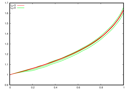
Figure 3: The renormalization factor $Z_{T}(g_{0}^{2})$ of the off-diagonal components of the energy-momentum tensor as a function of the bare coupling $g_{0}^{2}$. The red and green data correspond to $L_{0}=3$ and 4, respectively.

In order to have a check of the reliability of the method, we have performed the above described calculation of $Z_{T}(g_{0}^{2})$ on a lattice with spatial size $L=16$ and $L_{0}=3$. These data – shown using the red and green lines in figure 4 – can be directly compared with those produced at $L=16$ using eq. (13) which are plotted with the black symbols. The cyan and purple symbols correspond to data still obtained with eq. (13) at $L=16$ but with $L_{0}=5$ and 6, respectively. These two sets show that the dependence on $a/L_{0}$ is not visible within the numerical accuracy. Finally, as a further check, we have computed the perturbative expansion of $Z_{T}(g_{0}^{2})$ at two loops using the method of Numerical Stochastic Perturbation Theory [13] at $L=24$ and 48. These latter results, show evidence both for strong finite size effects and for large corrections due to high-order terms and to non-perturbative contributions.

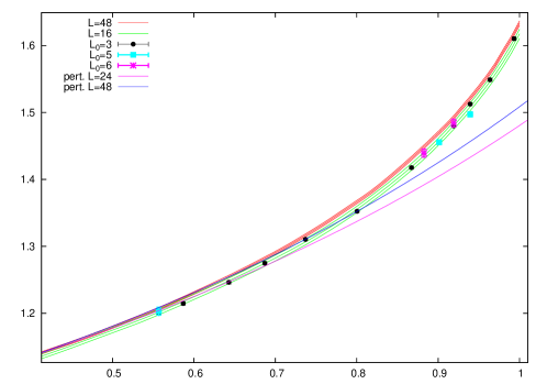
Figure 4: Comparison of different methods to compute the renormalization factor $Z_{T}(g_{0}^{2})$ as a function of the bare coupling $g_{0}^{2}$. The red and green curves are generated using eq. (14) on lattices with spatial size $L=48$ and 16, respectively, and temporal size $L_{0}=3$. The black, cyan and purple symbols are produced using eq. (13) at $L=16$ and $L_{0}=3$, 5 and 6 respectively. The two-loop perturbative expansion are shown in pink and blue for $L=24$ and 48.

4 Conclusions

In this talk we have presented preliminary results for the computation of the renormalization factor of the energy-momentum tensor in $SU(3)$ Yang-Mills theory. We propose a method that allows to attain an accuracy of a few permille in a broad range of values of the bare coupling $g_{0}^{2}$, between 0 and 1 with a moderate numerical effort. The calculation of the renormalization factor is an important input for extracting physically relevant information from the energy-momentum tensor in a Monte Carlo simulation on the lattice.

References

- [1] L. Landau and E. Lifshitz, Course of Theoretical Physics VI: Fluid Mechanics, Butterworth-Heinemann (1987).
- [2] S. Caracciolo, G. Curci, P. Menotti and A. Pelissetto, Annals Phys. 197, 119 (1990).
- [3] L. Giusti and H. B. Meyer, Phys. Rev. Lett. 106, 131601 (2011).
- [4] L. Giusti and H. B. Meyer, JHEP 1301, 140 (2013).
- [5] M. Luscher, Commun. Math. Phys. 293, 899 (2010) [arXiv:0907.5491 [hep-lat]].
- [6] H. Suzuki, PTEP 2013, no. 8, 083B03 (2013).
- [7] L. Del Debbio, A. Patella and A. Rago, JHEP 1311 (2013) 212.
- [8] D. Robaina and H. B. Meyer, Pos (Lattice 2013) 323
- [9] S. Caracciolo, P. Menotti and A. Pelissetto, Phys. Lett. B 260, 401 (1991).
- [10] L. Giusti and M. Pepe, Phys. Rev. Lett. 113, 031601 (2014).
- [11] P. de Forcrand, M. D’Elia and M. Pepe, Phys. Rev. Lett. 86, 1438 (2001).
- [12] M. Della Morte and L. Giusti, Comput. Phys. Commun. 180, 819 (2009).
- [13] F. Di Renzo, E. Onofri, G. Marchesini and P. Marenzoni, Nucl. Phys. B 426, 675 (1994).