Autocorrelation analysis for the unbiased determination of power-law exponents in single-quantum-dot blinking

Abstract

We present an unbiased and robust analysis method for power-law blinking statistics in the photoluminescence of single nano-emitters, allowing us to extract both the bright- and dark-state power-law exponents from the emitters’ intensity autocorrelation functions. As opposed to the widely-used threshold method, our technique therefore does not require discriminating the emission levels of bright and dark states in the experimental intensity timetraces. We rely on the simultaneous recording of 450 emission timetraces of single CdSe/CdS core/shell quantum dots at a frame rate of 250 Hz with single photon sensitivity. Under these conditions, our approach can determine ON and OFF power-law exponents with a precision of 3 % from a comparison to numerical simulations, even for shot-noise-dominated emission signals with an average intensity below 1 photon per frame and per quantum dot. These capabilities pave the way for the unbiased, threshold-free determination of blinking power-law exponents at the micro-second timescale.

Blinking, that is to say intermittent fluorescence ^{1, 2, 3, 4}, is a ubiquitous feature of the emission of nanoparticles ⁵ and can have dramatic consequences for many potential applications. For colloidal quantum dots (QDs), blinking affects the performance of lasers ⁶, light emitting diodes ⁷ and single photon sources ^{8, 9}, to name but a few examples. Photoluminescence (PL) intermittence manifests itself as intensity fluctuations in the fluorescence timetrace of nano-emitters, where highly-emitting states (ON states) are repeatedly interrupted by poorly-emitting states (OFF states). The durations of these alternating ON and OFF periods are found to be distributed according to power laws for many kinds of quantum emitters ⁵, including CdSe/CdS QDs. Under these distributions, the probability $P_{\text{\tiny ON}}(t)\,dt$ of observing an ON state duration between $t$ and $t+dt$ is governed by the probability density

$$P_{\text{\tiny ON}}(t)=(m_{\text{\tiny ON}}-1)\cdot\theta^{m_{\text{ON}}-1}\cdot t^{-m_{\text{ON}}}\qquad,$$ (1)

where $m_{\text{\tiny ON}}$ is the power-law exponent associated with the ON state and $\theta$ is the cut-on time of the blinking process. The expression for the OFF-state probability density $P_{\text{\tiny OFF}}(t)$ can be obtained from Eq. (1) by replacing $m_{\text{\tiny ON}}$ with $m_{\text{\tiny OFF}}$, the corresponding exponent for the OFF state. For colloidal QDs, power law exponents $\lesssim 2$ have been found, which implies non-ergodicity of the ON- and OFF-state dynamics ^{10, 11}.

Theoretical efforts to explain power-law-like emission characteristics started with Randall and Wilkins, who showed that the existence of electron traps with exponentially-distributed depths explains power-law decay of phosphorescence ¹². As far as QDs are concerned, their OFF states are linked to charge separation and electron trapping ¹³, meaning that similar considerations can be applied. Power-law distributed ON times, on the other hand, are less straightforward to account for. More elaborate models have therefore been developed, based on spectral diffusion ^{4, 14}, fluctuating barriers ^{15, 16}, the existence of charged ON states ¹⁷, spatial diffusion ¹⁸, and variations of non-radiative rates ¹⁹. However, while each of these models reproduces a large part of the available experimental evidence, there is still no unified approach that explains all observed properties of QD fluorescence intermittency; as a further complication, the existing models predict different power-law exponents. Recent experimental results have furthermore hinted at the possibility of subtle variations of the exponents when changing parameters like the excitation wavelength ²⁰ or the excitation power ^{21, 22}. As a consequence, an accurate and reliable method to determine power-law exponents from experimental data appears to be crucial for all further efforts toward a unified understanding of the underlying physical phenomena.

Several sophisticated methods exist for the analysis of single-nano-emitter blinking ²³. Studies of power-law blinking usually proceed by first identifying the ON and OFF periods in single-particle fluorescence timetraces and then adjusting Eq. (1) to the probability densities of the observed ON and OFF times ^{3, 4, 15, 24}. The standard procedure of least-squares fitting is known to have problems with long-tailed distributions ²⁵. Thus, more suitable methods to extract $m_{\text{\tiny ON(OFF)}}$ have been developed, based on maximum-likelihood criteria and other statistical tests ^{25, 26, 27, 28}. Nevertheless, all these approaches still crucially depend on a reliable distinction between ON and OFF in the emission intensity traces, which involves establishing an acceptable intensity threshold for a binned timetrace. The nano-emitter is thus considered to be in the ON-state if the intensity of a time bin surpasses this threshold and to be in the OFF-state otherwise, which is straightforward in both concept and implementation. However, it has been shown recently ²⁹ that the extracted $m_{\text{\tiny ON}}$ and $m_{\text{\tiny OFF}}$ can differ by up to $30\%$, depending on the experimental resolution (bin time) and the chosen threshold value. Furthermore, this method obviously depends on the signal-to-noise ratio (SNR) and thus breaks down when the signals are dominated by shot noise, which blurs the distinction between ON and OFF levels and thus limits the temporal resolution that can be achieved.

The change-point detection approach of Watkins et al. ³⁰ is an alternative to the threshold method: Here, the arrival time of every photon is recorded with high temporal resolution ($\sim 100$ ns); a subsequent maximum-likelihood analysis can then identify the most probable times at which ON$\leftrightarrow$OFF transitions occurred. The bin-time bias is thus eliminated as the technique makes the best possible use of the temporal resolution of the data-acquisition electronics. However, a trade-off still exists between efficiency (detecting all state changes, avoiding false negatives) and purity (detecting only “real” state changes, avoiding false positives). This constraint reintroduces a user-biased choice for the acceptable level of false positives, with a concomitant trade-off for false negatives, in the maximum-likelihood analysis.

Two approaches have been explored for extracting $m_{\text{\tiny ON}}$ and $m_{\text{\tiny OFF}}$ power-law blinking exponents without trying to differentiate ON and OFF states explicitly in the timetrace ^{31, 32}. These methods successfully recover the power-law exponent if only one power-law process is at work, but become ambiguous as soon as two such distributions are involved, as is the case for QD blinking. Pelton et al. ³² have analyzed the power spectrum of an ensemble of QDs to show that the Fourier transform of their emission timetrace behaves as $1/f^{\beta}$, where $\beta$ contains the information on both ON and OFF time periods; so far it has not been possible to disentangle the individual contributions of $m_{\text{\tiny ON}}$ and $m_{\text{\tiny OFF}}$.

Verberk et al. ³¹ present an analysis based on the fluorescence intensity autocorrelation function, which makes use of the full information contained in the delays between all pairs of detected photons. As such, it is less sensitive to noise, can be applied to the data at full temporal resolution, and does not require any ON/OFF intensity threshold to be defined. However, the autocorrelation function contains an intermixed information on $m_{\text{\tiny ON}}$ and $m_{\text{\tiny OFF}}$; so far no general analytical expression to extract $m_{\text{\tiny ON}}$ and $m_{\text{\tiny OFF}}$ from the autocorrelation function has been put forward.

In this letter, we present the unbiased determination of $m_{\text{\tiny ON}}$ and $m_{\text{\tiny OFF}}$ power-law blinking exponents of CdSe/CdS QDs using the autocorrelation function. Our approach is robust with respect to experimental noise and temporal resolution, allowing the extraction of power-law exponents from fast ($2$ ms integration time), low-signal ($<1$ photon per frame for each QD on average) blinking data. The method, which we here apply to the PL of single CdSe/CdS quantum dots, does not require setting an intensity threshold for distinguishing ON and OFF states in the experimental emission timetrace, thus removing the potential bias ²⁹ inherent in making such a choice. Furthermore, our technique can easily be extended to photophysical schemes that involve more than two states and we therefore expect it to be applicable to many different types of nano-emitters.

The fact that power-law blinking lacks a typical timescale has dramatic consequences: To obtain complete information on the fluorescence dynamics of single nano-emitters, the total experimental time needs to be infinite. As a consequence, experimental autocorrelation functions, even of one and the same nano-emitter, recorded at different times can deviate from each other significantly. This is not necessarily due to any change in the blinking behavior (the underlying power-law exponents themselves), but rather an intrinsic signature of the non-ergodicity (statistical aging) of luminescence that is governed by power-laws ^{10, 11}. We therefore record a large number of single QD fluorescence timetraces simultaneously so that we can perform a statistical analysis of the corresponding autocorrelation functions; a subsequent comparison to numerical simulations identifies the best-fit power-law exponents with high specificity.

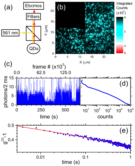
Figure 1: (a) Scheme of the experimental setup. Single QDs are excited at 561 nm with a continuous-wave laser. Photoluminescence is collected through the excitation objective and directed onto the ebCMOS camera. Scattered laser light is suppressed by long-pass filters. (b) Position-dependent integrated photon counts per pixel on a false-color scale; the total acquisition time was 660 s. (The black square in the top left is due to one of the 4 camera quadrants having been turned off during the measurement.) (c) An example of a single QD timetrace extracted from (b). (d) Distribution of the counts of the QD timetrace: no global threshold can be established to discriminate between the ON and OFF states at full temporal resolution (2 ms). (e) Autocorrelation function of the data in (c) (blue dots) and the corresponding fit of Eq. (3) (red line) with parameters $A=0.37$, $B=0.047$ and $C=0.049$.

The experimental setup used to record the timetraces is a home-built wide-field microscope coupled to a high-frame-rate ebCMOS camera ^{33, 34, 35} with high fidelity single photon counting capabilities, see Fig. 1 a. The CdSe/CdS core (3 nm)/shell(8 nm) QDs have an emission maximum centered at 597 nm and spin-coated onto a glass slide from a 90/10 hexane/octane solution. QD luminescence is excited by a 561 nm solid state laser with an intensity of 200 W/cm² in the center of the laser spot. The emission of individual QDs is collected by a $60\times$, $NA=1.35$ oil-immersion objective and is redirected onto the ebCMOS camera with a plano-convex lens of 1 m focal length, resulting in $333\times$ magnification. The overall detection efficiency of the apparatus is around 3%. (Further details on the setup and the QD samples are available in the Supporting Information, Sections 1 and 2.)

We have recorded the fluorescence of 450 single QDs simultaneously at a frame rate of $250$ Hz with a total integration time of 660 seconds. It is worth mentioning that this frame rate is achieved on the full ebCMOS camera chip of $800\times 800$ pixels. To our knowledge, this is the first report of such a large number of single QD timetraces recorded simultaneously at such a high frame rate and with the single photon sensitivity. To validate our method beyond standard conditions (slow acquisition and relatively high SNR), we deliberately kept the excitation power to a minimum, resulting in single-QD timetraces with average count rates of $\sim 1$ photon per frame. Such low-level signals can be recorded with the ebCMOS sensor thanks to its ultra-small dark noise of less than $0.02$ photons/QD/frame on average (see Supporting Information, Fig. S9). Fig. 1 b shows the integrated image of the emission of 450 individual QDs, to which a pattern recognition algorithm was applied to locate the positions of the QDs (see Supporting Information, Section 3). The signal of each QD is then extracted from the sequence of images as a $165\,000$-frame timetrace, an example of which is shown in Fig. 1 c. As can be seen in Fig. 1 d, the distribution of photon counts as commonly used in threshold-based methods ^{25, 26, 27, 28} does not allow for the discrimination between ON and OFF states.

To analyze the single-QD timetraces, their fluorescence intensity autocorrelation functions $g^{(2)}(\tau)$ are calculated according to:

$$g^{(2)}(\tau)=\frac{\bigl{\langle}I(t)\,I(t+\tau)\bigr{\rangle}}{\bigl{\langle}I(t)\bigr{\rangle}^{2}}\qquad,$$ (2)

where $I(t)$ is the intensity (counts per timebin) at time $t$ and $\bigl{\langle}\cdot\bigr{\rangle}$ represents time averages; Fig. 1 e shows an example of a single-QD autocorrelation function. Power-law blinking with exponents $m<2$ lead to timetraces that are dominated by long events whose duration is of the same order of magnitude as the total measurement time ³⁶. As a consequence, the normalization factor $\langle I(t)\rangle^{2}$ in Eq. (2) does not tend toward a well-defined long-time limit. The experimental autocorrelation functions therefore show significant variation from one QD to the next, and even if one and the same QD is probed several times under identical experimental conditions. Nonetheless, the autocorrelation functions exhibit a well-defined general shape for almost all (more than 95%) of the 450 QDs we studied: a power-law decay modulated by an exponential cut-off, in accordance with earlier reports ³¹. The red line in Fig. 1 e shows a fit of the autocorrelation with the following equation:

$$f(t)=A\,t^{-C}\,\exp\bigl{(}-Bt\bigr{)}\quad,$$ (3)

where $A$ represents the autocorrelation contrast, $B$ the cut-off time and $C$ is the power-law exponent of the autocorrelation function; $C$ is equal to $2-m$ if only one of the two states has lifetimes governed by a power law with exponent $m$^{31, 36}. Generally speaking, the decay of an autocorrelation function represents a loss of information about the state of the emitter: As time progresses, it becomes increasingly likely that transitions occur, and at long times one can only make general statistical predictions that are independent of the emitter’s state at time $t=0$. We can therefore surmise that the fit parameter $C$ will be linked to the combined contributions of the $m_{\text{\tiny ON}}$ and $m_{\text{\tiny OFF}}$ distributions, given that both types of transitions are stochastic in nature and hence lead to information loss. The autocorrelation contrast $A$ is influenced by the relative duration of the ON/OFF periods ²³; traces dominated by long OFF periods have higher correlation contrasts than those of an emitter that is mostly in the ON state. The exponential cut-off rate given by parameter $B$, a phenomenological addition to the fit function ³¹, may be attributable, at least partially, to the finite measurement time.

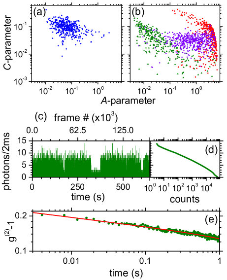
Figure 2: (a) 2D distribution of the $(A,C)$ couples resulting from fitting Eq. (3) to the experimental autocorrelation functions. Our analysis relies on reproducing this 2D distribution with simulated power-law blinking timetraces that are subjected to the same autocorrelation analysis. (b) Three different $(A,C)$ distributions obtained after fitting the autocorrelation functions of simulated traces for three different sets of ($m_{\text{\tiny ON}},m_{\text{\tiny OFF}}$) exponents. Green triangles corresponds to $(1.5,1.7)$, violet squares to $(1.7,1.7)$ and red dots to $(1.7,1.5)$. Every pair of exponents generates its own 2D distribution in the $(A,C)$ space. (c) Example of a simulated timetrace with $(m_{\text{\tiny ON}}=1.80,m_{\text{\tiny OFF}}=1.95)$ power-law exponents. (d) Distribution of the photon counts of the timetrace in (c). As for the experimental data, no global threshold can be established for discriminating ON and OFF states. (e) The corresponding autocorrelation, fitted (red line) by Eq. (3) with adjusted parameters $A=0.13$, $B=0.056$ and $C=0.079$.

Based on the above heuristic arguments, we conclude that the combination of parameters $C$ and $A$ may contain sufficient information to unravel the contributions of $m_{\text{\tiny ON}}$ and $m_{\text{\tiny OFF}}$, even in the absence of a general analytical formula relating the fit parameters to the power-law exponents. (The cut-off parameter $B$ serves as a consistency check, see Supporting Information, Section 8.) Due to the non-ergodicity of power-law blinking, we expect to find a broad distribution of the two parameters in $(A,C)$ space; Fig. 2 a shows that this is indeed the case for the 450 experimental autocorrelation functions. The assumption at the heart of our subsequent analysis is that this 2D distribution of the $(A,C)$ parameters corresponds to one and only one ($m_{\text{\tiny ON}},m_{\text{\tiny OFF}}$) pair of blinking exponents. To validate this assumption, we have simulated 450 single QD timetraces with ON and OFF periods distributed according to power laws with exponents $(m_{\text{\tiny ON}},m_{\text{\tiny OFF}})$ (further details of the simulations and the fitting procedure are given in the Supporting Information, Sections 4 to 7). Fig. 2 c shows an example of a simulated timetrace for $(m_{\text{\tiny ON}},m_{\text{\tiny OFF}})=(1.8,1.95)$ and Fig. 2 e presents the corresponding autocorrelation. For every $(m_{\text{\tiny ON}},m_{\text{\tiny OFF}})$ couple, the 450 simulated autocorrelation functions are fitted with Eq. (3), yielding the 2D distribution of $A$ and $C$ in each case.

Figure 3: (a) Low-resolution comparison of simulations to experimental data with a 2D Kolmogorov-Smirnov (K-S) test. The K-S parameter $D$ (color scale) is represented as a function of the $m_{\text{\tiny ON}}$ and $m_{\text{\tiny OFF}}$ exponents used in the simulations. There is a single $(m_{\text{\tiny ON}},m_{\text{\tiny OFF}})$ couple, $(1.80,1.95)$, that minimizes the $D$-parameter, corresponding to the best agreement between experimental and simulated $(A,C)$ distributions. (b) Same comparison as in (a), now with a simulated set for $(m_{\text{\tiny ON}}=1.80,m_{\text{\tiny OFF}}=1.95)$ replacing the experimental data; all features of the original contour plot (a) are reproduced. (c) High-resolution exploration of the area of minimal $D$ from (a), yielding more accurate optimum values of $(m_{\text{\tiny ON}}=1.805,m_{\text{\tiny OFF}}=1.955)$ $\pm 3$%. (d) 2D distributions of $A$ and $C$ for the data (blue dots, same as in Fig. 2 a) and the best-fit simulation $(m_{\text{\tiny ON}}=1.805,m_{\text{\tiny OFF}}=1.955)$ (red triangles). (e) Reproducibility and distinctiveness of $D$: The red histogram shows the distribution found for $D$ when comparing the experimental $(A,C)$ distribution to 215 different analysis runs for the previously-determined optimum couple $(m_{\text{\tiny ON}}=1.805,m_{\text{\tiny OFF}}=1.955)$, while the black bars represent the analogous distribution for $(m_{\text{\tiny ON}}=1.85,m_{\text{\tiny OFF}}=2.00)$, the second-lowest pixel in the contour plot in (a). The green histogram corresponds to a null-hypothesis calibration, for which one simulation run for $(m_{\text{\tiny ON}}=1.805,m_{\text{\tiny OFF}}=1.955)$ is compared to 215 additional runs for the very same pair of parameters.

Three examples of such simulated distributions are plotted in Fig. 2 b for $(m_{\text{\tiny ON}},m_{\text{\tiny OFF}})=(1.5,1.7)$, $(1.7,1.7)$ and $(1.7,1.5)$. As expected, the distributions for each $(m_{\text{\tiny ON}},m_{\text{\tiny OFF}})$ pair are spread over a large area in $(A,C)$ space, meaning that correctly identifying the underlying power-law exponents requires studying a statistically significant number of single QDs (see Supporting Information, Section 13). Given a large-enough data set, we can test whether a single $(m_{\text{\tiny ON}},m_{\text{\tiny OFF}})$ couple can be identified as the ”best fit“ for describing the experimental data of Fig. 2 a. To this end, we use a 2D Kolmogorov-Smirnov (K-S) statistical test ^{37, 38}, which compares the 2D $(A,C)$ distributions of two different data sets, yielding a parameter $D$ that quantifies the mismatch between the two distributions: $D\in[0,1]$, where $D=0$ would correspond to prefect overlap. In total, we have tested 1444 different $(m_{\text{\tiny ON}},m_{\text{\tiny OFF}})$ combinations ranging from $(1.05,1.05)$ to $(2.9,2.9)$, covering more than the spread of values reported in the literature ^{26, 20, 5, 39, 40, 28}. That is to say, we have simulated 450 single-QD timetraces for each $(m_{\text{\tiny ON}},m_{\text{\tiny OFF}})$ couple, determined the corresponding 2D distribution in $(A,C)$ space and calculated the K-S parameter $D$ with respect to the experimental data of Fig. 2 a. The 2D contour plot in Fig. 3 a shows the resulting values of $D$ on a color scale as a function of $m_{\text{\tiny ON}}$ and $m_{\text{\tiny OFF}}$; the high contrast of $D$ spans variations of one order of magnitude, from $D\simeq 0.1$ to $1$. There is an isolated, well-defined minimum of $D\lesssim 0.1$ at $(1.8,1.95)$, indicating that a singular, narrowly-delimited combination of exponents optimizes the overlap between the experimental data and simulations based on the power-law model of Eq. (1). A high-resolution contour plot of the parameter space around the minimum of $D$ can be seen in Fig. 3 c. For this particular ensemble of CdSe/CdS QDs, we thus find best-fit blinking exponents of $(m_{\text{\tiny ON}}=1.805,m_{\text{\tiny OFF}}=1.955)$ for the pixel with minimum $D$; the corresponding simulated $(A,C)$ distribution is compared to the experimental data in Fig. 3 d.

After having shown that our approach can identify the optimal $(m_{\text{\tiny ON}},m_{\text{\tiny OFF}})$ couple with high specificity, we now discuss to what extent the autocorrelation analysis allows us to judge whether the underlying hypothesis itself – QD blinking is governed by power-law distributed probabilities, Eq. (1) – is justified. To explore this issue, we took a simulated data set for $(m_{\text{\tiny ON}}=1.805,m_{\text{\tiny OFF}}=1.955)$, i. e., an ensemble of timetraces for which we know the null hypothesis to be true, and we subjected this set to the same analysis as the experimental data. We can thus identify the behavior of $D$ that corresponds to genuine power-law blinking and quantify the degree of variation in $D$ that is inherent in repeatedly probing the same power-law distributions with limited sample sizes and measurement times. As can be seen in Fig. 3 b, the resulting ”ideal“ contour plot agrees very well with the experimental one of Fig. 3 a, down to the shape of the faint offshoots observed for the main and secondary minima. However, the values of $D$ are slightly lower in the minimum regions of Fig. 3 b, although this is barely noticeable given the color scale. We further investigated this feature by subjecting both the real and the idealized (simulated) data to 215 different analysis runs for the previously identified optimum parameters $(m_{\text{\tiny ON}}=1.805,m_{\text{\tiny OFF}}=1.955)$. Each analysis run is based on a new seed of the random number generator and therefore produces its own simulated $(A,C)$ distribution, to which both data sets (real and idealized) are then compared with the K-S test. The simulation-simulation analyses thus yield the distribution of $D$ values that can be expected for idealized power-law blinking, which, as is shown in Fig. 3 e (green histogram), has its mean value at $D_{\text{sim}}=0.074$ with a standard deviation of $\sigma_{\text{sim}}=0.014$. The experiment-simulation analysis runs, on the other hand, produce a roughly Gaussian-shaped histogram (red) with mean value $D_{\text{exp}}=0.107$ and standard deviation $\sigma_{\text{exp}}=0.013$. There is about 20% overlap between the experiment-simulation and the simulation-simulation distributions, with the $D$ values for the experimental data being larger in general. This means that the data, on average, tends to agree slightly less well with simulations than can be expected from the variations between equivalent simulation-simulation analysis runs. Nevertheless, the large overlap means that there is no reason to reject the null hypothesis at the base of our analysis, which supposed that the blinking behavior of all the investigated QDs can be modeled by a power law with a single $(m_{\text{\tiny ON}},m_{\text{\tiny OFF}})$ combination. The remaining small offset between $D_{\text{exp}}$ and $D_{\text{sim}}$ might be due to an aspect of the particles’ photophysics that is not incorporated in our model. For example, small inhomogeneities may be present in the investigated sample of 450 QDs as far as power-law exponents, the exciton emission rates and/or the ratios between bright and dark state emission efficiencies are concerned.

The black histogram in Fig. 3 e is the result of the experiment-simulation comparison for $(m_{\text{\tiny ON}}=1.85,m_{\text{\tiny OFF}}=2.00)$, which corresponds to the pixel with the second-lowest $D$ in the contour plot of Fig. 3 a. There is strictly no overlap with the $D$ distribution for the optimum fit parameters (red histogram), illustrating once more the specificity of the autocorrelation analysis. In fact, as is detailed in the Supporting Information (Sections 9 and 11), we find that all 8 nearest-neighbor pixels in Fig. 3 a exhibit distributions whose maxima differ by at least $6\sigma$ from the mean value of $D=0.107$ of the optimum-solution histogram (red); where $\sigma$ stands for the largest standard deviation of the compared histograms (worst case scenario). We therefore conclude that we are able to extract the power-law exponents with an absolute precision of $\pm 0.05$ ($\pm 3$%) at $6\sigma$ specificity. The combination of $m_{\text{\tiny ON}}=1.805$ with an almost 10% larger $m_{\text{\tiny OFF}}=1.955$ indicates that these QDs spend most of the time in the ON state under continuous illumination, a typical feature of such large-shell CdSe/CdS QDs ^{39, 41}. It is particularly noteworthy that $m_{\text{\tiny OFF}}$ approaches the critical threshold of $2$, above which the average duration of the OFF periods becomes finite. The power-law exponent of the ON periods, on the other hand, is associated with an infinite average length; overall, this leads to a favorable interplay of ON versus OFF periods in the photoluminescence of this type of QD.

To complete the discussion of our technique, we now address its robustness with respect to two critical factors. First, we consider the influence of the ON/OFF intensity contrast. OFF states can still be moderately emissive (“dim” instead of completely dark), which makes it harder to distinguish them from the ON states. In fact, residual OFF state emission manifests itself in the contour plot of Fig. 3 a, which shows, besides the global minimum of $D=0.1$, as a second domain (green) of relatively low $D$ values around $0.4$. This secondary minimum arises due to the relatively high quantum yield of the dark state for this type of QD, reaching $10$% of the bright state emission. We show in the Supporting Information (Section 15) that this region shifts as a function of the dark state emissivity and tends to vanish if this emissivity drops below $\sim 0.1\%$ of the efficiency of the bright state. With regard to more emissive “dark” states, we verified (see Supporting Information, Section 15) that our technique maintains a precision of $\pm 0.05$ (under the experimental conditions discussed in this work) as long as dark state efficiencies stay below $50$% of the bright states. As a consequence, the approach is also suitable for analyzing recently developed types of giant-shell ^{42, 43, 41} or alloyed QDs ⁴⁴, both of which having a high dark-state-emission efficiency.

The second important benchmark is the interplay between count rate, temporal resolution and residual uncertainty for the power-law exponents, which is linked to the sensitivity of the $D$ parameter. As discussed above, we are able to extract the power-law exponents with an absolute precision of $\pm 0.05$ ($\pm 3$%) at $6\sigma$ specificity. It is worth noting that this precision is achieved with shot-noise-dominated timetraces, well below saturation of the QD emission. Such minimally-invasive conditions are preferable to approaches that require high count rates to discriminate between ON and OFF states, and hence high excitation intensities that may influence the blinking parameters ^{22, 21} and can furthermore lead to photobleaching. As far as the temporal resolution is concerned, our method can extract blinking power-law exponents for timetraces with only 0.1 photons/QD/frame on average, with a reasonable acquisition time $T_{\text{max}}=66$ s with $3\%$ precision ($\pm 0.05$) at $6\sigma$ specificity (see Supporting Information, Section 14). This robustness of our method against noise may allow blinking studies at up to 100 kHz (10 µs resolution), one order of magnitude faster than what has been demonstrated with change-point detection ³⁰. Verifying power-law behavior at the fastest possible timescale will be useful to elucidate the role of the cut-on time, $\theta$ in Eq. (1). Taking a pragmatic point of view, this cut-on time can be equated with the experimental temporal resolution; nevertheless, a more fundamental approach can be expected to improve our understanding of QD photophysics, for example if a timescale can be identified at which the power-law behavior breaks down.

In conclusion, we have presented a technique to determine unbiased power-law exponents of blinking CdSe/CdS core/shell QDs with a precision of 3 % at $6\sigma$ specificity. To our knowledge, this constitutes the first approach for extracting the full set of blinking parameters from experimental autocorrelation functions, bypassing the need of introducing a possibly-biased ON/OFF threshold. Our autocorrelation analysis is robust in the presence of noise and intrinsically free from timebin-dependent thresholding artifacts. As such, the method is capable of determining $m_{\text{\tiny ON}}$ and $m_{\text{\tiny OFF}}$ from timetraces dominated by shot noise, which are untreatable by other methods. We thus can extract the power-law exponents from ultra-low signal data ($\sim 0.1$ photon/frame/QD) with a precision of 3$\%$, which offers the perspective of threshold-free blinking analysis at the micro-second timescale.

Supporting Information Available.

Extensive supporting information on experimental techniques, numerical simulations, and further capability benchmarks of our approach is available free of charge via the Internet at http://pubs.acs.org.

References

- Nirmal et al. 1996 Nirmal, M.; Dabbousi, B. O.; Bawendi, M. G.; Macklin, J. J.; Trautman, J. K.; Harris, T. D.; Brus, L. E. Nature 1996, 383, 802–804
- Banin et al. 1999 Banin, U.; Bruchez, M.; Alivisatos, A. P.; Ha, T.; Weiss, S.; Chemla, D. S. J. Chem. Phys. 1999, 110, 1195–1201
- Kuno et al. 2000 Kuno, M.; Fromm, D. P.; Hamann, H. F.; Gallagher, A.; Nesbitt, D. J. J. Chem. Phys. 2000, 112, 3117–3120
- Shimizu et al. 2001 Shimizu, K. T.; Neuhauser, R. G.; Leatherdale, C. A.; Empedocles, S. A.; Woo, W. K.; Bawendi, M. G. Phys. Rev. B 2001, 63, 205316
- Frantsuzov et al. 2008 Frantsuzov, P.; Kuno, M.; Janko, B.; Marcus, R. A. Nat. Phys. 2008, 4, 519–522
- Klimov et al. 2000 Klimov, V. I.; Mikhailovsky, A. A.; Xu, S.; Malko, A.; Hollingsworth, J. A.; Leatherdale, C. A.; Eisler, H. J.; Bawendi, M. G. Science 2000, 290, 314–317
- Anikeeva et al. 2007 Anikeeva, P. O.; Halpert, J. E.; Bawendi, M. G.; Bulovic, V. Nano Lett. 2007, 7, 2196–2200
- Lounis et al. 2000 Lounis, B.; Bechtel, H. A.; Gerion, D.; Alivisatos, P.; Moerner, W. E. Chem. Phys. Lett. 2000, 329, 399–404
- Michler et al. 2000 Michler, P.; Imamoğlu, A.; Mason, M. D.; Carson, P. J.; Strouse, G. F.; Buratto, S. K. Nature 2000, 406, 968–970
- Brokmann et al. 2003 Brokmann, X.; Hermier, J. P.; Messin, G.; Desbiolles, P.; Bouchaud, J. P.; Dahan, M. Phys. Rev. Lett. 2003, 90, 120601
- Lutz 2004 Lutz, E. Phys. Rev. Lett. 2004, 93, 190602
- Randall and Wilkins 1945 Randall, J. T.; Wilkins, M. H. F. Proc. R. Soc. A-Math. Phys. Eng. Sci. 1945, 184, 390–407
- Efros and Rosen 1997 Efros, A. L.; Rosen, M. Phys. Rev. Lett. 1997, 78, 1110–1113
- Tang and Marcus 2005 Tang, J.; Marcus, R. A. Phys. Rev. Lett. 2005, 95, 107401
- Kuno et al. 2001 Kuno, M.; Fromm, D. P.; Hamann, H. F.; Gallagher, A.; Nesbitt, D. J. J. Chem. Phys. 2001, 115, 1028–1040
- Kuno et al. 2003 Kuno, M.; Fromm, D. P.; Johnson, S. T.; Gallagher, A.; Nesbitt, D. J. Phys. Rev. B 2003, 67, 125304
- Verberk et al. 2002 Verberk, R.; van Oijen, A. M.; Orrit, M. Phys. Rev. B 2002, 66, 233202
- Margolin et al. 2006 Margolin, G.; Protasenko, V.; Kuno, M.; Barkai, E. adv chem phys 2006, 133, 327–356
- Frantsuzov and Marcus 2005 Frantsuzov, P. A.; Marcus, R. A. Phys. Rev. B 2005, 72, 155321
- Knappenberger et al. 2007 Knappenberger, K. L.; Wong, D. B.; Romanyuk, Y. E.; Leone, S. R. Nano Lett. 2007, 7, 3869–3874
- Goushi et al. 2009 Goushi, K.; Yamada, T.; Otomo, A. J. Phys. Chem. C 2009, 113, 20161–20168
- Malko et al. 2011 Malko, A. V.; Park, Y. S.; Sampat, S.; Galland, C.; Vela, J.; Chen, Y. F.; Hollingsworth, J. A.; Klimov, V. I.; Htoon, H. Nano Lett. 2011, 11, 5213–5218
- Lippitz et al. 2005 Lippitz, M.; Kulzer, F.; Orrit, M. ChemPhysChem 2005, 6, 770–789
- Sher et al. 2008 Sher, P. H.; Smith, J. M.; Dalgarno, P. A.; Warburton, R. J.; Chen, X.; Dobson, P. J.; Daniels, S. M.; Pickett, N. L.; O’Brien, P. Appl. Phys. Lett. 2008, 92, 101111
- Goldstein et al. 2004 Goldstein, M. L.; Morris, S. A.; Yen, G. G. Eur. Phys. J. B 2004, 41, 255–258
- Hoogenboom et al. 2006 Hoogenboom, J. P.; den Otter, W. K.; Offerhaus, H. L. J. Chem. Phys. 2006, 125, 204713
- Clauset et al. 2009 Clauset, A.; Shalizi, C. R.; Newman, M. E. J. SIAM Rev. 2009, 51, 661–703
- Riley et al. 2012 Riley, E. A.; Hess, C. M.; Whitham, P. J.; Reid, P. J. J. Chem. Phys. 2012, 136, 184508
- Crouch et al. 2010 Crouch, C. H.; Sauter, O.; Wu, X. H.; Purcell, R.; Querner, C.; Drndic, M.; Pelton, M. Nano Lett. 2010, 10, 1692–1698
- Watkins and Yang 2005 Watkins, L. P.; Yang, H. J. Phys. Chem. B 2005, 109, 617–628
- Verberk and Orrit 2003 Verberk, R.; Orrit, M. J. Chem. Phys. 2003, 119, 2214–2222
- Pelton et al. 2004 Pelton, M.; Grier, D. G.; Guyot-Sionnest, P. Appl. Phys. Lett. 2004, 85, 819–821
- Barbier et al. 2011 Barbier, R. et al. Nucl. Instrum. Methods Phys. Res. Sect. A-Accel. Spectrom. Dect. Assoc.Equip. 2011, 648, 266–274
- Doan et al. 2012 Doan, Q.; Barbier, R.; Dominjon, A.; Cajgfinger, T.; Guérin, C. Proc. SPIE 2012, 8436, 84360J
- Guérin et al. 2012 Guérin, C.; Mahroug, J.; Tromeur, W.; Houles, J.; Calabria, P.; Barbier, R. Nucl. Instrum. Methods Phys. Res. Sect. A-Accel. Spectrom. Dect. Assoc.Equip. 2012, 695, 420–424
- Bardou et al. 2002 Bardou, F.; Bouchaud, J.-P.; Aspect, A.; Cohen-Tannoudji, C. Lévy Statistics and Laser Cooling: How Rare Events Bring Atoms to Rest; Cambridge University Press: Cambridge, 2002
- Peacock 1983 Peacock, J. A. Mon. Not. Roy. Astron. Soc. 1983, 202, 615–627
- Fasano and Franceschini 1987 Fasano, G.; Franceschini, A. Mon. Not. Roy. Astron. Soc. 1987, 225, 155–170
- Mahler et al. 2008 Mahler, B.; Spinicelli, P.; Buil, S.; Quélin, X.; Hermier, J. P.; Dubertret, B. Nat. Mater. 2008, 7, 659–664
- Orrit 2010 Orrit, M. Photochem. Photobiol. Sci. 2010, 9, 637–642
- Canneson et al. 2014 Canneson, D.; Biadala, L.; Buil, S.; Quélin, X.; Javaux, C.; Dubertret, B.; Hermier, J. P. Phys. Rev. B 2014, 89, 035303
- Galland et al. 2013 Galland, C.; Brovelli, S.; Bae, W. K.; Padilha, L. A.; Meinardi, F.; Klimov, V. I. Nano Lett. 2013, 13, 321–328
- Javaux et al. 2013 Javaux, C.; Mahler, B.; Dubertret, B.; Shabaev, A.; Rodina, A. V.; Efros, A. L.; Yakovlev, D. R.; Liu, F.; Bayer, M.; Camps, G.; Biadala, L.; Buil, S.; Quélin, X.; Hermier, J. P. Nat. Nanotechnol. 2013, 8, 206–212
- Wang et al. 2009 Wang, X. Y.; Ren, X. F.; Kahen, K.; Hahn, M. A.; Rajeswaran, M.; Maccagnano-Zacher, S.; Silcox, J.; Cragg, G. E.; Efros, A. L.; Krauss, T. D. Nature 2009, 459, 686–689