Velocity Induced Neutrino Oscillation and its Possible Implications for Long Baseline Neutrinos

Abstract

If the three types of active neutrinos possess different maximum attainable velocities and the neutrino eigenstates in the velocity basis are different from those in the flavour (and mass) basis then this will induce a flavour oscillation in addition to the normal mass flavour oscillation. Here we study such an oscillation scenario in three neutrino framework including also the matter effect and apply our results to demonstrate its consequences for long baseline neutrinos. We also predict the possible signatures in terms of yields in a possible long baseline neutrino experiment.

PACS Nos.: 14.60.Pq

1 Introduction

It is now established that neutrinos exhibit the phenomenon of oscillation whereby one type of neutrino (electron, muon or tau) can change to another flavour when they propagate through vacuum or matter. It is also established that they are massive and the fact that their mass eigenstates and their weak interaction eigenstates are not same, leads to the phenomenon of oscillation. The origin of mass for the neutrinos cannot be explained within the framework of Standard Model of particle physics and one may need theories beyond Standard Model (SM) to explain how neutrinos acquire mass. Thus neutrinos provide us an window for new physics beyond SM. Moreover, neutrino can play a key role in addressing the CP violation in leptonic sector. The neutrinos, if Majorana fermions, could be a useful probe to address the problem of leptogenesis and explain the phenomenon of neutrinoless double beta decay.

The oscillation in neutrinos can also be introduced in other exotic scenarios such as violation of equivalence principle (VEP) whereby three types of neutrinos interact gravitationally with different strengths and thus their eigenstates in gravity basis is not the same as those in interaction basis. This scenario has been explored in some previous works [1, 2, 3]. Neutrino flavour oscillations, other than mass-flavour oscillation, can also be initiated if three different neutrinos have different maximum attainable velocities. This may be possible when the three massive neutrinos have different masses. In this scenario the mixing between the flavour and velocity eigenstates can induce neutrino flavour oscillation. It is to be noted that while the oscillation length $\lambda\sim E_{\nu}$ ($E_{\nu}$ is the neutrino energy) for ordinary mass-flavour oscillation, for the cases of both velocity induced flavour oscillation and VEP induced oscillation, $\lambda\sim\frac{1}{E_{\nu}}$. In fact, for velocity induced oscillation, $\lambda=\frac{2\pi}{E_{\nu}\Delta V}$ where $\Delta V$ is the difference in maximum attainable velocities of two neutrinos. In case of mass-flavour oscillation $\lambda=\frac{4\pi E_{\nu}}{\Delta m^{2}}$, where $\Delta m^{2}$ is the mass square difference between two neutrinos.

Studies of velocity induced neutrino oscillation have been performed by previous authors [4], where they consider the violation of Lorentz invariance whereby one of the neutrinos may acquire velocity higher than $c$, the velocity of light. Detailed study on the prospect of velocity induced oscillation in two flavour scenario is given in Coleman and Glashow[4]. Such study, with experimental data considering $\nu_{\mu}\rightarrow\nu_{e}$ maximal mixing, predicts that $\Delta V<10^{-21}$. There are other works too, where this issue has been addressed. Fogli et al[5] has made an analysis of atmospheric neutrino data from Super-Kamiokande experiment for both the velocity induced and VEP induced oscillations and obtained a bound $\Delta V<10^{-24}$. In a later work by Battistoni et al [6], the data of upward going muons for atmospheric neutrinos in MACRO experiment[7, 8] has been analysed considering both mass flavour oscillation and velocity induced oscillation. This analysis gave a bound (with 90% C.L.) as $\Delta V<6\times 10^{-24}$ for the velocity-flavour state mixing angle $\theta_{v}=0$ and $\Delta V<(2.5-5)\times 10^{-26}$ for $\theta_{v}=\frac{\pi}{4}$. But in both the analyses above, only 2-flavour oscillation, $\nu_{\mu}\rightarrow\nu_{\tau}$, is considered. The matter effect on neutrino oscillation is irrelevant for only $\nu_{\mu}\rightarrow\nu_{\tau}$ oscillation scenario (since the matter effect term is same for both $\nu_{\mu}$ and $\nu_{\tau}$, no phase difference can be generated). Thus both analyses are for vacuum oscillation only. In a more recent work [9], it is shown from the analysis of atmospheric and long baseline neutrino (LBL) data that the bound on $\Delta V$ for $\nu_{\mu}\rightarrow\nu_{\tau}$ oscillation with CPT even effects is $\leq 10^{-24}$.

In this work we consider three types of neutrinos having different velocities such that their velocity eigenstates differ from their flavour eigenstates and mass eigenstates. We investigate the combined oscillation phenomenology for both mass-flavour and velocity flavour oscillations. We explore how the velocity induced oscillation changes when the matter effect is included. As discussed earlier, in this scenario, the oscillation depends both on the difference of velocities $\Delta V$ of any two neutrinos. We investigate the possible magnitudes for $\Delta V$ in order that this velocity-driven oscillation (with $\Delta m^{2}$) can have significant effects in the combined oscillation scenario (mass induced and velocity induced oscillation with matter effect) mentioned above. Our formalism is then applied to demonstrate the nature of this velocity induced oscillation for three massive neutrinos with and without the matter effect for a chosen baseline through earth matter. We then compute the number of neutrino induced muons for such a scenario in case of a possible long baseline experiment with an iron calorimeter (ICAL) as the end detector.

The paper is organised as follows. In Section 2 we give the general framework for neutrino oscillation formalism of massive induced by the velocity eigenstates of neutrinos including the matter effect, as also for the case where matter effect is not included. The possible signature of such velocity induced oscillation in a long baseline experiment is probed considering a specific example for demonstrative purpose. This is given in Sect. 3. Finally in Sect. 4 we make some concluding remarks.

2 Neutrino Oscillation Framework with Velocity Eigenstates

The basic idea of neutrino oscillation, first given by Pontecorvo [10, 11], comes from simple quantum mechanics of a two - level quantum system. Let the system be in one of its stationary states. Let an eigenstate of its Hamiltonian be expressed as $|\psi_{i}\rangle$ whose time evolution is written as $|\psi_{i}(t)\rangle=e^{-iE_{i}t}|\psi_{i}(0)\rangle$. If a state is produced which is not one of the eigenstates of the Hamiltonian, the probability that the system retains its state will then oscillate with time depending on the frequency $\omega_{21}=E_{2}-E_{1}$, where $E_{1}$ and $E_{2}$ are the energy eigenvalues of the two level quantum system. Since the eigenstates in the mass (energy) basis of a neutrino are not the same as those in interaction or flavour basis, a neutrino produced in certain flavour eigenstate $|\nu_{\alpha}\rangle$ of flavour $\alpha$ can oscillate into other flavour with a definite probability or come back to its initial flavour state as well. The neutrino flavour eigenstates and mass eigenstates are related through a unitary matrix $U$ which can be parametrised as

$$\left(\begin{array}[]{c}|\nu_{e}\rangle\\ |\nu_{\mu}\rangle\\ |\nu_{\tau}\rangle\end{array}\right) = \left(\begin{array}[]{ccc}U_{e1}&U_{e2}&U_{e3}\\ U_{\mu 1}&U_{\mu 2}&U_{\mu 3}\\ U_{\tau 1}&U_{\tau 2}&U_{\tau 3}\end{array}\right)\left(\begin{array}[]{c}|\nu_{1}\rangle\\ |\nu_{2}\rangle\\ |\nu_{3}\rangle\end{array}\right).$$ (10)

Therefore, a flavour eigenstate $|\nu_{\alpha}\rangle$ ($\alpha=e,\mu\,{\rm or}\,\tau$) is related to mass eigenstates $|\nu_{i}\rangle(i=1,2,3)$ by the relation

$$|\nu_{\alpha}\rangle = \sum_{i}U_{\alpha i}|\nu_{i}\rangle\,\,.$$ (11)

Assuming the neutrinos to be CP conserving, the mixing matrix $U$ can be expressed in terms of three orthogonal matrices, $V_{23}$, $V_{13}$ and $V_{12}$ (three successive rotations) as [12, 13]

$$U = V_{23}V_{13}V_{12}$$ (21)

$$= \left(\begin{array}[]{ccc}1&0&0\\ 0&c_{23}&s_{23}\\ 0&-s_{23}&c_{23}\end{array}\right)\left(\begin{array}[]{ccc}c_{23}&0&s_{13}\\ 0&1&0\\ -s_{23}&0&c_{23}\end{array}\right)\left(\begin{array}[]{ccc}c_{12}&s_{12}&0\\ -s_{12}&c_{12}&0\\ 0&0&1\end{array}\right).$$

The mixing matrix $U$ takes the form

$$U = \left(\begin{array}[]{ccc}c_{13}c_{12}&s_{12}c_{13}&s_{13}\\ -s_{12}c_{23}-s_{23}s_{13}c_{12}&c_{23}c_{12}-s_{23}s_{13}s_{12}&s_{23}c_{13}\\ s_{23}s_{12}-s_{13}c_{23}c_{12}&-s_{23}c_{12}-s_{13}s_{12}c_{23}&c_{23}c_{13}\end{array}\right)\,\,.$$ (25)

In Eqs. (21) - (25), $c_{ij}\equiv\cos\Theta_{ij}$ and $s_{ij}\equiv\sin\Theta_{ij}$ and $\Theta_{ij}$ is the flavour mixing angle between $i^{\rm th}$ and $j^{\rm th}$ neutrinos having mass eigenstate $|\nu_{i}\rangle$ and $|\nu_{j}\rangle$ respectively. Needless to mention that $U$ is a unitary matrix.

The time evolution of the neutrinos with mass eigenstate $|\nu_{i}\rangle,\,(i=1,2,3)$ is (in natural units) given by

$$i\frac{d}{dt}\left(\begin{array}[]{c}|\nu_{1}\rangle\\ |\nu_{2}\rangle\\ |\nu_{3}\rangle\end{array}\right) = \left(\begin{array}[]{ccc}E_{1}&0&0\\ 0&E_{2}&0\\ 0&0&E_{3}\end{array}\right)\left(\begin{array}[]{c}|\nu_{1}\rangle\\ |\nu_{2}\rangle\\ |\nu_{3}\rangle\end{array}\right)=H_{d}\left(\begin{array}[]{ccc}|\nu_{1}\rangle\\ |\nu_{2}\rangle\\ |\nu_{3}\rangle\end{array}\right)$$ (38)

Using Eqs. (10), (11), one gets the evolution equation in flavour basis as

$$i\frac{d}{dt}U^{\dagger}\left(\begin{array}[]{c}|\nu_{e}\rangle\\ |\nu_{\mu}\rangle\\ |\nu_{\tau}\rangle\end{array}\right) = H_{d}U^{\dagger}\left(\begin{array}[]{c}|\nu_{e}\rangle\\ |\nu_{\mu}\rangle\\ |\nu_{\tau}\rangle\end{array}\right),$$ (45)

$$i\frac{d}{dt}\left(\begin{array}[]{c}|\nu_{e}\rangle\\ |\nu_{\mu}\rangle\\ |\nu_{\tau}\rangle\end{array}\right) = H\left(\begin{array}[]{c}|\nu_{e}\rangle\\ |\nu_{\mu}\rangle\\ |\nu_{\tau}\rangle\end{array}\right)$$ (52)

where

$$H = UH_{d}U^{\dagger}$$ (53)

In the above, $H_{d}$ is the Hamiltonian in mass basis with the energy and mass eigenvalues of the three neutrinos are denoted as $E_{i},~{}i=1,2,3$ and $m_{i},~{}i=1,2,3$. Now the diagonal matrix $H_{d}$ can be written in the form

$$H_{d} = \left(\begin{array}[]{ccc}E_{1}&0&0\\ 0&E_{2}&0\\ 0&0&E_{3}\end{array}\right)\approx\frac{1}{2E}\left(\begin{array}[]{ccc}m_{1}^{2}&0&0\\ 0&m_{2}^{2}&0\\ 0&0&m^{2}_{3}\end{array}\right)$$ (60)

$$\approx \frac{1}{2E}{\rm diag}(-\Delta m_{21}^{2},0,\Delta m_{32}^{2})\,.$$ (61)

Eq. (7) is obtained with the approximation that the neutrino momenta $p_{i}\approx E_{i}$ ($i=1,2,3$) and $p_{1}\approx p_{2}\approx p_{3}=p\approx E$. Then, $E_{i}=\sqrt{p_{i}^{2}+m_{i}^{2}}\approx p+\frac{m_{i}^{2}}{2p}\approx p+\frac{m_{i}^{2}}{2E}$. In Eq. (61), $\Delta m_{ij}^{2}$ denotes the difference of the square of the masses of $i^{\rm th}$ and $j^{\rm th}$ neutrinos. The matrix $\frac{1}{2E}{\rm diag}(m_{2}^{2},m_{2}^{2},m_{2}^{2})$ which is subtracted from Eq. (7) to obtain Eq. (61) as also the matrix ${\rm diag}({p,p,p})$ which are neglected in Eq. (7) induce no phase difference between any two neutrinos and hence do not contribute to oscillation. The flavour oscillation probability (mass-induced) for a neutrino of flavour $\alpha$ ($|\nu_{\alpha}\rangle$, $\alpha$ denotes $e$ or $\mu$ or $\tau$) after a time $t$ when it traverses a distance $L=ct$, can now be obtained by solving Eq. (52) and calculating the quantity $|\langle\nu_{\alpha}(t)|\nu_{\alpha}(t=0)\rangle|^{2}$ (the square of the ampliude). We mention in the passing that oscillation probability for pure mass-flavour vacuum oscillation considering only two neutrino species is given by

$$P_{12}=\sin^{2}\theta\sin^{2}\left(\frac{\Delta m^{2}_{21}L}{4E}\right),$$

where $\theta$ is the mixing angle between the two active neutrino species. For the case of mass-flavour oscillation, the oscillation probability depends on the phase difference which is $\sim\frac{1}{E}$ (oscillation length $\lambda=\frac{4\pi E}{\Delta m^{2}_{21}}$) and this also holds for the case of oscillation of three active neutrinos.

Massive neutrinos may also exhibit oscillation phenomena if different neutrinos have different maximum attainable velocities and they travel at different speeds in vacuum. As they move with different velocities they must differ in energy. If the velocity eigenstates are not the same as flavour eigenstates then similar to the mass induced oscillation, one has velocity-flavour oscillation induced by different maximum velocities of neutrinos. In such a scenario, the velocity eigenstate $\left|\nu_{V_{i}}\right\rangle,~{}i=1,2,3$ is related to the flavour eigenstate $|\nu_{\alpha}\rangle,~{}\alpha\equiv e,\mu,\tau$ through three mixing angles $\Theta^{{}^{\prime}}_{ij}(i\neq j),~{}i,j=1,2,3$. The difference in velocities between any two species of neutrinos moving with different maximum attainable velocities can be expressed as

$$\Delta V_{ji} = V_{j}-V_{i}=\frac{p_{j}}{E_{j}}-\frac{p_{i}}{E_{i}}\,,$$

$$\Delta V_{ji}E = p_{j}-p_{i}~{};(E_{j}\approx E_{i}\approx E),$$

where $V_{i({\rm or}~{}j)}$, $p_{i({\rm or}~{}j)}$, $E_{i({\rm or}~{}j)}$ respectively denote the maximum attainable velocity, momentum and energy for the neutrino species $|\nu_{i({\rm or}~{}j)}\rangle$. With the approximation that $E_{j}=p_{j}$ and $E_{i}=p_{i}$, in the above equation the energy difference between any two species of neutrinos $|\nu_{j}\rangle$ and $|\nu_{i}\rangle$ is obtained as[4]

$$p_{j}-p_{i}\approx E_{j}-E_{i}=\Delta E_{ji} = \Delta V_{ji}E.$$

For a pure velocity induced oscillation of two active neutrinos with mixing angle $\theta_{v}$, the oscillation probability is of the form

$$P^{\prime}_{12}=\sin^{2}\theta_{v}\sin^{2}\left(\frac{\Delta V_{21}LE}{2}\right).$$

In the case of pure velocity induced oscillation, the phase difference is $\sim E$ ($\lambda=\frac{2\pi}{E\Delta V_{21}}$). Massive neutrinos may undergo simultaneous mass and velocity induced oscillations. In the presence of both mass and velocity mixings of three neutrino species, the effective Hamiltonian of the system in flavour basis can be constructed as

$$H^{\prime}=UH_{d}U^{\dagger}+U^{{}^{\prime}}H_{d}^{{}^{\prime}}U^{{}^{\prime}\dagger}$$ (62)

where $H_{d}$ is given in Eq. (61) and

$$H_{d}^{{}^{\prime}}=E~{}{\rm diag}(\Delta V_{21},0,\Delta V_{32})\,.$$ (63)

The flavour-velocity mixing matrix $U^{{}^{\prime}}$ for 3-neutrino species can also be written in the similar form of Eq. 25 as

$$U^{{}^{\prime}} = \left(\begin{array}[]{ccc}c_{13}^{\prime}c_{12}^{\prime}&s_{12}^{\prime}c_{13}^{\prime}&s_{13}^{\prime}\\ -s_{12}^{\prime}c_{23}^{\prime}-s_{23}^{\prime}s_{13}^{\prime}c_{12}^{\prime}&c_{23}^{\prime}c_{12}^{\prime}-s_{23}^{\prime}s_{13}^{\prime}s_{12}^{\prime}&s_{23}^{\prime}c_{13}^{\prime}\\ s_{23}^{\prime}s_{12}^{\prime}-s_{13}^{\prime}c_{23}^{\prime}c_{12}^{\prime}&-s_{23}^{\prime}c_{12}^{\prime}-s_{13}^{\prime}s_{12}^{\prime}c_{23}^{\prime}&c_{23}^{\prime}c_{13}^{\prime}\end{array}\right)$$ (67)

where $s_{ij}^{\prime}=\sin\Theta_{ij}^{\prime}$ and $c_{ij}^{\prime}=\cos\Theta_{ij}^{\prime}$ and $\Theta^{\prime}_{ij}$ is the mixing angles relating neutrinos in flavour basis to that of velocity basis.

It is well known that the neutrino oscillation is modified when neutrinos pass through matter. The Mikheyev, Smirnov, Wolfenstein (MSW) effect or matter effect on neutrino oscillation is caused by the interaction of neutrinos with matter. The matter effect can be included in the oscillation formalism by modifying the Hamiltonian in Eq. (62) as

$$H^{\prime\prime} = UH_{d}U^{\dagger}+U^{{}^{\prime}}H_{d}^{{}^{\prime}}U^{{}^{\prime}\dagger}+V_{cc}$$ (68)

where $V_{cc}$ denotes the potential (matter potential) responsible for the interaction of neutrinos with matter during their passage through matter. The matter potential $V_{cc}$ can be calculated as

$$V_{cc} = {\rm diag}(\sqrt{2}G_{F}N_{e},0,0)$$ (69)

where $N_{e}$ is the electron number density and $G_{F}$ is the Fermi constant. It may be noted that for antineutrinos, the interaction potential $V_{cc}$ is replaced by $-V_{cc}$. With matter effect, the evolution equation in Eq. (52) will now be modified as

$$i\frac{d}{dt}|\nu_{\alpha}\rangle = H^{\prime\prime}|\nu_{\alpha}\rangle.$$ (70)

Now, for the purpose of demonstration of the effect of velocity induced oscillation in presence of matter and for the simplicity of the calculation, we assume a special case where mass mixing angles and velocity mixing angles with flavour states are same. Then we have $U=U^{\prime}$ in our formalism and the evolution equation for a neutrino of flavour $\alpha$ takes a simplified form

$$i\frac{d}{dt}|\nu_{\alpha}\rangle = H_{f}|\nu_{\alpha}\rangle\,,$$ (71)

where

$$H_{f} = U(H_{d}+H_{d}^{{}^{\prime}})U^{\dagger}+V_{cc}\,.$$ (72)

Thus the Hamiltonian $H_{f}$ is written as

$$H_{f} = U~{}{\rm diag}(-\frac{\Delta m_{21}^{2}}{2E}-\Delta V_{21}E,~{}0,~{}\frac{\Delta m_{32}^{2}}{2E}+\Delta V_{32}E)~{}U^{\dagger}+V_{cc}$$ (73)

$$= \frac{1}{2E}U~{}{\rm diag}(-\Delta m_{21}^{{}^{\prime}2},0,\Delta m_{32}^{{}^{\prime}2})~{}U^{\dagger}+V_{cc}\,.$$

In the above

$$\frac{\Delta m_{21}^{{}^{\prime}2}}{2E} = \frac{\Delta m_{21}^{2}}{2E}+\Delta V_{21}E\,,$$

$$\frac{\Delta m_{32}^{{}^{\prime}2}}{2E} = \frac{\Delta m_{32}^{2}}{2E}+\Delta V_{32}E\,.$$ (74)

We focus our discussions for the cases where $|\Delta m_{21}^{{}^{\prime}2}|<<|\Delta m_{32}^{{}^{\prime}2}|$ such that $|\Delta m_{21}^{{}^{\prime}2}|$ can be neglected. The mass square difference, $\Delta m_{32}^{2}(\sim 10^{-3}{\rm eV}^{2})$ is experimentally found to be larger than $\Delta m_{21}^{2}(\sim 10^{-5}{\rm eV}^{2})$ and the former is relevant for atmospheric neutrinos, long baseline neutrinos etc. where the oscillation is effective for the baseline lengths $\sim 10^{3}-10^{4}$ Km ($\sim$ earth’s diameter). For such a scenario the velocities of neutrinos in the present case are so assumed that $|\Delta V_{21}|<<|\Delta V_{32}|$ and $|\Delta m_{21}^{{}^{\prime}2}|<<|\Delta m_{32}^{{}^{\prime}2}|$ from Eq. (74) and oscillation length $L_{\rm osc}=\frac{4\pi E}{\Delta m_{32}^{{}^{\prime}2}}$ is comparable with the baseline lengths relevant for atmospheric or long baseline neutrinos. With these assumptions, the probabilities of oscillations $P_{\alpha_{1}\alpha_{2}}$ from one flavour $\alpha_{1}$ to another flavour $\alpha_{2}$ for constant matter density takes the form [14]

$$P_{ee} = 1-4s_{13,m}^{2}c_{13,m}^{2}S^{2}_{31}\,,$$

$$P_{e\mu} = 4s_{13,m}^{2}c_{13,m}^{2}s_{23}^{2}S^{2}_{31}\,,$$

$$P_{e\tau} = 4s_{13,m}^{2}c_{13,m}^{2}c_{23}^{2}S^{2}_{31}\,,$$

$$P_{\mu\mu} = 1-4s_{13,m}^{2}c_{13,m}^{2}s_{23}^{4}S^{2}_{31}-$$

$$4s_{13,m}^{2}s_{23}^{2}c_{23}^{2}S^{2}_{21}-4c_{13,m}^{2}s_{23}^{2}c_{23}^{2}S^{2}_{32}\,,$$

$$P_{\mu\tau} = 4s_{13,m}^{2}s_{23}^{2}c_{23}^{2}S^{2}_{21}+$$

$$4c_{13,m}^{2}s_{23}^{2}c_{23}^{2}S^{2}_{32}-4s_{13,m}^{2}c_{13,m}^{2}s_{23}^{2}c_{23}^{2}S^{2}_{31}\,,$$

$$P_{\tau\tau} = 1-4s_{13,m}^{2}c_{13,m}^{2}c_{23}^{4}S^{2}_{31}-$$ (75)

$$4s_{13,m}^{2}s_{23}^{2}c_{23}^{2}S^{2}_{21}-4c_{13,m}^{2}s_{23}^{2}c_{23}^{2}S^{2}_{32}\,.$$

In the above,

$$s_{ij,m} = \sin\Theta_{ij,m}\,,$$

$$c_{ij,m} = \cos\Theta_{ij,m}$$ (76)

with $\Theta_{ij,m}$ being the mixing angle in matter. Also

$$S_{ij} = \sin\left(\Delta\mu_{ij}^{2}\frac{L}{4E}\right)$$ (77)

with mass square difference in matter $\Delta\mu_{ij}$ are given by

$$\Delta\mu_{31}^{2} = \Delta m_{32}^{{}^{\prime}2}\frac{\sin(2\Theta_{13})}{\sin(2\Theta_{13,m})}\,,$$

$$\Delta\mu_{32}^{2} = \frac{\Delta m_{32}^{{}^{\prime}2}}{2}\left(\frac{\sin(2\Theta_{13})}{\sin(2\Theta_{13,m})}+1\right)+EV_{cc}\,,$$

$$\Delta\mu_{21}^{2} = \frac{\Delta m_{32}^{{}^{\prime}2}}{2}\left(\frac{\sin(2\Theta_{13})}{\sin(2\Theta_{13,m})}-1\right)-EV_{cc}\,.$$ (78)

The mixing angle $\Theta_{13,m}$ is given by

$$\sin(2\Theta_{13,m})=\frac{\sin(2\Theta_{13})}{\sqrt{(\cos(2\Theta_{13})-2EV_{cc}/\Delta m_{32}^{{}^{\prime}2})^{2}+\sin^{2}(2\Theta_{13})}}\,.$$ (79)

In this work we study the velocity induced flavour oscillation for neutrinos. In the absence of this velocity induced oscillation, the oscillation length for usual mass flavour oscillation $\sim E$, whereas for purely velocity induced oscillation the oscillation length $\sim 1/E$. Here we have an oscillation scenario where both the types are treated in a single framework.

2.1 Velocity Induced Neutrino Oscillation Without MSW Effect

In the oscillation framework discussed above, we will first consider the velocity mediated oscillation scenario in absence of matter. This means, in this section, we explore the oscillation probabilities for the case when both the mass eigenstates and velocity eigenstates are different from flavour eigenstates of the neutrinos without including MSW effect. This can be realised by setting the terms for matter effect to zero in Eqs. (68) - (79). The oscillation parameters, $\Delta m_{ij}^{2}$ and vacuum mixing angles $\Theta_{ij}$ ($i,j\equiv 1,2,3$) for vacuum oscillation (in Eqs. (74 - 78)) are taken to be $\Delta m_{32}^{2}=2.3\times 10^{-3}$ eV² and mixing angles are $\Theta_{12}=33.21^{\rm o}$, $\Theta_{23}=45^{\rm o}$ and $\Theta_{13}=9^{\rm o}$ respectively [15, 16]. The probabilities are calculated for a reference baseline length of 7000 Km with above mentioned values of oscillation parameters and for three different demonstrative values of the parameter $\Delta V\equiv\Delta V_{23}$ (the difference in neutrino velocities) namely $\Delta V=10^{-23}$, $\Delta V=10^{-24}$ and $\Delta V=10^{-25}$ and then they are compared with the case of ordinary vacuum oscillation for massive neurinos in which velocity mediated oscillations are neglected ($\Delta m^{{}^{\prime}2}_{32}=\Delta m^{2}_{32}$ etc.). The bounds on $\Delta V$ from previous studies are discussed in Sect. 1 (Introduction). The results are shown in the six plots of Fig. 1 in the sequence, Fig. 1a - Fig. 1f, for the variations of different probabilities $P_{ee}$, $P_{e\mu}$, $P_{e\tau}$, $P_{\mu\mu}$, $P_{\mu\tau}$, $P_{\tau\tau}$ respectively with neutrino energies $E$. Here $P_{\alpha_{1}\alpha_{2}}$ denotes the probability of oscillation of a neutrino $|\nu_{\alpha_{1}}\rangle$ of flavour $\alpha_{1}$ to a neutrino $|\nu_{\alpha_{2}}\rangle$ of flavour $\alpha_{2}$ and the symbols $\alpha_{1},\alpha_{2}$ signify $\alpha_{1},\alpha_{2}\equiv e,\mu,\tau$ as the case may be. In each of the plots of Fig. 1, the red line represents the vacuum oscillation probability without velocity mediated oscillation whereas the green, blue and pink lines represent both mass and velocity induced flavour oscillation probabilities for three different values of $\Delta V$ namely $\Delta V=10^{-23}$, $\Delta V=10^{-24}$ and $\Delta V=10^{-25}$ respectively. It is clear that the neutrino flavour oscillations induced by the difference in velocities of two neutrinos modify the normal flavour oscillations for massive neutrinos (only mass induced flavour oscillation), for all the cases considered. In Fig. 1a, the survival probability of an electron neutrino ($\nu_{e}$) is plotted for various neutrino energies $E$. It is seen from Fig. 1a that for $E\mathrel{\mathchoice{\vbox{\offinterlineskip\halign{\hfil$\displaystyle#$\hfil\cr<\cr\sim\cr}}}{\vbox{\offinterlineskip\halign{\hfil$\textstyle#$\hfil\cr<\cr\sim\cr}}}{\vbox{\offinterlineskip\halign{\hfil$\scriptstyle#$\hfil\cr<\cr\sim\cr}}}{\vbox{\offinterlineskip\halign{\hfil$\scriptscriptstyle#$\hfil\cr<\cr\sim\cr}}}}13$ GeV, the probabilities with $\Delta V=10^{-25}$ and $\Delta V=10^{-24}$ are comparable with the case for which the velocity effect is not considered (red line). Beyond $E\sim 13$ GeV, while the case with $\Delta V=10^{-25}$ is comparable with that without velocity effect (red line), the probability deviates significantly for $\Delta V=10^{-24}$. The case for $\Delta V=10^{-23}$ however, is distinctly different from all the cases in this scenario for the whole range of energy considered here. All the probability plots in Fig. 1a-1f exhibit these trends. Fig. 1a - 1f clearly demonstrates that for $\Delta V=10^{-23}$ and $\Delta V=10^{-24}$, the effect of velocity-flavour mixing is more pronounced and for the former case (higher $\Delta V$) one can observe multiple the oscillatory behaviour (the green lines). Thus, in case the neutrinos of different species indeed differ in velocities such that $\Delta V$ is of the relevant order, one should observe the effect of velocity mediated oscillations for the neutrinos traversing a baseine length which in the present cases taken to be $\sim 7000$ Km for demonstration.

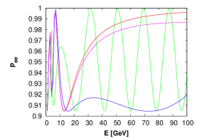
(a) Probability $P_{ee}$ as a function of energy at L=7000Km.

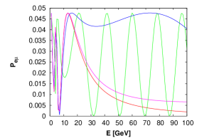
(b) Probability $P_{e\mu}$ as a function of energy at L=7000Km.

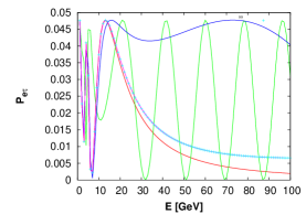
(c) Probability $P_{e\tau}$ as a function of energy at L=7000Km.

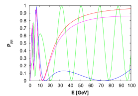
(d) Probability $P_{\mu\mu}$ as a function of energy at L=7000Km.

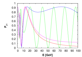
(e) Probability $P_{\mu\tau}$ as a function of energy at L=7000Km.

(f) Probability $P_{\tau\tau}$ as a function of energy at L=7000Km.

Figure 1: Velocity induced neutrino oscillation probabilities in vacuum (without MSW effect) and their comparisons when the effect of velocity induced oscillations are not present. The red lines in all the plots (a - f) are for the cases when velocity effect on the probabilities are not considered. The green, blue and pink lines represent the probabilities with velocity effects for $\Delta V=10^{-23},\,10^{-24},\,10^{-25}$ respectively in all the plots (a-f).

2.2 Velocity Induced Neutrino Oscillation in Matter: MSW Effect and Resonance

The passage of neutrinos through matter can considerably modify the neutrino oscillation probabilities. We study in this section how the velocity induced vacuum oscillation probabilities discussed earlier are modified when the matter effect (or MSW effect) is included. In the present context, this may be useful if one considers the case of baseline neutrinos from an accelerator or a neutrino factory propagating from their origin to a detector through the earth matter. In order to demonstrate the effect of different $\Delta V$ on the neutrino oscillation probabilities with matter effect, we have chosen a mean earth matter density of 4.15 gm/cc while the neutrinos traverse a representative baseline length of 7000 Km through the earth matter. The probabilities at different neutrino energies $E$ are calculated using Eqs. (73) - (79) and are plotted in Fig. 2a - 2f. As in Fig. 1, here too $P_{\alpha_{1}\alpha_{2}}$ represents the oscillation probability of a neutrino from flavour $\alpha_{1}$ to a flavour $\alpha_{2}$.

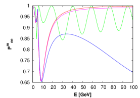
(a) Probability $P^{m}_{ee}$ as a function of energy at L=7000Km.

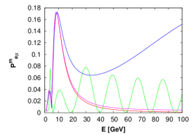
(b) Probability $P^{m}_{e\mu}$ as a function of energy at L=7000Km.

(c) Probability $P^{m}_{e\tau}$ as a function of energy at L=7000Km.

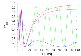
(d) Probability $P^{m}_{\mu\mu}$ as a function of energy at L=7000Km.

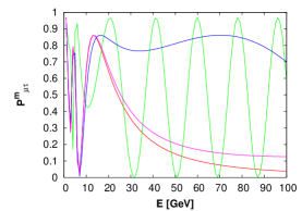
(e) Probability $P^{m}_{\mu\tau}$ as a function of energy at L=7000Km.

(f) Probability $P^{m}_{\tau\tau}$ as a function of energy at L=7000Km.

Figure 2: Velocity induced neutrino oscillation probabilities in matter and their comparisons when the effect of velocity induced oscillations are not present. The red lines in all the plots (a - f) are for the cases when velocity effect on the probabilities are not considered. The green, blue and pink lines represent the probabilities with velocity effects for $\Delta V=10^{-23},\,10^{-24},\,10^{-25}$ respectively in all the plots (a-f).

Fig. 2 demonstrates how the velocity induced oscillations affect the usual mass-flavour neutrino oscillation probabilities in presence of matter. For example, the electron neutrino survival probabilities $P^{m}_{ee}$ in Fig. 2a, although appears similar for the cases when $\Delta V=0$ and $\Delta V=10^{-25}$, the effect of $\Delta V$ shows up when $\Delta V=10^{-24}$ beyond $E\sim 15$ GeV. On the other hand, for $\Delta V=10^{-23}$, the variations of $P^{m}_{ee}$ with $E$ differ significantly not only from the case when velocity effect is absent ($\Delta V=0$) but also from the other two probabilities for two other $\Delta V$ values as well. This may also be noted that the shapes of $P^{m}_{ee}$ with matter effect (Fig. 2) differ from those without matter effect ($P_{ee}$ in Fig. 1) and these differences are more evident for the cases when $\Delta V=10^{-23}$ and $\Delta V=10^{-24}$. The variations of all the probabilities shown in Figs. 2a - 2f exhibit similar trends. Similar to vacuum oscillation scenario (without matter effect), here too the variations of probabilities exhibit multiple oscillatory behaviour for $\Delta V=10^{-23}$ although the natures of variations are notably different.

From the plots (a - f) in Fig. 2, this can be arguably stated that the effects of $\Delta V$ on the oscillation probabilities are indeed significant and this is most evident for $\Delta V=10^{-24}$ and $\Delta V=10^{-23}$ among the cases considered here. As mentioned earlier, for the latter case, the probabilities at different neutrino energies show a distinct multiple oscillatory nature in contrast to other probabilities. If many oscillations are accommodated in the oscillation length for the considered scenario then the probability would be averaged out. Comparison of Fig. 2 with Fig. 1 also clearly demonstrates that the matter effect modifies the vacuum probabilities (without matter effects). As an example, for $\Delta V=10^{-25}$ the value of $P^{m}_{e\tau}$, at a reference neutrino energy $E=10$ GeV, changes from 0.04 (Fig. 1) for no matter effect to 0.16 for the cases with matter effect (Fig. 2).

We also investigate the phenomenon of resonance which gives the maximal mixing between two neutrinos under the oscillation framework with matter effect. The possible occurence of resonance can be understood from Eq. (79) where the mixing angle $\Theta_{13,m}$ will be maximum when $R=\cos(2\Theta_{13})-2EV_{cc}/\Delta m_{32}^{{}^{\prime}2}=0$. Therefore, from Eq. (79), $\Theta_{13,m}=\frac{\pi}{4}$ at resonance. With $V_{cc}=\sqrt{2}G_{F}N_{e}$ (Eq. 69), the resonance condition is

$$\sqrt{2}G_{F}N_{e}=\frac{\Delta m_{32}^{{}^{\prime}2}}{2E}\cos(2\Theta_{13})\,.$$ (80)

The electron density $N_{e}$ in Eq. (80) can be obtained as $N_{e}=\rho N_{A}Y_{e}$, where $\rho$ is the density (the density of the earth in our case of long baseline neutrino), $N_{A}$ is the Avogadro number and $Y_{e}$ is the electron fraction. We calculate the variation of the quantity $R$ for three chosen values of matter densities namely $\rho=4.0,~{}4.15,~{}4.5$ gm/cc and for the three values of $\Delta V$ considered in this work. The results are plotted in Fig. 3(a - c). For all the calculations we restrict ourselves to the case of normal mass hierarchy for the neutrinos whereby $\Delta m_{32}^{{}^{\prime}2}>0$ ($\Delta m_{32}^{2}>0$ as well).

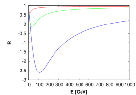
(a) $\cos(2\Theta_{13})-2EV_{cc}/\Delta m_{32}^{{}^{\prime}2}$ vs E for $\rho=4.00$ .

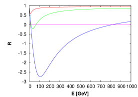
(b) $\cos(2\Theta_{13})-2EV_{cc}/\Delta m_{32}^{{}^{\prime}2}$ vs E for $\rho=4.15$ .

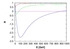
(c) $\cos(2\Theta_{13})-2EV_{cc}/\Delta m_{32}^{{}^{\prime}2}$ vs E for $\rho=4.50$ .

Figure 3: Effect of matter density $\rho$ on MSW resonance for different values of $\Delta V$

A discussion is in order. Using the expression for $\Delta m_{32}^{{}^{\prime}2}$ from Eq. (74), and substituing $\Delta V$ for $\Delta V_{32}$ as is done in this work, the expression for $R$ is given as

$$R = \cos(2\Theta_{13})-\frac{2\sqrt{2}G_{F}N_{e}E}{\Delta m^{2}_{32}+2\Delta VE^{2}}\,.$$ (81)

Fig. 3a - 3c shows that for any given non-zero value of $\Delta V$, the $R$ vs $E$ plots originate from a finite value ($\cos(2\Theta_{13})$) and then after reaching a minimum, asymptotically approach to the $\cos(2\Theta_{13})$ value for larger values of $E$. This behaviour can be easily understood from Eq. (81). The $E$ dependence of $R$ comes from the second term $\frac{2\sqrt{2}G_{F}N_{e}E}{\Delta m^{2}_{32}+2\Delta VE^{2}}(=X,~{}{\rm say})$ of the RHS of Eq. (81) through the combined effect of $E^{2}$ at the denominator (quadratic inverse) and $E$ (linear) at the numerator. Thus for low values of $E$, the quantity $R$ will decrease because of the negative term $X$ on the RHS of Eq. (81). But as $E$ increases, the $E^{2}$ in $X$ starts dominating over the linear $E$ dependence of $X$ and since $E^{2}$ is at the denominator, $X$ decreases faster than its increase with $E$, due to the linear $E$ dependence. This clearly explains the nature of $R$ vs $E$ plots in Fig. 3 discussed above. We mention in the passing that from Eq. (81), it is also evident that $R$ vs $E$ plot will be a straight line when $\Delta V=0$ (no velocity effects).

The resonance condition of Eq. (80) takes the form

$$\sqrt{2}G_{F}N_{e} = \left(\frac{\Delta m_{32}^{2}}{2E}+\Delta VE\right)\cos(2\Theta_{13})$$ (82)

$$= \left(\frac{\Delta m_{32}^{2}+2\Delta VE^{2}}{2E}\right)\cos(2\Theta_{13})\,.$$

Eq. (82) can be cast in the form

$$AE^{2}-BE+C = 0$$

$$A=2\Delta V\cos(2\Theta_{13}),~{}~{}B=2\sqrt{2}G_{F}N_{e}\,, C=\Delta m_{32}^{2}\cos(2\Theta_{13}).$$ (83)

The solutions of $E$ in Eq. (83) give the resonance energy $E_{R}$ for which the resonance condition (Eq. (80) or $R=0$) is satisfied.

The two solutions of $E$ in Eq. (83) are given by

$$E = \frac{B\pm\sqrt{B^{2}-4AC}}{2A}\,.$$ (84)

Eq. (84) has two real solutions for E when $B\geq\sqrt{B^{2}-4AC}$ and $B^{2}>4AC$. Thus we obtain two resonance energies $E_{R}$ when these conditions are satisfied. On the other hand, $E$ will have only one solution when the condition $B^{2}=4AC$ is satisfied. In that case the only solution will be $E=E_{R}=\frac{B}{2A}$ and imposing the condition $B^{2}=4AC$, one readily obtains, as the single soluion, $E_{R}=\sqrt{\frac{C}{A}}$. For computation of the quantities $A$, $B$ and $C$ (Eq. (83)) it is to be noted that $B$ is a constant for a chosen matter of known matter density $\rho$ through which the neutrinos traverse, $C$ is also a constant since the oscillation parameters $\Delta m_{32}^{2}$ and $\Theta_{13}$ are obtained from the neutrino experiments. For the computation of $A$, while the factor $\cos(2\Theta_{13})$ is fixed by the experimental value of $\Theta_{13}$, only the unknown velocity-induced oscillation parameter $\Delta V$ is varied (in the present work, as mentioned, three values are chosen for the same). This is also true for other conditions for two real solutions of the resonance energy (as also for obtaining no solutions). Therefore, the parameter $\Delta V$ dictates the various solutions of resonance energy for a given matter density.

One observes from the Fig. 3a - 3c that for $\Delta V=10^{-23}$ no resonance occurs. This means that for the chosen values of the matter densities, the resonance condition (Eq. 82) is not satisfied at all. The quantity $R$, for this $\Delta V$ value however passes through a minima and then approaches to its initial value of $\cos(\Theta_{13})$ as discussed above. For both the cases, when $\Delta V=10^{-24}$ and $\Delta V=10^{-25}$, the resonances occur twice at two different energy values. The difference between the two resonance energies should increase with the decrease of $\Delta V$ values and this also can be explained from the difference of two solutions in Eq. (84) which is $E_{r_{2}}-E_{r_{1}}=\sqrt{\frac{B^{2}}{A^{2}}-4\frac{C}{A}}$. Thus the effect of velocities-induced oscillations of neutrinos can also be manifested in the occruence of two resonances at two different energies. The results are summerised in Table 1.

Resonance energy $E_{r}$ for three different matter density $\rho$ and three diffrent values of $\Delta V$ $\rho~{}(N_{A}/cm^{3})$ $\Delta V$ Resonance energy $E_{r}$ in GeV 00 01E-23 0 No resonance 4.00 00 01E-24 018.70,061.50 01E-25 014.60,0787.70 01E-23 0 No resonance 4.15 00 01E-24 017.50,065.70 01E-25 014.10,0818.30 01E-23 0 No resonance 4.50 00 01E-24 015.40,074.90 01E-25 012.90,0889.60

However for antineutrinos, the interacting potenial is $-V_{cc}$. It is evident therefore that for antineutrinos, the resonance like phenomena will not occur unless $\Delta m_{32}^{2}$ is negative.

From the study of both Fig. 2 and Fig. 3, it can be said that among the three values of $\Delta V$ chosen for the present analysis, $\Delta V=10^{-24}$ is most effective. The choice $\Delta V=10^{-23}$ do not show any resonance phenomenon and the probability shows multiple oscillations. For the choice, $\Delta V=10^{-25}$, the resonance energies are wide apart (Fig. 3) and the probability almost coincide with that when velocity effects are absent.

3 Effect of Velocity Induced Oscillation on a Long Baseline Neutrino Experiment

We also investigate how the velocity induced oscillation affects the neutrino yield at a detector for long baseline neutrinos. In a long baseline neutrino experiment, the neutrinos are usually produced in a neutrino factory where the protons are bombarded on a target to form pions. The pions thus decay to yield muons. The muons are collected in a muon storage ring where they decay to produce muon and electron neutrinos following the processes $\mu^{-}\rightarrow e^{-}+\bar{\nu}_{e}+\nu_{\mu}$ and $\mu^{+}\rightarrow e^{+}+\nu_{e}+\bar{\nu}_{\mu}$. Neutrinos thus produced in a muon storage ring of a neutrino factory are then directed to a neutrino detector several kilometers (long baseline) away. These neutrinos have to traverse a distance through earth matter before reaching the detector.

The $\nu_{\mu}$($\bar{\nu}_{\mu}$) flux from such a neutrino factory is given by [17, 18]

$$\frac{d^{2}\Phi_{\nu_{\mu},\bar{\nu}_{\mu}}}{dydA}=\frac{4n_{\mu}}{\pi L^{2}m_{\mu}^{6}}\,\,E_{\mu}^{4}y^{2}\,(1-\beta)\,\,\left[3m_{\mu}^{2}-4E_{\mu}^{2}y\,(1-\beta)\right]$$ (85)

and the $\nu_{e}$($\bar{\nu}_{e}$) flux is given by

$$\frac{d^{2}\Phi_{\nu_{e},\bar{\nu}_{e}}}{dydA}=\frac{2n_{\mu}}{\pi L^{2}m_{\mu}^{6}}\,\,E_{\mu}^{4}y^{2}\,(1-\beta)\,\,\left[m_{\mu}^{2}-2E_{\mu}^{2}y\,(1-\beta)\right].$$ (86)

In Eqs. 85 - 86 the angle $\phi$ between the neutrino beam direction to the detector and the beam axis is taken to be zero and neutrinos are assumed to have no polarisation. In the above the quantity $E_{\mu}$ is the energy of the muon, $n_{\mu}$ denotes the number of muons injected in the storage ring, $L$ is the distance between the storage ring and detector, $m_{\mu}$ is the mass of the muon, $\beta$ is the boost factor and $y=\frac{E_{\nu}}{E_{\mu}}$, $E_{\nu}$ being the energy of the neutrino. Such long baseline neutrinos from a neutrino factory will suffer matter induced oscillation during its passage through earth matter to a far away detector. For the present calculation, we consider the far away detector to be an iron calorimeter (ICAL) made up of a stack of different layers of iron plates. A $\nu_{\mu}$ ($\bar{\nu}_{\mu}$), after reaching this ICAL detector will undergo charged current interaction with the iron of ICAL and produce track of $\mu^{-}$ ($\mu^{+}$) as they pass through diferent layers of ICAL detector. If the detector is magnetised, one can distinguish the tracks generated by $\mu^{+}$ or $\mu^{-}$. Thus from the nature of the track in ICAL, the detection of a $\nu_{\mu}$ or a $\bar{\nu}_{\mu}$ can be confirmed.

We consider such an ICAL detector at the proposed India-based Neutrino Observatory or INO [19], which is at a baseline length $\sim$ 7150 Km from a proposed neutrino factory at CERN. This length, being very near to the magic baseline length allows CP independent analysis of oscillation. ICAL at INO is proposed to be a 50 KTon detector consisting of a stack of 140 layers of iron plates of thickness 6 cm and interleaved with 2.5 cm gap. This is proposed to have a dimension of 48 m $\times$ 16 m $\times$ 12 m when complete[19]. The ICAL set up will be magnetised by a magnet of field strength $\sim 1.3$ Tesla.

A flux of $\nu_{\mu}$ from a $\mu^{-}$ storage ring (from the decay $\mu^{-}\rightarrow e^{-}+\bar{\nu}_{e}+\nu_{\mu}$) will suffer depletion on reaching the ICAL mentioned above due to oscillation of $\nu_{\mu}\rightarrow\nu_{\alpha_{x}}$, where $\alpha_{x}$ denotes any flavour other than $\mu$. This depleted $\nu_{\mu}$ flux will produce $\mu^{-}$ tracks at the magnetised ICAL detector, in this disappearance channel. These $\mu^{-}$ are referred to as right sign muons. If on the other hand ICAL registers $\mu^{+}$ tracks from such a beam then this would imply the appearance of $\bar{\nu}_{\mu}$ at ICAL which can be obtained in the beam (of $\nu_{\mu}$ and $\bar{\nu}_{e}$) due to the oscillation process $\bar{\nu}_{e}\rightarrow\bar{\nu}_{\mu}$. This is the appearance channel. Such $\mu^{+}$ are wrong sign muons.

In the present work, for the purpose of demonstration we have taken the injected muon energy at storage ring to be 50 GeV with the estimated baseline length of CERN-ICAL distance. The disttance between CERN to the proposed site for the ICAL is calulated to be $L=7154.57$ Km. The average earth matter density ($\rho$) for this baseline is taken to be 4.15 gm/cc. The $\nu_{\mu}$ and $\bar{\nu}_{e}$ flux at the ICAL detector for such neutrino beam (assumed to have originated from CERN and contains in the beam ${\nu}_{\mu}$ and $\bar{\nu}_{e}$) are calculated using Eqs. 85 - 86 for 5 years of run and are plotted in plots (a) and (b) respectively of Fig. 4.

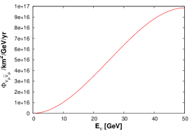
(a) Variation of $\Phi_{\nu_{\mu},\bar{\nu}_{\mu}}$ with $E_{\nu}$ at CERN-INO for injected muon energy fixed at 50 GeV

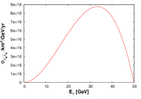
(b) Variation of $\Phi_{\nu_{e},\bar{\nu}_{e}}$ with $E_{\nu}$ at CERN-INO for injected muon energy fixed at 50 GeV

Figure 4: $\nu_{\mu}$($\bar{\nu}_{\mu}$) flux (plot a) and $\nu_{e}$($\bar{\nu}_{e}$) flux (plot b) for different neutrino energies ($E_{\nu}$) in case of a 50 GeV $\mu^{-}$ ($E_{\mu}=50$ GeV) decaying in a storage ring for a period of 5 years. The baseline length $L=7154.57$ Km

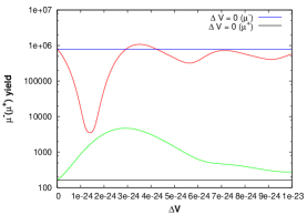
Figure 5: Dependence of $\mu^{\pm}$ yield in the prescence of velocity dependant oscillation of neutrinos

From the knowledge of the flux $\phi_{\nu_{\mu}}$ and $\phi_{\nu_{e}}$ (Fig. 4), the oscillation probabilities $P_{\nu_{\mu}\rightarrow\nu_{x}}$ (for disappearance channel) and $P_{{\bar{\nu}_{e}}\rightarrow\bar{\nu}_{\mu}}$ (for appearance channel) and the cross-section for the charged interactions of $\nu_{\mu}(\bar{\nu}_{\mu})$ with iron that will produce $\mu^{-}(\mu^{+})$ at ICAL, the yields of $\mu^{-}$ and $\mu^{+}$ can be computed. In this work we compute the $\mu^{-}$ (right sign) yields and $\mu^{+}$ (wrong sign) yields at the ICAL detector considered here with oscillation probabilities that include velocity effects as well as matter effects for a baseline length of 7154.57 Km. In Fig. 5 we demonstrate the variation of these $\mu$-yields as a function of velocity difference ($\Delta V$) between two neutrino species while $\Delta V$ is varied from zero (no velocity oscillation) to $\Delta V=10^{-23}$. Red (green) line in Fig. 5 corresponds to the yield of right sign (wrong sign) $\mu$ for a run period of 5 years. The blue and black lines in Fig. 5 represent the right and wrong sign muon yields respectively when $\Delta V=0$. It is evident from Fig. 5 that velocity induced oscillation significantly affects the yields of $\mu$ when compared with the case of normal mass-flavour oscillation ($\Delta V=0$). It can also be observed from the plots in Fig. 5 that right sign $\mu$ yield decreaes rapidly for $\Delta V\sim 1-2\times 10^{-24}$ and then it saturates to a value appproximaltely to the yield when $\Delta V=0$ for the remaining range ($\Delta V=10^{-23}$). Conversely yield of the wrong sign $\mu$ increases nearly an order of magnitude for $\Delta V\sim 1-5\times 10^{-24}$. For higher values of $\Delta V$, yields of wrong sign $\mu$ also tend to saturate to the yield corresponding to normal mass flavour oscillation. One can also conclude from Fig. 5 that considerable changes in both right and wrong sign $\mu$ yields are observed near $\Delta V\sim 10^{-24}$. In Table 2 we tabulate the estimated yields for a run period of 5 years. Results are shown for the three values of velocity difference, namely, $\Delta V$ ($\Delta V=10^{-23},~{}10^{-24},~{}10^{-25}$) as adopted in Section 2. The results with $\Delta V=0$ (no velocity effect) are also given in Table 2 for comparison.

The right sign $\mu$ yield and wrong sign $\mu$ yield at the ICAL detector with baseline length of 7154.57 Km in case of different values of $\Delta V$ with injected muon energy fixed at 50 GeV.                           CERN-ICAL                Baseline length ($L$) 7154.57 Km $\Delta V$ Right sign $\mu$ Wrong sign $\mu$           0.0 794147 161           1E-23 575795 278           1E-24 17132 871           1E-25 663325 183

It is evident from the comparison of the calculated yields of right sign and wrong sign muons in Table 3 that the velocity induced oscillation indeed affects the yields significantly when compared with the normal mass-flavour oscillation ($\Delta V=0$). Among the chosen three values of $\Delta V$, while the effect of $\Delta V$ is negligible for $\Delta V=10^{-25}$, this is most pronounced for the case when $\Delta V=10^{-24}$. For the latter case, the calculated right sign muon is an order of magnitude less than for the case $\Delta V=0$ and there is almost an order of magnitude gain ($\sim 10^{2}$ for $\Delta V=0$ to $\sim 10^{3}$ with $\Delta V=10^{-24}$) for wrong sign muon when $\Delta V=10^{-24}$ over the case with no velocity effect. More statistics for the wrong sign muons are in fact helpful for the study of crucial $\nu_{e}\rightarrow\nu_{\mu}$ oscillations.

4 Summary and Conclusion

In the present work, the effect of velocity induced neutrino oscillation is explored in the 3-generation framework of neutrinos. This is based on the consideration that the three different neutrinos can have three different maximum attainable velocities and their flavour eigenstates are not the same as their velocity eigenstates and mass eigenstates. The oscillation phenomena in this scenario are studied with modifying the Hamiltonian in the mass basis by adding the Hamiltonian in the velocity basis and then the evolution equations for the neutrino flavours are written down in terms of this modified Hamiltonian. Thus we have the formalism for neutrino flavour oscillations induced by both mass and velocity. Unlike for the case of purely mass-induced flavour oscillation, where the phase difference of two neutrinos (that causes the oscillation) $\sim\frac{1}{E}$, for purely velocity-induced flavour oscillation the phase difference $\sim E$. Thus we study in this work, the combined effect of both of them on neutrino flavour oscillations in the realistic case of three generations.

For demonstrative purposes, we consider the case of baseline neutrinos with a representative baseline length of 7000 Km. The oscillation probabilities are computed for this example first by considering no matter effect (vacuum oscillations) and then by incorporating the matter effect or MSW effect in the present formalism. Three values of $\Delta V$ ($\Delta V=10^{-23},10^{-24},10^{-25}$) are chosen for the calculation and the results are compared with the case when no velocity effect is present ($\Delta V=0$). We found that near the vicinity of $\Delta V\sim 10^{-24}$ velocity induced oscillation effect provides significant change in oscillation when comapred with the normal mass flavour oscillation scenario for the case of long baseline neutrino oscillation with baseline length $L\sim 7000$ Km. Also it appears that the choice of $\Delta V$ values, further order of magnitude lower than this value (such as $\Delta V=10^{-25}$), in fact produces almost or no velocity-induced effects on oscillation probabilities. On the other hand, when $\Delta V$ is chosen to be order of magnitude higher than the value of $10^{-24}$ (such as for $\Delta V=10^{-23}$), the probabilities show rapid oscillatory nature. It is also seen that while the MSW resonance condition is saisfied for two values of resonance energies for both the choices of $\Delta V=10^{-24}$ and $\Delta V=10^{-25}$, the choice $\Delta V=10^{-23}$ yields no resonance since such a choice does not satisfy the resonance condition. The two values of resonance energies are however expected as here the effects of both $\sim E$ and $\sim\frac{1}{E}$ dependences reduce the resonance condition to an equation quadratic in $E$.

Hence the Hamiltonian of time evolution of neutrinos will be changed in presence of velocity mixing oscillation. We investigate the possible effects of the inclusion of the velocity dependent states that modify the normal mass oscillation scenario. In the present formalism, the unitary matrix connecting flavour and mass basis also connects flavour basis to velocity basis. This gives modified oscillation probability equations and we plot the different probabilities as a function of energy with and without presence of matter. We study how the presence of velocity dependent states can change the different oscillation probabilities $P_{\alpha_{1}\alpha_{2}}$ and its effects on resonance phenomena. We find that in some cases velocity induced oscillations differ significantly from normal (flavour - mass) oscillation of neutrinos.

We then apply our results for the case of a possible long baseline neutrino experiment. For this purpose we have considered a magnetised iron calorimeter detector (ICAL) at the proposed India-based Neutrino Observatory (INO) [19] as the end detector that would detect the muon neutrinos in a neutrino beam of $\nu_{\mu}$ and $\bar{\nu}_{e}$ considered to have originated from a possible neutrino factory at CERN having baseline length $\sim 7154$ Km. The muon neutrinos would produce muons following their charged current interactions with iron of ICAL and identifying the polarities of such muon signals, $\mu^{-}$ or $\mu^{+}$ at ICAL, since the latter is magnetised, the nature of the detected neutrinos (whether it is $\nu_{\mu}$ or $\bar{\nu}_{\mu}$) can be concluded. While the $\mu^{-}$ events in the present example are termed as the right sign muons indicating the detection of $\nu_{\mu}$ the flux of which would suffer depletion in the beam due to oscillation in disappearance channel, detecting of the wrong sign muons or $\mu^{+}$ definitely indicate the oscillation $\bar{\nu}_{e}\rightarrow\bar{\nu}_{\mu}$ in the appearance channel. In order to show how velocity induced oscillation affects the $\mu^{\pm}$ yield, we plot $\mu^{\pm}$ yield as a function of $\Delta V$ in the present formalism. Here too we find that $\mu^{\pm}$ yield changes drastically for some choice of $\Delta V$ $(\sim 10^{-24}$). We also find that the estimated number of wrong sign muons is considerably large in the range of $\Delta V\sim 1-5\times 10^{-24}$ which is helpful for effective statistical analysis of this important disappearnce channel. Finally it could be concluded that, neutrino oscillation experiments in near future capable of probing the velocity differences between nuetrino species and also the respective $\mu$ yield are expected to provide valuable information to enlighten the velocity induced neutrino oscillation or rule out the possibility of such velocity induced neutrino oscillation.

References

- [1] H. Minakata and A. Yu Smirnov, Phys. Rev. D 54, 3698 (1996).
- [2] R. B. Mann and U. Sarkar, Phys. Rev. Lett. 76, 865 (1996).
- [3] D. Majumdar, A. Raychaudhuri and A. Sil, Phys. Rev. D 63, 073014 (2001).
- [4] S. Coleman and S. L. Glashow, Phys. Lett. B 405, 249 (1997).
- [5] G.L. Fogli, E. Lisi, A. Marone and G. Scioscia, Phys. Rev. D 60, 053006 (1999) and references therein.
- [6] G. Battistoni et al, Phys. Lett. B 615, 14 (2005).
- [7] S. Ahlen, et al., Nucl. Instrum. Meth. A 324, 337 (1993).
- [8] M. Ambrosio, et al., Nucl. Instrum. Meth. A 486, 663 (2002).
- [9] M.C. Gonzalez-Garcia and M. Maltoni, Phys. Rep. 460, 1 (2008) and references therein.
- [10] B. Pontecorvo, Sov. Phys. JETP 6, 429 (1958).
- [11] B. Pontecorvo, Sov. Phys. JETP 7, 172 (1958).
- [12] C. Giunti, C.W. Kim, M. Monteno, Nucl. Phys. B 521, 3 (1998).
- [13] E. Kh. Akhmedov, arXiv:hep-ph/0001264.
- [14] M.C. Gonalez-Garcia and Y. Nir, Rev. of Mod. Phys. 75, 345 (2003).
- [15] G. L. Fogli et. al., Phys. Rev. D 86, 013012 (2012).
- [16] T. Thakore et. al. JHEP 05, 058 (2013).
- [17] S. Geer, Phys. Rev. D 57, 6989 (1998).
- [18] A. Donini, D. Meloni and P. Migliozzi, Nucl. Phys. B 646, 321 (2002).
- [19] V. Arunagam et al, INO Interim Project Report, Vol. 1, (INO collaboration), (2005).