Spatio-Temporal Analysis of Epidemic Phenomena Using the R Package surveillance

Sebastian Meyer, Leonhard Held, Michael Höhle Spatio-Temporal Analysis of Epidemic Phenomena Using the R Package surveillance surveillance: Spatio-Temporal Analysis of Epidemic Phenomena The availability of geocoded health data and the inherent temporal structure of communicable diseases have led to an increased interest in statistical models and software for spatio-temporal data with epidemic features. The open source R package surveillance can handle various levels of aggregation at which infective events have been recorded: individual-level time-stamped geo-referenced data (case reports) in either continuous space or discrete space, as well as counts aggregated by period and region. For each of these data types, the surveillance package implements tools for visualization, likelihoood inference and simulation from recently developed statistical regression frameworks capturing endemic and epidemic dynamics. Altogether, this paper is a guide to the spatio-temporal modeling of epidemic phenomena, exemplified by analyses of public health surveillance data on measles and invasive meningococcal disease. spatio-temporal surveillance data, endemic-epidemic modeling, infectious disease epidemiology, self-exciting point process, multivariate time series of counts, branching process with immigration Sebastian Meyer
Epidemiology, Biostatistics and Prevention Institute
University of Zurich
Hirschengraben 84
CH-8001 Zurich, Switzerland
E-mail:
URL: http://www.ebpi.uzh.ch/en/aboutus/departments/biostatistics.html Leonhard Held
Epidemiology, Biostatistics and Prevention Institute
University of Zurich
E-mail: Michael Höhle
Department of Mathematics
Stockholm University
E-mail:
URL: http://www.math.su.se/~hoehle

1 Introduction

Epidemic data are realizations of spatio-temporal processes with autoregressive or “self-exciting” behavior. Examples of epidemic phenomena beyond infectious diseases include earth quakes (Ogata, 1999), crimes (Johnson, 2010; Mohler et al., 2011), invasive species (Balderama et al., 2012), and forest fires (Vrbik et al., 2012). Epidemic data are special with regard to at least three aspects, which hinder the application of classical statistical approaches: the data are rarely a result of planned experiments, the observations (cases, events) are not independent, and often the process is only partially observable.

Since 2005, the open source R (R Core Team, 2015) package surveillance provides a growing computational framework for methodological developments and practical tools for the monitoring and modeling of epidemic phenomena – traditionally in the context of infectious diseases. Monitoring is concerned with prospective aberration detection for which several algorithms have been implemented as described by Höhle (2007) and recently updated and reviewed by Salmon et al. (2015). The other major purpose of the surveillance package and the focus of this paper is the regression-oriented modeling of spatio-temporal epidemic data. This enables the user to a) assess the role of environmental factors, socio-demographic characteristics, or control measures in shaping endemic and epidemic dynamics, b) analyze the spatio-temporal interaction of events, and c) simulate the epidemic spread from estimated models.

The implemented statistical modeling frameworks have already been successfully applied to a broad range of surveillance data, e.g., human influenza (Paul et al., 2008; Paul and Held, 2011; Geilhufe et al., 2014), meningococcal disease (Paul et al., 2008; Paul and Held, 2011; Meyer et al., 2012), measles (Herzog et al., 2011), psychiatric hospital admissions (Meyer et al., 2015), rabies in foxes (Höhle et al., 2009), coxiellosis in cows (Schrödle et al., 2012), and the classical swine fever virus (Höhle, 2009). Although these applications all originate from public or animal health surveillance, we stress that our methods also apply to the other epidemic phenomena described above.

To the best of our knowledge, no other software can estimate regression models for spatio-temporal epidemic data. There are, however, some related R packages that we like to mention here, since they also deal with epidemic phenomena. For instance, the R-epi project lists the package EpiEstim (Cori et al., 2013), which can estimate the average number of secondary cases caused by an infected individual, the so-called reproduction number, from a time series of disease incidence. Similar functionality is provided by the package R0 (Obadia et al., 2012). Other packages are designed to estimate transmission characteristics from phylogenetic trees (TreePar, Stadler and Bonhoeffer, 2013), or to reconstruct transmission trees from sequence data (outbreaker, Jombart et al., 2014). The package amei (Merl et al., 2010) is targeted towards finding optimal intervention strategies, e.g., the proportion of the population to be vaccinated to prevent further disease spread, using purely temporal epidemic models. The recently published package tscount (Liboschik et al., 2015) is dedicated to the analysis of count time series with serial correlation such as the number of stock market transitions per minute or the weekly number of reported infections of a particular disease. The tscount package can fit a univariate version of the areal count time-series model presented in Section 5. For a purely spatial analysis of disease occurrence, see, e.g., the recent paper by Brown (2015) introducing the package diseasemapping. One of the few packages fitting spatio-temporal epidemic models is etasFLP (Adelfio and Chiodi, 2015). The Epidemic-Type Aftershock-Sequences (ETAS) model for earthquakes (Ogata, 1999) is closely related to the endemic-epidemic point process model described in Section 3, but incorporates seismological laws rather than covariates. The long-standing package splancs (Rowlingson and Diggle, 2015) offers diagnostic tools to investigate space-time clustering in a point pattern, i.e., to check if the process at hand shows self-exciting epidemic behavior. Statistical tests for space-time interaction are discussed in Meyer et al. (2015), who propose a test based on the regression framework of Section 3. An important recent development for spatio-temporal tasks in R are the basic data classes and utility functions provided by the dedicated package spacetime (Pebesma, 2012), which builds upon the quasi standards sp (Bivand et al., 2013) for spatial data and xts (Ryan and Ulrich, 2014) for time-indexed data, respectively. For a more general overview of R packages for spatio-temporal data, see the CRAN Task View “Handling and Analyzing Spatio-Temporal Data” (Pebesma, 2015). A non-R option is the Spatiotemporal Epidemiological Modeler (STEM) tool. It has a graphical user interface and can simulate the evolution of disease incidence in a population. The ability to estimate model parameters from surveillance data, however, is limited to simple non-spatial models. WinBUGS has been used for Bayesian inference of specialized spatio-temporal epidemic models (Malesios et al., 2014).

The remainder of this paper is organized as follows: Section 2 gives a brief overview of the three statistical models for spatio-temporal epidemic data implemented in surveillance. Each of the subsequent model-specific Sections 3 to 5 first describes the associated methodology and then illustrates the model implementation – including data handling, visualization, inference, and simulation – by applications to infectious disease surveillance data. Section 6 concludes the paper.

2 Spatio-temporal endemic-epidemic modeling

Epidemic models traditionally describe the spread of a communicable disease in a population. Often, a compartmental view of the population is taken, placing individuals into one of the three states (S)usceptible, (I)nfectious, or (R)emoved. Modeling the transitions between these states in a closed population using deterministic differential equations dates back to the work of Kermack and McKendrick (1927). Considering a stochastic version of the simplest homogeneous SIR model in a closed population of size $N$, the hazard rate for a susceptible individual $i\in S(t)$ to become infectious at time $t$ – the so-called force of infection – is

$$\lambda_{i}(t)=\sum_{j\in I(t)}\beta\>.$$ (1)

Here, $S(t),I(t)\subseteq\{1,\dotsc,N\}$ denote the index sets of currently susceptible and infectious individuals, respectively, and the parameter $\beta>0$ is called the transmission rate. The stochastic SIR model is complemented by a distributional assumption about how long individuals are infective, where typical choices are the exponential or the gamma distribution. The set of recovered individuals at time $t$ is found as $R(t)=\{1,\dotsc,N\}\setminus(S(t)\cup I(t))$. The above homogeneous SIR model has since been extended in a multitude of ways, e.g., by additional states (addressing population heterogeneities arising from age groups, spatial location or vaccination) or population demographics. Overviews of SIR modeling approaches can be found in Anderson and May (1991), Daley and Gani (1999), and Keeling and Rohani (2008). The estimation of SIR model parameters from actual observed data is, however, often only treated marginally in such descriptions. In contrast, a number of more statistically flavored epidemic models have emerged recently. This includes, e.g., the TSIR model (Finkenstädt and Grenfell, 2000), two-component time-series models (Held et al., 2005, 2006), and point process models (Lawson and Leimich, 2000; Diggle, 2006). An overview of temporal and spatio-temporal epidemic models and their relation to the underlying metapopulation SIR models can be found in Höhle (2016).

At the heart of any statistical analysis is the subject-matter scientific problem, which a data-driven analysis seeks to address. Due to the generality and complexity of such problems we adopt here a technocratic view and let the available data guide what a “useful” epidemic model is. The surveillance package offers regression-oriented modeling frameworks for three different types of spatio-temporal data distinguished by the spatial and temporal resolution (Table 1). First, if an entire region is continuously monitored for infective events, which are time-stamped, geo-referenced, and potentially enriched with further event-specific data, then a (marked) spatio-temporal point pattern arises. Such continuous space-time epidemic data can be viewed as a realization of a self-exciting spatio-temporal point process (Section 3). The second data type we consider comprises the event history of a discrete set of units followed over time – e.g., farms during livestock epidemics – while registering when they become susceptible, infected, and potentially removed (neither at risk nor infectious). These data fit into the framework of a spatial SIR model represented as a multivariate temporal point process (Section 4). Our third data type is often encountered as a result of privacy protection or reporting regimes, and is an aggregated version of the individual event data mentioned first: event counts by region and period. Such areal count time series can be fitted with the multivariate negative binomial time-series model presented in Section 5.

The three aforementioned model classes are all inspired by the Poisson branching process with immigration approach proposed by Held et al. (2005). Its main characteristic is the additive decomposition of disease risk into endemic and epidemic features, similar to the background and triggered components in the ETAS model for earthquake occurrence. The endemic component describes the risk of new events by external factors independent of the history of the epidemic process. In the context of infectious diseases, such factors may include seasonality, population density, socio-demographic variables, and vaccination coverage – all potentially varying in time and/or space. Explicit dependence between events is then introduced through an epidemic component driven by the observed past.

Each of the following three model-specific sections starts with a brief theoretical introduction to the respective spatio-temporal endemic-epidemic model, before we describe the implementation using the example data mentioned in Table 1.

	twinstim (Section 3)	twinSIR (Section 4)	hhh4 (Section 5)
Data class	epidataCS	epidata	sts
Resolution	individual events in	individual SI[R][S] event	event counts aggregated
	continuous space-time	history of a fixed population	by region and time period
Example	cases of meningococcal	measles outbreak among	weekly counts of measles by
	disease, Germany, 2002–8	children in Hagelloch, 1861	district, Weser-Ems, 2001–2
Model	(marked) spatio-temporal	multivariate temporal	multivariate time series
	point process	point process	(Poisson or NegBin)
Reference	Meyer et al. (2012)	Höhle (2009)	Held and Paul (2012)

Table 1: Spatio-temporal endemic-epidemic models and corresponding data classes implemented in the R package surveillance.

3 Spatio-temporal point pattern of infective events

The endemic-epidemic spatio-temporal point process model “twinstim” is designed for point-referenced, individual-level surveillance data. As an illustrative example, we use case reports of invasive meningococcal disease (IMD) caused by the two most common bacterial finetypes of meningococci in Germany, 2002–2008, as previously analyzed by Meyer et al. (2012) and Meyer and Held (2014a). We start by describing the general model class in Section 3.1. Section 3.2 introduces the example data and the associated class epidataCS, Section 3.3 presents the core functionality of fitting and analyzing such data using twinstim, and Section 3.4 shows how to simulate realizations from a fitted model.

3.1 Model class: twinstim

Infective events occur at specific points in continuous space and time, which gives rise to a spatio-temporal point pattern $\{(\bm{s}_{i},t_{i}):i=1,\dotsc,n\}$ from a region $\bm{W}$ observed during a period $(0,T]$. The locations $\bm{s}_{i}$ and time points $t_{i}$ of the $n$ events can be regarded as a realization of a self-exciting spatio-temporal point process, which can be characterized by its conditional intensity function (CIF, also termed intensity process) $\lambda(\bm{s},t)$. It represents the instantaneous event rate at location $\bm{s}$ at time point $t$ given all past events, and is often more verbosely denoted by $\lambda^{*}$ or by explicit conditioning on the “history” $\mathcal{H}_{t}$ of the process. Daley and Vere-Jones (2003, Chapter 7) provide a rigorous mathematical definition of this concept, which is key to likelihood analysis and simulation of “evolutionary” point processes.

Meyer et al. (2012) formulated the model class “twinstim” – a two-component spatio-temporal intensity model – by a superposition of an endemic and an epidemic component:

$$\lambda(\bm{s},t)=\nu_{[\bm{s}][t]}+\sum_{j\in I(\bm{s},t)}\eta_{j}\,f(\lVert\bm{s}-\bm{s}_{j}\rVert)\,g(t-t_{j})\>.$$ (2)

This model constitutes a branching process with immigration, where part of the event rate is due to the first, endemic component, which reflects sporadic events caused by unobserved sources of infection. This background rate of new events is modelled by a piecewise constant log-linear predictor $\nu_{[\bm{s}][t]}$ incorporating regional and/or time-varying characteristics. Here, the space-time index $[\bm{s}][t]$ refers to the region covering $\bm{s}$ during the period containing $t$ and thus spans a whole spatio-temporal grid on which the involved covariates are measured, e.g., district $\times$ month. We will later see that the endemic component therefore simply equals an inhomogeneous Poisson process for the event counts by cell of that grid.

The second, observation-driven epidemic component adds “infection pressure” from the set

$$I(\bm{s},t)=\big{\{}j:t_{j}<t\>\wedge\>t-t_{j}\leq\tau_{j}\>\wedge\>\lVert\bm{s}-\bm{s}_{j}\rVert\leq\delta_{j}\big{\}}$$

of past events and hence makes the process “self-exciting”. During its infectious period of length $\tau_{j}$ and within its spatial interaction radius $\delta_{j}$, the model assumes each event $j$ to trigger further events, which are called offspring, secondary cases, or aftershocks, depending on the application. The triggering rate (or force of infection) is proportional to a log-linear predictor $\eta_{j}$ associated with event-specific characteristics (“marks”) $\bm{m}_{j}$, which are usually attached to the point pattern of events. The decay of infection pressure with increasing spatial and temporal distance from the infective event is modelled by parametric interaction functions $f$ and $g$, respectively (Lawson and Leimich, 2000, Section 4). A simple assumption for the time course of infectivity is $g(t)=1$. Alternatives include exponential decay, a step function, or empirically derived functions such as Omori’s law for aftershock intervals (Utsu et al., 1995). With regard to spatial interaction, the statistician’s standard choice is a Gaussian kernel $f(x)=\exp\left\{-x^{2}/(2\sigma^{2})\right\}$. However, in modeling the spread of human infectious diseases on larger scales, a heavy-tailed power-law kernel $f(x)=(x+\sigma)^{-d}$ was found to perform better (Meyer and Held, 2014a). The (possibly infinite) upper bounds $\tau_{j}$ and $\delta_{j}$ provide a way of modeling event-specific interaction ranges. However, since these need to be pre-specified, a common assumption is $\tau_{j}\equiv\tau$ and $\delta_{j}\equiv\delta$, where the infectious period $\tau$ and the spatial interaction radius $\delta$ are determined by subject-matter considerations.

3.1.1 Model-based effective reproduction numbers

Similar to the simple SIR model (see, e.g., Keeling and Rohani, 2008, Section 2.1), the above point process model (2) features a reproduction number derived from its branching process interpretation. As soon as an event occurs (individual becomes infected), it triggers offspring (secondary cases) around its origin $(\bm{s_{j}},t_{j})$ according to an inhomogeneous Poisson process with rate $\eta_{j}\,f(\lVert\bm{s}-\bm{s_{j}}\rVert)\,g(t-t_{j})$. Since this triggering process is independent of the event’s parentage and of other events, the expected number $\mu_{j}$ of events triggered by event $j$ can be obtained by integrating the triggering rate over the observed interaction domain:

$$\mu_{j}=\eta_{j}\cdot\left[\int_{0}^{\min(T-t_{j},\tau_{j})}g(t)\,dt\right]\cdot\left[\int_{\bm{R}_{j}}f(\lVert\bm{s}\rVert)\,d\bm{s}\right]\>,$$ (3)

where

$$\bm{R}_{j}=(b(\bm{s}_{j},\delta_{j})\cap\bm{W})-\bm{s}_{j}$$ (4)

is event $j$’s influence region centered at $\bm{s}_{j}$, and $b(\bm{s}_{j},\delta_{j})$ denotes the disc centered at $\bm{s}_{j}$ with radius $\delta_{j}$. Note that the above model-based reproduction number $\mu_{j}$ is event-specific since it depends on event marks through $\eta_{j}$, on the ranges of interaction $\delta_{j}$ and $\tau_{j}$, as well as on the event location $\bm{s}_{j}$ and time point $t_{j}$.

Equation 3 can also be motivated by looking at a spatio-temporal version of the simple SIR model (1) wrapped into the twinstim class (2). This means: no endemic component, homogeneous force of infection ($\eta_{j}\equiv\beta$), homogeneous mixing in space ($f(x)=1$, $\delta_{j}\equiv\infty$), and exponential decay of infectivity ($g(t)=e^{-\alpha t}$, $\tau_{j}\equiv\infty$). Then, for $T\rightarrow\infty$,

$$\mu=\beta\cdot\left[\int_{0}^{\infty}e^{-\alpha t}\,dt\right]\cdot\left[\int_{\bm{W}-\bm{s_{j}}}1\,d\bm{s}\right]=\beta\cdot\lvert\bm{W}\rvert/\alpha\>,$$

which corresponds to the basic reproduction number known from the simple SIR model by interpreting $\lvert\bm{W}\rvert$ as the population size, $\beta$ as the transmission rate and $\alpha$ as the removal rate. Like in classic epidemic models, the process is sub-critical if $\mu<1$ holds, which means that its eventual extinction is almost sure.

However, it is crucial to understand that in a full model with an endemic component, new infections may always occur via “immigration”. Hence, reproduction numbers in twinstim are adjusted for infections occurring independently of previous infections. This also means that a misspecified endemic component may distort model-based reproduction numbers (Meyer et al., 2015). Furthermore, under-reporting and implemented control measures imply that the estimates are to be thought of as effective reproduction numbers.

3.1.2 Likelihood inference

The log-likelihood of the point process model (2) is a function of all parameters in the log-linear predictors $\nu_{[\bm{s}][t]}$ and $\eta_{j}$ and in the interaction functions $f$ and $g$. It has the form

$$\left[\sum_{i=1}^{n}\log\lambda(\bm{s}_{i},t_{i})\right]-\int_{0}^{T}\int_{\bm{W}}\lambda(\bm{s},t)\,\mathrm{d}\bm{s}\,\mathrm{d}t\>.$$ (5)

To estimate the model parameters, we maximize the above log-likelihood numerically using the quasi-Newton algorithm available through the R function nlminb. We thereby make use of the analytical score function and an approximation of the expected Fisher information worked out by Meyer et al. (2012, Web Appendices A and B).

The space-time integral in the log-likelihood poses no difficulties for the endemic component of $\lambda(\bm{s},t)$ since it is piecewise constant. However, integration of the epidemic component has a clear computational bottleneck: two-dimensional integrals $\int_{\bm{R}_{i}}f(\lVert\bm{s}\rVert)\,\mathrm{d}\bm{s}$ over the influence regions $\bm{R}_{i}$ of Equation 4, which are computationally represented by polygons (as is $\bm{W}$). Similar integrals appear in the score function, where $f(\lVert\bm{s}\rVert)$ is replaced by partial derivatives with respect to kernel parameters, e.g., $\partial f(\lVert\bm{s}\rVert)/\partial\log\sigma$ for the Gaussian kernel with standard deviation estimated on the log-scale. Calculation of these integrals is trivial for (piecewise) constant $f$, but otherwise requires numerical integration. For this purpose, the R package polyCub (Meyer, 2015) offers cubature methods for polygonal domains as described in Meyer and Held (2014b, Section 2). For Gaussian $f$, we apply the two-dimensional midpoint rule with a $\sigma$-adaptive bandwidth, combined with an analytical formula via the $\chi^{2}$ distribution if the $6\sigma$-circle around $\bm{s}_{i}$ is contained in $\bm{R}_{i}$ (Meyer et al., 2012). The integrals in the score function are approximated by product Gauss cubature (Sommariva and Vianello, 2007). For the recently implemented power-law kernels (Meyer and Held, 2014a), we apply a particularly appealing method which takes analytical advantage of the assumed isotropy of spatial interaction in such a way that numerical integration remains in only one dimension (Meyer and Held, 2014b, Section 2.4). As a general means to reduce the computational burden during numerical log-likelihood maximization, we memoise (Wickham, 2014) the cubature function, which avoids redundant re-evaluations of the integral with identical parameters of $f$.

3.1.3 Special case: Endemic-only twinstim

As mentioned above, a twinstim model without an epidemic component can actually be represented as a Poisson regression model for aggregated counts. This provides a nice link to ecological regression approaches in general (Waller and Gotway, 2004) and to the count data model hhh4 illustrated in Section 5. To see this, recall that the endemic component $\nu_{[\bm{s}][t]}$ of a twinstim (2) is piecewise constant on the spatio-temporal grid with cells $([\bm{s}],[t])$. Hence the log-likelihood (5) of an endemic-only twinstim simplifies to a sum over all these cells,

$$\sum_{[\bm{s}],[t]}\left\{Y_{[\bm{s}][t]}\log\nu_{[\bm{s}][t]}-\lvert[\bm{s}]\rvert\,\lvert[t]\rvert\,\nu_{[\bm{s}][t]}\right\}\>,$$

where $Y_{[\bm{s}][t]}$ is the aggregated number of events observed in cell $([\bm{s}],[t])$, and $\lvert[\bm{s}]\rvert$ and $\lvert[t]\rvert$ denote cell area and length, respectively. Except for an additive constant, the above log-likelihood is equivalently obtained from the Poisson model $Y_{[\bm{s}][t]}\sim\operatorname{Po}(\lvert[\bm{s}]\rvert\,\lvert[t]\rvert\,\nu_{[\bm{s}][t]})$. This relation offers a means of code validation using the established glm function to fit an endemic-only twinstim model, see the examples in help("glm_epidataCS").

3.1.4 Extension: twinstim with event types

To model the example data on invasive meningococcal disease in the remainder of this section, we actually need to use an extended version $\lambda(\bm{s},t,k)$ of Equation 2, which accounts for different event types $k$ with own transmission dynamics. This introduces a further dimension in the point process, and the second log-likelihood component in Equation 5 accordingly splits into a sum over all event types. We refer to Meyer et al. (2012, Sections 2.4 and 3) for the technical details of this type-specific twinstim class. The basic idea is that the meningococcal finetypes share the same endemic pattern (e.g., seasonality), while infections of different finetypes are not associated via transmission. This means that the force of infection is restricted to previously infected individuals with the same bacterial finetype $k$, i.e., the epidemic sum in Equation 2 is over the set $I(\bm{s},t,k)=I(\bm{s},t)\cap\{j:k_{j}=k\}$. The implementation has limited support for type-dependent interaction functions $f_{k_{j}}$ and $g_{k_{j}}$ (not further considered here).

3.2 Data structure: epidataCS

The first step toward fitting a twinstim is to turn the relevant data into an object of the dedicated class epidataCS. The primary ingredients of this class are a spatio-temporal point pattern (events) and its underlying observation region (W). An additional spatio-temporal grid (stgrid) holds (time-varying) areal-level covariates for the endemic regression part. We exemplify this data class by the epidataCS object for the 636 cases of invasive meningococcal disease in Germany originally analyzed by Meyer et al. (2012). It is already contained in the surveillance package as data("imdepi") and has been constructed as follows:

R> imdepi <- as.epidataCS(events = events, W = stateD, stgrid = stgrid,+    qmatrix = diag(2), nCircle2Poly = 16) The function as.epidataCS checks the consistency of the three data ingredients described in detail below. It also pre-computes auxiliary variables for model fitting, e.g., the individual influence regions (4), which are intersections of the observation region with discs approximated by polygons with nCircle2Poly = 16 edges. The intersections are computed using functionality of the package polyclip (Johnson, 2015). For multitype epidemics as in our example, the additional indicator matrix qmatrix specifies transmissibility across event types. An identity matrix corresponds to an independent spread of the event types, i.e., cases of one type can not produce cases of another type.

3.2.1 Data ingredients

The core events data must be provided in the form of a SpatialPointsDataFrame as defined by the package sp (Bivand et al., 2013):

R> summary(events)

Object of class SpatialPointsDataFrameCoordinates:   min  maxx 4039 4665y 2710 3525Is projected: TRUEproj4string :[+init=epsg:3035 +units=km +proj=laea +lat_0=52 +lon_0=10 +x_0=4321000 +y_0=3210000+ellps=GRS80 +no_defs]Number of points: 636Data attributes:     time          tile    type       eps.t       eps.s        sex          agegrpMin.   :   0  05354  : 34  B:336  Min.   :30  Min.   :200  female:292  [0,3)   :1941st Qu.: 539  05370  : 27  C:300  1st Qu.:30  1st Qu.:200  male  :339  [3,19)  :279Median :1155  11000  : 27         Median :30  Median :200  NA’s  :  5  [19,Inf):162Mean   :1193  05358  : 13         Mean   :30  Mean   :200              NA’s    :  13rd Qu.:1808  05162  : 12         3rd Qu.:30  3rd Qu.:200Max.   :2543  05382  : 12         Max.   :30  Max.   :200              (Other):511 The associated event coordinates are residence postcode centroids, projected in the European Terrestrial Reference System 1989 (in kilometer units) to enable Euclidean geometry. See the spTransform-methods in package rgdal (Bivand et al., 2015) for how to project latitude and longitude coordinates into a planar coordinate reference system (CRS). The data frame associated with these spatial coordinates ($\bm{s}_{i}$) contains a number of required variables and additional event marks (in the notation of Section 3.1: $\{(t_{i},[\bm{s}_{i}],k_{i},\tau_{i},\delta_{i},\bm{m}_{i}):i=1,\dotsc,n\}$). For the IMD data, the event time is measured in days since the beginning of the observation period 2002–2008 and is subject to a tie-breaking procedure (described later). The tile column refers to the region of the spatio-temporal grid where the event occurred and here contains the official key of the administrative district of the patient’s residence. There are two types of events labeled as "B" and "C", which refer to the serogroups of the two meningococcal finetypes B:P1.7-2,4:F1-5 and C:P1.5,2:F3-3 contained in the data. The eps.t and eps.s columns specify upper limits for temporal and spatial interaction, respectively. Here, the infectious period is assumed to last a maximum of 30 days and spatial interaction is limited to a 200 km radius for all cases. The latter has numerical advantages for a Gaussian interaction function $f$ with a relatively small standard deviation. For a power-law kernel, however, this restriction will be dropped to enable occasional long-range transmission. The last two data attributes displayed in the above event summary are covariates from the case reports: the gender and age group of the patient.

For the observation region W, we use a polygon representation of Germany’s boundary. Since the observation region defines the integration domain in the point process log-likelihood (5), the more detailed the polygons of W are the longer it will take to fit a twinstim. It is thus advisable to sacrifice some shape details for speed by reducing the polygon complexity, e.g., by applying one of the simplification methods available at MapShaper.org (Harrower and Bloch, 2006). Alternative tools in R are spatstat’s simplify.owin procedure (Baddeley et al., 2015) and the function thinnedSpatialPoly in package maptools (Bivand and Lewin-Koh, 2015), which implements the Douglas and Peucker (1973) reduction method. The surveillance package already contains a simplified representation of Germany’s boundaries:

R> load(system.file("shapes", "districtsD.RData", package = "surveillance")) This file contains both the SpatialPolygonsDataFrame districtsD of Germany’s 413 administrative districts as at January 1, 2009, as well as their union stateD. These boundaries are projected in the same CRS as the events data.

The stgrid input specific to the endemic model component is a simple data frame with (time-dependent) areal-level covariates, e.g., socio-economic or ecological characteristics. For our IMD example, we have:

      start stop  tile   area popdensity1         0   31 01001   56.4     1557.12         0   31 01002  118.7     1996.63         0   31 01003  214.2      987.6...     ...  ...   ...    ...        ...34690  2526 2557 16075 1148.5       79.234691  2526 2557 16076  843.5      133.634692  2526 2557 16077  569.1      181.5 Numeric (start,stop] columns index the time periods and the factor variable tile identifies the regions of the grid. Note that the given time intervals (here: months) also define the resolution of possible time trends and seasonality of the piecewise constant endemic intensity. We choose monthly intervals to reduce package size and computational cost compared to the weekly resolution originally used by Meyer et al. (2012) and Meyer and Held (2014a). The above stgrid data frame thus consists of 7 (years) times 12 (months) blocks of 413 (districts) rows each. The area column gives the area of the respective tile in square kilometers (compatible with the CRS used for events and W). A geographic representation of the regions in stgrid is not required for model estimation, and is thus not part of the epidataCS class. In our example, the areal-level data only consists of the population density popdensity, whereas Meyer et al. (2012) additionally incorporated (lagged) weekly influenza counts by district as a time-dependent covariate.

3.2.2 Data handling and visualization

The generated epidataCS object imdepi is a simple list of the checked ingredients events, stgrid, W and qmatrix. Several methods for data handling and visualization are available for such objects as listed in Table 2 and briefly presented in the remainder of this section.

Printing an epidataCS object presents some metadata and the first 6 events by default:

R> imdepi

Observation period: 0 - 2557Observation window (bounding box): [4031, 4672] x [2684, 3550]Spatio-temporal grid (not shown): 84 time blocks x 413 tilesTypes of events: "B" "C"Overall number of events: 636   coordinates   time  tile type eps.t eps.s    sex   agegrp BLOCK start popdensity1 (4110, 3200)  0.212 05554    B    30   200   male   [3,19)     1     0        2612 (4120, 3080)  0.712 05382    C    30   200   male   [3,19)     1     0        5193 (4410, 2920)  5.591 09574    B    30   200 female [19,Inf)     1     0        2094 (4200, 2880)  7.117 08212    B    30   200 female   [3,19)     1     0       16665 (4130, 3220) 22.060 05554    C    30   200   male   [3,19)     1     0        2616 (4090, 3180) 24.954 05170    C    30   200   male   [3,19)     1     0        455[....] During conversion to epidataCS, the last three columns BLOCK (time interval index), start and popdensity have been merged from the checked stgrid to the events data frame. The event marks including time and location can be extracted in a standard data frame by marks(imdepi), and this is summarized by summary(imdepi).

Display	Subset	Extract	Modify	Convert
print	[	nobs	update	as.epidata
summary	head	marks	untie	epidataCS2sts
plot	tail
animate	subset
as.stepfun

Table 2: Generic and non-generic functions applicable to epidataCS objects.

A simple plot of the number of infectives as a function of time (Figure 1) can be obtained by the step function converter:

R> plot(as.stepfun(imdepi), xlim = summary(imdepi)$timeRange, xaxs = "i",+    xlab = "Time [days]", ylab = "Current number of infectives", main = "")

Figure 1: Time course of the number of infectives assuming infectious periods of 30 days.

The plot-method for epidataCS offers aggregation of the events over time or space:

R> plot(imdepi, "time", col = c("indianred", "darkblue"), ylim = c(0, 20))R> plot(imdepi, "space", lwd = 2,+    points.args = list(pch = c(1, 19), col = c("indianred", "darkblue")))R> layout.scalebar(imdepi$W, scale = 100, labels = c("0", "100 km"), plot = TRUE)

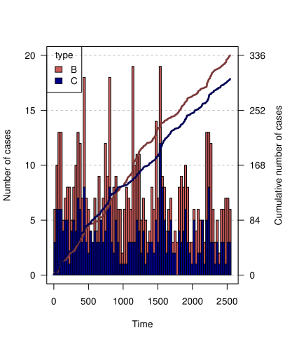
(a)

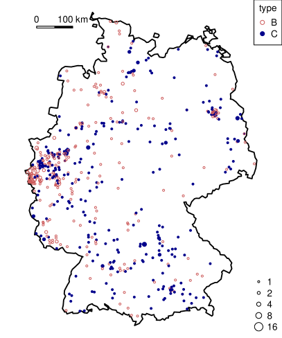
(b)

Figure 2: Occurrence of the two finetypes viewed in the temporal and spatial dimensions.

The time-series plot (Figure LABEL:fig:imdepi_plot1) shows the monthly aggregated number of cases by finetype in a stacked histogram as well as each type’s cumulative number over time. The spatial plot (Figure LABEL:fig:imdepi_plot2) shows the observation window W with the locations of all cases (by type), where the areas of the points are proportional to the number of cases at the respective location. Additional shading by the population is possible and exemplified in help("plot.epidataCS").

The above static plots do not capture the space-time dynamics of epidemic spread. An animation may provide additional insight and can be produced by the corresponding animate-method. For instance, to look at the first year of the B-type in a weekly sequence of snapshots in a web browser (using facilities of the animation package of Xie, 2013):

R> animation::saveHTML(+    animate(subset(imdepi, type == "B"), interval = c(0, 365), time.spacing = 7),+    nmax = Inf, interval = 0.2, loop = FALSE,+    title = "Animation of the first year of type B events") Selecting events from epidataCS as for the animation above is enabled by the [- and subset-methods, which return a new epidataCS object containing only the selected events.

A limited data sampling resolution may lead to tied event times or locations, which are in conflict with a continuous spatio-temporal point process model. For instance, a temporal residual analysis would suggest model deficiencies (Meyer et al., 2012, Figure 4), and a power-law kernel for spatial interaction may diverge if there are events with zero distance to potential source events (Meyer and Held, 2014a). The function untie breaks ties by random shifts. This has already been applied to the event times in the provided imdepi data by subtracting a U(0,1)-distributed random number from the original dates. The event coordinates in the IMD data are subject to interval censoring at the level of Germany’s postcode regions. A possible replacement for the given centroids would thus be a random location within the corresponding postcode area. Lacking a suitable shapefile, Meyer and Held (2014a) shifted all locations by a random vector with length up to half the observed minimum spatial separation:

R> eventDists <- dist(coordinates(imdepi$events))R> (minsep <- min(eventDists[eventDists > 0]))

[1] 1.17

R> set.seed(321)R> imdepi_untied <- untie(imdepi, amount = list(s = minsep / 2)) Note that random tie-breaking requires sensitivity analyses as discussed by Meyer and Held (2014a), but skipped here for the sake of brevity.

The update-method is useful to change the values of the maximum interaction ranges eps.t and eps.s, since it takes care of the necessary updates of the hidden auxiliary variables in an epidataCS object. For an unbounded interaction radius:

R> imdepi_untied_infeps <- update(imdepi_untied, eps.s = Inf)

Last but not least, epidataCS can be converted to the other classes epidata (Section 4) and sts (Section 5) by aggregation. The method as.epidata.epidataCS aggregates events by region (tile), and the function epidataCS2sts yields counts by region and time interval. The data could then, e.g., be analyzed by the multivariate time-series model presented in Section 5. We can also use visualization tools of the sts class, e.g., to produce Figure 3:

R> imdsts <- epidataCS2sts(imdepi, freq = 12, start = c(2002, 1), tiles = districtsD)R> plot(imdsts, type = observed ~ time)R> plot(imdsts, type = observed ~ unit, population = districtsD$POPULATION / 100000)

(a)

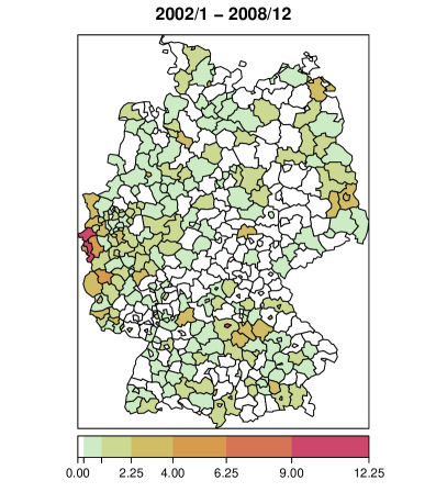
(b)

Figure 3: IMD cases (joint types) aggregated as an sts object by month and district.

3.3 Modeling and inference

Having prepared the data as an object of class epidataCS, the function twinstim can be used to perform likelihood inference for conditional intensity models of the form (2). The main arguments for twinstim are the formulae of the endemic and epidemic linear predictors ($\nu_{[\bm{s}][t]}=\exp$(endemic) and $\eta_{j}=\exp$(epidemic)), and the spatial and temporal interaction functions siaf ($f$) and tiaf ($g$), respectively. Both formulae are parsed internally using the standard model.frame toolbox from package stats and thus can handle factor variables and interaction terms. While the endemic linear predictor incorporates time-dependent and/or areal-level covariates from stgrid, the epidemic formula may use both stgrid variables and event marks to be associated with the force of infection. For the interaction functions, several alternatives are predefined as listed in Table 3. They are applicable out-of-the-box and illustrated as part of the following modeling exercise for the IMD data. Own interaction functions can also be used provided their implementation obeys a certain structure, see help("siaf") and help("tiaf"), respectively.

Spatial (siaf.*)	Temporal (tiaf.*)
constant	constant
gaussian	exponential
powerlaw	step
powerlawL
step
student

Table 3: Predefined spatial and temporal interaction functions.

3.3.1 Basic example

To illustrate statistical inference with twinstim, we will estimate several models for the simplified and “untied” IMD data presented in Section 3.2. In the endemic component, we include the district-specific population density as a multiplicative offset, a (centered) time trend, and a sinusoidal wave of frequency $2\pi/365$ to capture seasonality, where the start variable from stgrid measures time:

R> (endemic <- addSeason2formula(~offset(log(popdensity)) + I(start / 365 - 3.5),+    period = 365, timevar = "start"))

~offset(log(popdensity)) + I(start/365 - 3.5) + sin(2 * pi *    start/365) + cos(2 * pi * start/365) See Held and Paul (2012, Section 2.2) for how such sine/cosine terms reflect seasonality. Because of the aforementioned integrations in the log-likelihood (5), it is advisable to first fit an endemic-only model to obtain reasonable start values for more complex epidemic models:

R> imdfit_endemic <- twinstim(endemic = endemic, epidemic = ~0,+    data = imdepi_untied, subset = !is.na(agegrp)) We exclude the single case with unknown age group from this analysis since we will later estimate an effect of the age group on the force of infection.

Display	Extract	Modify	Other
print	nobs	update	simulate
summary	vcov	add1	epitest
xtable	coeflist	drop1
plot	logLik	stepComponent
intensityplot	extractAIC
iafplot	profile
checkResidualProcess	residuals
	terms
	R0

Table 4: Generic and non-generic functions applicable to twinstim objects. Note that there is no need for specific coef, confint, AIC or BIC methods, since the respective default methods from package stats apply outright.

Many of the standard functions to access model fits in R are also implemented for twinstim fits (see Table 4). For example, we can produce the usual model summary:

R> summary(imdfit_endemic)

Call:twinstim(endemic = endemic, epidemic = ~0, data = imdepi_untied,    subset = !is.na(agegrp))Coefficients of the endemic component:                          Estimate Std. Error z value Pr(>|z|)h.(Intercept)             -20.3683     0.0419 -486.24  < 2e-16 ***h.I(start/365 - 3.5)       -0.0444     0.0200   -2.22    0.027 *h.sin(2 * pi * start/365)   0.2733     0.0576    4.75  2.0e-06 ***h.cos(2 * pi * start/365)   0.3509     0.0581    6.04  1.5e-09 ***---Signif. codes:  0 ’***’ 0.001 ’**’ 0.01 ’*’ 0.05 ’.’ 0.1 ’ ’ 1No epidemic component.AIC:  19166Log-likelihood: -9579

Because of the aforementioned equivalence of the endemic component with a Poisson regression model, the coefficients can be interpreted as log rate ratios in the usual way. For instance, the endemic rate is estimated to decrease by 1 - exp(coef(imdfit_endemic)[2]) $=$ 4.3% per year. Coefficient correlations can be retrieved by the argument correlation = TRUE in the summary call just like for summary.glm, but may also be extracted via the standard cov2cor(vcov(imdfit_endemic)).

We now update the endemic model to take additional spatio-temporal dependence between events into account. Infectivity shall depend on the meningococcal finetype and the age group of the patient, and is assumed to be constant over time (default), $g(t)=\mathbbm{1}_{(0,30]}(t)$, with a Gaussian distance-decay $f(x)=\exp\left\{-x^{2}/(2\sigma^{2})\right\}$. This model was originally selected by Meyer et al. (2012) and can be fitted as follows:

R> imdfit_Gaussian <- update(imdfit_endemic, epidemic = ~type + agegrp,+    siaf = siaf.gaussian(), start = c("e.(Intercept)" = -12.5, "e.siaf.1" = 2.75),+    control.siaf = list(F = list(adapt = 0.25), Deriv = list(nGQ = 13)),+    cores = 2 * (.Platform$OS.type == "unix"), model = TRUE) To reduce the runtime of this example, we specified convenient start values for some parameters (others start at 0) and set control.siaf with a rather low number of nodes for the cubature of $f(\lVert\bm{s}\rVert)$ in the log-likelihood (via the midpoint rule) and $\frac{\partial f(\lVert\bm{s}\rVert)}{\partial\log\sigma}$ in the score function (via product Gauss cubature). On Unix-alikes, these numerical integrations can be performed in parallel using the “multicore” functions mclapply et al. from the base package parallel, here with cores = 2 processes. For later generation of an intensityplot, the model environment is retained.

	RR	95% CI	p-value
h.I(start/365 - 3.5)	0.955	0.91–1.00	0.039
h.sin(2 * pi * start/365)	1.243	1.09–1.41	0.0008
h.cos(2 * pi * start/365)	1.375	1.21–1.56	$<$0.0001
e.typeC	0.402	0.24–0.68	0.0007
e.agegrp[3,19)	2.000	1.06–3.78	0.033
e.agegrp[19,Inf)	0.776	0.32–1.91	0.58

Table 5: Estimated rate ratios (RR) and associated Wald confidence intervals (CI) for endemic (h.) and epidemic (e.) terms. This table was generated by xtable(imdfit_Gaussian).

Table 5 shows the output of twinstim’s xtable method (Dahl, 2015), which provides rate ratios for the endemic and epidemic effects. The alternative toLatex method simply translates the summary table of coefficients to LaTeX without exp-transformation. On the subject-matter level, we can conclude from Table 5 that the meningococcal finetype of serogroup C is less than half as infectious as the B-type, and that patients in the age group 3 to 18 years are estimated to cause twice as many secondary infections as infants aged 0 to 2 years.

3.3.2 Model-based effective reproduction numbers

The event-specific reproduction numbers (3) can be extracted from fitted twinstim objects via the R0 method. For the above IMD model, we obtain the following mean numbers of secondary infections by finetype:

R> R0_events <- R0(imdfit_Gaussian)R> tapply(R0_events, marks(imdepi_untied)[names(R0_events), "type"], mean)

     B      C0.2161 0.0958 Confidence intervals can be obtained via Monte Carlo simulation, where Equation 3 is repeatedly evaluated with parameters sampled from the asymptotic multivariate normal distribution of the maximum likelihood estimate. For this purpose, the R0-method takes an argument newcoef, which is exemplified in help("R0").

3.3.3 Interaction functions

Figure 4 shows several estimated spatial interaction functions, which can be plotted by, e.g., plot(imdfit_Gaussian, which = "siaf"). Meyer and Held (2014a) found that a power-law decay of spatial interaction is more appropriate than a Gaussian kernel to describe the spread of human infectious diseases. The power-law kernel concentrates on short-range interaction, but also exhibits a heavier tail reflecting occasional transmission over large distances. To use the power-law kernel $f(x)=(x+\sigma)^{-d}$, we switch to the prepared epidataCS object with eps.s = Inf and update the previous Gaussian model as follows:

R> imdfit_powerlaw <- update(imdfit_Gaussian, data = imdepi_untied_infeps,+    siaf = siaf.powerlaw(), control.siaf = NULL,+    start = c("e.(Intercept)" = -6.2, "e.siaf.1" = 1.5, "e.siaf.2" = 0.9))

Table 3 also lists the step function kernel as an alternative, which is particularly useful for two reasons. First, it is a more flexible approach since it estimates interaction between the given knots without assuming an overall functional form. Second, the spatial integrals in the log-likelihood can be computed analytically for the step function kernel, which therefore offers a quick estimate of spatial interaction. We update the Gaussian model to use four steps at log-equidistant knots up to an interaction range of 100 km:

R> imdfit_step4 <- update(imdfit_Gaussian, data = imdepi_untied_infeps,+    siaf = siaf.step(exp(1:4 * log(100) / 5), maxRange = 100), control.siaf = NULL,+    start = c("e.(Intercept)" = -10, setNames(-2:-5, paste0("e.siaf.", 1:4)))) Figure 4 suggests that the estimated step function is in line with the power law.

For the temporal interaction function $g(t)$, model updates and plots are similarly possible, e.g., update(imdfit_Gaussian, tiaf = tiaf.exponential()). However, the events in the IMD data are too rare to infer the time-course of infectivity with confidence.

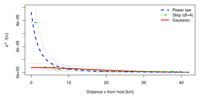
Figure 4: Various estimates of spatial interaction (scaled by the epidemic intercept $\gamma_{0}$). The standard deviation of the Gaussian kernel is estimated to be $\hat{\sigma}=$ 16.00 (95% CI: 13.65–18.75), and the estimated power-law parameters are $\hat{\sigma}=$ 4.64 (95% CI: 1.82–11.84) and $\hat{d}=$ 2.49 (95% CI: 1.81–3.42).

3.3.4 Model selection

R> AIC(imdfit_endemic, imdfit_Gaussian, imdfit_powerlaw, imdfit_step4)

                df   AICimdfit_endemic   4 19166imdfit_Gaussian  9 18967imdfit_powerlaw 10 18940imdfit_step4    12 18933

Akaike’s Information Criterion (AIC) suggests superiority of the power-law vs. the Gaussian model and the endemic-only model. The more flexible step function yields the best AIC value but its shape strongly depends on the chosen knots and is not guaranteed to be monotonically decreasing. The function stepComponent – a wrapper around the step function from stats – can be used to perform AIC-based stepwise selection within a given model component.

3.3.5 Model diagnostics

Two other plots are implemented for twinstim objects. Figure 5 shows an intensityplot of the fitted “ground” intensity $\sum_{k=1}^{2}\int_{\bm{W}}\hat{\lambda}(\bm{s},t,k)\,\mathrm{d}\bm{s}$ aggregated over both event types:

R> intensityplot(imdfit_powerlaw, which = "total", aggregate = "time", types = 1:2)

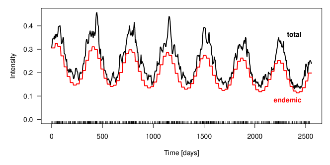
Figure 5: Fitted “ground” intensity process aggregated over space and both types.

The estimated endemic intensity component has also been added to the plot. It exhibits strong seasonality and a slow negative trend. The proportion of the endemic intensity is rather constant along time since no major outbreaks occurred. This proportion can be visualized separately by specifying which = "endemic proportion" in the above call.

Spatial intensityplots can be produced via aggregate = "space" and require a geographic representation of stgrid. Figure 6 shows the accummulated epidemic proportion by event type. It is naturally high in regions with a large number of cases and even more so if the population density is low. The function epitest offers a model-based global test for epidemicity, while knox and stKtest implement related classical approaches (Meyer et al., 2015).

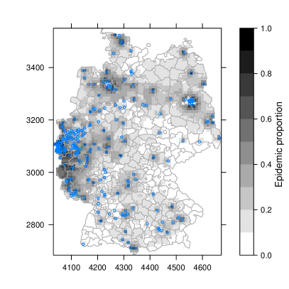
(a)

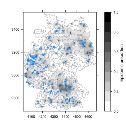
(b)

Figure 6: Epidemic proportion of the fitted intensity process accumulated over time by type.

Another diagnostic tool is the function checkResidualProcess, which transforms the temporal “residual process” in such a way that it exhibits a uniform distribution and lacks serial correlation if the fitted model describes the true CIF well (see Ogata, 1988, Section 3.3). These properties can be checked graphically as in Figure 7 produced by:

R> checkResidualProcess(imdfit_powerlaw)

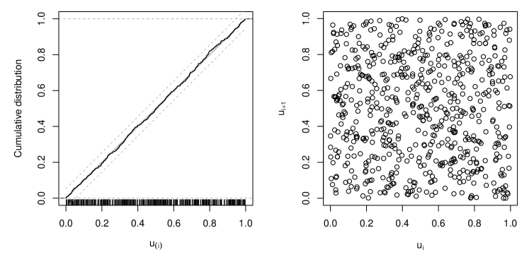
Figure 7: The left plot shows the ecdf of the transformed residuals with a 95% confidence band obtained by inverting the corresponding Kolmogorov-Smirnov test (no evidence for deviation from uniformity). The right-hand plot suggests absence of serial correlation.

3.4 Simulation

To identify regions with unexpected IMD dynamics, Meyer et al. (2012) compared the observed numbers of cases by district to the respective 2.5% and 97.5% quantiles of 100 simulations from the selected model. Furthermore, simulations allow us to investigate the stochastic volatility of the endemic-epidemic process, to obtain probabilistic forecasts, and to perform parametric bootstrap of the spatio-temporal point pattern.

The simulation algorithm we apply is described in Meyer et al. (2012, Section 4). It requires a geographic representation of the stgrid, as well as functionality for sampling locations from the spatial kernel $f_{2}(\bm{s}):=f(\lVert\bm{s}\rVert)$. This is implemented for all predefined spatial interaction functions listed in Table 3. Event marks are by default sampled from their respective empirical distribution in the original data. The following code runs 30 simulations over the last two years based on the estimated power-law model:

R> imdsims <- simulate(imdfit_powerlaw, nsim = 30, seed = 1, t0 = 1826, T = 2555,+    data = imdepi_untied_infeps, tiles = districtsD) Figure 8 shows the cumulative number of cases from the simulations appended to the first five years of data. Extracting a single simulation (e.g., imdsims[[1]]) yields an object of the class simEpidataCS, which extends epidataCS. It carries additional components from the generating model to enable an R0-method and intensityplots for simulated data. A special feature of such simulations is that the source of each event is actually known:

R> table(imdsims[[1]]$events$source > 0, exclude = NULL)

FALSE  TRUE  <NA>  112    25     8 The stored source value is 0 for endemic events, NA for events of the prehistory but still infective at t0, and otherwise corresponds to the row index of the infective source. Averaged over all 30 simulations, the proportion of events triggered by previous events is 0.218.

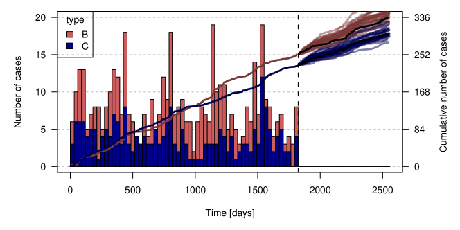
Figure 8: Simulation-based forecast of the cumulative number of cases by finetype in the last two years. The black lines correspond to the observed numbers.

4 SIR event history of a fixed population

The endemic-epidemic multivariate point process model “twinSIR” is designed for individual-level surveillance data of a fixed population of which the complete SIR event history is assumed to be known. As an illustrative example, we use a particularly well-documented measles outbreak among children of the isolated German village Hagelloch in the year 1861, which has previously been analyzed by, e.g., Neal and Roberts (2004). Other potential applications include farm-level data as well as epidemics across networks. We start by describing the general model class in Section 4.1. Section 4.2 introduces the example data and the associated class epidata, and Section 4.3 presents the core functionality of fitting and analyzing such data using twinSIR. Due to the many similarities with the twinstim framework covered in Section 3, we condense the twinSIR treatment accordingly.

4.1 Model class: twinSIR

The previously described point process model twinstim (Section 3) is indexed in a continuous spatial domain, i.e., the set of possible event locations consists of the whole observation region and is thus infinite. However, if infections can only occur at a known discrete set of sites, such as for livestock diseases among farms, the conditional intensity function formally becomes $\lambda_{i}(t)$. It characterizes the instantaneous rate of infection of individual $i$ at time $t$, given the sets $S(t)$ and $I(t)$ of susceptible and infectious individuals, respectively (just before time $t$). In a similar regression view as in Section 3, Höhle (2009) proposed the endemic-epidemic multivariate temporal point process “twinSIR”:

$$\lambda_{i}(t)=\lambda_{0}(t)\,\nu_{i}(t)+\sum_{j\in I(t)}\left\{f(d_{ij})+\bm{w}_{ij}^{\top}\bm{\alpha}^{(w)}\right\}\>,$$ (6)

if $i\in S(t)$, i.e., if individual $i$ is currently susceptible, and $\lambda_{i}(t)=0$ otherwise. The rate decomposes into two components. The endemic component consists of a Cox proportional hazards formulation containing a semi-parametric baseline hazard $\lambda_{0}(t)$ and a log-linear predictor $\nu_{i}(t)=\exp\left(\bm{z}_{i}(t)^{\top}\bm{\beta}\right)$ of covariates modeling infection from external sources. Furthermore, an additive epidemic component captures transmission from the set $I(t)$ of currently infectious individuals. The force of infection of individual $i$ depends on the distance $d_{ij}$ to each infective source $j\in I(t)$ through a distance kernel

$$f(u)=\sum_{m=1}^{M}\alpha_{m}^{(f)}B_{m}(u)\>\geq 0\>,$$ (7)

which is represented by a linear combination of non-negative basis functions $B_{m}$ with the $\alpha_{m}^{(f)}$’s being the respective coefficients. For instance, $f$ could be modelled by a B-spline (Fahrmeir et al., 2013, Section 8.1), and $d_{ij}$ could refer to the Euclidean distance $\lVert\bm{s}_{i}-\bm{s}_{j}\rVert$ between the individuals’ locations $\bm{s}_{i}$ and $\bm{s}_{j}$, or to the geodesic distance between the nodes $i$ and $j$ in a network. The distance-based force of infection is modified additively by a linear predictor of covariates $\bm{w}_{ij}$ describing the interaction of individuals $i$ and $j$ further. Hence, the whole epidemic component of Equation 6 can be written as a single linear predictor $\bm{x}_{i}(t)^{\top}\bm{\alpha}$ by interchanging the summation order to

$$\sum_{m=1}^{M}\alpha^{(f)}_{m}\sum_{j\in I(t)}B_{m}(d_{ij})+\sum_{k=1}^{K}\alpha^{(w)}_{k}\sum_{j\in I(t)}w_{ijk}=\bm{x}_{i}(t)^{\top}\bm{\alpha}\>,$$ (8)

such that $\bm{x}_{i}(t)$ comprises all epidemic terms summed over $j\in I(t)$. Note that the use of additive covariates $\bm{w}_{ij}$ on top of the distance kernel in (6) is different from twinstim’s multiplicative approach in (2). One advantage of the additive approach is that the subsequent linear decomposition of the distance kernel allows one to gather all parts of the epidemic component in a single linear predictor. Hence, the above model represents a CIF extension of what in the context of survival analysis is known as an additive-multiplicative hazard model (Martinussen and Scheike, 2002). As a consequence, the twinSIR model could in principle be fitted with the timereg package (Scheike and Martinussen, 2006), which yields estimates for the cumulative hazards. However, Höhle (2009) chooses a more direct inferential approach: To ensure that the CIF $\lambda_{i}(t)$ is non-negative, all covariates are encoded such that the components of $\bm{w}_{ij}$ are non-negative. Additionally, the parameter vector $\bm{\alpha}$ is constrained to be non-negative. Subsequent parameter inference is then based on the resulting constrained penalized likelihood which gives directly interpretable estimates of $\bm{\alpha}$.

4.2 Data structure: epidata

New SIR-type event data typically arrive in the form of a simple data frame with one row per individual and the time points of the sequential events of the individual as columns. For the 1861 Hagelloch measles epidemic, such a data set of the 188 affected children is contained in the surveillance package:

R> data("hagelloch")R> head(hagelloch.df, n = 5)

  PN    NAME FN HN AGE    SEX        PRO        ERU        CL DEAD IFTO SI1  1 Mueller 41 61   7 female 1861-11-21 1861-11-25 1st class <NA>   45 102  2 Mueller 41 61   6 female 1861-11-23 1861-11-27 1st class <NA>   45 123  3 Mueller 41 61   4 female 1861-11-28 1861-12-02 preschool <NA>  172  94  4 Seibold 61 62  13   male 1861-11-27 1861-11-28 2nd class <NA>  180 105  5  Motzer 42 63   8 female 1861-11-22 1861-11-27 1st class <NA>   45 11                C PR CA NI GE TD   TM x.loc y.loc tPRO tERU tDEAD   tR   tI1 no complicatons  4  4  3  1 NA   NA   142   100 22.7 26.2    NA 29.2 21.72 no complicatons  4  4  3  1  3 40.3   142   100 24.2 28.8    NA 31.8 23.23 no complicatons  4  4  3  2  1 40.5   142   100 29.6 33.7    NA 36.7 28.64 no complicatons  1  1  1  1  3 40.7   165   102 28.1 29.0    NA 32.0 27.15 no complicatons  5  3  2  1 NA   NA   145   120 23.1 28.4    NA 31.4 22.1 The help("hagelloch") contains a description of all columns. Here we concentrate on the event columns PRO (appearance of prodromes), ERU (eruption), and DEAD (day of death if during the outbreak). We take the day on which the index case developed first symptoms, 30 October 1861 (min(hagelloch.df$PRO)$), as the start of the epidemic, i.e., we condition on this case being initially infectious. As for twinstim, the property of point processes that concurrent events have zero probability requires special treatment. Ties are due to the interval censoring of the data to a daily basis – we broke these ties by adding random jitter to the event times within the given days. The resulting columns tPRO, tERU, and tDEAD are relative to the defined start time. Following Neal and Roberts (2004), we assume that each child becomes infectious (S $\rightarrow$ I event at time tI) one day before the appearance of prodromes, and is removed from the epidemic (I $\rightarrow$ R event at time tR) three days after the appearance of rash or at the time of death, whichever comes first.

For further processing of the data, we convert hagelloch.df to the standardized epidata structure for twinSIR. This is done by the converter function as.epidata, which also checks consistency and optionally pre-calculates the epidemic terms $\bm{x}_{i}(t)$ of Equation 8 to be incorporated in a twinSIR model. The following call generates the epidata object hagelloch:

R> hagelloch <- as.epidata(hagelloch.df,+    t0 = 0, tI.col = "tI", tR.col = "tR",+    id.col = "PN", coords.cols = c("x.loc", "y.loc"),+    f = list(household    = function(u) u == 0,+             nothousehold = function(u) u > 0),+    w = list(c1 = function (CL.i, CL.j) CL.i == "1st class" & CL.j == CL.i,+             c2 = function (CL.i, CL.j) CL.i == "2nd class" & CL.j == CL.i),+    keep.cols = c("SEX", "AGE", "CL")) The coordinates (x.loc, y.loc) correspond to the location of the household the child lives in and are measured in meters. Note that twinSIR allows for tied locations of individuals, but assumes the relevant spatial location to be fixed during the entire observation period. By default, the Euclidean distance between the given coordinates will be used. Alternatively, as.epidata also accepts a pre-computed distance matrix via its argument D without requiring spatial coordinates. The argument f lists distance-dependent basis functions $B_{m}$ for which the epidemic terms $\sum_{j\in I(t)}B_{m}(d_{ij})$ shall be generated. Here, household ($x_{i,H}(t)$) and nothousehold ($x_{i,\bar{H}}(t)$) count for each child the number of currently infective children in its household and outside its household, respectively. Similar to Neal and Roberts (2004), we also calculate the covariate-based epidemic terms c1 ($x_{i,c1}(t)$) and c2 ($x_{i,c2}(t)$) counting the number of currently infective classmates. Note from the corresponding definitions of $w_{ij1}$ and $w_{ij2}$ in w that c1 is always zero for children of the second class and c2 is always zero for children of the first class. For pre-school children, both variables equal zero over the whole period. By the last argument keep.cols, we choose to only keep the covariates SEX, AGE, and school CLass from hagelloch.df.

The first few rows of the generated epidata object are shown below:

R> head(hagelloch, n = 5)

  BLOCK id start stop atRiskY event Revent x.loc y.loc    SEX AGE        CL1     1  1     0 1.14       1     0      0   142   100 female   7 1st class2     1  2     0 1.14       1     0      0   142   100 female   6 1st class3     1  3     0 1.14       1     0      0   142   100 female   4 preschool4     1  4     0 1.14       1     0      0   165   102   male  13 2nd class5     1  5     0 1.14       1     0      0   145   120 female   8 1st class  household nothousehold c1 c21         0            1  0  02         0            1  0  03         0            1  0  04         0            1  0  15         0            1  0  0

The epidata structure inherits from counting processes as implemented by the Surv class of package survival (Therneau, 2015) and also used in, e.g., the timereg package (Scheike and Zhang, 2011). Specifically, the observation period is splitted up into consecutive time intervals (start; stop] of constant conditional intensities. As the CIF $\lambda_{i}(t)$ of Equation (6) only changes at time points, where the set of infectious individuals $I(t)$ or some endemic covariate in $\nu_{i}(t)$ change, those occurrences define the break points of the time intervals. Altogether, the hagelloch event history consists of 375 time BLOCKs of 188 rows, where each row describes the state of individual id during the corresponding time interval. The susceptibility status and the I- and R-events are captured by the columns atRiskY, event and Revent, respectively. The atRiskY column indicates if the individual is at risk of becoming infected in the current interval. The event columns indicate, which individual was infected or removed at the stop time. Note that at most one entry in the event and Revent columns is 1, all others are 0.

Apart from being the input format for twinSIR models, the epidata class has several associated methods (Table 6), which are similar in spirit to the methods described for epidataCS.

Display	Subset	Modify
print	[	update
summary
plot
animate
stateplot

Table 6: Generic and non-generic functions applicable to epidata objects.

For example, Figure 9 illustrates the course of the Hagelloch measles epidemic by counting processes for the number of susceptible, infectious and removed children, respectively. Figure 10 shows the locations of the households. An animated map can also be produced to view the households’ states over time and a stateplot shows the changes for a selected unit.

R> plot(hagelloch, xlab = "Time [days]")

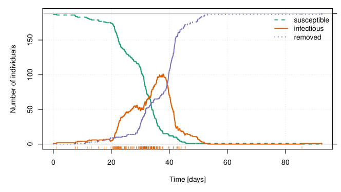
Figure 9: Evolution of the 1861 Hagelloch measles epidemic in terms of the numbers of susceptible, infectious, and recovered children. The bottom rug marks the infection times tI.

R> hagelloch_coords <- summary(hagelloch)$coordinatesR> plot(hagelloch_coords, xlab = "x [m]", ylab = "y [m]",+    pch = 15, asp = 1, cex = sqrt(multiplicity(hagelloch_coords)))R> legend(x = "topleft", pch = 15, legend = c(1, 4, 8), pt.cex = sqrt(c(1, 4, 8)),+    title = "Household size")

Figure 10: Spatial locations of the Hagelloch households. The size of each dot is proportional to the number of children in the household.

4.3 Modeling and inference

4.3.1 Basic example

To illustrate the flexibility of twinSIR we will analyze the Hagelloch data using class room and household indicators similar to Neal and Roberts (2004). We include an additional endemic background rate $\exp(\beta_{0})$, which allows for multiple outbreaks triggered by external sources. Consequently, we do not need to ignore the child that got infected about one month after the end of the main epidemic (see the last event mark in Figure 9), as, e.g., done in a thorough network-based analysis of the Hagelloch data by Groendyke et al. (2012). Altogether, the CIF for a child $i$ is modeled as

$$\lambda_{i}(t)=Y_{i}(t)\cdot\left[\exp(\beta_{0})+\alpha_{H}x_{i,H}(t)+\alpha_{c1}x_{i,c1}(t)+\alpha_{c2}x_{i,c2}(t)+\alpha_{\bar{H}}x_{i,\bar{H}}(t)\right]\>,$$ (9)

where $Y_{i}(t)=\mathbbm{1}(i\in S(t))$ is the at-risk indicator. By counting the number of infectious classmates separately for both school classes as described in the previous section, we allow for class-specific effects $\alpha_{c1}$ and $\alpha_{c2}$ on the force of infection. The model is estimated by maximum likelihood (Höhle, 2009) using the following call:

R> hagellochFit <- twinSIR(~household + c1 + c2 + nothousehold, data = hagelloch)R> summary(hagellochFit)

Call:twinSIR(formula = ~household + c1 + c2 + nothousehold, data = hagelloch)Coefficients:                  Estimate Std. Error z value Pr(>|z|)household         0.026868   0.006113    4.39  1.1e-05 ***c1                0.023892   0.005026    4.75  2.0e-06 ***c2                0.002932   0.000755    3.88   0.0001 ***nothousehold      0.000831   0.000142    5.87  4.3e-09 ***cox(logbaseline) -7.362644   0.887989   -8.29  < 2e-16 ***---Signif. codes:  0 ’***’ 0.001 ’**’ 0.01 ’*’ 0.05 ’.’ 0.1 ’ ’ 1Total number of infections:  187One-sided AIC: 1245(simulated penalty weights)Log-likelihood: -619Number of log-likelihood evaluations: 119

The results show, e.g., a 0.0239 / 0.0029 $=$ 8.15 times higher transmission between individuals in the 1st class than in the 2nd class. Furthermore, an infectious housemate adds 0.0269 / 0.0008 $=$ 32.3 times as much infection pressure as infectious children outside the household. The endemic background rate of infection in a population with no current measles cases is estimated to be $\exp(\hat{\beta}_{0})=\exp(-7.36)=0.000635$. An associated Wald confidence interval (CI) based on the asymptotic normality of the maximum likelihood estimator (MLE) can be obtained by exp-transforming the confint for $\beta_{0}$:

R> exp(confint(hagellochFit, parm = "cox(logbaseline)"))

                    2.5 %  97.5 %cox(logbaseline) 0.000111 0.00362

Note that Wald confidence intervals for the epidemic parameters $\bm{\alpha}$ are to be treated carefully, because their construction does not take the restricted parameter space into account. For more adequate statistical inference, the behavior of the log-likelihood near the MLE can be investigated using the profile-method for twinSIR objects. For instance, to evaluate the normalized profile log-likelihood of $\alpha_{c1}$ and $\alpha_{c2}$ on an equidistant grid of 25 points within the corresponding 95% Wald CIs, we do:

R> prof <- profile(hagellochFit,+    list(c(match("c1", names(coef(hagellochFit))), NA, NA, 25),+         c(match("c2", names(coef(hagellochFit))), NA, NA, 25))) The profiling result contains 95% highest likelihood based CIs for the parameters, as well as the Wald CIs for comparison:

R> prof$ci.hl

   idx  hl.low   hl.up wald.low wald.up     mlec1   2 0.01522 0.03497  0.01404 0.03374 0.02389c2   3 0.00158 0.00454  0.00145 0.00441 0.00293 The entire functional form of the normalized profile log-likelihood on the requested grid as stored in prof$lp$ can be visualized by:

R> plot(prof)

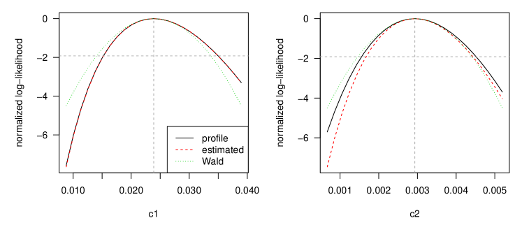
Figure 11: Normalized log-likelihood for $\alpha_{c1}$ and $\alpha_{c2}$ when fitting the twinSIR model formulated in Equation (9) to the Hagelloch data.

4.3.2 Model diagnostics

Display	Extract	Other
print	vcov	simulate
summary	logLik
plot	AIC
intensityplot	extractAIC
checkResidualProcess	profile
	residuals

Table 7: Generic and non-generic functions for twinSIR. There are no specific coef or confint methods, since the respective default methods from package stats apply outright.

Table 7 lists all methods for the twinSIR class. For example, to investigate how the CIF decomposes into endemic and epidemic intensity over time, we produce Figure LABEL:fig:hagellochFit_plot1 by:

R> plot(hagellochFit, which = "epidemic proportion", xlab = "time [days]")

(a)

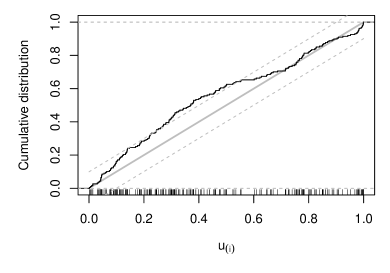
(b)

Figure 12: Diagnostic plots for the twinSIR model formulated in Equation 9.

Note that the last infection was necessarily caused by the endemic component since there were no more infectious children in the observed population which could have triggered the new case. We can also inspect temporal Cox-Snell-like residuals of the fitted point process using the function checkResidualProcess as for the spatio-temporal point process models in Section 3.3. The resulting Figure LABEL:fig:hagellochFit_plot2 reveals some deficiencies of the model in describing the waiting times between events, which might be related to the assumption of fixed infection periods.

Finally, twinSIR’s AIC-method computes the one-sided AIC (Hughes and King, 2003) as described in Höhle (2009), which can be used for model selection under positivity constraints on $\bm{\alpha}$. For instance, we may consider a more flexible model for local spread using a step function for the distance kernel $f(u)$ in Equation 7. An updated model with $B_{1}=I_{(0;100)}(u)$, $B_{2}=I_{[100;200)}(u)$, $B_{3}=I_{[200;\infty)}(u)$ can be fitted as follows:

R> knots <- c(100, 200)R> fstep <- list(+    B1 = function(D) D > 0 & D < knots[1],+    B2 = function(D) D >= knots[1] & D < knots[2],+    B3 = function(D) D >= knots[2])R> hagellochFit_fstep <- twinSIR(+    ~household + c1 + c2 + B1 + B2 + B3,+    data = update(hagelloch, f = fstep))

R> set.seed(1)R> AIC(hagellochFit, hagellochFit_fstep)

                   df  AIChagellochFit        5 1245hagellochFit_fstep  7 1246 Hence the simpler model with just a nothousehold component instead of the more flexible distance-based step function is preferred. A random seed was set since the parameter penalty in the one-sided AIC is determined by Monte Carlo simulation. The algorithm is described in Silvapulle and Sen (2005, p. 79, Simulation 3) and involves quadratic programming using package quadprog (Turlach, 2013).

4.4 Simulation

Simulation from fitted twinSIR models is described in detail in Höhle (2009, Section 4). The implementation is made available by an appropriate simulate-method for class twinSIR. Because both the algorithm and the call are similar to the invocation on twinstim objects (Section 3.4), we skip the illustration here and refer to help("simulate.twinSIR").

5 Areal time series of counts

In public health surveillance, routine reports of infections to public health authorities give rise to spatio-temporal data, which are usually made available in the form of aggregated counts by region and period. The Robert Koch Institute (RKI) in Germany, for example, maintains a database of cases of notifiable diseases, which can be queried via the SurvStat@RKI online service. As an illustrative example, we use weekly counts of measles infections by district in the Weser-Ems region of Lower Saxony, Germany, 2001–2002. These spatio-temporal count data constitute the response $Y_{it}$, $i=1,\dotsc,17$ (districts), $t=1,\dotsc,104$ (weeks), for our illustration of the endemic-epidemic multivariate time-series model “hhh4”. We start by describing the general model class in Section 5.1. Section 5.2 introduces the data and the associated S4-class sts (“surveillance time series”). In Section 5.3, a simple model for the measles data based on the original analysis of Held et al. (2005) is introduced, which is then sequentially improved by suitable model extensions. The final Section 5.4 illustrates simulation from fitted hhh4 models.

5.1 Model class: hhh4

An endemic-epidemic multivariate time-series model for infectious disease counts $Y_{it}$ from units $i=1,\dotsc,I$ during periods $t=1,\dotsc,T$ was proposed by Held et al. (2005) and was later extended in a series of papers (Paul et al., 2008; Paul and Held, 2011; Held and Paul, 2012; Meyer and Held, 2014a). In its most general formulation, this so-called “hhh4” model assumes that, conditional on past observations, $Y_{it}$ has a negative binomial distribution with mean

$$\mu_{it}=e_{it}\,\nu_{it}+\lambda_{it}\,Y_{i,t-1}+\phi_{it}\sum_{j\neq i}w_{ji}\,Y_{j,t-1}$$ (10)

and overdispersion parameter $\psi_{i}>0$ such that the conditional variance of $Y_{it}$ is $\mu_{it}(1+\psi_{i}\mu_{it})$. Shared overdispersion parameters, e.g., $\psi_{i}\equiv\psi$, are supported as well as replacing the negative binomial by a Poisson distribution, which corresponds to the limit $\psi_{i}\equiv 0$.

Similar to the point process models of Sections 3 and 4, the mean (10) decomposes additively into endemic and epidemic components. The endemic mean is usually modelled proportional to an offset of expected counts $e_{it}$. In spatial applications of the multivariate hhh4 model as in this paper, the “unit” $i$ refers to a geographical region and we typically use (the fraction of) the population living in region $i$ as the endemic offset. The observation-driven epidemic component splits up into autoregressive effects, i.e., reproduction of the disease within region $i$, and neighbourhood effects, i.e., transmission from other regions $j$. Overall, Equation 10 becomes a rich regression model by allowing for log-linear predictors in all three components:

$$\log(\nu_{it}) =\alpha_{i}^{(\nu)}+{\bm{\beta}^{(\nu)}}^{\top}\bm{z}^{(\nu)}_{it}\>,$$ (11)

$$\log(\lambda_{it}) =\alpha_{i}^{(\lambda)}+{\bm{\beta}^{(\lambda)}}^{\top}\bm{z}^{(\lambda)}_{it}\>,$$ (12)

$$\log(\phi_{it}) =\alpha_{i}^{(\phi)}+{\bm{\beta}^{(\phi)}}^{\top}\bm{z}^{(\phi)}_{it}\>.$$ (13)

The intercepts of these predictors can be assumed identical across units, unit-specific, or random (and possibly correlated). The regression terms often involve sine-cosine effects of time to reflect seasonally varying incidence, but may, e.g., also capture heterogeneous vaccination coverage (Herzog et al., 2011). Data on infections imported from outside the study region may enter the endemic component (Geilhufe et al., 2014), which generally accounts for cases not directly linked to other observed cases, e.g., due to edge effects.

For a single time series of counts $Y_{t}$, hhh4 can be regarded as an extension of glm.nb from package MASS (Venables and Ripley, 2002) to account for autoregression. See the vignette("hhh4") for examples of modeling univariate and bivariate count time series using hhh4. With multiple regions, spatio-temporal dependence is adopted by the third component in Equation 10 with weights $w_{ji}$ reflecting the flow of infections from region $j$ to region $i$. These transmission weights may be informed by movement network data (Paul et al., 2008; Schrödle et al., 2012; Geilhufe et al., 2014), but may also be estimated parametrically. A suitable choice to reflect epidemiological coupling between regions (Keeling and Rohani, 2008, Chapter 7) is a power-law distance decay $w_{ji}=o_{ji}^{-d}$ defined in terms of the adjacency order $o_{ji}$ in the neighbourhood graph of the regions (Meyer and Held, 2014a). Note that we usually normalize the transmission weights such that $\sum_{i}w_{ji}=1$, i.e., the $Y_{j,t-1}$ cases are distributed among the regions proportionally to the $j$’th row vector of the weight matrix $(w_{ji})$.

Likelihood inference for the above multivariate time-series model has been established by Paul and Held (2011) with extensions for parametric neighbourhood weights by Meyer and Held (2014a). Supplied with the analytical score function and Fisher information, the function hhh4 by default uses the quasi-Newton algorithm available through the R function nlminb to maximize the log-likelihood. Convergence is usually fast even for a large number of parameters. If the model contains random effects, the penalized and marginal log-likelihoods are maximized alternately until convergence. Computation of the marginal Fisher information is accelerated using the Matrix package (Bates and Maechler, 2015).

5.2 Data structure: sts

We briefly introduce the S4-class sts used for data input in hhh4 models. See Höhle and Mazick (2010) and Salmon et al. (2015) for more detailed descriptions of this class, which is also used for the prospective aberration detection facilities of the surveillance package.

The epidemic modeling of multivariate count time series essentially involves three data matrices: a $T\times I$ matrix of the observed counts, a corresponding matrix with potentially time-varying population numbers (or fractions), and an $I\times I$ neighbourhood matrix quantifying the coupling between the $I$ units. In our example, the latter consists of the adjacency orders $o_{ji}$ between the districts. A map of the districts in the form of a SpatialPolygons object (defined by the sp package) can be used to derive the matrix of adjacency orders automatically using the functions poly2adjmat and nbOrder, which wrap functionality of package spdep (Bivand and Piras, 2015):

R> weserems_nbOrder <- nbOrder(poly2adjmat(map), maxlag = 10) Given the aforementioned ingredients, the sts object data("measlesWeserEms") included in surveillance has been constructed as follows:

R> measlesWeserEms <- sts(observed = counts, start = c(2001, 1), frequency = 52,+    neighbourhood = weserems_nbOrder, map = map, population = populationFrac)

Here, start and frequency have the same meaning as for classical time-series objects of class ts, i.e., (year, sample number) of the first observation and the number of observations per year. Note that data("measlesWeserEms") constitutes a corrected version of data("measles.weser") originally used by Held et al. (2005).

We can visualize such sts data in four ways: individual time series, overall time series, map of accumulated counts by district, or animated maps. For instance, the two plots in Figure 13 have been generated by the following code:

R> plot(measlesWeserEms, type = observed ~ time)R> plot(measlesWeserEms, type = observed ~ unit,+    population = measlesWeserEms@map$POPULATION / 100000,+    labels = list(font = 2), colorkey = list(space = "right"),+    sp.layout = layout.scalebar(measlesWeserEms@map, corner = c(0.05, 0.05),+      scale = 50, labels = c("0", "50 km"), height = 0.03))

(a)

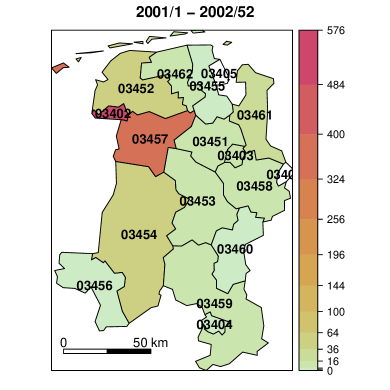
(b)

Figure 13: Measles infections in the Weser-Ems region, 2001–2002.

The overall time-series plot in Figure LABEL:fig:measlesWeserEms1 reveals strong seasonality in the data with slightly different patterns in the two years. The spatial plot in Figure LABEL:fig:measlesWeserEms2 is a tweaked spplot (package sp) with colors from colorspace (Ihaka et al., 2015) using $\sqrt{}$-equidistant cut points handled by package scales (Wickham, 2015). The default plot type is observed   time | unit and shows the individual time series by district (Figure 14):

R> plot(measlesWeserEms, units = which(colSums(observed(measlesWeserEms)) > 0))

Figure 14: Count time series of the 15 affected districts.

The plot excludes the districts 03401 (SK Delmenhorst) and 03405 (SK Wilhelmshaven) without any reported cases. Obviously, the districts have been affected by measles to a very heterogeneous extent during these two years.

An animation of the data can be easily produced as well. We recommend to use converters of the animation package, e.g., to watch the series of plots in a web browser. The following code will generate weekly disease maps during the year 2001 with the respective total number of cases shown in a legend and – if package gridExtra (Auguie, 2015) is available – an evolving time-series plot at the bottom:

R> animation::saveHTML(+    animate(measlesWeserEms, tps = 1:52, total.args = list()),+    title = "Evolution of the measles epidemic in the Weser-Ems region, 2001",+    ani.width = 500, ani.height = 600)

5.3 Modeling and inference

For multivariate surveillance time series of counts such as the measlesWeserEms data, the function hhh4 fits models of the form (10) via (penalized) maximum likelihood. We start by modeling the measles counts in the Weser-Ems region by a slightly simplified version of the original negative binomial model by Held et al. (2005). Instead of district-specific intercepts $\alpha_{i}^{(\nu)}$ in the endemic component, we first assume a common intercept $\alpha^{(\nu)}$ in order to not be forced to exclude the two districts without any reported cases of measles. After the estimation and illustration of this basic model, we will discuss the following sequential extensions: covariates (district-specific vaccination coverage), estimated transmission weights, and random effects to eventually account for unobserved heterogeneity of the districts.

5.3.1 Basic model

Our initial model has the following mean structure:

$$\mu_{it} =e_{i}\,\nu_{t}+\lambda\,Y_{i,t-1}+\phi\sum_{j\neq i}w_{ji}Y_{j,t-1}\>,$$ (14)

$$\log(\nu_{t}) =\alpha^{(\nu)}+\beta_{t}t+\gamma\sin(\omega t)+\delta\cos(\omega t)\>.$$ (15)

To account for temporal variation of disease incidence, the endemic log-linear predictor $\nu_{t}$ incorporates an overall trend and a sinusoidal wave of frequency $\omega=2\pi/52$. As a basic district-specific measure of disease incidence, the population fraction $e_{i}$ is included as a multiplicative offset. The epidemic parameters $\lambda=\exp(\alpha^{(\lambda)})$ and $\phi=\exp(\alpha^{(\phi)})$ are assumed homogeneous across districts and constant over time. Furthermore, we define $w_{ji}=\mathbbm{1}(j\sim i)=\mathbbm{1}(o_{ji}=1)$ for the time being, which means that the epidemic can only arrive from directly adjacent districts. This hhh4 model transforms into the following list of control arguments:

R> measlesModel_basic <- list(+    end = list(f = addSeason2formula(~1 + t, period = measlesWeserEms@freq),+               offset = population(measlesWeserEms)),+    ar = list(f = ~1),+    ne = list(f = ~1, weights = neighbourhood(measlesWeserEms) == 1),+    family = "NegBin1") The formulae of the three predictors $\log\nu_{t}$, $\log\lambda$ and $\log\phi$ are specified as element f of the end, ar, and ne lists, respectively. For the endemic formula we use the convenient function addSeason2formula to generate the sine-cosine terms, and we take the multiplicative offset of population fractions $e_{i}$ from the measlesWeserEms object. The autoregressive part only consists of the intercept $\alpha^{(\lambda)}$, whereas the neighbourhood component specifies the intercept $\alpha^{(\phi)}$ and also the matrix of transmission weights $(w_{ji})$ to use – here a simple indicator of first-order adjacency. The chosen family corresponds to a negative binomial model with a common overdispersion parameter $\psi$ for all districts. Alternatives are "Poisson", "NegBinM" ($\psi_{i}$), or a factor determining which groups of districts share a common overdispersion parameter. Together with the data, the complete list of control arguments is then fed into the hhh4 function to estimate the model, a summary of which is printed below.

R> measlesFit_basic <- hhh4(stsObj = measlesWeserEms, control = measlesModel_basic)R> summary(measlesFit_basic, idx2Exp = TRUE, amplitudeShift = TRUE, maxEV = TRUE)

Call:hhh4(stsObj = measlesWeserEms, control = measlesModel_basic)Coefficients:                      Estimate  Std. Errorexp(ar.1)              0.64540   0.07927exp(ne.1)              0.01581   0.00420exp(end.1)             1.08025   0.27884exp(end.t)             1.00119   0.00426end.A(2 * pi * t/52)   1.16423   0.19212end.s(2 * pi * t/52)  -0.63436   0.13350overdisp               2.01384   0.28544Epidemic dominant eigenvalue:  0.72Log-likelihood:   -972AIC:              1957BIC:              1996Number of units:        17Number of time points:  103 The idx2Exp argument requests the estimates for $\lambda$, $\phi$, $\alpha^{(\nu)}$ and $\exp(\beta_{t})$ instead of their respective internal log-values. For instance, exp(end.t) represents the seasonality-adjusted factor by which the basic endemic incidence increases per week. The amplitudeShift argument transforms the internal coefficients $\gamma$ and $\delta$ of the sine-cosine terms to the amplitude $A$ and phase shift $\varphi$ of the corresponding sinusoidal wave $A\sin(\omega t+\varphi)$ in $\log\nu_{t}$ (Paul et al., 2008). The multiplicative effect of seasonality on $\nu_{t}$ is shown in Figure 15 produced by:

R> plot(measlesFit_basic, type = "season", components = "end", main = "")

Figure 15: Estimated multiplicative effect of seasonality on the endemic mean.

The overdisp parameter and its 95% confidence interval obtained by

R> confint(measlesFit_basic, parm = "overdisp")

         2.5 % 97.5 %overdisp  1.45   2.57 suggest that a negative binomial distribution with overdispersion is more adequate than a Poisson model corresponding to $\psi=0$. We can underpin this finding by an AIC comparison, taking advantage of the convenient update method for hhh4 fits:

R> AIC(measlesFit_basic, update(measlesFit_basic, family = "Poisson"))

                                             df  AICmeaslesFit_basic                              7 1957update(measlesFit_basic, family = "Poisson")  6 2479

The epidemic potential of the process as determined by the parameters $\lambda$ and $\phi$ is best investigated by a combined measure: the dominant eigenvalue (maxEV) of the matrix $\bm{\Lambda}$ which has the entries $(\Lambda)_{ii}=\lambda$ on the diagonal and $(\Lambda)_{ij}=\phi w_{ji}$ for $j\neq i$ (Paul et al., 2008). If the dominant eigenvalue is smaller than unity, it can be interpreted as the epidemic proportion of disease incidence. In the above model, the estimate is 72%. Another way of judging the relative importance of the three model components is to plot the fitted mean components along with the observed counts. Figure 16 shows this for the six districts with more than 20 cases:

R> districts2plot <- which(colSums(observed(measlesWeserEms)) > 20)R> plot(measlesFit_basic, type = "fitted", units = districts2plot, hide0s = TRUE)

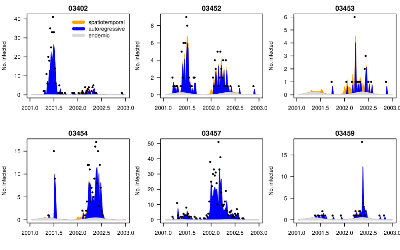
Figure 16: Fitted components in the initial model measlesFit_basic for the six districts with more than 20 cases. Dots are only drawn for positive weekly counts.

The largest portion of the fitted mean indeed results from the within-district autoregressive component with very little contribution of cases from adjacent districts and a rather small endemic incidence.

Other plot types and methods for fitted hhh4 models as listed in Table 8 will be applied in the course of the following model extensions.

Display	Extract	Modify	Other
print	nobs	update	predict
summary	coef		simulate
plot	fixef		pit
	ranef		scores
	vcov		calibrationTest
	confint		all.equal
	coeflist		oneStepAhead
	logLik
	residuals
	terms
	formula

Table 8: Generic and non-generic functions applicable to hhh4 objects.

5.3.2 Covariates

The hhh4 model framework allows for covariate effects on the endemic or epidemic contributions to disease incidence. Covariates may vary over both regions and time and thus obey the same $T\times I$ matrix structure as the observed counts. For infectious disease models, the regional vaccination coverage is an important example of such a covariate, since it reflects the (remaining) susceptible population. In a thorough analysis of measles occurrence in the German federal states, Herzog et al. (2011) found vaccination coverage to be associated with outbreak size. We follow their approach of using the district-specific proportion $1-v_{i}$ of unvaccinated children just starting school as a proxy for the susceptible population. As $v_{i}$ we use the proportion of children vaccinated with at least one dose among the ones presenting their vaccination card at school entry in district $i$ in the year 2004. This time-constant covariate needs to be transformed to the common matrix structure for incorporation in hhh4:

R> Sprop <- matrix(1 - measlesWeserEms@map@data$vacc1.2004,+    nrow = nrow(measlesWeserEms), ncol = ncol(measlesWeserEms), byrow = TRUE)R> summary(Sprop[1, ])

   Min. 1st Qu.  Median    Mean 3rd Qu.    Max. 0.0306  0.0481  0.0581  0.0675  0.0830  0.1400

There are several ways to account for the susceptible proportion in our model, among which the simplest is to update the endemic population offset $e_{i}$ by multiplication with $(1-v_{i})$. Herzog et al. (2011) found that the susceptible proportion is best added as a covariate in the autoregressive component in the form

$$\lambda_{i}\,Y_{i,t-1}=\exp\big{(}\alpha^{(\lambda)}+\beta_{s}\log(1-v_{i})\big{)}\,Y_{i,t-1}=\exp\big{(}\alpha^{(\lambda)}\big{)}\,(1-v_{i})^{\beta_{s}}\,Y_{i,t-1}$$

according to the mass action principle (Keeling and Rohani, 2008). A higher proportion of susceptibles in district $i$ is expected to boost the generation of new infections, i.e., $\beta_{s}>0$. Alternatively, this effect could be assumed as an offset, i.e., $\beta_{s}\equiv 1$. To choose between endemic and/or autoregressive effects, and multiplicative offset vs. covariate modeling, we perform AIC-based model selection. First, we set up a grid of all combinations of envisaged extensions for the endemic and autoregressive components:

R> Soptions <- c("unchanged", "Soffset", "Scovar")R> SmodelGrid <- expand.grid(end = Soptions, ar = Soptions)R> row.names(SmodelGrid) <- do.call("paste", c(SmodelGrid, list(sep = "|"))) Then we update the initial model measlesFit_basic according to each row of SmodelGrid:

R> measlesFits_vacc <- apply(X = SmodelGrid, MARGIN = 1, FUN = function (options) {+    updatecomp <- function (comp, option) switch(option,+      "unchanged" = list(),+      "Soffset" = list(offset = comp$offset * Sprop),+      "Scovar" = list(f = update(comp$f, ~. + log(Sprop))))+    update(measlesFit_basic,+      end = updatecomp(measlesFit_basic$control$end, options[1]),+      ar = updatecomp(measlesFit_basic$control$ar, options[2]),+      data = list(Sprop = Sprop))+    }) The resulting object measlesFits_vacc is a list of 9 hhh4 fits, which are named according to the corresponding Soptions used for the endemic and autoregressive component. We construct a call of the function AIC taking all list elements as arguments:

R> aics_vacc <- do.call(AIC, lapply(names(measlesFits_vacc), as.name),+    envir = as.environment(measlesFits_vacc))R> aics_vacc[order(aics_vacc[, "AIC"]), ]

                    df  AIC`Scovar|unchanged`   8 1917`Scovar|Scovar`      9 1919`Soffset|unchanged`  7 1922`Soffset|Scovar`     8 1924`Scovar|Soffset`     8 1934`Soffset|Soffset`    7 1937unchanged|unchanged  7 1957`unchanged|Scovar`   8 1959`unchanged|Soffset`  7 1967

Hence, AIC increases if the susceptible proportion is only added to the autoregressive component, but we see a remarkable improvement when adding it to the endemic component. The best model is obtained by leaving the autoregressive component unchanged ($\lambda$) and adding the term $\beta_{s}\log(1-v_{i})$ to the endemic predictor in Equation 15.

R> measlesFit_vacc <- measlesFits_vacc[["Scovar|unchanged"]]R> coef(measlesFit_vacc, se = TRUE)["end.log(Sprop)", ]

  Estimate Std. Error     1.718      0.288 The estimated exponent $\hat{\beta}_{s}$ is both clearly positive and different from the offset assumption. In other words, if a district’s fraction of susceptibles is doubled, the endemic measles incidence is estimated to multiply by $2^{\hat{\beta}_{s}}=$ 3.29 (95% CI: 2.23–4.86).

5.3.3 Spatial interaction

Up to now, the model assumed that the epidemic can only arrive from directly adjacent districts because $w_{ji}=\mathbbm{1}(j\sim i)$, and that all districts have the same potential $\phi$ for importing cases from neighbouring regions. Given the ability of humans to travel further and preferrably to metropolitan areas, both assumptions seem overly simplistic. First, to reflect commuter-driven spread in our model, we scale the district’s susceptibility according to its population fraction by multiplying $\phi$ by $e_{i}^{\beta_{pop}}$:

R> measlesFit_nepop <- update(measlesFit_vacc,+    ne = list(f = ~log(pop)), data = list(pop = population(measlesWeserEms))) As in a similar analysis of influenza (Meyer and Held, 2014a), we find strong evidence for such an agglomeration effect: the estimated exponent is $\hat{\beta}_{pop}=$ 2.85 (95% CI: 1.83–3.87) and AIC decreases from 1917 to 1887. Models where attraction to a region scales with population size are called “gravity” models (Xia et al., 2004).

To account for long-range transmission of cases, Meyer and Held (2014a) proposed to estimate the weights $w_{ji}$ as a function of the adjacency order $o_{ji}$ between the districts. For instance, a power-law model assumes the form $w_{ji}=o_{ji}^{-d}$, for $j\neq i$ and $w_{jj}=0$, where the decay parameter $d$ is to be estimated. Normalization to $w_{ji}/\sum_{k}w_{jk}$ is recommended and applied by default when supplying W_powerlaw as weights in the neighbourhood component:

R> measlesFit_powerlaw <- update(measlesFit_nepop,+    ne = list(weights = W_powerlaw(maxlag = 5))) The argument maxlag sets an upper bound for spatial interaction in terms of adjacency order. Here we set no limit since max(neighbourhood(measlesWeserEms)) is 5. The resulting parameter estimate is $\hat{d}=$ 4.10 (95% CI: 2.03–6.17), which represents a strong decay of spatial interaction for higher-order neighbours. As an alternative to the parametric power law, unconstrained weights up to maxlag can be estimated by using W_np instead of W_powerlaw. For instance, W_np(maxlag = 2) corresponds to a second-order model, i.e., $w_{ji}=1\cdot\mathbbm{1}(o_{ji}=1)+e^{\omega_{2}}\cdot\mathbbm{1}(o_{ji}=2)$, which is also row-normalized by default:

R> measlesFit_np2 <- update(measlesFit_nepop,+    ne = list(weights = W_np(maxlag = 2)))

Figure LABEL:fig:measlesFit_neweights2 shows both the power law model $o^{-\hat{d}}$ and the second-order model, where $e^{\hat{\omega}_{2}}=$ 0.09 (95% CI: 0.02–0.39). Alternatively, the plot type = "neweights" for hhh4 fits can produce a stripplot (Sarkar, 2008) of $w_{ji}$ against $o_{ji}$ as shown in Figure LABEL:fig:measlesFit_neweights1 for the power-law model:

R> library("lattice")R> plot(measlesFit_powerlaw, type = "neweights", plotter = stripplot,+    panel = function (...) {panel.stripplot(...); panel.average(...)},+    jitter.data = TRUE, xlab = expression(o[ji]), ylab = expression(w[ji]))

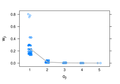
(a)

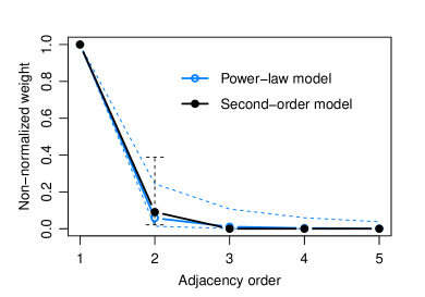
(b)

Figure 17: Estimated weights as a function of adjacency order.

Note that only horizontal jitter is added in this case. Because of normalization, the weight $w_{ji}$ for transmission from district $j$ to district $i$ is determined not only by the districts’ neighbourhood $o_{ji}$ but also by the total amount of neighbourhood of district $j$ in the form of $\sum_{k\neq j}o_{jk}^{-d}$, which causes some variation of the weights for a specific order of adjacency.

An AIC comparison of the different models for the transmission weights yields:

R> AIC(measlesFit_nepop, measlesFit_powerlaw, measlesFit_np2)

                    df  AICmeaslesFit_nepop     9 1887measlesFit_powerlaw 10 1882measlesFit_np2      10 1881 AIC improves when accounting for transmission between higher-order neighbours by a power law or a second-order model. In spite of the latter resulting in a slightly better fit, we will use the power-law model as a basis for further model extensions since the stand-alone second-order effect is not always identifiable in more complex models and is scientifically implausible.

5.3.4 Random effects

Paul and Held (2011) introduced random effects for hhh4 models, which are useful if the districts exhibit heterogeneous incidence levels not explained by observed covariates, and especially if the number of districts is large. For infectious disease surveillance data, a typical example of unobserved heterogeneity is under-reporting (Bernard et al., 2014). Our measles data even contain two districts without any reported cases, while the district with the smallest population (03402, SK Emden) had the second-largest number of cases reported and the highest overall incidence (see Figures LABEL:fig:measlesWeserEms2 and 14). Hence, allowing for district-specific intercepts in the endemic or epidemic components is expected to improve the model fit. For independent random effects $\alpha_{i}^{(\nu)}\stackrel{{\scriptstyle iid}}{{\sim}}\operatorname{N}(\alpha^{(\nu)},\sigma_{\nu}^{2})$, $\alpha_{i}^{(\lambda)}\stackrel{{\scriptstyle iid}}{{\sim}}\operatorname{N}(\alpha^{(\lambda)},\sigma_{\lambda}^{2})$, and $\alpha_{i}^{(\phi)}\stackrel{{\scriptstyle iid}}{{\sim}}\operatorname{N}(\alpha^{(\phi)},\sigma_{\phi}^{2})$ in all three components, we update the corresponding formulae as follows:

R> measlesFit_ri <- update(measlesFit_powerlaw,+    end = list(f = update(formula(measlesFit_powerlaw)$end, ~. + ri() - 1)),+    ar  = list(f = update(formula(measlesFit_powerlaw)$ar,  ~. + ri() - 1)),+    ne  = list(f = update(formula(measlesFit_powerlaw)$ne,  ~. + ri() - 1)))

R> summary(measlesFit_ri, amplitudeShift = TRUE, maxEV = TRUE)

Call:hhh4(stsObj = object$stsObj, control = control)Random effects:            Var   Corrar.ri(iid)  1.076ne.ri(iid)  1.294 0end.ri(iid) 1.312 0    0Fixed effects:                      Estimate  Std. Errorar.ri(iid)            -1.61389   0.38197ne.log(pop)            3.42406   1.07722ne.ri(iid)             6.62429   2.81553end.t                  0.00578   0.00480end.A(2 * pi * t/52)   1.20359   0.20149end.s(2 * pi * t/52)  -0.47916   0.14205end.log(Sprop)         1.79350   0.69159end.ri(iid)            4.42260   1.94605neweights.d            3.60640   0.77602overdisp               0.97723   0.15132Epidemic dominant eigenvalue:  0.84Penalized log-likelihood:  -869Marginal log-likelihood:   -54.2Number of units:        17Number of time points:  103 The summary now contains an extra section with the estimated variance components $\sigma_{\lambda}^{2}$, $\sigma_{\phi}^{2}$, and $\sigma_{\nu}^{2}$ of the random effects. We did not assume correlation between the three intercepts, but this is possible by specifying ri(corr = "all") in the component formulae. The implementation also supports a conditional autoregressive formulation (Besag et al., 1991) for spatially correlated intercepts by using ri(type = "car"). The estimated district-specific intercepts can be extracted by the ranef-method:

R> head(ranef(measlesFit_ri, tomatrix = TRUE), n = 3)

      ar.ri(iid) ne.ri(iid) end.ri(iid)03401      0.000    -0.0567       -1.0003402      1.223     0.0431        1.5303403     -0.827     1.5588       -0.62 They can also be visualized in a map by the plot type = "ri":

R> for (comp in c("ar", "ne", "end")) {+    print(plot(measlesFit_ri, type = "ri", component = comp,+      col.regions = rev(cm.colors(100)), labels = list(cex = 0.6),+      at = seq(-1.6, 1.6, length.out = 15)))+  }

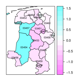
(a)

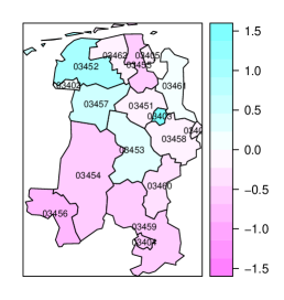
(b)

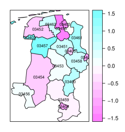
(c)

Figure 18: Maps of the estimated random intercepts.

For the autoregressive component in Figure LABEL:fig:measlesFit_ri_map1, we see a pronounced heterogeneity between the three western districts in blue and the remaining districts. These three districts have been affected by large local outbreaks and are also the ones with the highest overall numbers of cases. In contrast, the city of Oldenburg (03403) is estimated with a relatively low autoregressive factor $\lambda_{i}=\exp(\alpha^{(\lambda)}+\alpha_{i}^{(\lambda)})=0.087$, but it seems to import more cases from other districts than explained by its population (Figure LABEL:fig:measlesFit_ri_map2). In Figure LABEL:fig:measlesFit_ri_map3, the two districts without any reported measles cases (03401 and 03405) appear in dark pink, which means that they exhibit a relatively low endemic incidence after adjusting for the population and susceptible proportion. Such districts could be suspected of a larger amount of under-reporting.

Note that the extra flexiblility of the random effects model comes at a price. First, the estimation runtime increases considerably from 0.1 seconds for the previous power-law model measlesFit_powerlaw to 4 seconds with additional random effects. Furthermore, we no longer obtain AIC values in the model summary, since random effects invalidate simple AIC-based model comparisons (Greven and Kneib, 2010). Of course we can plot the fitted values and visually compare their quality with the initial fit shown in Figure 16:

R> plot(measlesFit_ri, type = "fitted", units = districts2plot, hide0s = TRUE)

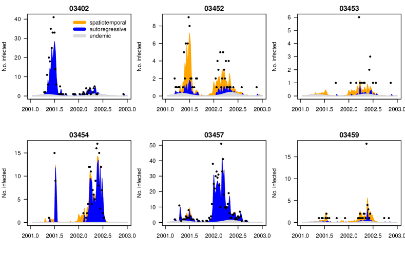
Figure 19: Fitted components in the random effects model measlesFit_ri for the six districts with more than 20 cases. Compare to Figure 16.

For some of these districts, a great amount of cases is now explained via transmission from neighbouring regions while others are mainly influenced by the local autoregression. Note that the estimated decomposition of the mean by district can also be seen from the related plot type = "maps" (not shown). However, for quantitative comparisons of model performance we have to resort to more sophisticated techniques presented in the next section.

5.3.5 Predictive model assessment

Paul and Held (2011) suggest to evaluate one-step-ahead forecasts from competing models by proper scoring rules for count data (Czado et al., 2009). These scores measure the discrepancy between the predictive distribution $P$ from a fitted model and the later observed value $y$. A well-known example is the squared error score (“ses”) $(y-\mu_{P})^{2}$, which is usually averaged over a suitable set of forecasts to obtain the mean squared error. More elaborate scoring rules such as the logarithmic score (“logs”) or the ranked probability score (“rps”) take into account the whole predictive distribution to assess calibration and sharpness simultaneously – see the recent review by Gneiting and Katzfuss (2014). The so-called Dawid-Sebastiani score (“dss”) is another option. Lower scores correspond to better predictions.

In the hhh4 framework, predictive model assessment is made available by the functions oneStepAhead, scores, pit, and calibrationTest. We will use the second quarter of 2002 as the test period, and compare the basic model, the power-law model, and the random effects model. First, we use the "final" fits on the complete time series to compute the predictions, which then simply correspond to the fitted values during the test period:

R> tp <- c(65, 77)R> models2compare <- paste0("measlesFit_", c("basic", "powerlaw", "ri"))R> measlesPreds1 <- lapply(mget(models2compare), oneStepAhead,+    tp = tp, type = "final")

Note that in this case, the log-score for a model’s prediction in district $i$ in week $t$ equals the associated negative log-likelihood contribution. Comparing the mean scores from different models is thus essentially a goodness-of-fit assessment:

R> SCORES <- c("logs", "rps", "dss", "ses")R> measlesScores1 <- lapply(measlesPreds1, scores, which = SCORES, individual = TRUE)R> t(sapply(measlesScores1, colMeans, dims = 2))

                    logs   rps   dss  sesmeaslesFit_basic    1.09 0.736 1.291 5.29measlesFit_powerlaw 1.10 0.731 2.222 5.39measlesFit_ri       1.01 0.638 0.966 4.82

All scoring rules claim that the random effects model gives the best fit during the second quarter of 2002. Now we turn to true one-week-ahead predictions of type = "rolling", which means that we always refit the model up to week $t$ to get predictions for week $t+1$:

R> measlesPreds2 <- lapply(mget(models2compare), oneStepAhead,+    tp = tp, type = "rolling", which.start = "final",+    cores = 2 * (.Platform$OS.type == "unix"))R> measlesScores2 <- lapply(measlesPreds2, scores, which = SCORES, individual = TRUE)R> t(sapply(measlesScores2, colMeans, dims = 2))

                    logs   rps  dss  sesmeaslesFit_basic    1.10 0.748 1.34 5.40measlesFit_powerlaw 1.14 0.765 2.93 5.87measlesFit_ri       1.11 0.763 2.35 7.08

Thus, the most parsimonious initial model measlesFit_basic gives the best one-week-ahead predictions in terms of overall mean scores. Statistical significance of the differences in mean scores can be investigated by a permutationTest for paired data or a paired t-test:

R> set.seed(321)R> sapply(SCORES, function (score) permutationTest(+    measlesScores2$measlesFit_ri[, , score],+    measlesScores2$measlesFit_basic[, , score]))

            logs    rps    dss   sesdiffObs     0.00782 0.0154 1.01  1.68pVal.permut 0.867   0.72   0.518 0.19pVal.t      0.854   0.717  0.374 0.171

Hence, there is no clear evidence for a difference between the basic and the random effects model with regard to predictive performance during the test period. Whether predictions of a particular model are well calibrated can be formally investigated by calibrationTests for count data as recently proposed by (Wei and Held, 2014). For example:

R> calibrationTest(measlesPreds2[["measlesFit_ri"]], which = "rps")

Calibration Test for Count Data (based on RPS)data:  measlesPreds2[["measlesFit_ri"]]z = 0.80671, n = 221, p-value = 0.4198 Thus, there is no evidence of miscalibrated predictions from the random effects model. Czado et al. (2009) describe an alternative informal approach to assess calibration: probability integral transform (PIT) histograms for count data (Figure 20).

R> for (m in models2compare)+    pit(measlesPreds2[[m]], plot = list(ylim = c(0, 1.25), main = m))

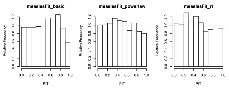
Figure 20: PIT histograms of competing models to check calibration of the one-week-ahead predictions during the second quarter of 2002.

Under the hypothesis of calibration, i.e., $y_{it}\sim P_{it}$ for all predictive distributions $P_{it}$ in the test period, the PIT histogram is uniform. Underdispersed predictions lead to U-shaped histograms, and bias causes skewness. In this aggregate view of the predictions over all districts and weeks of the test period, predictive performance is comparable between the models, and there is no evidence of badly dispersed predictions. However, the right-hand decay in all histograms suggests that all models tend to predict higher counts than observed. This is most likely related to the seasonal shift between the years 2001 and 2002. In 2001, the peak of the epidemic was in the second quarter, while it already occured in the first quarter in 2002 (cp. Figure LABEL:fig:measlesWeserEms1).

5.3.6 Further modeling options

In the previous sections we extended our model for measles in the Weser-Ems region with respect to spatial variation of the counts and their interaction. Temporal variation was only accounted for in the endemic component, which included a long-term trend and a sinusoidal wave on the log-scale. Held and Paul (2012) suggest to also allow seasonal variation of the epidemic force by adding a superposition of $S$ harmonic waves of fundamental frequency $\omega$, $\sum_{s=1}^{S}\left\{\gamma_{s}\sin(s\,\omega t)+\delta_{s}\cos(s\,\omega t)\right\}$, to the log-linear predictors of the autoregressive and/or neighbourhood component – just like for $\log\nu_{t}$ in Equation 15 with $S=1$. However, given only two years of measles surveillance and the apparent shift of seasonality with regard to the start of the outbreak in 2002 compared to 2001, more complex seasonal models are likely to overfit the data. Concerning the coding in R, sine-cosine terms can be added to the epidemic components without difficulties by again using the convenient function addSeason2formula. Updating a previous model for different numbers of harmonics is even simpler, since the update-method has a corresponding argument S. The plots of type = "season" and type = "maxEV" for hhh4 fits can visualize the estimated component seasonality.

All of our models for the measles surveillance data incorporated an epidemic effect of the counts from the local district and its neighbours. Without further notice, we thereby assumed a lag equal to the observation interval of one week. However, the generation time of measles is around 10 days (Anderson and May, 1991), which is why some studies, e.g., Finkenstädt et al. (2002) or Herzog et al. (2011), aggregate their weekly measles surveillance data into biweekly intervals. Fine and Clarkson (1982) used weekly counts in their analysis and report that biweekly aggregation would have little effect on the results. We can also perform such a sensitivity analysis by running the whole code of the current section based on aggregate(measlesWeserEms, nfreq = 26). Doing so, the parameter estimates of the various models retain their order of magnitude and conclusions remain the same. However, with the number of time points halved, the complex random effects model would not always be identifiable when calculating one-week-ahead predictions during the test period.

We have shown several options to account for the spatio-temporal dynamics of infectious disease spread. However, for directly transmitted human diseases, the social phenomenon of “like seeks like” results in contact patterns between subgroups of a population, which extend the pure distance decay of interaction. Especially for school children, social contacts are known to be highly assortative with respect to age (Mossong et al., 2008). A useful epidemic model should therefore be additionally stratified by age group and take the inherent contact structure into account. How this extension can be incorporated in the spatio-temporal endemic-epidemic modeling framework hhh4 is the focus of current research.

5.4 Simulation

Simulation from fitted hhh4 models is enabled by an associated simulate-method. Compared to the point process models of Sections 3 and 4, simulation is less complex since it essentially consists of sequential calls of rnbinom (or rpois). At each time point $t$, the mean $\mu_{it}$ is determined by plugging in the parameter estimates and the counts $Y_{i,t-1}$ simulated at the previous time point. In addition to a model fit, we thus need to specify an initial vector of counts y.start. As an example, we simulate 100 realizations of the evolution of measles during the year 2002 based on the fitted random effects model and the counts of the last week of the year 2001 in the 17 districts:

R> (y.start <- observed(measlesWeserEms)[52, ])

03401 03402 03403 03404 03405 03451 03452 03453 03454 03455 03456 03457 03458 03459    0     0     0     0     0     0     0     0     0     0     0    25     0     003460 03461 03462    0     0     0

R> measlesSim <- simulate(measlesFit_ri,+    nsim = 100, seed = 1, subset = 53:104, y.start = y.start) The simulated counts are returned as a $52\times 17\times 100$ array instead of a list of 100 sts objects. We can, e.g., look at the final size distribution of the simulations:

R> summary(colSums(measlesSim, dims = 2))

   Min. 1st Qu.  Median    Mean 3rd Qu.    Max.    223     326     424     550     582    3970 A few large outbreaks have been simulated, but the mean size is below the observed number of sum(observed(measlesWeserEms)[53:104, ]) $=779$ cases in the year 2002. Using the plot-method associated with such hhh4 simulations, Figure 21 shows the weekly number of observed cases compared to the long-term forecast:

R> plot(measlesSim, "time", ylim = c(0, 100))

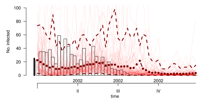
Figure 21: Simulation-based long-term forecast starting from the last week in 2001 (vertical bar on the left), showing the counts aggregated over all districts. The weekly mean of the simulations is represented by dots and the dashed lines correspond to the pointwise 2.5% and 97.5% quantiles. The actually observed counts are shown in the background.

We refer to help("simulate.hhh4") for further examples.

6 Conclusion

In the present work we have introduced the R package surveillance as a comprehensive statistical framework for the analysis of spatio-temporal surveillance data covering individual-level event data as well as aggregated count data time series. The package offers a multitude of methods for visualization, likelihood inference and simulation of endemic-epidemic models. Additional functionality beyond the illustrations in Sections 3 to 5 can be found via help(package = "surveillance"). By the open-source implementation of recently developed statistical methodology in a readily available R package, we support reproducibility of research and hope to serve an increased need in analyzing spatio-temporal epidemic data using statistical models.

Involved R packages and versions

This paper is based on surveillance 1.10-0 (Höhle et al., 2015) in R version 3.2.2 (2015-08-14) using knitr (Xie, 2015) for dynamic report generation. The implementations of the three presented endemic-epidemic modeling frameworks rely on several other R packages. In the following we list all packages involved as first-order dependencies of surveillance with the versions used in this paper: sp 1.2-1 (Pebesma and Bivand, 2005), xtable 1.8-0 (Dahl, 2015), polyCub 0.5-2 (Meyer, 2015), MASS 7.3-44 (Venables and Ripley, 2002), Matrix 1.2-2 (Bates and Maechler, 2015), spatstat 1.43-0 (Baddeley et al., 2015), lattice 0.20-33 (Sarkar, 2008), colorspace 1.2-6 (Ihaka et al., 2015), scales 0.3.0 (Wickham, 2015), quadprog 1.5-5 (Turlach, 2013), memoise 0.2.1 (Wickham, 2014), polyclip 1.3-2 (Johnson, 2015), maptools 0.8-37 (Bivand and Lewin-Koh, 2015) and spdep 0.5-88 (Bivand and Piras, 2015).

R itself, the surveillance package, and all other aforementioned packages are available from the Comprehensive R Archive Network (CRAN) at https://CRAN.R-project.org/. The development of surveillance is hosted at http://surveillance.r-forge.r-project.org/.

References

- Adelfio and Chiodi (2015) Adelfio G, Chiodi M (2015). “FLP Estimation of Semi-parametric Models for Space–time Point Processes and Diagnostic Tools.” Spatial Statistics. ISSN 2211-6753. 10.1016/j.spasta.2015.06.004. In press.
- Anderson and May (1991) Anderson RM, May RM (1991). Infectious Diseases of Humans: Dynamics and Control. Oxford University Press.
- Auguie (2015) Auguie B (2015). \pkggridExtra: Miscellaneous Functions for "Grid" Graphics. \proglangR package version 2.0.0, URL http://CRAN.R-project.org/package=gridExtra.
- Baddeley et al. (2015) Baddeley A, Rubak E, Turner R (2015). Spatial Point Patterns: Methodology and Applications with \proglangR. Chapman and Hall/CRC Press, London. In press, URL http://www.crcpress.com/Spatial-Point-Patterns-Methodology-and-Applications-with-R/Baddeley-Rubak-Turner/9781482210200/.
- Balderama et al. (2012) Balderama E, Schoenberg FP, Murray E, Rundel PW (2012). “Application of Branching Models in the Study of Invasive Species.” Journal of the American Statistical Association, 107(498), 467–476. 10.1080/01621459.2011.641402.
- Bates and Maechler (2015) Bates D, Maechler M (2015). \pkgMatrix: Sparse and Dense Matrix Classes and Methods. \proglangR package version 1.2-2, URL http://CRAN.R-project.org/package=Matrix.
- Bernard et al. (2014) Bernard H, Werber D, Höhle M (2014). “Estimating the Under-Reporting of Norovirus Illness in Germany Utilizing Enhanced Awareness of Diarrhoea During a Large Outbreak of Shiga Toxin-Producing E. Coli O104:H4 in 2011 – A Time Series Analysis.” BMC Infectious Diseases, 14(1), 116. 10.1186/1471-2334-14-116.
- Besag et al. (1991) Besag J, York J, Mollié A (1991). “Bayesian Image-Restoration, with Two Applications in Spatial Statistics.” The Annals of the Institute of Statistical Mathematics, 43(1), 1–20.
- Bivand et al. (2015) Bivand R, Keitt T, Rowlingson B (2015). \pkgrgdal: Bindings for the Geospatial Data Abstraction Library. \proglangR package version 1.1-1, URL http://CRAN.R-project.org/package=rgdal.
- Bivand and Lewin-Koh (2015) Bivand R, Lewin-Koh N (2015). \pkgmaptools: Tools for Reading and Handling Spatial Objects. \proglangR package version 0.8-37, URL http://CRAN.R-project.org/package=maptools.
- Bivand and Piras (2015) Bivand R, Piras G (2015). “Comparing Implementations of Estimation Methods for Spatial Econometrics.” Journal of Statistical Software, 63(18), 1–36. URL http://www.jstatsoft.org/v63/i18/.
- Bivand et al. (2013) Bivand RS, Pebesma E, Gómez-Rubio V (2013). Applied Spatial Data Analysis with \proglangR, volume 10 of Use R! 2nd edition. Springer-Verlag, New York. ISBN 1-4614-7617-8. URL http://www.asdar-book.org.
- Brown (2015) Brown PE (2015). “Model-Based Geostatistics the Easy Way.” Journal of Statistical Software, 63(12), 1–24. ISSN 1548-7660. URL http://www.jstatsoft.org/v63/i12.
- Cori et al. (2013) Cori A, Ferguson NM, Fraser C, Cauchemez S (2013). “A New Framework and Software to Estimate Time-Varying Reproduction Numbers During Epidemics.” American Journal of Epidemiology, 178(9), 1505–1512. 10.1093/aje/kwt133.
- Czado et al. (2009) Czado C, Gneiting T, Held L (2009). “Predictive Model Assessment for Count Data.” Biometrics, 65(4), 1254–1261. 10.1111/j.1541-0420.2009.01191.x.
- Dahl (2015) Dahl DB (2015). \pkgxtable: Export Tables to LaTeX or HTML. \proglangR package version 1.8-0, URL http://CRAN.R-project.org/package=xtable.
- Daley and Gani (1999) Daley DJ, Gani J (1999). Epidemic Modelling: An Introduction, volume 15 of Cambridge Studies in Mathematical Biology. Cambridge University Press. ISBN 0-521-64079-2. 10.1017/CBO9780511608834.
- Daley and Vere-Jones (2003) Daley DJ, Vere-Jones D (2003). An Introduction to the Theory of Point Processes, volume I: Elementary Theory and Methods of Probability and its Applications. 2nd edition. Springer-Verlag, New York. ISBN 0-387-95541-0.
- Diggle (2006) Diggle PJ (2006). “Spatio-Temporal Point Processes, Partial Likelihood, Foot and Mouth Disease.” Statistical Methods in Medical Research, 15(4), 325–336. 10.1191/0962280206sm454oa.
- Douglas and Peucker (1973) Douglas DH, Peucker TK (1973). “Algorithms for the Reduction of the Number of Points Required to Represent a Digitized Line or its Caricature.” Cartographica: The International Journal for Geographic Information and Geovisualization, 10(2), 112–122. 10.3138/FM57-6770-U75U-7727.
- Fahrmeir et al. (2013) Fahrmeir L, Kneib T, Lang S, Marx B (2013). Regression: Models, Methods and Applications. Springer-Verlag. ISBN 3-642-34332-5. 10.1007/978-3-642-34333-9.
- Fine and Clarkson (1982) Fine PEM, Clarkson JA (1982). “Measles in England and Wales—I: An Analysis of Factors Underlying Seasonal Patterns.” International Journal of Epidemiology, 11(1), 5–14. 10.1093/ije/11.1.5.
- Finkenstädt et al. (2002) Finkenstädt BF, Bjørnstad ON, Grenfell BT (2002). “A Stochastic Model for Extinction and Recurrence of Epidemics: Estimation and Inference for Measles Outbreaks.” Biostatistics, 3(4), 493–510. 10.1093/biostatistics/3.4.493.
- Finkenstädt and Grenfell (2000) Finkenstädt BF, Grenfell BT (2000). “Time Series Modelling of Childhood Diseases: A Dynamical Systems Approach.” Journal of the Royal Statistical Society C, 49(2), 187–205. 10.1111/1467-9876.00187.
- Geilhufe et al. (2014) Geilhufe M, Held L, Skrøvseth SO, Simonsen GS, Godtliebsen F (2014). “Power Law Approximations of Movement Network Data for Modeling Infectious Disease Spread.” Biometrical Journal, 56(3), 363–382. 10.1002/bimj.201200262.
- Gneiting and Katzfuss (2014) Gneiting T, Katzfuss M (2014). “Probabilistic Forecasting.” Annual Review of Statistics and Its Application, 1(1), 125–151. 10.1146/annurev-statistics-062713-085831.
- Greven and Kneib (2010) Greven S, Kneib T (2010). “On the Behaviour of Marginal and Conditional AIC in Linear Mixed Models.” Biometrika, 97(4), 773–789. 10.1093/biomet/asq042.
- Groendyke et al. (2012) Groendyke C, Welch D, Hunter DR (2012). “A Network-Based Analysis of the 1861 Hagelloch Measles Data.” Biometrics, 68(3), 755–765. 10.1111/j.1541-0420.2012.01748.x.
- Harrower and Bloch (2006) Harrower M, Bloch M (2006). “Mapshaper.org: A Map Generalization Web Service.” IEEE Computer Graphics and Applications, 26(4), 22–27. 10.1109/MCG.2006.85.
- Held et al. (2006) Held L, Hofmann M, Höhle M, Schmid V (2006). “A Two-Component Model for Counts of Infectious Diseases.” Biostatistics, 7(3), 422–437. 10.1093/biostatistics/kxj016.
- Held et al. (2005) Held L, Höhle M, Hofmann M (2005). “A Statistical Framework for the Analysis of Multivariate Infectious Disease Surveillance Counts.” Statistical Modelling, 5(3), 187–199. 10.1191/1471082X05st098oa.
- Held and Paul (2012) Held L, Paul M (2012). “Modeling Seasonality in Space-Time Infectious Disease Surveillance Data.” Biometrical Journal, 54(6), 824–843. 10.1002/bimj.201200037.
- Herzog et al. (2011) Herzog SA, Paul M, Held L (2011). “Heterogeneity in Vaccination Coverage Explains the Size and Occurrence of Measles Epidemics in German Surveillance Data.” Epidemiology and Infection, 139(04), 505–515. 10.1017/S0950268810001664.
- Hughes and King (2003) Hughes AW, King ML (2003). “Model Selection Using AIC in the Presence of One-Sided Information.” Journal of Statistical Planning and Inference, 115(2), 397–411. 10.1016/S0378-3758(02)00159-3.
- Höhle (2007) Höhle M (2007). “\pkgsurveillance: An \proglangR package for the monitoring of infectious diseases.” Computational Statistics, 22(4), 571–582. 10.1007/s00180-007-0074-8.
- Höhle (2009) Höhle M (2009). “Additive-Multiplicative Regression Models for Spatio-Temporal Epidemics.” Biometrical Journal, 51(6), 961–978. 10.1002/bimj.200900050.
- Höhle (2016) Höhle M (2016). “Infectious Disease Modelling.” In AB Lawson, S Banerjee, RP Haining, MD Ugarte (eds.), Handbook of Spatial Epidemiology, Chapman & Hall/CRC Handbooks of Modern Statistical Methods. Chapman and Hall/CRC. ISBN 1-4822-5301-1. Forthcoming, http://www.math.su.se/~hoehle/pubs/Hoehle_SpaMethInfEpiModelling2015.pdf.
- Höhle and Mazick (2010) Höhle M, Mazick A (2010). “Aberration Detection in \proglangR Illustrated by Danish Mortality Monitoring.” In TA Kass-Hout, X Zhang (eds.), Biosurveillance: Methods and Case Studies, pp. 215–238. Chapman and Hall/CRC.
- Höhle et al. (2015) Höhle M, Meyer S, Paul M (2015). \pkgsurveillance: Temporal and Spatio-Temporal Modeling and Monitoring of Epidemic Phenomena. \proglangR package version 1.10-0, URL http://surveillance.r-forge.r-project.org/.
- Höhle et al. (2009) Höhle M, Paul M, Held L (2009). “Statistical Approaches to the Monitoring and Surveillance of Infectious Diseases for Veterinary Public Health.” Preventive Veterinary Medicine, 91(1), 2–10. 10.1016/j.prevetmed.2009.05.017.
- Ihaka et al. (2015) Ihaka R, Murrell P, Hornik K, Fisher JC, Zeileis A (2015). \pkgcolorspace: Color Space Manipulation. \proglangR package version 1.2-6, URL http://CRAN.R-project.org/package=colorspace.
- Johnson (2015) Johnson A (2015). \pkgpolyclip: Polygon Clipping. \proglangR package version 1.3-2, ported to \proglangR by Adrian Baddeley and Brian Ripley, URL http://CRAN.R-project.org/package=polyclip.
- Johnson (2010) Johnson SD (2010). “A Brief History of the Analysis of Crime Concentration.” European Journal of Applied Mathematics, 21(Special Double Issue 4-5), 349–370. ISSN 1469-4425. 10.1017/S0956792510000082.
- Jombart et al. (2014) Jombart T, Cori A, Didelot X, Cauchemez S, Fraser C, Ferguson N (2014). “Bayesian Reconstruction of Disease Outbreaks by Combining Epidemiologic and Genomic Data.” PLOS Computational Biology, 10(1), e1003457. 10.1371/journal.pcbi.1003457.
- Keeling and Rohani (2008) Keeling MJ, Rohani P (2008). Modeling Infectious Diseases in Humans and Animals. Princeton University Press. ISBN 0-691-11617-2. URL http://www.modelinginfectiousdiseases.org/.
- Kermack and McKendrick (1927) Kermack WO, McKendrick AG (1927). “A Contribution to the Mathematical Theory of Epidemics.” Proceedings of the Royal Society of London A, 115(772), 700–721. 10.1098/rspa.1927.0118.
- Lawson and Leimich (2000) Lawson AB, Leimich P (2000). “Approaches to the Space-Time Modelling of Infectious Disease Behaviour.” IMA Journal of Mathematics Applied in Medicine and Biology, 17(1), 1–13.
- Liboschik et al. (2015) Liboschik T, Fokianos K, Fried R (2015). “\pkgtscount: An R package for analysis of count time series following generalized linear models.” SFB 823 Discussion Paper 6/2015, TU Dortmund. URL http://CRAN.R-project.org/package=tscount.
- Malesios et al. (2014) Malesios C, Demiris N, Kalogeropoulos K, Ntzoufras I (2014). “Bayesian Spatio-Temporal Epidemic Models with Applications to Sheep Pox.” http://arxiv.org/abs/1403.1783.
- Martinussen and Scheike (2002) Martinussen T, Scheike TH (2002). “A Flexible Additive Multiplicative Hazard Model.” Biometrika, 89(2), 283–298. ISSN 0006-3444. 10.1093/biomet/89.2.283.
- Merl et al. (2010) Merl D, Johnson LR, Gramacy RB, Mangel M (2010). “\pkgamei: An R Package for the Adaptive Management of Epidemiological Interventions.” Journal of Statistical Software, 36(6), 1–32. ISSN 1548-7660. URL http://www.jstatsoft.org/v36/i06.
- Meyer (2015) Meyer S (2015). \pkgpolyCub: Cubature over Polygonal Domains. \proglangR package version 0.5-2, URL http://CRAN.R-project.org/package=polyCub.
- Meyer et al. (2012) Meyer S, Elias J, Höhle M (2012). “A Space-Time Conditional Intensity Model for Invasive Meningococcal Disease Occurrence.” Biometrics, 68(2), 607–616. 10.1111/j.1541-0420.2011.01684.x. http://arxiv.org/abs/1508.05740.
- Meyer and Held (2014a) Meyer S, Held L (2014a). “Power-Law Models for Infectious Disease Spread.” The Annals of Applied Statistics, 8(3), 1612–1639. 10.1214/14-AOAS743.
- Meyer and Held (2014b) Meyer S, Held L (2014b). “Supplement B of ‘Power-Law Models for Infectious Disease Spread’.” 10.1214/14-AOAS743SUPPB. http://www.biostat.uzh.ch/research/manuscripts/powerlaw.html.
- Meyer et al. (2015) Meyer S, Warnke I, Rössler W, Held L (2015). “Model-based testing for space-time interaction using point processes: An application to psychiatric hospital admissions in an urban area.” Submitted to Spatial and Spatio-temporal Epidemiology.
- Mohler et al. (2011) Mohler GO, Short MB, Brantingham PJ, Schoenberg FP, Tita GE (2011). “Self-exciting Point Process Modeling of Crime.” Journal of the American Statistical Association, 106(493), 100–108. 10.1198/jasa.2011.ap09546.
- Mossong et al. (2008) Mossong J, Hens N, Jit M, Beutels P, Auranen K, Mikolajczyk R, Massari M, Salmaso S, Tomba GS, Wallinga J, Heijne J, Sadkowska-Todys M, Rosinska M, Edmunds WJ (2008). “Social Contacts and Mixing Patterns Relevant to the Spread of Infectious Diseases.” PLoS Medicine, 5(3), e74. 10.1371/journal.pmed.0050074.
- Neal and Roberts (2004) Neal PJ, Roberts GO (2004). “Statistical Inference and Model Selection for the 1861 Hagelloch Measles Epidemic.” Biostatistics, 5(2), 249–261. 10.1093/biostatistics/5.2.249.
- Obadia et al. (2012) Obadia T, Haneef R, Boelle PY (2012). “The \pkgR0 Package: A Toolbox to Estimate Reproduction Numbers for Epidemic Outbreaks.” BMC Medical Informatics and Decision Making, 12(147). ISSN 1472-6947. 10.1186/1472-6947-12-147.
- Ogata (1988) Ogata Y (1988). “Statistical Models for Earthquake Occurrences and Residual Analysis for Point Processes.” Journal of the American Statistical Association, 83(401), 9–27. URL http://www.jstor.org/stable/2288914.
- Ogata (1999) Ogata Y (1999). “Seismicity Analysis Through Point-process Modeling: A Review.” Pure and Applied Geophysics, 155(2), 471–507. ISSN 0033-4553. 10.1007/s000240050275.
- Paul and Held (2011) Paul M, Held L (2011). “Predictive Assessment of a Non-Linear Random Effects Model for Multivariate Time Series of Infectious Disease Counts.” Statistics in Medicine, 30(10), 1118–1136. 10.1002/sim.4177.
- Paul et al. (2008) Paul M, Held L, Toschke A (2008). “Multivariate Modelling of Infectious Disease Surveillance Data.” Statistics in Medicine, 27(29), 6250–6267. 10.1002/sim.3440.
- Pebesma (2012) Pebesma E (2012). “\pkgspacetime: Spatio-Temporal Data in \proglangR.” Journal of Statistical Software, 51(7), 1–30. URL http://www.jstatsoft.org/v51/i07/.
- Pebesma (2015) Pebesma E (2015). “CRAN Task View: Handling and Analyzing Spatio-Temporal Data.” http://CRAN.R-project.org/web/views/SpatioTemporal.html. Version 2015-09-01.
- Pebesma and Bivand (2005) Pebesma EJ, Bivand RS (2005). “Classes and methods for spatial data in \proglangR.” R News, 5(2), 9–13. URL http://CRAN.R-project.org/doc/Rnews/.
- R Core Team (2015) R Core Team (2015). \proglangR: A Language and Environment for Statistical Computing. \proglangR Foundation for Statistical Computing, Vienna, Austria. URL https://www.R-project.org/.
- Rowlingson and Diggle (2015) Rowlingson B, Diggle P (2015). \pkgsplancs: Spatial and Space-Time Point Pattern Analysis. \proglangR package version 2.01-38, URL http://CRAN.R-project.org/package=splancs.
- Ryan and Ulrich (2014) Ryan JA, Ulrich JM (2014). \pkgxts: eXtensible Time Series. \proglangR package version 0.9-7, URL http://CRAN.R-project.org/package=xts.
- Salmon et al. (2015) Salmon M, Schumacher D, Höhle M (2015). “Monitoring Count Time Series in \proglangR: Aberration Detection in Public Health Surveillance.” Journal of Statistical Software. In press, http://arxiv.org/abs/1411.1292.
- Sarkar (2008) Sarkar D (2008). Lattice: Multivariate Data Visualization with R. Springer, New York. ISBN 978-0-387-75968-5, URL http://lmdvr.r-forge.r-project.org.
- Scheike and Martinussen (2006) Scheike TH, Martinussen T (2006). Dynamic Regression models for survival data. Springer, NY.
- Scheike and Zhang (2011) Scheike TH, Zhang MJ (2011). “Analyzing Competing Risk Data Using the \proglangR \pkgtimereg package.” Journal of Statistical Software, 38(2), 1–15. URL http://www.jstatsoft.org/v38/i02.
- Schrödle et al. (2012) Schrödle B, Held L, Rue H (2012). “Assessing the Impact of a Movement Network on the Spatiotemporal Spread of Infectious Diseases.” Biometrics, 68(3), 736–744. 10.1111/j.1541-0420.2011.01717.x.
- Silvapulle and Sen (2005) Silvapulle MJ, Sen PK (2005). Constrained Statistical Inference: Order, Inequality, and Shape Constraints. Wiley Series in Probability and Statistics. John Wiley & Sons. ISBN 0-471-20827-2.
- Sommariva and Vianello (2007) Sommariva A, Vianello M (2007). “Product Gauss Cubature over Polygons based on Green’s Integration Formula.” Bit Numerical Mathematics, 47(2), 441–453. ISSN 0006-3835. 10.1007/s10543-007-0131-2.
- Stadler and Bonhoeffer (2013) Stadler T, Bonhoeffer S (2013). “Uncovering Epidemiological Dynamics in Heterogeneous Host Populations Using Phylogenetic Methods.” Philosophical Transactions of the Royal Society of London B: Biological Sciences, 368(1614), 20120198. 10.1098/rstb.2012.0198.
- Therneau (2015) Therneau TM (2015). A Package for Survival Analysis in S. Version 2.38, URL http://CRAN.R-project.org/package=survival.
- Turlach (2013) Turlach BA (2013). \pkgquadprog: Functions to solve Quadratic Programming Problems. \proglangR package version 1.5-5, ported to \proglangR by Andreas Weingessel, URL http://CRAN.R-project.org/package=quadprog.
- Utsu et al. (1995) Utsu T, Ogata Y, Matsu’ura RS (1995). “The Centenary of the Omori Formula for a Decay Law of Aftershock Activity.” Journal of Physics of the Earth, 43(1), 1–33. 10.4294/jpe1952.43.1.
- Venables and Ripley (2002) Venables WN, Ripley BD (2002). Modern Applied Statistics with S. Fourth edition. Springer, New York. ISBN 0-387-95457-0, URL http://www.stats.ox.ac.uk/pub/MASS4.
- Vrbik et al. (2012) Vrbik I, Deardon R, Feng Z, Gardner A, Braun J (2012). “Using Individual-level Models for Infectious Disease Spread to Model Spatio-temporal Combustion Dynamics.” Bayesian Analysis, 7(3), 615–638. 10.1214/12-BA721.
- Waller and Gotway (2004) Waller LA, Gotway CA (2004). Applied Spatial Statistics for Public Health Data. Wiley Series in Probability and Statistics. John Wiley & Sons. ISBN 0-471-66267-4. 10.1002/0471662682.
- Wei and Held (2014) Wei W, Held L (2014). “Calibration Tests for Count Data.” TEST, 23(4), 787–805. 10.1007/s11749-014-0380-8.
- Wickham (2014) Wickham H (2014). \pkgmemoise: Memoise functions. \proglangR package version 0.2.1, URL http://CRAN.R-project.org/package=memoise.
- Wickham (2015) Wickham H (2015). \pkgscales: Scale Functions for Visualization. \proglangR package version 0.3.0, URL http://CRAN.R-project.org/package=scales.
- Xia et al. (2004) Xia Y, Bjørnstad ON, Grenfell BT (2004). “Measles Metapopulation Dynamics: A Gravity Model for Epidemiological Coupling and Dynamics.” The American Naturalist, 164(2), 267–281. ISSN 0003-0147. URL http://www.jstor.org/stable/10.1086/422341.
- Xie (2013) Xie Y (2013). “\pkganimation: An \proglangR Package for Creating Animations and Demonstrating Statistical Methods.” Journal of Statistical Software, 53(1), 1–27. URL http://www.jstatsoft.org/v53/i01/.
- Xie (2015) Xie Y (2015). Dynamic Documents with \proglangR and \pkgknitr. The R Series, 2nd edition. Chapman and Hall/CRC, Boca Raton, Florida. ISBN 1-4987-1696-2. URL http://yihui.name/knitr/.