Abstract

We study the problem of estimating a compact set $S\subset\mathbb{R}^{d}$ from a trajectory of a reflected Brownian motion in $S$ with reflections on the boundary of $S$. We establish consistency and rates of convergence for various estimators of $S$ and its boundary. This problem has relevant applications in ecology in estimating the home range of an animal based on tracking data. There are a variety of studies on the habitat of animals that employ the notion of home range. This paper offers theoretical foundations for a new methodology that, under fairly unrestrictive shape assumptions, allows one to find flexible regions close to reality. The theoretical findings are illustrated on simulated and real data examples.

Keywords: set estimation, home-range estimation; reflected Brownian motion.

1 Introduction

Set estimation deals with the problem of approximating, in statistical terms, an unknown compact set $S\subset\mathbb{R}^{d}$. Most of the related literature assumes that the sampling information is given by independent observations whose distribution is closely related to the set $S$. When it comes to set estimation methods, the emphasis in the existing literature is mostly on the geometrical assumptions on $S$ and not on the sampling model. The extent to which a given set estimator efficiently reproduces the unknown set depends heavily on its geometry. Since the early work of Rényi and Sulanke (1963, 1964), significant effort has been made to enlarge the class of sets to estimate, propose efficient estimators, and analyze their asymptotic properties, see Cuevas and Fraiman (2009) for a survey. The best known estimator, introduced by Chevalier (1976), is simply the union of balls centered at the $n$ sample points of radius $\epsilon_{n}$. Devroye and Wise (1980) show that if $\epsilon_{n}\to 0$ and $n\epsilon_{n}^{d}\to\infty$, then the estimate is universally consistent with respect to the measure of the symmetric diference, see (2) for a formal definition. More precisely, they show that the distance in measure converges to 0 in probability for all absolutely continuous distributions supported on $S$. Regarding estimates with geometric shape restrictions, the works of Walther (1997), Rodríguez-Casal (2007) for the class of $r$-convex sets or the more recent work of Cholaquidis et al. (2014) for the class of $\rho$-cone-convex sets show the relevant role of the geometrical assumptions. Recall that a closed convex set can be characterized as the intersection of all closed half spaces containing the set. An $r$-convex set is characterized as the intersection of complements of open balls of radius $r$ that do not intersect the set. This condition implies the outside $r$-rolling condition according to which, informally, at every point of the boundary one can place an open ball included in the complement of the set. In both cases, letting $r\to\infty$, one obtains the convex sets. However, the class of $r$-convex sets is much more flexible, allowing also holes and smooth inlets in the set, see Figure 1. In terms of set estimation, if a set is assumed to be $r$-convex, then it can be efficiently approximated from the $r$-convex hull of a random sample of points taken into it, see Rodríguez-Casal (2007).

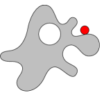
Figure 1: On the left, an example of an $r$-convex set with inlets and holes. The value of $r$ corresponds to the radius of the largest ball that can roll outside the set. The set on the right is neither convex nor $r$-convex for any value of $r$.

The R-package alphahull, described in Pateiro-López and Rodríguez-Casal (2010), provides a practical implementation of the $r$-convex hull estimator for the i.i.d. case in dimension $d=2$. In this work, we are concerned with another aspect of set estimation that has been less studied. We are interested in the problem of estimating an unknown set $S$ from a trajectory of a stochastic process that lives in the set. Up to our knowledge there are no results in the set estimation literature for this framework. We work with the model of reflected Brownian motion. While it is an admittedly simplistic model for many applications, it offers a general, rigorous, and well understood framework. Possible extensions and generalizations are discussed in Section 5 below.

In Section 2, we discuss conditions for the existence of the reflected Brownian motion and its stationary uniform distribution and establish connections between these probabilistic conditions and geometric constraints on its support. In Section 3 we prove consistency of several estimates of $S$ based on a trajectory of a reflected Brownian motion (RBM). We also describe geometric conditions that ensure consistency. In particular, we introduce and study the behaviour of two estimates, the $r$-convex hull of a trajectory and the so-called RBM-sausage. These estimates may be considered as analogues of the $r$-convex hull of a random sample and the Devroye and Wise (1980) estimate in the i.i.d. case, respectively. The study of properties of the Brownian sausage goes back to 1933 (see Kolmogoroff and Leontowitsch (1933)). This estimator is closely related to kernel density estimation (KDE) methods. Indeed, the estimate of Devroye and Wise (1980) is nothing but the set where a kernel density estimator using the uniform kernel is positive. On the other hand, the $r$-convex hull provides a quite flexible family of estimators, with good asymptotic properties in the i.i.d. case. In Section 4 we obtain upper bounds for the rates of convergence.

In Section 5 we generalize the stochastic model generating the observed trajectories. In particular, we consider the general class of reflected diffusions, a class of stochastic processes that include reflected Brownian motion as a special case. This class allows one to deal with processes with non-uniform stationary distribution on the support, an important aspect of some of the applications in home-range estimation. We show that both estimators considered for reflected Brownian motion are well defined and consistent for any kind of reflected diffusion under mild conditions. However, obtaining rates of convergence remain a challenge in the general case. In Section 6 we describe the simulation and real-data studies that illustrate the behavior of the set estimation methods described in the paper. The code used in the paper is available in a new release of the R package alphahull 2.0. Before introducing the formal framework, we discuss the application of the proposed methodology in home-range estimation from animal tracking data, through real data examples.

Home-range estimation is a principal concern in animal ecology. Home range was first defined by Burt (1943) as “the area traversed by the individual in its normal activities of food gathering, mating, and caring for young”. Since this first definition, the concept of home range has evolved, giving rise to a considerable amount of literature on the subject (reviews are given, for instance, by Worton (1987) and Powell (2000)). The home range of an animal is usually estimated from a set of locations collected over a period of time. A first approach was to estimate the animal’s home range by means of the convex hull of the observed location points (Hayne (1949)). This “minimum-convex-polygon” method has well-known shortcomings. A major drawback is that the estimated home range can include areas of land which are never used. This overestimation can be reduced with the use of more flexible estimators such as the $\alpha$-hull, see Burgman and Fox (2003). Other home-range estimation methods describe the animal’s home range by the so-called utilization distribution (density function that describes the probability of finding the animal at a particular location). Since their introduction by Worton (1989) in the context of home-range data, methods based on kernel density estimation have been widely used for estimating the utility distribution. We refer to Seaman and Powell (1996) for an evaluation of the performance of these methods. More recently, Getz and Wilmers (2004) and Getz et al. (2007) proposed the nonparametric kernel method “local convex hull” that estimates the utilization distribution from the union of local nearest-neighbour convex hulls.

These methods of home-range estimation generally treat the recorded locations as independent observations. However, the advances in animal tracking technology (VHF radio transmission, Argos system, GPS, etc.) have allowed one to almost continuously record the movements of animals. In this context, the independence of observations cannot be assumed and new mathematical models are needed. Modelling the movement of an animal in its home range as a continuous stochastic process provides a more realistic framework in which tracking data can be analyzed. Existing stochastic models for describing animal movement can be found in Okubo and Gross (2001), Preisler et al. (2004) and references therein. Other relevant references include Börger et al (2008), Fryxell et al. (2008), Patterson et al (2008) and Tang and Bennet (2010). Some recent results consider more involved statistical problems in the home-range setup which are not covered by our proposal, which only deals with the “densely sampled data”. Fleming et al. (2015) consider the problem of home-range estimation when only a short trajectory is observed and propose a method called AKDE (autocorrelated KDE) that takes into account the autocorrelations to provide a bandwidth (typically much larger) to be used in KDE and predict future animal movement. Buchin et al. (2012) consider the case where the trajectories are only observed at a low sampling rate and analyse animal movement using the Brownian Bridge movement model (BBMM; Horne et al. (2007)), which selects a Brownian Bridge trajectory between each pair of nearest points in time in the low sampling rate original trajectory. On the contrary, the densely sampled data corresponds to a high sampling rate. As mentioned in Kie et al. (2010) “the closer locations are in time, as obtained using GPS technology, the closer locations are in space, and kernel estimators can estimate utilization distribution well without the need for Brownian Bridge”. As we show it in this paper, our proposal works well in this setup. Benhamou (2011) proposes to use movement-based kernel density estimation (MKDE) to estimate the utilization distribution using the circular bivariate Gaussian kernel, where the bandwidth varies for each data-point.

As an alternative approach, mechanistic models (see Moorcroft and Lewis (2006), Potts and Lewis (2014)) incorporate interaction behavior to characterise home ranges. For example, Potts, et al. (2013) (see also Giuggioli et al. (2011)) consider a model where several individuals interact in the home range. “Animals are modeled to move at random but constrained to roam within areas that do not contain scent of cospecifics”. The scent persists for a limited amount of time. Otherwise the individuals perform a nearest neighbor random walk (NNRW) or a ballistic walk (BW).

Because of the fairly unrestrictive nature of the shape assumptions, the methods based on the $r$-convex hull of a trajectory and the RBM-sausage can identify hard boundaries in the home range. Moreover, the estimation is based on a trajectory of a stochastic proccess, more in line with the recent literature on home-range estimation methods. It can be argued that the reflected Brownian motion is a simplified model for animal movement. One of the main limitations of this model is that the stationary distribution is necessarily uniform over the domain, which may not be a realistic assumption for animal movement as it does not allow one to contemplate the notion of “core area” (the area where the animals spend most of the time). A more general related model that incorporates non-uniform stationary distributions is reflected Brownian motion with drift (Kang and Ramanan (2014), Harrison and Williams (1987)). As an alternative, in Section 5 we discuss the general model of reflected diffusions, a class of stochastic processes that include reflected Brownian motion as a special case.

As mentioned before, advances in tracking technology have provided researchers the opportunity to obtain large amount of tracking data from a large variety of species with a high temporal resolution. Movebank is an online database that gives open access to animal movement data collected by researchers. As an illustration, we have considered data from the “Dunn Ranch Bison Tracking Project”. Over the last years, the Nature Conservancy in Missouri (http://www.nature.org/) has been working on the restoration of the Dunn Ranch Prairie, located in northwest Missouri. A herd of bison was introduced onto the ranch in order to restore the prairie ecosystem. The bison roam across a large fenced area. In Figure 2 we show the movements of two bison with $n=9635$ (left), $n=19380$ (right) recorded positions. In red, we represent the boundary of one of the proposed estimators, the $r$-convex hull estimator of the trajectory, for $r=0.005$.

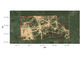
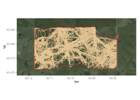
Figure 2: Movements of two bison in the Dunn Ranch Prairie with $n=9635$ (left), $n=19380$ (right) recorded positions. In red, boundary of the $r$-convex hull estimator for $r=0.005$.

For the bison with $n=9635$ recorded positions, we have computed the continuous version of the Devroye-Wise estimator (the reflected Brownian sausage), for different values of the smoothing parameter $\epsilon_{T}$, see Figure 3. A detailed discussion of these estimators is given in the next sections. In Section 6, we analyse the behaviour of the $r$-convex hull estimator with respect to (i) how much the estimated home range differs when we observe the real movement to pass from time 0 to $T$, 0 to $2T$, etc. (short trajectories) and (ii) a variation on the discretization time (low sampling rate).

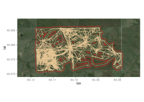
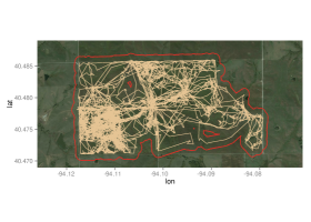
Figure 3: Movements of one bison in the Dunn Ranch Prairie with $n=9635$ recorded positions. In red, boundary of the reflected Brownian sausage $D_{T}$ for $\epsilon_{T}=0.0005$ (left) and $\epsilon_{T}=0.001$ (bottom).

2 Setup

In this section we establish conditions for the existence of the reflected Brownian motion and its stationary uniform distribution, and study the connections between these conditions and some geometric constraints on its support. In particular, we analyze how the regularity required on the support is naturally related to rolling-type properties, which are usual assumptions in set estimation. We first introduce some notation and basic definitions used throughout the manuscript.

Notation and basic definitions.
Given a set $S$, we denote by $\partial S$, $\textnormal{int}(S)$, and $\overline{S}$ the boundary, interior, and closure of $S$, respectively. We denote by $\left\langle\cdot,\cdot\right\rangle$ the usual inner product in $\mathbb{R}^{d}$ and by $\left\|\cdot\right\|$ the Euclidean norm.

Let $\mathcal{B}(x,\epsilon)$ denote the closed ball of radius $\epsilon$ centred at $x$. The open ball is denoted by $\mathring{\mathcal{B}}(x,r)$. Given a bounded set $A\subset\mathbb{R}^{d}$ and $\epsilon>0$, $B(A,\epsilon)$ denotes the parallel set $B(A,\epsilon)=\{x\in\mathbb{R}^{d}:\ d(x,A)\leq\epsilon\}$, where $d(x,A)=\inf\{\|x-a\|:\ a\in A\}$.

Given $x\in\mathbb{R}^{d}$, a unit vector $\xi\in\mathbb{R}^{d}$, and $\rho\in(0,\pi/2]$, $C(x,\xi,\rho)$ denotes the convex cone with vertex $x$, angle $\rho$, and orientation $\xi$, defined by

$$C(x,\xi,\rho)=\big{\{}y\in\mathbb{R}^{d}:\ \left\langle y-x,\xi\right\rangle\geq\left\|y-x\right\|\cos\rho\big{\}}~{}.$$

The closed compact cone of radius $h$ is $C_{h}(x,\xi,\rho)=C(x,\xi,\rho)\cap\mathcal{B}(x,h)$.

The performance of a set estimator is usually evaluated through the Hausdorff distance (1) and the distance in measure (2) given below. The distance in measure takes the mass of the symmetric difference into account while the Hausdorff distance measures the difference of the shapes.

Let $A,C\subset\mathbb{R}^{d}$ be non-empty and compact. The Hausdorff distance between $A$ and $C$ is defined as

$$d_{H}(A,C)=\max\Big{\{}\max_{a\in A}d(a,C),\ \max_{c\in C}d(c,A)\Big{\}}.$$ (1)

If $\mu$ is a Borel measure, the distance in measure between $A$ and $C$ is defined as

$$d_{\mu}(A,C)=\mu(A\triangle C),$$ (2)

where $\triangle$ denotes symmetric difference.

The reflected Brownian motion.

Let $D$ be a domain in $\mathbb{R}^{d}$ (that is, a connected and open set) with closure $\overline{D}$ and boundary $\partial D$. We are concerned with the problem of existence and uniqueness of solution for a reflected stochastic differential equation on the domain $D$. This problem has been discussed by Tanaka (1979) when $D$ is a convex domain and by Lions and Sznitman (1984) and Saisho (1987) when $D$ is a general domain satisfying certain regularity conditions. In particular, Saisho (1987) proved that if $D$ satisfies the uniform exterior sphere condition and the uniform interior cone condition (formalized in Definitions 1 and 2 below), then there exists a unique strong solution of the Skorohod stochastic differential equation

$$X_{t}=X_{0}+B_{t}+\int_{0}^{t}\eta(X_{s})dL_{s},\ t\geq 0,$$ (3)

where $B_{t}$ is a $d$-dimensional Brownian motion, $\eta$ denotes the inward unit vector on the boundary $\partial D$ and $L$ is a continuous nondecreasing process with $L_{0}=0$ and

$$L_{t}=\int_{0}^{t}\mathbb{I}_{\{X_{s}\in\partial D\}}dL_{s}.$$

Roughly speaking, the process behaves in the interior of the set like an ordinary Brownian motion and reflects at the boundary.

Following the notation by Saisho (1987), for $x\in\partial D$, let

$$\mathcal{N}_{x}=\bigcup_{r>0}\mathcal{N}_{x,r},$$

$$\mathcal{N}_{x,r}=\big{\{}\eta\in\mathbb{R}^{d}:\ \left\|\eta\right\|=1,\ \mathring{\mathcal{B}}(x-r\eta,r)\cap D=\emptyset\big{\}}.$$

Definition 1.

The domain $D$ satisfies the uniform exterior sphere condition if there exists a constant $r_{0}>0$ such that, for any $x\in\partial D$,

$$\mathcal{N}_{x}=\mathcal{N}_{x,r_{0}}\neq\emptyset.$$ (4)

For each $x\in\partial D$, the family of sets $\mathcal{N}_{x,r}$ is decreasing with respect to $r$. Condition (4) means that there exists $r_{0}$ such that for all $x\in\partial D$, taking $r\leq r_{0}$ does not add any new direction in $\mathcal{N}_{x,r}$. It is not easy to characterize geometrically this condition. However we prove below that the family of sets that satisfy (4) is between two well-known classes: it is contained in the class of $r_{0}$-convex sets (see Bramson et al. (2012)), and contains the class of sets that satisfies the outside and inside $r_{0}$-rolling condition (stated in the proof of Proposition 3).

Definition 2.

The domain $D$ satisfies the uniform interior cone condition if there exist $\delta>0$ and $\rho\in(0,\pi/2]$ such that for any $x\in\partial D$ there exists a unit vector $l_{x}$ with

$$C(y,l_{x},\rho)\cap\mathring{\mathcal{B}}(x,\delta)\subset\overline{D},\quad\forall y\in\mathring{\mathcal{B}}(x,\delta)\cap\partial D.$$ (5)

In Bramson et al. (2012) it is shown that this condition is equivalent to the domain being Lipschitz (see for instance Definition 9 in Bramson et al. (2012)). From a geometric point of view this condition is related to the cone-convexity property introduced in Cholaquidis et al. (2014): a set $S\subset{\mathbb{R}}^{d}$ is $\rho$-cone-convex, for some $\rho\in(0,\pi/2]$, if there exists $\delta>0$ such that for all $x\in\partial S$ there is an open cone, denoted $\mathring{C}(x,l_{x},\rho)$, such that $\mathring{C}(x,l_{x},\rho)\cap\mathring{\mathcal{B}}(x,\delta)\subset S^{c}$. Condition (5) is stronger than the $\rho$-cone-convexity property in the sense that it requires that the same direction $l_{x}$ works for a neighborhood of $x$.

The trap condition.

Apart from the uniform exterior sphere condition and the uniform interior cone condition, another important notion is that of a non-trap domain. Let $\mathcal{B}\subset D$ and consider the first hitting time of $\mathcal{B}$ by $X$, $T_{\mathcal{B}}=\inf\{t>0:X_{t}\in\mathcal{B}\}$.

Definition 3.

As defined by Burdzy et al. (2006), we say that $D$ is a trap domain for the stochastic process $X_{t}$ if there exists a closed ball $\mathcal{B}\subset D$ with non-zero radius such that

$$\sup_{x\in D}\mathbb{E}^{x}T_{\mathcal{B}}=\infty,$$ (6)

where $\mathbb{E}^{x}$ denotes the expectation of the distribution of $X_{t}$ starting from $x$. Otherwise $D$ is called a non–trap domain.

It is proved in Lemma 3.2 in Burdzy et al. (2006) that if $X_{t}$ is a reflected Brownian motion in

a connected open set $D$ with finite volume and $\mathcal{B}_{1}$ and $\mathcal{B}_{2}$ are closed non–degenerate balls in $D$, then $\sup_{x\in D}\mathbb{E}^{x}T_{\mathcal{B}_{1}}<\infty$ if and only if $\sup_{x\in D}\mathbb{E}^{x}T_{\mathcal{B}_{2}}<\infty$.

The non–trap condition is related to the uniform ergodicity of reflected Brownian motion in $D$. Indeed, this is shown in the following proposition given in Burdzy et al. (2006). Condition (iii) will be used in Section 4 to obtain the rates of convergence of the proposed estimators.

Proposition 1.

(Burdzy et al. (2006), Prop. 1.2) Let $D\subset\mathbb{R}^{d}$ be a connected open set with finite volume, and denote by $\Pi_{D}$ the uniform probability measure in $D$. Let $X_{t}$ be the reflected Brownian motion in $D$. Then the following are equivalent.

• $D$ is a non-trap domain for $X_{t}$;

• $\lim_{t\to\infty}\sup_{x\in D}\|\mathbb{P}^{x}(X_{t}\in\cdot)-\Pi_{D}\|_{TV}=0$;

• There are positive constants $\alpha$ and $\beta$ such that

  $$\sup_{x\in D}\|\mathbb{P}^{x}(X_{t}\in\cdot)-\Pi_{D}\|_{TV}\leq\beta e^{-\alpha t};$$

where $\|\mu\|_{TV}$ stands for the total variation norm of the measure $\mu$.

Consider a non-empty compact set $S\subset\mathbb{R}^{d}$ with connected interior. We show in Proposition 2 below that, if $S=\overline{\textnormal{int}(S)}$ and $\textnormal{int}(S)$ satisfies the uniform interior cone condition, then $\textnormal{int}(S)$ is non-trap. To formalize the argument of the proof, we need the following definitions.

Definition 4.

A bounded domain $D$ satisfies the interior cone condition if there exists $\rho\in(0,\pi/2]$ and $h>0$ such that for all $x\in D$ there exists a unit vector $\xi_{x}$, such that $C_{h}(x,\xi_{x},\rho)\subset D$.

Proposition 2.

Consider a non-empty compact set $S\subset\mathbb{R}^{d}$ with connected interior. Suppose that $S=\overline{\textnormal{int}(S)}$ and $\textnormal{int}(S)$ satisfies the uniform interior cone condition. Then $\textnormal{int}(S)$ is a non-trap domain for the reflected Brownian motion $X_{t}$ in $\textnormal{int}(S)$.

Proof.

First, we prove that, under the stated assumptions, $\textnormal{int}(S)$ satisfies the interior cone condition given in Definition 4. Reasoning by contradiction, if $\textnormal{int}(S)$ does not satisfy the interior cone condition, there exists $x_{n}\in\textnormal{int}(S)$ , and two sequences $\rho_{n}>0$ and $h_{n}>0$ with $\rho_{n},h_{n}\rightarrow 0$ such that

$$\forall\xi\ \text{ with }\left\|\xi\right\|=1,\quad C_{h_{n}}(x_{n},\xi,\rho_{n})\cap\textnormal{int}(S)^{c}\neq\emptyset.$$ (7)

As $S$ is compact, $\{x_{n}\}$ has a subsequential limit $x\in S$. We may assume, (taking a subsequence if necessary) that $x_{n}\rightarrow x$. As $h_{n}\rightarrow 0$ and (7) holds, we have that $x\in\partial S$. Since $\textnormal{int}(S)$ satisfies the uniform interior cone condition, there exist $\delta>0$, $\rho\in(0,\pi/2]$, and a unit vector $l_{x}$ such that (5) holds. Let us take $n$ large enough such that $h_{n}<\delta/4$. Taking $\xi=-l_{x}$ in (7), there exists $y_{n}\in\partial S$ and $y_{n}\in C_{h_{n}}(x_{n},-l_{x},\rho)\cap\textnormal{int}(S)^{c}$. As $h_{n}<\delta/4$ we have that $y_{n}\in\mathcal{B}(x,\delta/2)$. Again by the uniform interior cone condition, we have that $C(y_{n},l_{x},\rho)\cap\mathring{\mathcal{B}}(x,\delta)\subset S$ and $x_{n}\in C(y_{n},l_{x},\rho)$ (see Figure 4). We consider two cases. First, if $x_{n}\in\textnormal{int}(C(y_{n},l_{x},\rho))$, then $C_{h_{n}}(x_{n},l_{x},\rho)\subset\textnormal{int}(C(y_{n},l_{x},\rho))\subset\textnormal{int}(S)$ which contradicts (7). Now, if $x_{n}\in\partial C(y_{n},l_{x},\rho)$ (as in Figure 4) then we can take a unit vector $\nu$ such that $C_{h_{n}}(x_{n},\nu,\rho)\subset C(y_{n},l_{x},\rho)$ and, as $x_{n}\in\textnormal{int}(S)$, $C_{h_{n}}(x_{n},\nu,\rho)\subset\textnormal{int}(S)$ which, again, contradicts (7).

Figure 4: In solid lines the ball $\mathcal{B}(x,\delta/4)$ and the cones $C_{\delta}(x,l_{x},\rho)$, $C_{h_{n}}(x_{n},-l_{x},\rho)$ and $C_{h_{n}}(x_{n},\nu,\rho)$. In dotted lines the cone $C_{\delta}(y_{n},l_{x},\rho)$.

Now, by Lemma 7 in Hajłasz (2001), if a domain satisfies the interior cone condition, then it is a John domain (i.e., there is a constant $C\geq 1$ and a distinguished point $x_{0}\in D$ such that each point $x\in D$ can be joined to $x_{0}$ by a curve $\gamma:[0,1]\rightarrow D$ such that $\gamma(0)=x$, $\gamma(1)=x_{0}$ and $d(\gamma(t),\partial D)\geq C^{-1}\|x-\gamma(t)\|$). Corollary 2.9 and Proposition 1.4 in Burdzy et al. (2006) show that every John domain with finite volume is a non–trap domain. ∎

Rolling-type conditions.  We have shown that if $S\subset\mathbb{R}^{d}$ is a non-empty compact set with with connected interior and $S=\overline{\textnormal{int}(S)}$ such that $\textnormal{int}(S)$ satisfies both the uniform exterior sphere condition and the uniform interior cone condition, then $\textnormal{int}(S)$ is non-trap and there exists a unique strong solution of the Skorohod stochastic differential equation (3). Next we analyze how the required regularity on $\partial S$ is related to three well known rolling-type properties (positive reach, $r$-convexity and outside rolling condition). These rolling-type properties have been used in set estimation as shape restrictions that cover large families of sets (much larger than the family of convex sets). We refer to Cuevas et al. (2012) for more details.

Following the notation in Federer (1959), let $\text{Unp}(S)$ be the set of points $x\in\mathbb{R}^{d}$ having a unique projection on $S$, denoted by $\xi_{S}(x)$. That is, for $x\in\text{Unp}(S)$, $\xi_{S}(x)$ is the unique point that achieves the minimum of $\|x-y\|$ for $y\in S$. We write $\delta_{S}(x)=\inf\{\|x-y\|:y\in S\}$.

Definition 5.

For $x\in S$, let reach$(S,x)=\sup\{r>0:\mathring{\mathcal{B}}(x,r)\subset Unp(S)\big{\}}$. The reach of $S$ is defined by

$$reach(S)=\inf\big{\{}reach(S,x):x\in S\big{\}},$$

and $S$ is said to be of positive reach if $reach(S)>0$.

Definition 6.

A set $S\subset\mathbb{R}^{d}$ is said to be $r$-convex, for $r>0$, if

$$S=C_{r}(S),$$

where

$$C_{r}(S)=\bigcap_{\big{\{}\mathring{\mathcal{B}}(x,r):\ \mathring{\mathcal{B}}(x,r)\cap S=\emptyset\big{\}}}\Big{(}\mathring{\mathcal{B}}(x,r)\Big{)}^{c}$$

is the $r$-convex hull of $S$.

Definition 7.

Let $S\subset\mathbb{R}^{d}$ be a closed set. A ball of radius $r$ is said to roll freely in $S$ if for each boundary point $s\in\partial S$ there exists some $x\in S$ such that $s\in\mathcal{B}(x,r)\subset S$. The set $S$ is said to satisfy the outside $r$-rolling condition if a ball of radius $r$ rolls freely in $\overline{S^{c}}$.

The relationship between positive reach, $r$-convexity, and outside rolling condition is analyzed in Cuevas et al. (2012). It is proved that the class of sets with reach $r$ is included in the class of $r$–convex sets, which is included in the class of sets satisfying the outside $r$–rolling condition. The following result by Bramson et al. (2014) shows the relation of the uniform exterior sphere condition and the uniform interior cone condition to the rolling-type conditions.

Lemma 1.

(Bramson et al. (2014), Lemma A.3) Let $D$ be a bounded domain that satisfies the uniform exterior sphere condition and the uniform interior cone condition. Then $\overline{D}$ has positive reach.

Remark 1.

The relationship between the constant $r_{0}$ of the uniform exterior sphere condition, the angle $\rho$ of the uniform interior cone condition, and the value of $\textnormal{reach}(\overline{D})$ is discussed in Bramson et al. (2014).

Remark 2.

A direct consequence of Lemma 1 and Propositions 1 and 2 in Cuevas et al. (2012) is that if $S\subset\mathbb{R}^{d}$ is a non-empty compact set such that $\textnormal{int}(S)$ satisfies both the uniform exterior sphere condition and the uniform interior cone condition, then $S$ satisfies the outside rolling condition. In fact, we only need to assume that $\textnormal{int}(S)$ satisfies the uniform exterior sphere condition with radius $r_{0}$ to prove that $S$ satisfies the outside $r_{0}$–rolling condition. Note that, if $r_{0}$ is the uniform exterior ball radius, for any $s\in\partial S$, $\mathcal{N}_{s,r_{0}}\neq\emptyset$. Then there exists $\eta:=\eta(s)\in\mathcal{N}_{s,r_{0}}$ such that $\mathring{\mathcal{B}}(s-r_{0}\eta,r_{0})\cap\textnormal{int}(S)=\emptyset$. That is, $s\in\mathcal{B}(s-r_{0}\eta,r_{0})\subset\overline{S^{c}}$ (a ball of radius $r_{0}$ rolls freely in $\overline{S^{c}}$). The converse implication is not true. Consider the set $S=R\setminus\textnormal{int}(A)$, with $R=\left[-1.5,2.5\right]\times\left[-1.5,1.5\right]$ and $A=\mathcal{B}\big{(}(0,0),1\big{)}\cup\mathcal{B}\big{(}(1,0),1\big{)}$, see Figure 5. It is clear that a ball of radius $r_{0}=1$ rolls freely in $\overline{S^{c}}$. We have that $x=(1/2,-\sqrt{3}/2)\in\partial S$. Note that $\mathcal{N}_{x}=\{\eta:\|\eta\|=1,\langle\eta,\xi\rangle\geq\cos(\pi/6)\}$, being $\xi=(0,-1)$, but $\mathcal{N}_{x,1}=\{v_{1},v_{2}\}$ being $v_{1}=(-1/2,-\sqrt{3}/2)$ and $v_{2}=(1/2,-\sqrt{3}/2)$. Therefore, $\textnormal{int}(S)$ does not satisfy the uniform exterior sphere condition with $r_{0}=1$.

Figure 5: In gray, $S=R\setminus\textnormal{int}(A)$, with $R=\left[-1.5,2.5\right]\times\left[-1.5,1.5\right]$ and $A=\mathcal{B}\big{(}(0,0),1\big{)}\cup\mathcal{B}\big{(}(1,0),1\big{)}$. The set $S$ satisfies the outside $r_{0}$–rolling condition for $r_{0}=1$ but $\textnormal{int}(S)$ does not satisfy the uniform exterior sphere condition for $r_{0}=1$.

Proposition 3.

Let $S\subset\mathbb{R}^{d}$ be a non-empty compact set with connected interior satisfying $S=\overline{\textnormal{int}(S)}$. Suppose that for some $r_{0}>0$, a ball of radius $r_{0}>0$ rolls freely in $S$ and $\overline{S^{c}}$. Then the reflected Brownian motion in $\textnormal{int}(S)$ exists and $\textnormal{int}(S)$ is non-trap.

Proof.

By Proposition 2 it is enough to prove that $\textnormal{int}(S)$ satisfies the uniform exterior sphere condition and the uniform interior cone condition. We prove first that the uniform interior cone condition holds. By Theorem 1 of Walther (1999), $\partial S$ is a $(d-1)$-dimensional $C^{1}$ submanifold, and the outward unit vector $\eta(x)$ in a point $x\in\partial S$ is Lipschitz. Then there exists $\delta_{0}>0$ such that for all $x,y\in\partial S$, if $\|x-y\|<\delta_{0}$, the angle between $\eta(x)$ and $\eta(y)$ is smaller than $\pi/6$. As a ball of radius $r_{0}$ rolls freely in $\overline{S^{c}}$ for every point $x\in\partial S$, $C_{r_{0}}(x,-\eta(x),\pi/3)\subset\mathcal{B}(x-\eta(x)r_{0},r_{0})\subset S$. If $y\in\mathring{\mathcal{B}}(x,\delta_{0})\cap\partial S$, $C_{r}(y,-\eta(x),\pi/6)\subset C_{r}(y,-\eta(y),\pi/3)\subset\overline{S^{c}}$. Then, the uniform interior cone condition is satisfied with $\delta=\delta_{0}$ and $\rho=\pi/6$. To prove that the uniform exterior sphere condition is satisfied, observe that by Lemma 2.3 in Pateiro-López and Rodríguez-Casal (2012), for all $x\in\partial S$, $\mathcal{N}_{x,r_{0}}=\eta(x)$ and then $\mathcal{N}_{x,r_{0}}\neq\emptyset$. It remains to prove that $\mathcal{N}_{x}=\mathcal{N}_{x,r_{0}}$. Since $\mathcal{B}(x-r_{0}\eta(x),r_{0})\subset S$ it follows that if for some $r$, $\mathcal{N}_{x,r}\neq\emptyset$ then $\mathcal{N}_{x,r}=\eta(x)$, and then $\mathcal{N}_{x}=\eta(x)$. ∎

3 On the consistency of the estimators

Denote by $W_{T}=\{X_{t}:0\leq t\leq T\}$ the trajectory of the reflected Brownian motion in a domain $S$, up to time $T$. We prove the consistency of several estimates of $S$ based on observing $W_{T}$, both in terms of the Hausdorff distance and distance in measure. Theorem 1 establishes the consistency of any estimate $S_{T}$ containing the trajectory, under the condition that the estimate is contained within $S$ or within $B(S,\varepsilon_{T})$, for $\varepsilon_{T}\rightarrow 0$. We may apply the result to two estimates in particular, the $r$-convex hull of a trajectory, $C_{r}(W_{T})$, and the so-called RBM-sausage $D_{T}=B(W_{T},\epsilon_{T})=\{x\in\mathbb{R}^{d}:\exists t\in[0,T]\ \text{such that}\ \|x-X_{t}\|\leq\epsilon_{T}\}$.

Theorem 1.

Let $S\subset\mathbb{R}^{d}$ be a compact set satisfying $S=\overline{\textnormal{int}(S)}$. Suppose that $\textnormal{int}(S)$ is connected and satisfies conditions (4), (5).

• If $S_{T}$ is any set such that $W_{T}\subset S_{T}\subset S$ a.s., then, with probability one

  $$d_{H}(S_{T},S)\rightarrow 0\quad\text{as }t\rightarrow+\infty.$$

• The same result holds under the weaker condition $W_{T}\subset S_{T}\subset B(S,\varepsilon_{T})$ for some sequence $\varepsilon_{T}\rightarrow 0$.

• In particular, $C_{r}(W_{T})$ and $D_{T}$ are consistent estimates since they satisfy the condition $W_{T}\subset S_{T}\subset B(S,\varepsilon_{T})$.

Proof.

$i)$ As $S_{T}\subset S$, $\forall\varepsilon>0$ we have $S_{T}\subset B(S_{T},\varepsilon)\subset B(S,\varepsilon)$ and we only need to prove that for all $\varepsilon>0$, $S\subset B(S_{T},\varepsilon)$ a.s. for $T$ large enough. Reasoning by contradiction, suppose that there exists $\varepsilon>0$ such that $\forall T>0$ there exists $x_{T}\in S$ but $x_{T}\notin B(S_{T},\varepsilon)$. Then $\mathcal{B}(x_{T},\varepsilon)\cap S_{T}=\emptyset$. As $S$ is compact, there exists $x\in S$ and a sequence $T_{n}\to\infty$ such that $x_{T_{n}}\rightarrow x$ as $n\rightarrow+\infty$. Clearly $\mathring{\mathcal{B}}(x,\varepsilon)\cap S_{T}=\emptyset$ for all $T$. As $S=\overline{\textnormal{int}(S)}$, we can take $z\in\mathcal{B}(x,\varepsilon/2)$ and $0<\delta<\varepsilon/2$ such that $\mathcal{B}(z,\delta)\subset\mathring{\mathcal{B}}(x,\varepsilon)\subset S$. Since $S$ satisfies the non-trap condition (6), with probability one, there exists a time $T_{1}$ such that $X_{T_{1}}\in\mathcal{B}(z,\delta)$, a contradiction. The proof of ii) is similar. ∎

The next theorem establishes the consistency of the $r$-convex hull of the trajectory $W_{t}$ in terms of the distance in measure. In order to use this estimate, one must know a value $r$ for which $S$ is guaranteed to be $r$-convex. Below we discuss how one may avoid this condition by choosing $r$ in a data-dependent manner (see Remark 4).

Theorem 2.

Let $S\subset\mathbb{R}^{d}$ be a compact set satisfying $S=\overline{\textnormal{int}(S)}$. Suppose that $\textnormal{int}(S)$ is connected and satisfies conditions (4), (5). Let $r\in(0,r_{0})$ where $r_{0}$ is the constant given in (4). Then, with probability one,

$$d_{\mu}(C_{r}(W_{T}),S)\rightarrow 0\quad\text{as }T\rightarrow+\infty,$$

where $\mu$ denotes the Lebesgue measure in $\mathbb{R}^{d}$.

Proof.

Observe that $\mu(\partial S)=0$. By Theorem 3 in Cuevas et al. (2012) we have that $d_{H}\big{(}\partial C_{r}(W_{T}),\partial S\big{)}\rightarrow 0$, which implies that $d_{\mu}(C_{r}(W_{T}),S)\rightarrow 0\quad\text{as }T\rightarrow+\infty.$ ∎

In the next result we prove that the surface area of the $r$-convex hull of the trajectory $W_{T}$ is a consistent estimate of the surface area of any $r$-convex set. To make the statement precise, we need the following definitions and a key result by Federer (1959).

Definition 8.

A set $S$ satisfies the property of interior local connectivity if there exists $\alpha_{0}>0$ such that for all $\alpha\leq\alpha_{0}$ and for all $x\in S$, $int(\mathcal{B}(x,\alpha)\cap S)$ is a non-empty connected set.

Definition 9.

The outer Minkowski content of $S\in\mathbb{R}^{d}$ is given by,

$$L_{0}(\partial S)=\lim_{\epsilon\rightarrow 0}\frac{\mu\big{(}B(S,\epsilon)\setminus S\big{)}}{\epsilon},$$

provided that the limit exists and it is finite.

Theorem 3.

(Federer (1959), Th. 5.6) Let $S\subset\mathbb{R}^{d}$ be a compact set with $reach(S)>0$. Let $K$ be a Borel subset of $\mathbb{R}^{d}$. Then there exist unique Radon measures $\Phi_{0}(S,.),\ldots,\Phi_{d}(S,.)$ over $\mathbb{R}^{d}$ such that for $0\leq\epsilon<reach(S)$,

$$\mu(B(S,\epsilon)\cap\{x:\zeta_{S}(x)\in K\})=\sum_{i=0}^{d}\epsilon^{d-i}b_{d-i}\Phi_{i}(S,K),$$

where $b_{0}=1$, $\zeta_{S}(x)$ is the unique projection of $x$ on $S$ and, for $j\geq 1$, $b_{j}$ is the $j$-dimensional measure of a unit ball in $\mathbb{R}^{j}$.

The measures $\Phi_{j}$ are the curvature measures associated with $S$, and in particular, $L_{0}(\partial S)=\Phi_{d-1}(S,\partial S)$.

In what follows we show that the Minkowski content of the $r$-hull of a discretization of the trajectory $W_{T}$ provides a consistent estimate of the surface area of the set $S$ in the two-dimensional case. Note that the result does not imply that $L_{0}(\partial C_{r}(W_{T}))\rightarrow L_{0}(\partial S)$. To prove such a statement one would need that $C_{r}(W_{T})$ satisfies the property of interior local connectivity, which is unclear to us.

Theorem 4.

Let $S\subset\mathbb{R}^{2}$ be a compact set satisfying $S=\overline{\textnormal{int}(S)}$. Suppose that $\textnormal{int}(S)$ is connected and satisfies conditions (4), (5) and the interior local connectivity property. Let $A_{N(T)}\subset W_{T}$ be a sequence of subsets of finite cardinality such that $d_{H}(A_{N(T)},S)\rightarrow 0$ a.s. as $T\rightarrow\infty$. Then

$$L_{0}\big{(}\partial C_{r}(A_{N(T)})\big{)}\rightarrow L_{0}(\partial S)\quad a.s.$$ (8)

Proof.

The proof makes use of the following extension of Lemma 1 in Cuevas et al. (2012)

Lemma 2.

Let $S\subset\mathbb{R}^{2}$ be a compact $r$-convex set satisfying $S=\overline{\textnormal{int}(S)}$ and the property of interior local connectivity. If $A_{N}\subset S$ is a sequence of sets with finite cardinality such that $d_{H}(A_{N},S)\rightarrow 0$, then there exists $r_{0}>0$ such that $\text{reach}\big{(}C_{r}(A_{N})\setminus I(C_{r}(A_{N}))\big{)}>r_{0}$ for all $N$, where $I(C_{r}(A_{N}))$ is the set of isolated points of $C_{r}(A_{N})$ (i.e., $I(C_{r}(A_{N}))=\{x\in C_{r}(A_{N}):B(x,\eta)\cap C_{r}(A_{N})=x\text{ for some }\eta>0\}$).

The proof of Lemma 2 follows the same lines of that of Lemma 1 in Cuevas et al. (2012) with minor changes, so we omit it.

Now, from Lemma 2 we have that both the set $\tilde{S}_{N(T)}=C_{r}\big{(}A_{N(T)}\big{)}\setminus I\big{(}C_{r}(A_{N(T)})\big{)}$ and $S$ have positive reach. Since we also have that $d_{H}(\tilde{S}_{N(T)},S)\rightarrow 0$ a.s., and the assumptions of Theorem 5.9 in Federer (1959) are satisfied (see also Remark 4.14 in that paper) the proof will be complete. Indeed, Theorem 5.9 in Federer (1959) establishes that the curvature measures are continuous with respect to $d_{H}$ (see Remark 5.10 in Federer (1959)). In particular we obtain that $\Phi_{d-1}(\tilde{S}_{N(T)},K)\rightarrow\Phi_{d-1}(S,K)$ for any closed ball $K$ such that $S\subset K$. Using Remark 5.8 in Federer (1959) and $\tilde{S}_{N(T)}\subset S$ we get that $\Phi_{d-1}(\tilde{S}_{N(T)},K)=\Phi_{d-1}(\tilde{S}_{N(T)},K\cap\partial\tilde{S}_{N(T)})=\Phi_{d-1}(\tilde{S}_{N(T)},\partial\tilde{S}_{N(T)})$ and also $\Phi_{d-1}(S,K)=\Phi_{d-1}(S,\partial S)$. The proof of (8) is concluded by noting that $L_{0}(\partial\tilde{S}_{N(T)})=\Phi_{d-1}(\tilde{S}_{N(T)},\partial\tilde{S}_{N(T)})$ and $L_{0}(\partial S)=\Phi_{d-1}(S,\partial S)$. ∎

4 Rates of convergence

In this section we establish upper bounds for the rates of convergence of the set estimates discussed in the previous section (the $r$-convex hull of a trajectory and the RBM-sausage), both for the expected Hausdorff distance and for the expected distance in measure.

Let $S\subset\mathbb{R}^{d}$ be a compact set satisfying $S=\overline{\textnormal{int}(S)}$. Suppose that $D=\textnormal{int}(S)$ is connected. Recall that, if $D$ is non-trap then, by Proposition 1 (iii), there exist constants $\alpha,\beta>0$ such that

$$\sup_{x\in D}\|\mathbb{P}^{x}(X_{t}\in\cdot)-\Pi_{D}\|_{TV}\leq\beta e^{-\alpha t}~{}.$$

These constants and the volume of the domain $S$ play a key role in the following estimate of the rates of convergence of the set estimate.

Theorem 5.

Let $S\subset\mathbb{R}^{d}$ be a compact set such that $S=\overline{\textnormal{int}(S)}$ and $\textnormal{int}(S)$ is a non-trap domain. Let $\{X_{t}:t\geq 0\}$ be a reflected Brownian motion in $S$. Let $S_{T}$ be any measurable set containing the trajectory $W_{T}$ such that $S_{T}\subset S$. Then for all $T>0$ and for $\epsilon<2(2\beta\mu(S)/v_{0})^{1/d}$ (where $v_{0}=\mu(\mathcal{B}(0,1))$ is the volume of the unit ball in $\mathbb{R}^{d}$),

$$\mathbb{P}\{d_{H}(S_{T},S)>\epsilon\}\leq\frac{(\epsilon/4)^{-d}\mu(S)}{v_{0}}\exp\left(-T\frac{(\epsilon/2)^{d}v_{0}\alpha}{2\mu(S)\log\frac{2\beta\mu(S)}{v_{0}(\epsilon/2)^{d}}}\right)~{}.$$

Proof.

Define $\delta=v_{0}(\epsilon/2)^{d}/(2\mu(S))$. Let

$$n=\left\lfloor\frac{T}{\frac{1}{\alpha}\log\frac{\beta}{\delta}}\right\rfloor,$$ (9)

and define $t_{i}=\frac{i}{\alpha}\log\frac{\beta}{\delta}$ for $i=1,\ldots,n$. Note that the condition for $\epsilon$ guarantees that $\beta/\delta>1$. (Roughly speaking, $t_{1},\ldots,t_{n}$ divide the interval $[0,T]$ in $n$ intervals of length $\frac{1}{\alpha}\log\frac{\beta}{\delta}$.)

Denote the $\epsilon$-inner parallel set of $S$ by

$$S^{(\epsilon)}=\{x\in S:\mathcal{B}(x,\epsilon)\subset S\}~{}.$$ (10)

Then

$$\mathbb{P}\{d_{H}(S_{T},S)>\epsilon\} \leq \mathbb{P}\{\exists x\in S^{(\epsilon)}:\forall t\in[0,T]:X_{t}\notin\mathcal{B}(x,\epsilon)\}$$

$$\leq \mathbb{P}\{\exists x\in S^{(\epsilon)}:\forall i\in\{1,2,\ldots,n\}:X_{t_{i}}\notin\mathcal{B}(x,\epsilon)\}~{}.$$

Let $x_{1},\ldots,x_{N}\in S^{(\epsilon)}$ be such that

$$S^{(\epsilon)}\subset\mathcal{B}(x_{1},\epsilon/2)\cup\cdots\cup\mathcal{B}(x_{N},\epsilon/2),$$

and $N$ is the smallest positive integer such that such covering of $S^{(\epsilon)}$ is possible. $N=N(\epsilon/2)$ is called the $\epsilon/2$-covering number of $S^{(\epsilon)}$. It is easy to see (and well known) that $N\leq\mu(S)/\mu(\mathcal{B}(0,\epsilon/4))=(\epsilon/4)^{-d}\mu(S)/v_{0}$.

If for some $x\in S$ we have $X_{t_{i}}\notin\mathcal{B}(x,\epsilon)$ for all $i=1,\ldots,n$, then there exists a $j\in\{1,\ldots,N\}$ such that $X_{t_{i}}\notin\mathcal{B}(x_{j},\epsilon/2)$ for all $i=1,\ldots,n$. Thus, continuing the chain of inequalities above,

$$\mathbb{P}\{d_{H}(S_{T},S)>\epsilon\} \leq \mathbb{P}\{\exists j\in\{1,\ldots,N\}:\forall i\in\{1,2,\ldots,n\}:X_{t_{i}}\notin\mathcal{B}(x_{j},\epsilon/2)\}$$

$$\leq N\sup_{x\in S^{(\epsilon)}}\mathbb{P}\{\forall i\in\{1,2,\ldots,n\}:X_{t_{i}}\notin\mathcal{B}(x,\epsilon/2)\}$$

Next, we estimate the probability on the right-hand side. For all $x\in S$,

$$\mathbb{P}\{\forall i\in\{1,2,\ldots,n\}:X_{t_{i}}\notin\mathcal{B}(x,\epsilon/2)\}$$

$$= \mathbb{P}\{X_{t_{n}}\notin\mathcal{B}(x,\epsilon/2)|\forall i\in\{1,2,\ldots,n-1\}:X_{t_{i}}\notin\mathcal{B}(x,\epsilon/2)\}$$

$$\qquad\times\mathbb{P}\{\forall i\in\{1,2,\ldots,n-1\}:X_{t_{i}}\notin\mathcal{B}(x,\epsilon/2)\}$$

$$= \mathbb{P}\{X_{t_{n}}\notin\mathcal{B}(x,\epsilon/2)|X_{t_{n-1}}\notin\mathcal{B}(x,\epsilon/2)\}\times\mathbb{P}\{\forall i\in\{1,2,\ldots,n-1\}:X_{t_{i}}\notin\mathcal{B}(x,\epsilon/2)\}$$

(since $$X_{t}$$ is a Markov process)

Now, by Proposition 1 (iii),

$$\mathbb{P}\{X_{t_{n}}\notin\mathcal{B}(x,\epsilon/2)|X_{t_{n-1}}\notin\mathcal{B}(x,\epsilon/2)\} \leq 1-\frac{(\epsilon/2)^{d}v_{0}}{\mu(S)}+\beta e^{-\alpha(t_{n}-t_{n-1})}$$

$$= 1-\frac{(\epsilon/2)^{d}v_{0}}{\mu(S)}+\delta$$

$$= 1-\frac{(\epsilon/2)^{d}v_{0}}{2\mu(S)}$$

by the definition of $\delta$. Hence, we have

$$\mathbb{P}\{\forall i\in\{1,2,\ldots,n\}:X_{t_{i}}\notin\mathcal{B}(x,\epsilon/2)\}\leq\left(1-\frac{(\epsilon/2)^{d}v_{0}}{2\mu(S)}\right)\mathbb{P}\{\forall i\in\{1,2,\ldots,n-1\}:X_{t_{i}}\notin\mathcal{B}(x,\epsilon/2)\}$$

and by iterating the argument,

$$\mathbb{P}\{\forall i\in\{1,2,\ldots,n\}:X_{t_{i}}\notin\mathcal{B}(x,\epsilon/2)\}\leq\left(1-\frac{(\epsilon/2)^{d}v_{0}}{2\mu(S)}\right)^{n}\leq\exp\left(-n\frac{(\epsilon/2)^{d}v_{0}}{2\mu(S)}\right)~{}.$$

Summarizing, and substituting the value of $n$ and $\delta$, we have

$$\mathbb{P}\{d_{H}(S_{T},S)>\epsilon\}\leq\frac{(\epsilon/4)^{-d}\mu(S)}{v_{0}}\exp\left(-T\frac{(\epsilon/2)^{d}v_{0}\alpha}{2\mu(S)\log\frac{2\beta\mu(S)}{v_{0}(\epsilon/2)^{d}}}\right)~{}.$$

∎

Theorem 5 implies that, ignoring logarithmic factors, $d_{H}(S_{T},S)$ is roughly of the order of $(T\alpha/\mu(S))^{-1/d}$. More precisely, we have the following:

Corollary 1.

Let $S\subset\mathbb{R}^{d}$ be a compact set such that $S=\overline{\textnormal{int}(S)}$ and $\textnormal{int}(S)$ is a non-trap domain. Let $\{X_{t}:t\geq 0\}$ be a reflected Brownian motion in $S$. Let $S_{T}$ be any measurable set containing the trajectory $W_{T}$ such that $S_{T}\subset S$. Then

$$d_{H}(S_{T},S)=o\Big{(}\Big{(}\frac{\log(T)^{2}}{T}\Big{)}^{1/d}\Big{)}\quad a.s.$$

Proof.

Since $d_{H}(S_{T},S)$ is non-increasing it suffices to prove that

$$d_{H}(S_{n},S)=o\Big{(}\Big{(}\frac{(\log(n))^{2}}{n}\Big{)}^{1/d}\Big{)}\quad a.s.$$

We show that, for all $\epsilon>0$, $\sum_{n=1}^{\infty}\mathbb{P}(a_{n}d_{H}(S_{n},S)>\varepsilon)<\infty$ where $a_{n}=\Big{(}\frac{K\alpha}{3}\frac{n}{(\log(n))^{2}}\Big{)}^{1/d}$ and then apply the Borel-Cantelli lemma. Observe that, if we denote $K=\nu_{0}\epsilon^{d}/(2^{d+1}\mu(S))$, then

$$\mathbb{P}(a_{n}d_{H}(S_{n},S)>\epsilon)\leq \ a_{n}^{d}K^{-1}2^{d-1}\exp\Big{(}-nK\alpha\frac{1}{a_{n}^{d}\log(K^{-1}\beta a_{n}^{d})}\Big{)}$$

$$= \ K^{-1}2^{d-1}\exp\Big{(}\log(a_{n}^{d})-nK\alpha\frac{1}{a_{n}^{d}\log(K^{-1}\beta a_{n}^{d})}\Big{)}.$$

Then $\sum_{n=1}^{\infty}\mathbb{P}(a_{n}d_{H}(S_{n},S)>\varepsilon)<\infty$ follows from the fact that

$$\lim_{n\rightarrow+\infty}\frac{1}{\log(n)}\Big{[}\log(a_{n}^{d})-nK\alpha\frac{1}{a_{n}^{d}\log(K^{-1}\beta a_{n}^{d})}\Big{]}=-2.$$

∎

We may now apply the previous results to analyze the RBM-sausage $D_{T}=B(W_{T},\epsilon_{T})$ for some appropriately chosen decreasing function $\epsilon_{T}$.

Theorem 6.

Let $S\subset\mathbb{R}^{d}$ be a compact set such that $S=\overline{\textnormal{int}(S)}$ and $\textnormal{int}(S)$ is a non-trap domain. Let $\{X_{t}:t\geq 0\}$ be a reflected Brownian motion in $S$. Assume that the surface area $L_{0}(\partial S)$ exists. Let $D_{T}=B(W_{T},\epsilon_{T})$, with $\epsilon_{T}\sim\Big{(}\frac{\log(T)^{2}}{T}\Big{)}^{1/d}$. Then $d_{\mu}(D_{T},S)=\mathcal{O}\Big{(}\Big{(}\frac{\log(T)^{2}}{T}\Big{)}^{1/d}\Big{)}$ a.s.

Proof.

Observe that $\mu(D_{T},S)=\mu(D_{T}\setminus S)+\mu(S\setminus D_{T})$. By the existence of $L_{0}(\partial S)$ we have $\mu(D_{T}\setminus S)=\mathcal{O}(\epsilon_{T})$. Since $W_{T}\subset S$ we may apply Corollary 1 to conclude that $d_{H}(W_{T},S)=o(\epsilon_{T})$ a.s., and then, for $T$ large enough, $S\subset D_{T}$, a.s., so $\mu(S\setminus D_{T})=0$. ∎

Remark 3.

As it is typically the case in non-parametric estimation, the choice of the smoothing parameter is a crucial point. Since in practice the data of the trajectory are always discretized, we suggest two different approaches to select $\varepsilon_{T}$, built from the discretization of the trajectory.

• If we assume that the set $S$ is connected, we may use the analogue of the proposal of Baillo et al (2000) for the i.i.d case. More precisely, the smoothing parameter $\varepsilon_{T}$ is chosen as:

  $$\overline{\epsilon_{T}}=\inf\left\{\epsilon>0:D_{T}\text{ is connected}\right\}.$$

  An easy-to-implement algorithm is also proposed in Baillo et al (2000), reminiscent of the minimal spanning tree.

• For the general case, we suggest the following procedure. After discretization, split the sample at random in two sub-samples $W_{T_{1}}$ and $W_{T_{2}}$ of the same size $n$. Then the smoothing parameter is given by

  $$\overline{\epsilon_{T}}=\inf\left\{\epsilon>0:W_{T_{2}}\subset B(W_{T_{1}},\epsilon)\right\},$$

  which is easy to calculate. Indeed, for each point $W_{i}\in W_{T_{2}}\ \ i=1,\ldots n$, let $d_{i}$ stand for the distance of $W_{i}$ to its nearest neighbor in $W_{T_{1}}$ and let $\mathbf{d}=(d_{1},\ldots,d_{n})$. Then $\overline{\epsilon_{T}}=\max_{i=1,\ldots,n}d_{i}$. A more robust version is to take $\epsilon_{T}$ as the $1-\delta$ quantile of the vector $\mathbf{d}$ for a small value of $\delta$.

Remark 4.

The consistency of the $r$-convex hull estimator $C_{r}(W_{T})$ of the trajectory $W_{T}$ is established in Theorem 2 under the sometimes unrealistic assumption that a lower bound is known for the maximal value of $r_{0}$ under which the set $S$ is $r_{0}$-convex. Here we suggest a way of choosing the parameter $r$ in a data dependent manner. If the set $S$ is $r$–convex for some $r>0$, then it is also $r^{\prime}$–convex for any $0<r^{\prime}<r$ and a sufficiently small value of the parameter will do the job. However, in practice this does not provide a guide to choose the parameter. One may choose $r$ in a data dependent way by selecting $\hat{r}$ satisfying

$$d_{H}\left(C_{\hat{r}}(W_{T}),B(W_{T},\epsilon_{T})\right)\leq\inf_{r>0}d_{H}\left(C_{r}(W_{T}),B(W_{T},\epsilon_{T})\right)+\delta$$

for an arbitrary small $\delta>0$, where $\epsilon_{T}$ is chosen as suggested by Theorem 6. Thus, $\hat{r}$ is a value that makes the $r$–convex hull as close as possible to the RBM–sausage. It is an easy exercise to prove that $C_{\hat{r}}(W_{T})$ is a consistent estimate of $S$ under the conditions of Theorem 2, taking $\delta\rightarrow 0$.

We close this section by establishing rates of convergence of the $r$-convex hull of the trajectory $W_{T}$. For the simplicity of the exposure we concentrate on the $2$-dimensional case. The argument may easily be generalized for $d>2$ to obtain $\mathbb{E}\Big{(}d_{\mu}(S_{T},S)\Big{)}=\mathcal{O}\big{(}\log(T)/T)^{-2/(d+1)}\big{)}.$

Theorem 7.

Let $S\subset\mathbb{R}^{2}$ be a non-empty, connected and compact set such that $S=\overline{\textnormal{int}(S)}$. Suppose that a ball of radius $r$ rolls freely in $S$ and in $\overline{S^{c}}$. Let $\{X_{t}:t\geq 0\}$ be a reflected Brownian motion in $\textnormal{int}(S)$. Let $S_{T}=C_{r}(W_{T})$. Then

$$\mathbb{E}\Big{(}d_{\mu}(S_{T},S)\Big{)}=O((\log(T)/T)^{-2/3})~{},$$

where $\mu$ denotes the Lebesgue measure.

Definition 10.

Let $x\in\mathbb{R}$, $r>0$ and $\mathcal{E}_{x,r}=\big{\{}\mathcal{B}(y,r):y\in\mathcal{B}(x,r)\big{\}}$. Following Pateiro-López and Rodríguez-Casal (2013) the family of subsets $\mathcal{U}_{x,r}$ is said to be unavoidable for $\mathcal{E}_{x,r}$, if, for all $\mathcal{B}(y,r)\in\mathcal{E}_{x,r}$ there exists $U\in\mathcal{U}_{x,r}$ such that $U\subset\mathcal{B}(y,r)$.

Proof.

First observe that, by Proposition 3, the reflected Brownian motion exists and is non-trap. Let $S^{(r/2)}$ be the $r/2$-inner parallel set of $S$ defined in (10). For every $x\in S$ we may take an unavoidable family $\mathcal{U}_{x,r}$ with $6$ elements, such that, for all $U\in\mathcal{U}_{x,r}$, $\mu(U\cap S)\geq L_{1}r^{2}$ if $x\in S^{(r/2)}$, and $\mu(U\cap S)\geq L_{2}r^{1/2}d(x,\partial S)^{3/2}$ if $x\in S\setminus S^{(r/2)}$ where $L_{1}$ and $L_{2}$ are positive constants (see Propositions 1 and 2 in Pateiro-López and Rodríguez-Casal (2013)). Then

$$\mathbb{E}\big{(}d_{\mu}(S,S_{T})\big{)} \leq\int_{S}\sum_{U\in\mathcal{U}_{x,r}}\mathbb{P}\big{(}U\cap W_{T}=\emptyset\big{)}dx$$

$$=\int_{S_{1}}\sum_{U\in\mathcal{U}_{x,r}}\mathbb{P}\big{(}U\cap W_{T}=\emptyset\big{)}dx+\int_{S_{2}}\sum_{U\in\mathcal{U}_{x,r}}\mathbb{P}\big{(}U\cap W_{T}=\emptyset\big{)}dx.$$ (12)

Where $S_{1}=S\setminus S^{(r/2)}$ and $S_{2}=S^{(r/2)}$. First we bound the second term in (4). Define $\delta=L_{2}r^{2}/2$, $n$ as in (9). Since a $r$-convex set is also $r^{\prime}$-convex, with $r^{\prime}<r$, we can assume without loss of generality that $r/2<1$ and $\beta/\delta>1$. Define $t_{i}=\frac{i}{\alpha}\log\frac{\beta}{\delta}$ for $i=1,\ldots,n$. For all $U\in\mathcal{U}_{x,r}$,

$$\mathbb{P}\{U\cap W_{T}=\emptyset\}\leq\mathbb{P}\{\forall i\in\{1,2,\ldots,n\}:X_{t_{i}}\notin U\}.$$

Now, if we proceed as in (4),

$$\mathbb{P}\{\forall i\in\{1,2,\ldots,n\}:X_{t_{i}}\notin U\}=\mathbb{P}\{X_{t_{n}}\notin U|X_{t_{n-1}}\notin U\}\mathbb{P}\{\forall i\in\{1,2,\ldots,n-1\}:X_{t_{i}}\notin U\},$$

and by Proposition 1 (iii),

$$\mathbb{P}\{X_{t_{n}}\notin U|X_{t_{n-1}}\notin U\} \leq 1-L_{2}r^{2}+\beta e^{-\alpha(t_{n}-t_{n-1})}$$

$$= 1-L_{2}r^{2}+\delta$$

$$= 1-\frac{L_{2}r^{2}}{2},$$

by the definition of $\delta$. Hence, we have

$$\mathbb{P}\{\forall i\in\{1,2,\ldots,n\}:X_{t_{i}}\notin U\}\leq\left(1-\frac{L_{1}r^{2}}{2}\right)^{n}\leq\exp\left(-n\frac{L_{1}r^{2}}{2}\right)~{}.$$

Then the second term is $\mathcal{O}(e^{-k_{1}T})$ for some constant $k_{1}>0$. To deal with the first term, we proceed the same way as before. If we take $\delta=\frac{L_{2}r^{1/2}d(x,\partial S)^{3/2}}{2}$ (observe that $\beta/\delta>1$), we have that

$$\mathbb{P}\{\forall i\in\{1,2,\ldots,n\}:X_{t_{i}}\notin U\}\leq \left(1-\frac{L_{2}r^{1/2}d(x,\partial S)^{3/2}}{2}\right)^{n}$$

$$\leq \exp\left(-n\frac{L_{2}r^{1/2}d(x,\partial S)^{3/2}}{2}\right)$$

$$\leq \exp\left(-\frac{T}{\frac{1}{\alpha}\log\big{(}\frac{2\beta}{L_{2}r^{1/2}d(x,\partial S)^{3/2}}\big{)}}\frac{L_{2}r^{1/2}d(x,\partial S)^{3/2}}{2}\right)~{}.$$

Then,

$$\int_{S_{1}}\sum_{U\in\mathcal{U}_{x,r}}\mathbb{P}\big{(}U\cap W_{T}=\emptyset\big{)}dx\leq \ 6\int_{S_{1}}\exp\left(-\frac{T}{\frac{1}{\alpha}\log\big{(}\frac{2\beta}{L_{2}r^{1/2}d(x,\partial S)^{3/2}}\big{)}}\frac{L_{2}r^{1/2}d(x,\partial S)^{3/2}}{2}\right)dx~{}.$$

Let $F(u)=\mu\{x\in S:d(x,\partial S)\leq u\}$ be the distribution of the distance to the boundary $\partial S$ with respect to the Lebesgue measure. Since the set $\overline{S^{c}}$ has positive reach, $F$ is polynomial in $u$) (see Pateiro-López and Rodríguez-Casal (2012)) and $m=\max_{u\in[0,r/2]}F^{\prime}(u)<\infty$. Then, if $u=d(x,\partial S)$,

$$\int_{S_{1}}\sum_{U\in\mathcal{U}_{x,r}}\mathbb{P}\big{(}U\cap W_{T}=\emptyset\big{)}dx\leq \ 6m\int_{0}^{r/2}\exp\left(-\frac{T}{\frac{1}{\alpha}\log\big{(}\frac{2\beta}{L_{2}r^{1/2}u^{3/2}}\big{)}}\frac{L_{2}r^{1/2}u^{3/2}}{2}\right)du~{}.$$ (13)

Now let $z=\alpha TL_{2}r^{1/2}u^{3/2}/2\doteq c_{1}Tu^{3/2}$. Then

$$\int_{0}^{r/2}\exp\left(-\frac{T}{\frac{1}{\alpha}\log\big{(}\frac{2\beta}{L_{2}r^{1/2}u^{3/2}}\big{)}}\frac{L_{2}r^{1/2}u^{3/2}}{2}\right)du=\\ \frac{2}{3}(Tc_{1})^{-2/3}\int_{0}^{c_{1}T(r/2)^{3/2}}z^{-1/3}\exp\left(-\frac{z}{\log\big{(}\frac{\beta\alpha T}{z}\big{)}}\right)dz.\\$$

Since $r^{3/2}<1$,

$$\frac{1}{T^{\frac{2}{3}}}\int_{0}^{c_{1}T(\frac{r}{2})^{\frac{3}{2}}}\frac{1}{z^{\frac{1}{3}}}\exp\left(-\frac{z}{\log\big{(}\frac{\beta\alpha T}{z}\big{)}}\right)dz\leq\frac{1}{T^{\frac{2}{3}}}\int_{0}^{c_{1}T}\frac{1}{z^{\frac{1}{3}}}\exp\left(-\frac{z}{\log\big{(}\frac{\beta\alpha T}{z}\big{)}}\right)dz.$$ (14)

Taking $T$ large enough such that $c_{1}T>\alpha\beta$, we can majorize the right hand side of (14) by

$$\frac{1}{T^{\frac{2}{3}}}\int_{0}^{\alpha\beta}\frac{1}{z^{\frac{1}{3}}}\exp\left(-\frac{z}{\log\big{(}\frac{\beta\alpha T}{z}\big{)}}\right)dz+\frac{1}{T^{\frac{2}{3}}}\int_{\alpha\beta}^{c_{1}T}\frac{1}{z^{\frac{1}{3}}}\exp\left(-\frac{z}{\log(T)}\right)dz~{}.$$

Finally, taking $s=\frac{z}{\log(T)}$,

$$\int_{\alpha\beta}^{c_{1}T}\frac{1}{z^{\frac{1}{3}}}\exp\left(-\frac{z}{\log(T)}\right)dz= \log(T)^{2/3}\int_{\alpha\beta/\log(T)}^{c_{1}T/\log(T)}\frac{1}{s^{\frac{1}{3}}}\exp(-s)ds$$

$$\leq \log(T)^{2/3}\int_{0}^{+\infty}\frac{1}{s^{\frac{1}{3}}}\exp(-s)ds=K(\log(T))^{2/3}.$$

∎

5 Reflected diffusions

As mentioned in the introduction, even though the reflected Brownian motion is a natural model, it may be too simplistic for some applications. In particular, the fact that its stationary distribution is uniform on the domain fails to capture some important aspects of animal movement. In order to address this problem, we suggest the more general, albeit less understood, model of reflected diffusions.

A reflected diffusion in a connected and open domain $D\subset\mathbb{R}^{d}$ corresponds to the solution of the stochastic equation

$$X_{t}=X_{0}+U_{t}+\int_{0}^{t}\eta(X_{s})dL_{s},$$ (15)

where

$$U_{t}=\int_{0}^{t}\sigma(X_{s})dB_{s}+\int_{0}^{t}b(X_{s})ds,$$

and $B_{t}$ is a $d$-dimensional Brownian motion, $\eta$ denotes the inward unit vector on the boundary $\partial D$, $L$ is a continuous nondecreasing process with $L_{0}=0$, and

$$L_{t}=\int_{0}^{t}\mathbb{I}_{\{X_{s}\in\partial D\}}dL_{s}.$$

Saisho (1987) proved that under the geometric conditions (4) and (5) there exists a unique strong solution to (15) whenever $\sigma$ and $b$ are Lipschitz functions.

By taking $\sigma=1$ and $b=0$, one recovers reflected Brownian motions. By other choices of $\sigma$ and $b$ one obtains a rich class of stochastic processes with possibly non-uniform stationary distribution. A simple special case is the reflected Brownian motion with constant drift $\mu$, that corresponds to $U_{t}=B_{t}+t\mu$ in (15). Harrison and Williams (1987) proved that in this case, the stationary distribution has the form $C(\mu)\exp(\langle\gamma(\mu),x\rangle)$ for some $C(\mu)>0$ and $\gamma(\mu)\in\mathbb{R}^{d}$.

Assuming that the domain $D$ is non-trap for the reflected diffusion $X_{t}$, one may generalize Theorem 1. Indeed, by observing that the proof of the theorem relies on the non-trap condition, we have that if $S$ is a compact set satisfying $S=\overline{S}$ and $int(S)$ is connected, for any reflected diffusion in $int(S)$ for which $int(S)$ is non-trap,

• $d_{H}(S_{T},S)\rightarrow 0$ as $T\rightarrow+\infty$, under condition $W_{T}\subset S_{T}\subset B(S,\varepsilon_{T})$ for some sequence $\varepsilon_{T}\rightarrow 0$ and any $S_{T}$ which contains the trajectory $W_{T}=\{X_{t}:0\leq t\leq T\}$.

• In particular, $C_{r}(W_{T})$ and $D_{T}$ are consistent estimates since they satisfy the condition $W_{T}\subset S_{T}\subset B(S,\varepsilon_{T})$.

On the other hand, the non-trap condition is close to be necessary for consistency of $D_{T}$. In fact, is necessary for the complete convergence with respect to the Hausdorff distance. Indeed, if $int(S)$ is a trap domain, there exists a closed ball $B$ with radius $\delta>0$ and a sequence $x_{n}\in int(S)$ such that $\mathbb{E}(T^{x_{n}}_{B})\rightarrow+\infty$. Let $\epsilon<\delta/4$. If $d_{H}(S_{T},S)$ converges to $0$ completely, then

$$\sum_{n=1}^{\infty}P(d_{H}(S_{n},S)>\epsilon)=:A<\infty.$$ (16)

By choosing $x_{0}\in int(S)$ such that $\mathbb{E}(T^{x_{0}}_{B})>A+1$, we have $\sum_{n=1}^{\infty}P(T_{B}^{x_{0}})>A$. On the other hand, for all $n$ we have $\{\omega:T_{B}^{x_{0}}>0\}\subset\{\omega:d_{H}(D_{n},S)>\epsilon\},$ contradicting (16).

Understanding the geometric conditions for the domain that imply the non-trap property for general reflected diffusions remains an interesting research problem.

Also, to obtain rates of convergence for general reflected diffusions remains an open problem. In particular, one needs to extend Proposition 1 in Burdzy et al. (2006) to the case of general diffusions with non-uniform stationary distribution.

6 Some comments on the implementation of the estimators

In practice, given a trajectory $\{X_{t}:0\leq t\leq T\}$ in the plane, we can approximate the $r$-convex hull of the trajectory and the RBM-sausage estimator, by adapting the implementation in the i.i.d. case. The computation of the $r$-convex hull estimator is based on the algorithms presented by Edelsbrunner et al. (1983). The details of its implementation in R (R Core Team (2014)) can be found in Pateiro-López and Rodríguez-Casal (2010). Regarding the RBM-sausage estimator, the implementation is based on the computation of intersections of pairs of balls of radius $\epsilon_{T}$. We refer to Edelsbrunner (1995) for efficient algorithms on the structure of a union of balls. The code for the computation of the $r$-convex hull of the trajectory and the RBM-sausage estimator is available in a new release of the R package alphahull 2.0 that includes specific functions for these methods.

Next, we present an illustration of the estimation of a non-convex compact set $S\subset\mathbb{R}^{2}$ from a simulated trajectory of a planar reflected Brownian motion. An application to real data sets in the context of home-range estimation is discussed in Section 1.

Let $C$ be the region delimited by the so-called crooked egg curve. The polar equation of the crooked egg curve is

$$r=\sin^{3}(\theta)+\cos^{3}(\theta).$$

Points $(x,y)$ in the curve satisfy $(x^{2}+y^{2})^{2}-(x^{3}+y^{3})=0$. Let us consider the set $S=C\setminus\mathring{\mathcal{B}}$ with $\mathring{\mathcal{B}}=\mathring{\mathcal{B}}\big{(}(0.05,0.6),0.15\big{)}$. In Figure 6 we have simulated trajectories of a reflected Brownian motion on $S$. The reflection is pushed in the direction of the inward unit normal vector on the boundary. We represent in red, the boundary of the RBM-sausage $D_{T}$. We analyse the behaviour of $D_{T}$ with respect to how much the estimation differs when the algorithm is applied to a path from time 0 to $T$, or to the same path from time 0 to $2T$, etc. (short trajectories). The behaviour of the estimator is similar to that of the BBMM represented in green. The results based on the BBMM are provided in the R package BBMM, see Nielson et al. (2013). Since these are simulated data, the choice of the location error is based on visual exploration of the result. We assume that the trajectories are observed at a high sampling rate and the parameter corresponding to the time between successive observations is set small.

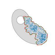
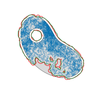
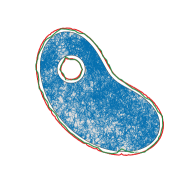
Figure 6: In gray, support limited by a crooked egg curve and a circumference. In blue, path of a simulated reflected Brownian motion. From left to right, size $N=1000$, $N=5000$ and $N=10000$ (with step $h=0.001$). In red, boundary of the RBM-sausage $D_{T}$ for $\epsilon_{T}=0.04$. In green, home-range estimation based on the BBMM (99% utilization distribution estimated).

In Figure 7 we show the $r$-convex hull estimator and analyse its behaviour for lower sampling rates. We start with a simulated reflected Brownian motion with size $N=10000$ and step $h=0.001$ (left) and then select $N=2000$ (middle) and $N=500$ (right) equally spaced in time points. We also show the results based on the BBMM, choosing increasing values of the parameter corresponding to the time between successive observations. As expected, see Horne et al. (2007), the BBMM identifies the movement path with progressively less confidence as the time interval increases.

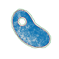
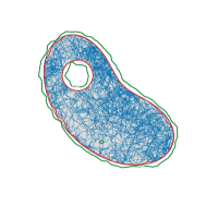
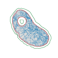
Figure 7: In blue, path of a simulated reflected Brownian motion with size $N=10000$ and step $h=0.001$. In red, boundary of the $r$-convex hull estimator for $r=0.1$ for the original path (left), $N=2000$ (middle) and $N=500$ (right) equally spaced in time points. In green, home-range estimation based on the BBMM (99% utilization distribution estimated).

7 Concluding remarks

We present a new approach to estimate the support of the stationary distribution of a reflected diffusion based on a single trajectory. We consider two estimators: the $r$-convex hull of the trajectory and the Devroye-Wise estimate. Under the non-trap assumption both estimates are consistent with respect to the Hausdorff distance, as well as the distance in measure. These conditions are necessary in order to obtain complete consistency. We also provide algorithms for efficient computation of the estimates.

Our main application is the home-range estimation problem. We illustrate the behaviour of our proposal through two real data examples as well as simulated data. We also compare with the BBMM method in two different setups: short trajectories and low sampling rates. The results are encouraging.

We study in detail the case of the reflected Brownian motion and we obtain rates of convergence with respect to the Hausdorff metric, the distance in measure, and the $L^{1}$ distance.

References

- Baillo et al (2000) Bailo, A., Cuevas. A, and Justel, A.(2000) Set estimation and nonparametric detection. The Canadian Journal of Statistics 28(4), 765–782.
- Benhamou (2011) Benhamou, S.(2011) Dynamic Approach to Space and Habitat Use Based on Biased Random Bridges. PLoS One 6(1).
- Börger et al (2008) Börger, L., Benjamin D. and Fryxell, J.M.(2008) Are there general mechanisms of animal home range behavior? A review and prospects for future research. Ecology Letters. 11, 637–650.
- Bramson et al. (2014) Bramson, M., Burdzy, K. and Kendall, W.(2014) Rubber bands, pursuit games and shy couplings Proc. London Math. Soc. doi: 10.1112/plms/pdt067
- Bramson et al. (2012) Bramson, M., Burdzy, K. and Kendall, W.(2012) Shy Couplings, CAT(0) Spaces, and the Lion and Man. The Annals of Probability 41(2), 744–784
- Buchin et al. (2012) Buchin, K., Arseneau, T., Sijben, S. and Willems, E. Detecting movement patterns using Brownian Bridges. Proceedings of the 20th International Conference on Advances in Geographic Information Systems pp. 119-128.
- Burdzy et al. (2004) Burdzy, K., Chen, Z-Q. and Sylvester, J. (2004). The heat equation and reflected Brownian motion in time-dependent domains. The Annals of Probability. 32, 775–804.
- Burdzy et al. (2006) Burdzy, K., Chen, Z-Q. and Marshall, D. E. (2006). Traps for reflected Brownian motion. Mathematische Zeitschrift 252, 103–132.
- Burgman and Fox (2003) Burgman, M. A. and Fox, J. C. (2003). Bias in species range estimates from minimum convex polygons: implications for conservation and options for improved planning. Animal Conservation 6, 19–28.
- Burt (1943) Burt, W. H.(1943). Territoriality and Home Range Concepts as Applied to Mammals. Journal of Mammalogy 24, 346–352.
- Chevalier (1976) Chevalier, J. (1976) Estimation du support et du contour de support d’une loi de probabilité. Ann. Inst. H. Poincaré B , 339–364.
- Cholaquidis et al. (2014) Cholaquidis, A., Cuevas, A., and Fraiman, R (2014) On Poincaré cone property. Ann. Statist. 42, 255–284.
- Cuevas and Fraiman (2009) Cuevas, A. and Fraiman, R. (2009). Set estimation. In New Perspectives on Stochastic Geometry, eds W.S. Kendall and I. Molchanov. Oxford University Press, pp. 366–389.
- Cuevas et al. (2012) Cuevas, A., Fraiman, R. and Pateiro-López, B. (2012) On statistical properties of sets fullfilling rolling-type conditions. Adv. in Appl. Probab. 44, 311–239.
- Devroye and Wise (1980) Devroye, L. and Wise, G. (1980) Detection of abnormal behaviour via nonparametric estimation of the support. SIAM J. Appl. Math. 3, 480–488.
- Dunn and Gipson (1977) Dunn, J. E. and Gipson, P. S. (1977) Analysis of Radio Telemetry Data in Studies of Home Range. Biometrics 33, 85–101.
- Edelsbrunner (1995) Edelsbrunner, H. (1995). The Union of Balls and Its Dual Shape. Discrete & Computational Geometry, 13 415–440.
- Edelsbrunner et al. (1983) Edelsbrunner, H., Kirkpatrick D.G. and Seidel, R. (1983) On the shape of a set of points in the plane. IEEE Trans. Inform. Theory 29, 551–559.
- Federer (1959) Federer, H. (1959) Curvature measures. Trans. Amer. Math. Soc. 93, 418–491.
- Fleming et al. (2015) Fleming, C.H., Muller, T., Olson, K.A., Leimgruber, P. and Calabrese, J.M. (2015) Rigorous home range estimation with movement data: a new autocorrelated kernel density estimator. Ecology 96(5), 1182–1188.
- Fryxell et al. (2008) Fryxella, J.M., Hazella, M., Börger, L., Dalziel, B. D., Haydon, D., Morales J., McIntosh, T and Rosatte, R. (2008) Multiple movement modes by large herbivores at multiple spatiotemporal scales. PNA 105(49), 19114-19119.
- Giuggioli et al. (2011) Giugglioli, L., Potts, J., and Harris, S.(2011) Animal interactiosn and emergence of territoriality. PLoS Comput Biol. 7(3).
- Geffroy (1964) Geffroy, J. (2004) Sur un problème d’estimation géométrique. Publ. Inst. Statist. Univ. Paris 13, 191–210.
- Getz and Wilmers (2004) Getz, W. M. and Wilmers, C. C. (2004) A local nearest-neighbor convex-hull construction of home ranges and utilization distributions. Ecography 27, 489–505.
- Getz et al. (2007) Getz, W. M., Fortmann-Roe, S., Cross, P. C., Lyons, A. J., Ryan, S. J. , et al. (2007) LoCoH: Nonparameteric Kernel Methods for Constructing Home Ranges and Utilization Distributions. PLoS ONE 2, e207.
- Hajłasz (2001) Hajłasz, P.(2001) Sobolev inequalities, truncation method, and John domains. Papers on Analysis, Rep. Univ. Jyväskylä Dep. Math. Stat. 83, 109–126.
- Harrison and Williams (1987) Harrison, J.M. and Williams, R.J.(1987) Multidimensional reflected brownian motions having exponential stationary distributions. The Annals of Probability 15, 115–137.
- Hayne (1949) Hayne, D. W.(1949) Calculation of Size of Home Range. Journal of Mammalogy 30, 1–18.
- Horne et al. (2007) Horne J.S., Garton E.O., Krone S.M. and Lewis J.S. (2007) Analyzing animal movements using Brownian bridges. Ecology 88, 2354–2363.
- Kang and Ramanan (2014) Kang, W. and Ramanan, K (2014) Characterization of stationary distributions of reflected diffusions. Ann. Appl. Probab. 24(4), 1329–1374.
- Kie et al. (2010) Kie, J.G., Matthiopoulos, J., Fieberg, J., Powell, R. A., Cagnacci, F., Mitchell, M. S., Gaillard, J.M, and Moorcroft, P. (2010) The home-range concept: are traditional estimators still relevant with modern telemetry technology?. Philos Trans R Soc Lond B Biol Sci. 365(1550), 2221–2231.
- Kolmogoroff and Leontowitsch (1933) Kolmogoroff, A. and Leontowitsch, M.(1933) Zur Berchnung der mittleren Brownschen Fläche. Physik. Z. Sowjetunion 4, 1-13.
- Lions and Sznitman (1984) Lions, P.L. and Sznitman, A.S. (1984). Stochastic differential equations with reflecting boundary conditions. Communications on Pure and Applied Mathematics 37(4), 511–537.
- Moorcroft and Lewis (2006) Moorcroft, P.R. and Lewis, M.A. (2006). Mechanistic Home Range Analysis. Princeton Monograph in Population Biology
- Nielson et al. (2013) Nielson, R.M., Sawyer H. and McDonald, T.L. (2013). BBMM: Brownian bridge movement model. R package version 3.0. http://CRAN.R-project.org/package=BBMM
- Okubo and Gross (2001) Okubo, A. and Gross, L. (2001) Animal Movements in Home Range. In Diffusion and Ecological Problems: Modern Perspectives (238–267), Springer New York.
- Pateiro-López and Rodríguez-Casal (2013) Pateiro-López, B. and Rodríguez-Casal, A. (2013) Recovering the shape of a point cloud in the plane. TEST 22(1), 19–45
- Pateiro-López and Rodríguez-Casal (2010) Pateiro-López, B., Rodríguez-Casal, A. (2010). Generalizing the Convex Hull of a Sample: The R Package alphahull. Journal of Statistical Software, 34(5), 1–28.
- Pateiro-López and Rodríguez-Casal (2012) Pateiro-López, B. and Rodríguez-Casal, A. (2009) Surface area estimation under convexity type assumptions. Journal of Nonparametric Statistics 21(6), 729–741
- Patterson et al (2008) Patterson T.A., Thomas L., Wilcox C., Ovaskainen O. and Matthiopoulos J.(2008) State-space models of individual animal movement. Trends in Ecology and Evolution 23, 87–94.
- Pommerenke (1992) Pommerenke, Ch. (1992). Boundary behaviour of conformal maps. Sringer-Verlag Berlin
- Potts, et al. (2013) Potts, J.R., Harris, S. and Giuggioli, L. (2013) Quantifying Behavioral Changes in Territorial Animals Caused by Sudden Population Declines. The American Naturalist, 182(3), ,E73-E82.
- Potts and Lewis (2014) Potts, J.R. and Lewis, M.A. (2014) How do animal territories form and change? Lessons from 20 years of mechanistic modelling Proceedings of the Royal Society of London B: Biological Sciences, 281.
- Powell (2000) Powell, R. A. (2000) Animal home ranges and territories and home range estimators. In Boitani, L & T. Fuller (Eds.), Research Techniques in Animal Ecology: Controversies and Consequences. (65–110), Columbia University Press, New York.
- Preisler et al. (2004) Preisler, H. K., Ager, A. A., Johnson, B. K. and Kie, J. G. (2004) Modelling animal movements using stochastic differential equations. Environmetricss 15, 643–657.
- R Core Team (2014) R Core Team. (2014) R: A Language and Environment for Statistical Computing. R Foundation for Statistical Computing, Vienna. http://www.R-project.org.
- Rényi and Sulanke (1963) Rényi, A. and Sulanke, R. (1963). Über die konvexe Hülle von zufällig gewählten Punkten. Z. Wahrscheinlichkeitstheorie und Verw. Gebiete, 2, 75–84.
- Rényi and Sulanke (1964) Rényi, A. and Sulanke, R. (1964). Über die konvexe Hülle von zufällig gewählten Punkten. II. Z. Wahrscheinlichkeitstheorie und Verw. Gebiete, 3, 138–147.
- Rodríguez-Casal (2007) Rodríguez-Casal, A. (2007). Set estimation under convexity-type assumptions. Ann. Inst. H. Poincaré Prob. Statist. 43, 763–774.
- Saisho (1987) Saisho, Y. (1987). Stochastic differential equations for multi-dimensional domain with reflecting boundary. Probab. Th. Rel. Fields 74, 455–477.
- Seaman and Powell (1996) Seaman, D. E. and Powell, R. A (1996). An evaluation of the accuracy of kernel density estimators for home range analysis. Ecology 77, 2075–2085.
- Silverman (1986) Silverman, B. W. (1986). Density Estimation for Statistics and Data Analysis. Chapman & Hall/CRC, Boca Raton.
- Tang and Bennet (2010) Tang, W. and Bennet, D.(2010) Agent-based Modeling of Animal Movement: A Review. Geography Compass. 4(7), 682–700.
- Tanaka (1979) Tanaka, H. (1979). Stochastic differential equations with reflecting boundary condition in convex regions. Hiroshima Math. J. 9, 163–177.
- Walther (1997) Walther, G. (1997). Granulometric smoothing. Ann. Statist. 25, 2273–2299.
- Walther (1999) Walther, G. (1999). On a generalization of Blaschke’s Rolling Theorem and the Smoothing of Surfaces Mathematical Methods in the Applied Sciences, 22, 301–316.
- Walter et al (2015) Walter, W. D., Onorato, D. P. and Fischer, J. W.(2015) Is there a single best estimator? Selection of home-range estimators using area-under-the-curve, Ecology 3(10).
- Worton (1987) Worton, B. J. (1987). A review of models of home range for animal movement. Ecological Modeling 38, 277–298.
- Worton (1989) Worton, B. J. (1989). Kernel Methods for Estimating the Utilization Distribution in Home-Range Studies. Ecology 70, 164–168.